Quantum spin van der Pol oscillator - a spin-based limit-cycle oscillator exhibiting quantum synchronization

Abstract

We introduce a quantum spin van der Pol (vdP) oscillator as a prototypical model of quantum spin-based limit-cycle oscillators, which coincides with the quantum optical vdP oscillator in the high-spin limit. The system is described as a noisy limit-cycle oscillator in the semiclassical regime at large spin numbers, exhibiting frequency entrainment to a periodic drive. Even in the smallest spin-1 case, mutual synchronization, Arnold tongues, and entanglement tongues in two dissipatively coupled oscillators, and collective synchronization in all-to-all coupled oscillators are clearly observed. The proposed quantum spin vdP oscillator will provide a useful platform for analyzing quantum spin synchronization.

Introduction.- Rhythmic oscillations and synchronization are ubiquitous in real-world systems, including laser oscillations, spiking neurons, flashing fireflies, and mechanical vibrations  Winfree (2001); Kuramoto (1984); Ermentrout and Terman (2010); Pikovsky et al. (2001); Glass and Mackey (1988); Strogatz (1994). With recent advances in quantum technology, quantum synchronization in spin-$1$ atoms Laskar et al. (2020), in nuclear spin systems Krithika et al. (2022), and on the IBM Q system Koppenhöfer et al. (2020) have been experimentally realized, and numerous theoretical studies on quantum synchronization have been conducted  Lee and Sadeghpour (2013); Walter et al. (2014); Sonar et al. (2018); Lörch et al. (2016); Lee et al. (2014); Walter et al. (2015); Es’ haqi Sani et al. (2020); Bastidas et al. (2015); Kato et al. (2019); Mok et al. (2020); Roulet and Bruder (2018a, b); Koppenhöfer and Roulet (2019); Xu et al. (2014); Xu and Holland (2015); Kato and Nakao (2022, 2023); Solanki et al. (2023, 2022); Chia et al. (2020); Arosh et al. (2021); Galve et al. (2017); Buča et al. (2022); Schmolke and Lutz (2022); Tan et al. (2022); Eneriz et al. (2019); Jaseem et al. (2020); Tindall et al. (2020); Cabot et al. (2019, 2021); Nadolny and Bruder (2023).

The classical van der Pol (vdP) oscillator, originally proposed in the 1920s for analyzing nonlinear oscillations in triode circuits Van Der Pol (1927), stands as a paradigmatic model of limit-cycle oscillators. It has been used to describe self-sustained oscillations in various systems, such as heartbeats Van Der Pol and Van Der Mark (1928), neuronal oscillators FitzHugh (1961), and electrical oscillators Nagumo et al. (1962).

Recently, the quantum van der Pol oscillator Lee and Sadeghpour (2013), which we call the quantum optical vdP oscillator hereafter, was proposed as a prototypical model of quantum limit-cycle oscillators in optical systems; it describes a harmonic oscillator coupled with two types of dissipation, i.e., single-photon gain and two-photon loss, which are quantum analogs of the negative damping and nonlinear damping in the classical vdP oscillator, respectively . Using the quantum optical vdP oscillator, novel features of quantum synchronization have been investigated theoretically, e.g., entrainment by a harmonic drive Lee and Sadeghpour (2013); Walter et al. (2014) and by squeezing Sonar et al. (2018), multiple phase locking in the strong quantum regime Lörch et al. (2016), mutual synchronization Lee et al. (2014); Walter et al. (2015), and effects of quantum measurements Es’ haqi Sani et al. (2020).

Since small spin systems are suitable for analyzing many-body quantum synchronization Tindall et al. (2020) and experimental realization Laskar et al. (2020); Koppenhöfer et al. (2020), quantum synchronization in spin-$1$ systems has attracted considerable attention recently Roulet and Bruder (2018a, b). Roulet and Bruder highlighted the spin-$1$ (three-level) system as the smallest model suitable for formulating quantum synchronization Roulet and Bruder (2018a), while several studies have indicated that spin-$1/2$ (two-level) systems can also exhibit quantum synchronization Zhirov and Shepelyansky (2008); Cabot et al. (2019); Parra-López and Bergli (2020). Such discrepancy seems to arise because (i) stable limit-cycle oscillations, (ii) frequency entrainment to a periodic external drive, (iii) mutual frequency synchronization between two oscillators, and (iv) collective synchronization in globally (all-to-all) coupled oscillators, which are essentially important features in the analysis of classical synchronization Pikovsky et al. (2001), have not been studied systematically for a single, specific model of quantum spin systems.

In quantum optical systems, the quantum optical vdP oscillator has played a pivotal role in the theoretical analysis of quantum synchronization. Limit-cycle oscillations under the effect of quantum noise in the semiclassical regime have been analyzed using the quasiprobability distribution in the phase-state representation Lee and Sadeghpour (2013). Frequency entrainment of the oscillator to a periodic external drive Walter et al. (2014) and mutual frequency synchronization between two oscillators Walter et al. (2015) have been observed through the alignment of the peak frequency of the oscillator’s power spectrum to the periodic drive or to each other Walter et al. (2014, 2015). Also, collective synchronization in a population of oscillators with global coupling has been studied using the mean-field analysis Lee et al. (2014).

In this study, we introduce a quantum spin vdP oscillator as a novel prototypical model of limit-cycle oscillators in quantum spin systems. We show that it becomes equivalent to the quantum optical vdP oscillator in the high-spin limit, and systematically analyze the essential features of quantum spin synchronization, i.e., frequency entrainment, mutual synchronization, and collective synchronization.

Spin coherent state.- The spin coherent state Radcliffe (1971); Arecchi et al. (1972) is defined as

$$|{\theta,\phi}\rangle=R_{\theta,\phi}|{J,-J}\rangle,\quad R_{\theta,\phi}=e^{-i\theta(J_{x}\sin\phi-J_{y}\cos\phi)},$$ (1)

where $J_{x}$ and $J_{y}$ are the spin operators of the $x$ and $y$ components of the spin-$J$ system ($J=1/2,1,3/2,\ldots$), respectively, and the point $(\theta,\phi)$ ($0\leq\theta<\pi$, $0\leq\phi\leq 2\pi$) on the unit sphere specifies the spin coherent state. Projecting the point $(\theta,\phi)$ on the unit sphere to a point $(u,u^{*})$ on the complex plane by introducing $u=\tan(\theta/2)e^{-i\phi}$, the spin coherent state in Eq. (1) can also be represented as

$$|{u}\rangle=|{\theta,\phi}\rangle=\sum_{m=-J}^{J}\binom{2J}{J+m}^{1/2}\frac{u^{m+J}}{(1+{|u|}^{2})^{J}}|{J,m}\rangle,$$ (2)

which is an analog of the standard coherent state on the complex plane in quantum optical systems Gardiner (1991); Carmichael (2007).

We denote the system’s density matrix by $\rho$ and introduce the Hushimi $Q$ functions on the unit sphere and on the complex plane Gilmore et al. (1975) as

$$Q(\theta,\phi)=\frac{2J+1}{4\pi}\langle{\theta,\phi}|\rho|{\theta,\phi}\rangle,\quad\bar{Q}(u,u^{*})=\frac{2J+1}{\pi(1+{|u|}^{2})^{2}}\langle{u}|\rho|{u}\rangle,$$ (3)

respectively, which satisfy

$$\int d\theta d\phi\sin\theta Q(\theta,\phi)=\int d^{2}u\bar{Q}(u,u^{*})=1,$$ (4)

where $\bar{Q}(u,u^{*})$ includes the coefficient arising from the coordinate transformation (see Supplemental Material for more details on the spin coherent state and its phase space representation).

Quantum spin vdP oscillators.- Our main proposal in this study is the quantum spin vdP oscillator described by the following quantum master equation for the density matrix $\rho$:

$$\dot{\rho} =-i[H,\rho]+\gamma_{1}\mathcal{D}[J^{\prime}_{+}]\rho+\gamma_{2}\mathcal{D}[(J^{\prime}_{-})^{2}]\rho,$$ (5)

$$H=\omega J_{z},\quad\mathcal{D}[L]\rho=L\rho L^{{\dagger}}-\frac{1}{2}\left(\rho L^{{\dagger}}L+L^{{\dagger}}L\rho\right),$$ (6)

where $H$ is the Hamiltonian, $\omega$ gives the natural frequency of the oscillator determined by the spin magnetic moment and the intensity of the magnetic field, $\gamma_{1}$ and $\gamma_{2}$ are the intensities of the negative damping and nonlinear damping, respectively, and $\mathcal{D}[L]$ represents the Lindblad form. Here, we have introduced the rescaled operators $J^{\prime}_{+}=J_{+}/\sqrt{2J}$ and $J^{\prime}_{-}=J_{-}/\sqrt{2J}$. Note that we need to assume $J\geq 1$, because the nonlinear damping term in Eq. (5) vanishes when $J=1/2$ since $(J_{-})^{2}=\bm{1}$, where $\bm{1}$ is the identity matrix. Therefore, the quantum spin-$1$ vdP oscillator ($J=1$) is the smallest possible model of the general quantum spin vdP oscillator defined by Eq. (5). We can show that, in the high-spin limit $J\to\infty$, this model becomes equivalent to the quantum optical vdP oscillator Lee and Sadeghpour (2013) (see Supplemental Material for the derivation).

When the spin number is large ($J\gg 1$), the deterministic dynamics in the classical limit of Eq. (5), described by the drift term of the approximate semiclassical Fokker-Planck equation (FPE) derived from Eq. (5) valid for $\gamma_{2}\ll\gamma_{1}$, is given by

$$\dot{u}=\left(\frac{\gamma_{1}}{2}-i\omega\right)u-2J\gamma_{2}u{|u|}^{2}.$$ (7)

This is a normal form of the supercritical Hopf bifurcation and corresponds to the classical vdP oscillator with a weak nonlinearity (see Supplemental Material), which has a stable circular limit cycle on the complex plane Kuramoto (1984).

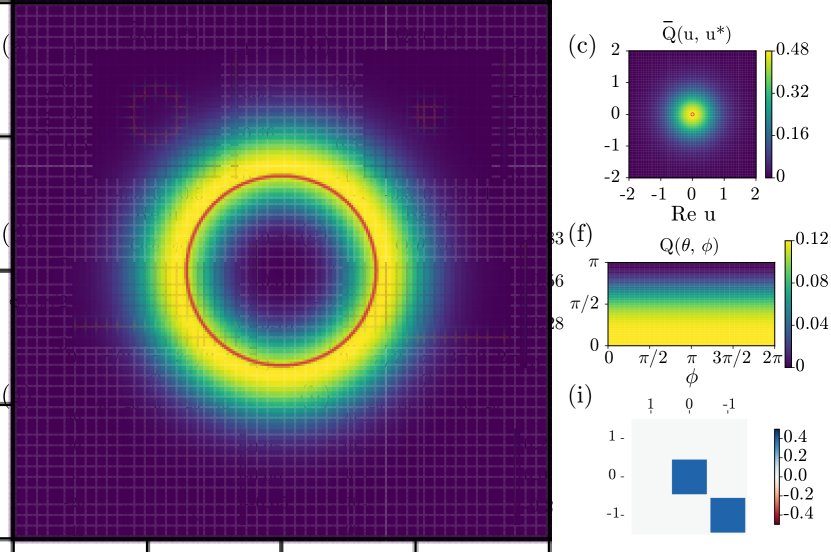
Figure 1: Limit-cycle oscillations of the quantum spin vdP oscillators with different spin numbers $J$. (a-c): $\bar{Q}(u,u^{*})$ functions on the complex plane with the corresponding classical limit cycles of Eq. (7) (red-thin lines). (d-f): $Q(\theta,\phi)$ functions on the unit sphere. (g-i): Elements of the steady-state density matrices $\rho_{ss}$. The spin numbers and other parameters are (a, d, g) $J=40$ and $(\omega,\gamma_{2})/\gamma_{1}=(-0.1,0.05)$, (b, e, h) $J=20$ and $(\omega,\gamma_{2})/\gamma_{1}=(-0.1,0.5)$, and (c, f, i) $J=1$ and $(\omega,\gamma_{2})/\gamma_{1}=(-0.1,100)$, where $\gamma_{1}=1$.

Stable limit-cycle oscillations in the phase space.- First, we illustrate the limit-cycle oscillations of the quantum spin vdP oscillator without external perturbations. Figure 1 shows the steady state $\rho_{ss}$ of Eq. (5) for three different values of the spin number $J$ and other parameter sets; Figs. 1(a)-1(c) depict the functions $\bar{Q}(u,u^{*})$ on the complex plane, Figs. 1(d)-1(f) depict the functions $Q(\theta,\phi)$ on the unit sphere, and Figs. 1(g)-1(i) show the elements of the steady-state density matrices $\rho_{ss}$. In Figs. 1(a)-1(c), we also show the stable limit-cycle solutions of Eq. (7) in the classical limit (see Supplemental Material).

We can observe that the function $\bar{Q}(u,u^{*})$ is localized around the classical limit cycle of Eq. (7) in all cases. Note that the quantum limit-cycle oscillation is more clearly observed in Fig. 1(a) with a high spin number $J$ and a small nonlinear damping parameter $\gamma_{2}$, where the system is in the semiclassical regime. The limit-cycle oscillation is also apparent in the $(\theta,\phi)$-representation as shown in Figs. 1(d)-1(f), where $Q(\theta,\phi)$ is localized around a certain value of $\theta$, while uniformly distributed without any preference for the phase $\phi$ Roulet and Bruder (2018a).

The steady-state density matrices in Figs. 1(g)-1(i) take non-zero values only on the diagonal elements, reflecting that the system has no preference for specific phase values. Additionally, the diagonal elements of each density matrix are concentrated around the elements $|{J,m}\rangle\langle{J,m}|$ with relatively small secondary spin quantum numbers $m$, and the element $|{J,J}\rangle\langle{J,J}|$ with the largest secondary spin quantum number, $m=J$, takes tiny values close to zero. This indicates that the system rarely reaches the highest spin state (See Supplemental Material for more details on the dependence on the spin number $J$).

Frequency entrainment to an external drive.- Next, we consider the frequency entrainment of a single quantum spin vdP oscillator to a periodic external drive. We introduce the external drive by adding the following Hamiltonian to the original Hamiltonian $H$ in Eq. (5):

$$H_{ex}=i\frac{E}{2}\left(e^{i\omega_{d}t}J^{\prime}_{-}-e^{-i\omega_{d}t}J^{\prime}_{+}\right),$$ (8)

where $E$ and $\omega_{d}$ represent the intensity and frequency of the external drive, respectively Roulet and Bruder (2018b). This external drive becomes equivalent to the harmonic drive for the quantum optical vdP oscillator in the high-spin limit Arecchi et al. (1972). In the rotating frame of the external drive frequency $\omega_{d}$, the master equation for the oscillator under the harmonic drive can be derived as Roulet and Bruder (2018a)

$$\dot{\rho} =-i[-\Delta J_{z}+EJ^{\prime}_{y},\rho]+\gamma_{1}\mathcal{D}[J^{\prime}_{+}]\rho+\gamma_{2}\mathcal{D}[(J^{\prime}_{-})^{2}]\rho,$$ (9)

where $\Delta=\omega_{d}-\omega$ represents the frequency detuning of the external drive from the oscillator and the rescaled operator $J^{\prime}_{y}=J_{y}/\sqrt{2J}$ with $J_{y}=-i(J_{+}-J_{-})/2$ was introduced.

To characterize the frequency entrainment, we use the observed frequency $\omega_{obs}$ defined as the peak frequency of the power spectrum $S(\omega)$ in the steady state,

$$\omega_{obs}=\mathop{\rm arg~{}max}\limits_{\omega}S(\omega),$$ (10)

$$S(\omega)=\int_{-\infty}^{\infty}d\tau e^{i\omega\tau}\left(\langle{J^{\prime}_{+}(\tau)J^{\prime}_{-}(0)}\rangle-\langle{J^{\prime}_{+}(\tau)}\rangle\langle{J^{\prime}_{-}(0)}\rangle\right),$$ (11)

where $\langle{A}\rangle={\rm Tr}\hskip 1.9919pt{[A\rho_{ss}]}$ represents the expectation value of $A$ with respect to the steady state $\rho_{ss}$ of Eq. (9) and $\langle{J^{\prime}_{+}(\tau)J^{\prime}_{-}(0)}\rangle$ is the correlation function of $J^{\prime}_{+}(\tau)$ and $J^{\prime}_{-}(0)$. We also introduce the following one-body order parameter to evaluate the phase coherence of the oscillator:

$$S_{1}={|S_{1}|}e^{i\phi_{1}}=\frac{\langle J^{\prime}_{-}\rangle}{\sqrt{\langle J_{z}+J\rangle}}.$$ (12)

The absolute value ${|S_{1}|}$ represents the degree of the phase coherence and $\phi_{1}$ characterizes the mean phase of the system. This quantity becomes equivalent to the order parameter $S^{a}_{1}=\frac{\langle a\rangle}{\sqrt{\langle a^{\dagger}a\rangle}}$ used for the quantum optical systems Lörch et al. (2016); Weiss et al. (2016) in the high-spin limit .

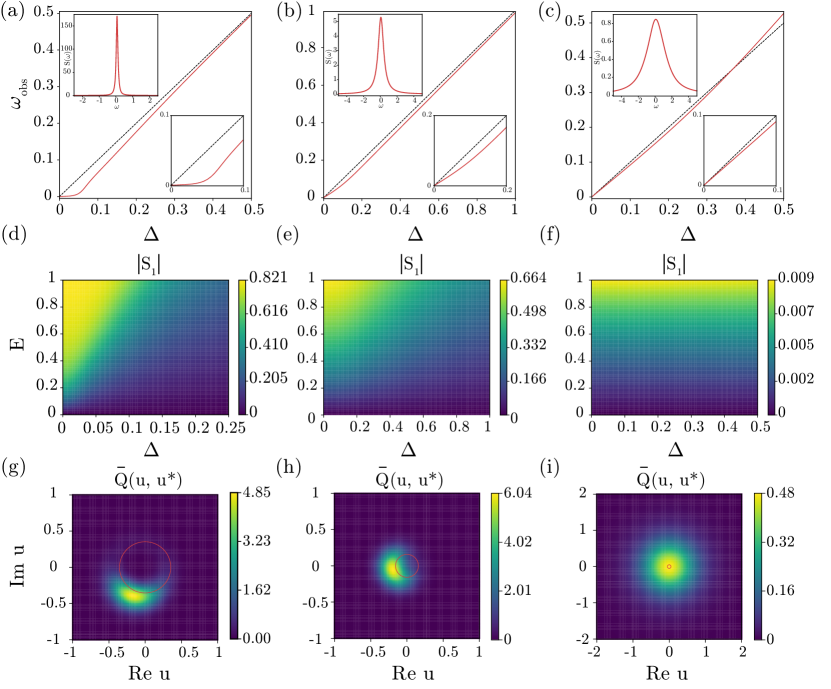
Figure 2: Frequency entrainment of a quantum spin vdP oscillator to a periodic external drive. (a-c): Observed frequencies $\omega_{obs}$. The inset at top left in each figure displays the power spectrum when $\Delta=0.1$. The inset at bottom right in each figure highlights the area with small detuning parameter $\Delta$. (d-f): Order parameters ${|S_{1}|}$ on the $\Delta-E$ plane, (g-i): $\bar{Q}(u,u^{*})$ functions on the complex plane with stable limit-cycle solutions of Eq. (7) (red-thin lines). The parameters are (a, d, g) $J=40$ and $\gamma_{2}/\gamma_{1}=0.05$, (b, e, h) $J=20$ and $\gamma_{2}/\gamma_{1}=0.5$, (c, f, i) $J=1$ and $\gamma_{2}/\gamma_{1}=100$, (a, b, c) $E/\gamma_{1}=1$, and (g, h, i) $(E,\Delta)/\gamma_{1}=(1,0.1)$, where $\gamma_{1}=1$.

Figure 2 shows the frequency entrainment of the quantum spin vdP oscillator for the same three parameter sets as in Figs. 1(a,d,g), 1(b,e,h), and 1(c,f,i); Figs. 2(a-c) plot the observed frequencies $\omega_{obs}$ with respect to the detuning parameter $\Delta$, Figs. 2(d-f) show the order parameters ${|S_{1}|}$ on the $\Delta$-$E$ parameter plane, and Figs. 2(g-i) show the $\bar{Q}$-distributions $\bar{Q}(u,u^{*})$ on the complex plane with the classical limit cycle of Eq. (7).

For the cases with large spin numbers, $J=40$ in Figs. 2(a,d,g) and $J=20$ in Figs. 2(b,e,h), we can clearly observe the frequency entrainment from the decrease in the observed frequency $\omega_{obs}$ in Figs. 2(a,b), Arnold tongues in Figs. 2(d,e), and the steady-state $\bar{Q}$ distributions localized around the phase-locking point in the classical limit in Figs. 2(g,h). The case with the larger spin number $J=40$ shows stronger tendency toward frequency entrainment than the case with $J=20$, as can be observed from the sharper decrease in the frequency difference between the oscillator and the external drive in Fig. 2(a) and narrower Arnold tongue in Fig. 2(d).

In contrast, the frequency entrainment is much weaker for the smallest spin-$1$ vdP oscillator ($J=1$); we cannot observe the Arnold tongue in Fig. 2(f) nor phase-locked $\bar{Q}$ distribution in Fig. 2(i) clearly due to the strong quantum noise. We can only see a small tendency to frequency entrainment from the slight decrease in the observed frequency $\omega_{obs}$ for small detuning parameter $\Delta$ in Fig. 2(c). However, $\omega_{obs}$ increases for larger $\Delta$, which never occurs in the quantum optical vdP oscillator. This is because, unlike the quantum optical vdP oscillator, the quantum spin vdP oscillator can reach the highest spin state by the energy pumping from the external drive, which has a particularly strong effect on the dynamics of the smallest spin-$1$ vdP oscillator.

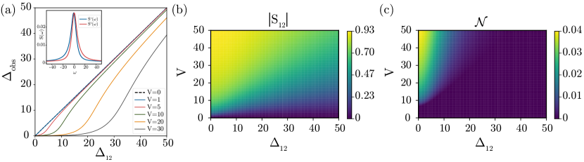
Figure 3: Frequency synchronization of two dissipatively coupled quantum spin vdP oscillators. The inset displays the power spectra with $\Delta_{12}=20,V=30$. (a): Dependence of the observed detuning $\Delta_{obs}$ on the parameter $\Delta_{12}$. (b, c): Dependence of (b) the order parameter ${|S_{12}|}$ and (c) the negativity $\mathcal{N}$ on the parameters $V$ and $\Delta_{12}$. The other parameters are $J=1$ and $\gamma_{2}/\gamma_{1}=100$. We set $\gamma_{1}=1$.

Frequency synchronization of two dissipatively coupled oscillators.- Next, we consider a pair of dissipatively coupled quantum spin vdP oscillators. The quantum master equation for the density matrix $\rho$ of this coupled system is generally given by

$$\dot{\rho}=\sum_{k=1,2}\left(-i[\omega_{k}J^{k}_{z},\rho]+\gamma_{1}\mathcal{D}[J^{\prime k}_{+}]\rho+\gamma_{2}\mathcal{D}[(J^{\prime k}_{-})^{2}]\rho\right)+V\mathcal{D}[J^{\prime 1}_{-}-J^{\prime 2}_{-}],$$ (13)

where $J^{k}_{z}$, $J^{\prime k}_{+}$, and $J^{\prime k}_{-}$ represent the (rescaled) angular momentum operators $J_{z},J^{\prime}_{+}$ and $J^{\prime}_{-}$ for the $k$-th oscillator $(k=1,2)$, $\omega_{k}$ represents the natural frequency of the $k$-th oscillator, and $V$ represents the strength of the dissipative coupling. We can show that, in the high-spin limit, this system becomes equivalent to a pair of dissipatively coupled quantum optical vdP oscillators Lee et al. (2014); Walter et al. (2015).

We define the observed frequency of each oscillator as the peak frequency of the power spectrum,

$$\omega^{k}_{obs}=\mathop{\rm arg~{}max}\limits_{\omega}S^{k}(\omega),\quad S^{k}(\omega)=\int_{-\infty}^{\infty}d\tau e^{i\omega\tau}\left(\langle{J^{\prime k}_{+}(\tau)J^{\prime k}_{-}(0)}\rangle-\langle{J^{\prime k}_{+}(\tau)}\rangle\langle{J^{\prime k}_{-}(0)}\rangle\right),$$ (14)

and use the observed detuning $\Delta_{obs}=\omega^{2}_{obs}-\omega^{1}_{obs}$ to evaluate the frequency synchronization of the two oscillators. We also introduce a two-body order parameter for evaluating the phase coherence between the two oscillators,

$$S_{12}={|S_{12}|}e^{i\phi_{12}}=\frac{\langle J^{\prime 1}_{+}J^{\prime 2}_{-}\rangle}{\sqrt{\langle J^{1}_{z}+J\rangle\langle J^{2}_{z}+J\rangle}},$$ (15)

which is, in the high-spin limit, equivalent to the quantum analog of the order parameter $S^{a}_{12}=\frac{\langle a_{1}^{{\dagger}}a_{2}\rangle}{\sqrt{\langle a_{1}^{\dagger}a_{1}\rangle}\sqrt{\langle a_{2}^{\dagger}a_{2}\rangle}}$ for quantum optical systems Weiss et al. (2016). Here, the absolute value ${|S_{12}|}$ represents the intensity of the phase coherence and $\phi_{12}$ characterizes the mean phase difference between the two oscillators.

To quantify the entanglement between the two oscillators, we use the negativity

$$\mathcal{N}=\frac{\left\|\rho^{\Gamma_{1}}\right\|_{1}-1}{2},$$ (16)

where $\rho^{\Gamma_{1}}$ represents the partial transpose of $\rho$ with respect to the subsystem of the oscillator $1$ and $\left\|X\right\|_{1}=\operatorname{Tr}|X|=\operatorname{Tr}\sqrt{X^{\dagger}X}$. The two oscillators are entangled when the negativity takes nonzero values Życzkowski et al. (1998); Vidal and Werner (2002).

Figure 3 shows the results for the two dissipatively coupled spin-$1$ vdP oscillators with the smallest possible spin number; Fig. 3(a) shows the dependence of $\Delta_{obs}$ on the frequency detuning $\Delta_{12}{=\omega_{2}-\omega_{1}}$, and Figs. 3(b) and 3(c) show the order parameter ${|S_{12}|}$ and negativity $\mathcal{N}$, respectively, with respect to the detuning $\Delta_{12}$ and coupling strength $V$. Here, we set $\omega_{1}=\Delta_{12}/2$ and $\omega_{2}=-\Delta_{12}/2$ in the numerical simulations. In Fig. 3(a), the frequency synchronization can be observed from the decrease in the observed detuning $\Delta_{obs}$, showing a stronger tendency toward frequency synchronization when the dissipative coupling strength $V$ is larger.

In remarkable contrast to the previous case for a single oscillator, we can clearly observe frequency synchronization, the Arnold tongue, and also the entanglement tongue Lee et al. (2014) between the two oscillators even for the smallest spin-$1$ case, similar to those observed for two dissipatively coupled quantum optical vdP oscillators Walter et al. (2015); Lee et al. (2014). This is because the dissipative coupling tends to bring the two systems to lower energy levels and prevents both systems from reaching the highest spin states, making the system dynamics unaffected by the finite dimensionality even in the case of the smallest spin-$1$ vdP oscillator. We also note that the above result is the first explicit observation of mutual frequency synchronization between a pair of single quantum spin-based limit-cycle oscillators, although macroscopic effects of quantum frequency synchronization between two networks of globally coupled quantum limit-cycle oscillators have been discussed in Nadolny and Bruder (2023).

Collective synchronization transition in a network of globally coupled oscillators- Finally, we analyze collective synchronization in a population of globally coupled quantum spin-$1$ vdP oscillators. We employ a mean-field approach similar to Nadolny and Bruder (2023) for globally coupled quantum spin-based oscillators.

We consider a large network of globally coupled $N$ quantum spin-$1$ vdP oscillators with identical properties. As in Lee et al. (2014) for the quantum optical system, we introduce an ansatz that the density matrix of the whole system can be described as a product of the subsystems as $\rho=\bigotimes_{n}\rho_{n}$ in the $N\to\infty$ limit, where $\rho_{n}$ represents the density matrix of the $n$-th oscillator. Because all oscillators are identical, the density matrix of the coupled system obeys an equation with a mean-field coupling (see Supplemental Material for the derivation),

$$\dot{\rho} =-i[\omega J_{z},\rho]+\gamma_{1}\mathcal{D}[J^{\prime}_{+}]\rho+\gamma_{2}\mathcal{D}[(J^{\prime}_{-})^{2}]\rho$$ (17)

$$+K\mathcal{D}[J^{\prime}_{-}]\rho+\frac{K}{2}\left(A^{*}[\rho,J^{\prime}_{-}]+A[J^{\prime}_{+},\rho]\right),$$ (18)

where $\omega$ determines the frequency and $K$ denotes the strength of the global coupling, and $A={\rm Tr}\hskip 1.9919pt[J^{\prime}_{-}\rho]$ and $A^{*}={\rm Tr}\hskip 1.9919pt[J^{\prime}_{+}\rho]$ represent the mean fields of $J^{\prime}_{+}$ and $J^{\prime}_{-}$, respectively.

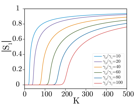
Figure 4 illustrates the dependence of the phase coherence ${|S_{1}|}$ on the coupling strength $K$ for several values of the nonlinear damping parameter $\gamma_{2}$. These values of $\gamma_{2}$ are sufficiently large that the finite dimensionality of the smallest spin-$1$ vdP oscillator does not significantly affect the system dynamics. We can clearly observe collective synchronization transitions from incoherent to coherent dynamics, i.e., sudden increase in $|S_{1}|$, around $K=20,40,75,110,145$, and $180$ for $\gamma_{2}/\gamma_{1}=10,20,40,60,80$, and $100$, respectively. The critical coupling strength $K$ at which the synchronization transition occurs increases with $\gamma_{2}$. Thus, the quantum analogue of the Kuramoto transition Kuramoto (1984) can also be observed clearly in globally coupled quantum spin-$1$ vdP oscillators.

Figure 4: Collective synchronization of globally coupled quantum spin vdP oscillators. Dependence of the phase coherence ${|S_{1}|}$ on the coupling strength $K$. The parameters are $J=1$ and $\omega=-20$. We set $\gamma_{1}=1$.

Possibility of experimental implementation.- We consider that the quantum spin vdP oscillator proposed in this study can be experimentally implemented with the currently available physical setups. Experimental realization of phase synchronization in spin-$1$ systems was recently reported in an ensemble of Rb atoms Laskar et al. (2020) and on the IBM Q system Koppenhöfer et al. (2020). Similarly, quantum synchronization of spin-$J$ systems would also be achievable in collective ensembles of qubits using such systems. The assumed dissipative negative damping and nonlinear damping could be experimentally engineered using the multi-level structures of atomic ensemble systems Poyatos et al. (1996); Lütkenhaus et al. (1998), as originally discussed in Roulet and Bruder (2018a). The ion trap system, considered as a candidate system for the potential realization of the quantum optical vdP oscillator Lee and Sadeghpour (2013), could also be used for experimental realization of the present quantum spin vdP oscillator.

Conclusion.- We proposed the quantum spin vdP oscillator as a prototypical model of limit-cycle oscillators in quantum spin systems. We demonstrated that it exhibits all representative features, i.e., stable limit-cycle oscillations, frequency entrainment, mutual synchronization, and collective synchronization, which are essentially important in the analysis of classical synchronization. We believe that the quantum spin vdP oscillator will provide valuable insights into novel features of quantum synchronization in many-body spin systems and future applications of quantum synchronization in the advancing fields of quantum technologies.

Acknowledgments.- Numerical simulations are performed by using QuTiP numerical toolbox Johansson et al. (2012, 2013). We acknowledge JSPS KAKENHI JP22K14274, JP22K11919, JP22H00516, and JST CREST JP-MJCR1913 for financial support.

I Overview of the spin coherent state

In this section, we give a more detailed overview of the spin coherent state introduced in the main text. Following Arecchi et al. Arecchi et al. (1972), we consider a spin-$J$ system consisting of an assembly of $N$ spin-$1/2$ atoms under a constant magnetic field in the $z$ direction and introduce the (collective) angular-momentum operators

$$J_{\mu}=\frac{1}{2}\sum_{n=1}^{N}\sigma_{\mu}^{n}\quad(\mu=x,y,z),\quad J_{\pm}=\sum_{n=1}^{N}\sigma_{\pm}^{n},\quad{\bm{J}}^{2}=J_{x}^{2}+J_{y}^{2}+J_{z}^{2},$$ (S1)

satisfying

$$\bm{J}^{2}|J,m\rangle=J(J+1)|J,m\rangle,\quad J_{\pm}\left|J,m\right\rangle=\sqrt{J(J+1)-m\left(m\pm 1\right)}\left|J,m\pm 1\right\rangle,$$ (S2)

$$J_{z}|J,m\rangle=m|J,m\rangle,\quad J_{x}=(J_{+}+J_{-})/2,~{}J_{y}=-i(J_{+}-J_{-})/2,$$ (S3)

where $\sigma_{\mu=x,y,z}^{n}$ are the Pauli matrices for the $n$th atom. This spin-$J$ system ($J=1/2,1,3/2,\ldots$) is described by a $(2J+1)$-dimensional subspace spanned by the degenerate eigenstates of ${\bm{J}}^{2}$ associated with the eigenvalue $J(J+1)$, i.e., $|{J,J}\rangle,|{J,J-1}\rangle,\cdots,|{J,-(J-1)}\rangle,|{J,-J}\rangle$.

The spin coherent state Radcliffe (1971); Arecchi et al. (1972), which is an analog of the standard coherent state in quantum optical systems Gardiner (1991); Carmichael (2007), is defined as

$$|{\theta,\phi}\rangle=R_{\theta,\phi}|{J,-J}\rangle,\quad R_{\theta,\phi}=e^{-i\theta(J_{x}\sin\phi-J_{y}\cos\phi)},$$ (S4)

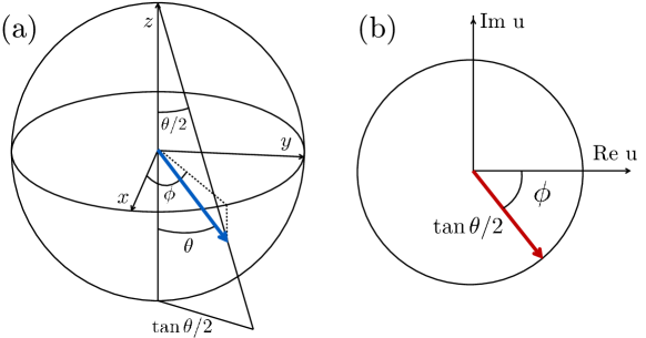
where the spin coherent state is specified by the point $(\theta,\phi)$ ($0\leq\theta<\pi$, $0\leq\phi\leq 2\pi$) on the unit sphere. The point $(\theta,\phi)$ on the unit sphere can be mapped to the point $(u,u^{*})$ on the complex plane as shown in Fig. S1 by introducing $u=\tan(\theta/2)e^{-i\phi}$, and the spin coherent state can be rewritten as

$$|{u}\rangle=|{\theta,\phi}\rangle=\sum_{m=-J}^{J}\binom{2J}{J+m}^{1/2}\frac{u^{m+J}}{(1+{|u|}^{2})^{J}}|{J,m}\rangle.$$ (S5)

The spin coherent states satisfy the following completeness relation:

$$\frac{(2J+1)}{4\pi}\int d\theta d\phi\sin\theta|{\theta,\phi}\rangle\langle{\theta,\phi}|=\frac{(2J+1)}{\pi}\int\frac{d^{2}u}{(1+{|u|}^{2})^{2}}|{u}\rangle\langle{u}|=\bm{1},$$ (S6)

where $\bm{1}$ is the $(2J+1)\times(2J+1)$ identity matrix.

We can also introduce the Hushimi $Q$ functions on the unit sphere Gilmore et al. (1975) and on the complex plane as

$$Q(\theta,\phi)=\frac{2J+1}{4\pi}\langle{\theta,\phi}|\rho|{\theta,\phi}\rangle,\quad Q(u,u^{*})=\frac{2J+1}{\pi}\langle{u}|\rho|{u}\rangle,$$ (S7)

respectively, which satisfy

$$\int d\theta d\phi\sin\theta Q(\theta,\phi)=\int d^{2}u\bar{Q}(u,u^{*})=1,\quad\bar{Q}(u,u^{*})=\frac{Q(u,u^{*})}{(1+{|u|}^{2})^{2}},$$ (S8)

where we introduced $\bar{Q}(u,u^{*})$ that includes the coefficient arising from the coordinate transformation.

Figure S1: Mapping of the point $|{\theta,\phi}\rangle$ on the unit sphere characterizing a spin coherent state to the point $(u,u^{*})$ on the complex plane.

II Semiclassical approximation and the classical limit

In this section, we derive Eq. (7) in the main text, which describes the deterministic dynamics in the classical limit of the quantum master equation (5). Defining $p=m+J$ and $|{p}\rangle=|{J,p-J}\rangle$ in Eq. (S5), we obtain

$$|{u}\rangle=\sum_{p=0}^{2J}\binom{2J}{p}^{1/2}\frac{u^{p}}{(1+{|u|}^{2})^{J}}|{p}\rangle,$$ (S9)

where

$$J_{+}\left|p\right\rangle=\sqrt{\left(2J-p\right)\left(p+1\right)}\left|p+1\right\rangle,$$ (S10)

$$J_{-}\left|p\right\rangle=\sqrt{\left(2J-p+1\right)p}\left|p-1\right\rangle,$$ (S11)

$$J_{z}|p\rangle=(p-J)|p\rangle.$$ (S12)

We define a projector $\Lambda$ to the spin coherent state and an weighted operator $\Lambda^{\prime}$ as

$$\Lambda=|{u}\rangle\langle{u}|=\sum_{p,q=0}^{2J}\Gamma_{p,q},\quad\Lambda^{\prime}=\sum_{p,q=0}^{2J}p\Gamma_{p,q},$$ (S13)

where

$$\Gamma_{p,q}=\binom{2J}{p}^{1/2}\binom{2J}{q}^{1/2}\frac{u^{p}(u^{*})^{q}}{(1+{|u|}^{2})^{2J}}|{p}\rangle\langle{q}|.$$ (S14)

With straightforward calculations, we obtain

$$J^{+}\Lambda=u^{-1}\Lambda^{\prime},\quad J^{-}\Lambda=u\left(2J\Lambda-\Lambda^{\prime}\right),\quad J^{z}\Lambda=\Lambda^{\prime}-J\Lambda,\quad\frac{\partial}{\partial u}\Lambda=\frac{-2u^{*}J}{1+{|u|}^{2}}\Lambda+u^{-1}\Lambda^{\prime},$$ (S15)

which lead to

$$J_{+}|{u}\rangle\langle{u}| =\left[\frac{\partial}{\partial u}+\frac{2u^{*}J}{1+{|u|}^{2}}\right]|{u}\rangle\langle{u}|,$$ (S16)

$$J_{-}|{u}\rangle\langle{u}| =\left[-u^{2}\frac{\partial}{\partial u}+\frac{2uJ}{1+{|u|}^{2}}\right]|{u}\rangle\langle{u}|,$$ (S17)

$$J_{z}|{u}\rangle\langle{u}| =\left[u\frac{\partial}{\partial u}+\frac{J({|u|}^{2}-1)}{1+{|u|}^{2}}\right]|{u}\rangle\langle{u}|.$$ (S18)

We introduce the $P$ quasiprobability functions Arecchi et al. (1972) on the unit sphere and on the complex plane as

$$\rho=\int d\theta d\phi\sin\theta P(\theta,\phi)|{\theta,\phi}\rangle\langle{\theta,\phi}|=\int d^{2}u\bar{P}(u,u^{*})|{u}\rangle\langle{u}|,\quad\bar{P}(u,u^{*})=4\frac{P(u,u^{*})}{(1+{|u|}^{2})^{2}},$$ (S19)

which satisfy

$$\int d\theta d\phi\sin\theta P(\theta,\phi)=\int d^{2}u\bar{P}(u,u^{*})=1.$$ (S20)

Here, we introduced the quasiprobability distribution function $\bar{P}(u,u^{*})$, which includes the coefficient arising from the coordinate transformation, in addition to $P(u,u^{*})$.

From Eq. (S16), we obtain the following correspondence between the actions of the angular-momentum operators on the density matrix $\rho$ and the actions of the differential operators on the quasiprobability distribution $\bar{P}(u,u^{*})$:

$$J_{+}\rho \leftrightarrow\left[-\frac{\partial}{\partial u}+\frac{2u^{*}J}{1+{|u|}^{2}}\right]\bar{P}(u,u^{*}),$$ (S21)

$$J_{-}\rho \leftrightarrow\left[\frac{\partial}{\partial u}u^{2}+\frac{2uJ}{1+{|u|}^{2}}\right]\bar{P}(u,u^{*}),$$ (S22)

$$J_{z}\rho \leftrightarrow\left[-\frac{\partial}{\partial u}u+\frac{J({|u|}^{2}-1)}{1+{|u|}^{2}}\right]\bar{P}(u,u^{*}).$$ (S23)

The above correspondence, expressing the actions of angular-momentum operators in the $P$ representation, was obtained in Narducci et al. (1975) for the function $P(\theta,\phi)$ in the $(\theta,\phi)$-coordinate representation.

Using Eq. (S21), the time evolution of the quasiprobability distribution $\bar{P}(u,u^{*})$ is obtained in the following form:

$$\frac{\partial\bar{P}(u,u^{*},t)}{\partial t} =\Big{[}-\sum_{j=1}^{2}\partial^{u}_{j}A_{j}(u,u^{*})+\frac{1}{2}\sum_{j=1}^{2}\sum_{k=1}^{2}\partial^{u}_{j}\partial^{u}_{k}D_{jk}(u,u^{*})+\cdots\Big{]}\bar{P}(u,u^{*},t),$$ (S24)

where $A_{j}(u,u^{*})$ represents the $j$th component ($j=1,2$) of a complex vector $\bm{A}(u,u^{*})=(A_{1}(u,u^{*}),A_{2}(u,u^{*}))\in\mathbb{C}^{2\times 1}$ with $A_{2}(u,u^{*})=A^{*}_{1}(u,u^{*})$, $D_{jk}(u,u^{*})$ represents the $(j,k)$-th component ($j,k=1,2$) of the symmetric diffusion matrix $\bm{D}(u,u^{*})\in\mathbb{C}^{2\times 2}$ with $D_{12}(u,u^{*})=D_{21}(u,u^{*})$, $\partial^{u}_{1}=\partial/\partial u$ and $\partial^{u}_{2}=\partial/\partial u^{*}$ are the complex partial derivatives with respect to the first and second arguments, i.e., $u$ and $u^{*}$, respectively, and $\left[\cdots\right]$ represents the complex partial derivative terms higher than the second order.

By explicitly calculating each term in Eq. (S24), the time evolution of $\bar{P}(u,u^{*},t)$ for the quantum spin vdP oscillator described by Eq. (5) in the main text is obtained as

$$\frac{\partial\bar{P}(u,u^{*},t)}{\partial t} =\left[-\sum_{j=1}^{2}\partial^{u}_{j}A_{j}(u,u^{*})+\frac{1}{2}\sum_{j=1}^{2}\sum_{k=1}^{2}\partial^{u}_{j}\partial^{u}_{k}D_{jk}(u,u^{*})\right.$$ (S25)

$$-\frac{\gamma_{2}}{(2J)^{2}}\left(\frac{\partial^{3}}{\partial u^{2}\partial u^{*}}\frac{2u{|u|}^{6}}{1+{|u|}^{2}}({|u|}^{2}-2J+1)\right.$$ (S26)

$$\left.-\frac{\partial^{3}}{\partial u^{3}}\frac{u^{3}}{1+{|u|}^{2}}((2J+1){|u|}^{2}-2J+1)+H.c.\right)$$ (S27)

$$\left.+\frac{\gamma_{2}}{(2J)^{2}}\frac{1}{2}\left(-\frac{\partial^{4}}{\partial u^{4}}u^{4}+\frac{\partial^{4}}{\partial u^{2}\partial u^{*2}}{|u|}^{8}+H.c.\right)\right]\bar{P}(u,u^{*},t),$$ (S28)

where

$$\bm{A}(u,u^{*}) =\left(\begin{matrix}\left(\frac{\gamma_{1}}{2J}(J+1)-i\omega\right)u-\frac{\gamma_{2}}{(2J)^{2}}\frac{1}{(1+{|u|}^{2})^{3}}2J(2J-1)u{|u|}^{2}({|u|}^{4}+(2J+1){|u|}^{2}+2J)\\ \left(\frac{\gamma_{1}}{2J}(J+1)+i\omega\right)u^{*}-\frac{\gamma_{2}}{(2J)^{2}}\frac{1}{(1+{|u|}^{2})^{3}}2J(2J-1)u^{*}{|u|}^{2}({|u|}^{4}+(2J+1){|u|}^{2}+2J)\\ \end{matrix}\right)$$ (S29)

and

$$\bm{D}(u,u^{*})=\scalebox{0.8}{$\displaystyle\left(\begin{matrix}\frac{\gamma_{1}}{2J}u^{2}+\frac{\gamma_{2}}{(2J)^{2}}\frac{1}{(1+{|u|}^{2})^{2}}2J(2J-1)u^{2}({|u|}^{4}+4{|u|}^{2}-1)&\frac{\gamma_{1}}{2J}+\frac{\gamma_{2}}{(2J)^{2}}\frac{4{|u|}^{6}}{(1+{|u|}^{2})^{2}}({|u|}^{4}+2(-J+1){|u|}^{2}+(-2J+1)^{2})\\ \frac{\gamma_{1}}{2J}+\frac{\gamma_{2}}{(2J)^{2}}\frac{4{|u|}^{6}}{(1+{|u|}^{2})^{2}}({|u|}^{4}+2(-J+1){|u|}^{2}+(-2J+1)^{2})&\frac{\gamma_{1}}{2J}u^{*2}+\frac{\gamma_{2}}{(2J)^{2}}\frac{1}{(1+{|u|}^{2})^{2}}2J(2J-1)u^{*2}({|u|}^{4}+4{|u|}^{2}-1)\\ \end{matrix}\right)$}.$$ (S30)

Rescaling the complex variable as $u=\frac{u^{\prime}}{\sqrt{2J}}$, we obtain the evolution equation for the quasiprobability distribution in the $\bar{P}$ representation of the rescaled complex variables $u^{\prime}$ and $u^{\prime*}$ as

$$\frac{\partial\bar{P}(u^{\prime},u^{\prime*},t)}{\partial t} =\left[-\sum_{j=1}^{2}\partial^{u^{\prime}}_{j}A_{j}(u^{\prime},u^{\prime*})+\frac{1}{2}\sum_{j=1}^{2}\sum_{k=1}^{2}\partial^{u^{\prime}}_{j}\partial^{u^{\prime}}_{k}D_{jk}(u^{\prime},u^{\prime*})\right.$$ (S31)

$$-\frac{\gamma_{2}}{(2J)^{2}}\left(\frac{\partial^{3}}{\partial u^{\prime 2}\partial u^{\prime*}}\frac{2u^{\prime}\frac{{|u^{\prime}|}^{6}}{(2J)^{2}}}{(1+\frac{{|u^{\prime}|}^{2}}{2J})}(\frac{{|u^{\prime}|}^{2}}{2J}-2J+1)\right.$$ (S32)

$$-\left.\frac{\partial^{3}}{\partial u^{\prime 3}}\frac{u^{\prime 3}}{1+\frac{{|u^{\prime}|}^{2}}{2J}}((2J+1)\frac{{|u^{\prime}|}^{2}}{2J}-2J+1)+H.c.\right)$$ (S33)

$$\left.+\frac{\gamma_{2}}{(2J)^{2}}\frac{1}{2}\left(-\frac{\partial^{4}}{\partial u^{\prime 4}}u^{\prime 4}+\frac{\partial^{4}}{\partial u^{\prime 2}\partial u^{\prime*2}}\frac{{|u^{\prime}|}^{8}}{(2J)^{2}}+H.c.\right)\right]\bar{P}(u^{\prime},u^{\prime*},t)$$ (S34)

with

$$\bm{A}(u^{\prime},u^{\prime*}) =\left(\begin{matrix}\left(\frac{\gamma_{1}}{2J}(J+1)-i\omega\right)u^{\prime}-\frac{\gamma_{2}}{(2J)^{2}}\frac{1}{(1+\frac{{|u^{\prime}|}^{2}}{2J})^{3}}(2J-1)u^{\prime}{|u^{\prime}|}^{2}(\frac{{|u^{\prime}|}^{4}}{(2J)^{2}}+(2J+1)\frac{{|u^{\prime}|}^{2}}{2J}+2J)\\ \left(\frac{\gamma_{1}}{2J}(J+1)+i\omega\right)u^{\prime*}-\frac{\gamma_{2}}{(2J)^{2}}\frac{1}{(1+\frac{{|u^{\prime}|}^{2}}{2J})^{3}}(2J-1)u^{\prime*}{|u^{\prime}|}^{2}(\frac{{|u^{\prime}|}^{4}}{(2J)^{2}}+(2J+1)\frac{{|u^{\prime}|}^{2}}{2J}+2J)\\ \end{matrix}\right)$$ (S35)

and

$$\bm{D}(u^{\prime},u^{\prime*})=\scalebox{0.8}{$\displaystyle\left(\begin{matrix}\frac{\gamma_{1}}{2J}u^{\prime 2}+\frac{\gamma_{2}}{(2J)^{2}}\frac{1}{(1+\frac{{|u^{\prime}|}^{2}}{2J})^{2}}2J(2J-1)u^{\prime 2}(\frac{{|u^{\prime}|}^{4}}{(2J)^{2}}+4\frac{{|u^{\prime}|}^{2}}{2J}-1)&\gamma_{1}+\frac{\gamma_{2}}{(2J)^{2}}\frac{4\frac{{|u^{\prime}|}^{6}}{(2J)^{2}}}{(1+\frac{{|u^{\prime}|}^{2}}{2J})^{2}}(\frac{{|u^{\prime}|}^{4}}{(2J)^{2}}+2(-J+1)\frac{{|u^{\prime}|}^{2}}{2J}+(-2J+1)^{2})\\ \gamma_{1}+\frac{\gamma_{2}}{(2J)^{2}}\frac{4\frac{{|u^{\prime}|}^{6}}{(2J)^{2}}}{(1+\frac{{|u^{\prime}|}^{2}}{2J})^{2}}(\frac{{|u^{\prime}|}^{4}}{(2J)^{2}}+2(-J+1)\frac{{|u^{\prime}|}^{2}}{2J}+(-2J+1)^{2})&\frac{\gamma_{1}}{2J}u^{\prime*2}+\frac{\gamma_{2}}{(2J)^{2}}\frac{1}{(1+\frac{{|u^{\prime}|}^{2}}{2J})^{2}}2J(2J-1)u^{\prime*2}(\frac{{|u^{\prime}|}^{4}}{(2J)^{2}}+4\frac{{|u^{\prime}|}^{2}}{2J}-1)\\ \end{matrix}\right)$},$$ (S36)

where the complex partial derivatives with respect to $u^{\prime}$ and $u^{\prime*}$ are defined as $\partial^{u^{\prime}}_{1}=\partial/\partial u^{\prime}$ and $\partial^{u^{\prime}}_{2}=\partial/\partial u^{\prime*}$, respectively.

Assuming that the spin number $J$ is sufficiently large and neglecting the terms of order $\mathcal{O}(1/J)$ in Eq. (S31), we obtain the approximate semiclassical FPE representing the time evolution of the $\bar{P}$ function as

$$\frac{\partial\bar{P}(u^{\prime},u^{\prime*},t)}{\partial t} =\left[-\sum_{j=1}^{2}\partial^{u^{\prime}}_{j}A_{j}(u^{\prime},u^{\prime*})+\frac{1}{2}\sum_{j=1}^{2}\sum_{k=1}^{2}\partial^{u^{\prime}}_{j}\partial^{u^{\prime}}_{k}D_{jk}(u^{\prime},u^{\prime*})\right]\bar{P}(u^{\prime},u^{\prime*},t)$$ (S37)

with

$$\bm{A}(u^{\prime},u^{\prime*}) =\left(\begin{matrix}\left(\frac{\gamma_{1}}{2}-i\omega\right)u^{\prime}-\gamma_{2}u^{\prime}{|u^{\prime}|}^{2}\\ \left(\frac{\gamma_{1}}{2}+i\omega\right)u^{\prime*}-\gamma_{2}u^{\prime*}{|u^{\prime}|}^{2}\\ \end{matrix}\right)$$ (S38)

and

$$\bm{D}(u^{\prime},u^{\prime*})=\scalebox{0.8}{$\displaystyle\left(\begin{matrix}-\gamma_{2}u^{\prime 2}&\gamma_{1}\\ \gamma_{1}&-\gamma_{2}u^{\prime*2}\\ \end{matrix}\right)$},$$ (S39)

which has the same form as the semiclassical FPE for the quantum optical vdP oscillator obtained in Kato et al. (2019).

Now, further assuming $\gamma_{2}\ll\gamma_{1}$ and neglecting the effect of quantum noise, we obtain the deterministic dynamics in the classical limit as

$$\dot{u^{\prime}}=\left(\frac{\gamma_{1}}{2}-i\omega\right)u^{\prime}-\gamma_{2}u^{\prime}{|u^{\prime}|}^{2},$$ (S40)

which is equivalent to the deterministic dynamics in the classical limit of the quantum optical vdP oscillator in Eq. (S43) described in the next section. Using the original complex variable $u^{\prime}=\sqrt{2J}u$, we obtain

$$\dot{u}=\left(\frac{\gamma_{1}}{2}-i\omega\right)u-2J\gamma_{2}u{|u|}^{2},$$ (S41)

which gives the deterministic dynamics, Eq. (7), in the main text.

We note that, although the limit-cycle solution in the classical limit is derived via the $\bar{P}$ function, which is similar to but slightly different from the $\bar{Q}$ function, the function $\bar{Q}(u,u^{*})$ localizes near the stable limit-cycle solution in the classical limit as shown in the figures in the main text. Note also that the phase-space representation is singular at the point $\theta=\pi$ (i.e., the north pole where $\phi$ is undefined) on the sphere in Eq. (S4), and we excluded this point in the above derivation Arecchi et al. (1972).

We also note that in Ref. Dutta et al. (2024), a different semiclassical approach has been employed to introduce limit-cycle oscillations in the classical limit of quantum spin systems.

III Correspondence to the quantum optical vdP oscillator in the high-spin limit

In this section, we show that the quantum spin vdP oscillator becomes equivalent to the quantum optical vdP oscillator in the high-spin limit ($J\to\infty$). In this limit, through the process known as the group contraction Inonu and Wigner (1953); Segal et al. (1951), the operators for the spin systems can be related to those for the quantum optical systems as Arecchi et al. (1972)

$$u\leftrightarrow\alpha/\sqrt{2J},\quad J_{-}\leftrightarrow\sqrt{2J}a,\quad J_{+}\leftrightarrow\sqrt{2J}a^{\dagger},\quad J_{z}\leftrightarrow a^{\dagger}a-J,$$ (S42)

where $a$ and $a^{\dagger}$ represent the annihilation and creation operators for the harmonic oscillator, respectively. By this correspondence, the spin coherent state in the high-spin limit becomes equivalent to the quantum optical coherent state in the harmonic-oscillator systems Carmichael (2007); Gardiner (1991). Note that, though not used in this paper, we can also consider the correspondence in the high-spin limit of the Holstein-Primakoff transformation Holstein and Primakoff (1940), in which the lowering operator corresponds to the creation operator.

Using Eq. (S42), the quantum master equation (5) in the main text can be transformed to

$$\dot{\rho}=-i\left[\omega a^{{\dagger}}a,\rho\right]+\gamma_{1}\mathcal{D}[a^{{\dagger}}]\rho+\gamma_{2}\mathcal{D}[a^{2}]\rho$$ (S43)

in the high-spin limit, which is the quantum master equation of a quantum optical vdP oscillator Lee and Sadeghpour (2013). The time evolution of $\bar{P}(u,u^{*},t)$ in Eq. (S25) can also be transformed to the time evolution of the $P$ distribution $\bar{P}(\alpha,\alpha^{*},t)$ in the quantum optical coherent-state representation,

$$\frac{\partial P(\alpha,\alpha^{*},t)}{\partial t}=\Big{[}-\sum_{j=1}^{2}\partial^{\alpha}_{j}\{A_{j}(\alpha,\alpha^{*}),t)\}+\frac{1}{2}\sum_{j=1}^{2}\sum_{k=1}^{2}\partial^{\alpha}_{j}\partial^{\alpha}_{k}\{D_{jk}(\alpha,\alpha^{*})\}\Big{]}P(\alpha,\alpha^{*},t)$$ (S44)

with

$$\bm{A}(\alpha,\alpha^{*})=\left(\begin{matrix}\left(\frac{\gamma_{1}}{2}-i\omega\right)\alpha-\gamma_{2}\alpha{|\alpha|}^{2}\\ \left(\frac{\gamma_{1}}{2}+i\omega\right)\alpha^{*}-\gamma_{2}\alpha^{*}{|\alpha|}^{2}\\ \end{matrix}\right)$$ (S45)

and

$$\bm{D}(\alpha,\alpha^{*})=\left(\begin{matrix}-\gamma_{2}\alpha^{2}&\gamma_{1}\\ \gamma_{1}&-\gamma_{2}\alpha^{*2}\\ \end{matrix}\right),$$ (S46)

where the complex partial derivatives are defined as $\partial^{\alpha}_{1}=\partial/\partial\alpha$ and $\partial^{\alpha}_{2}=\partial/\partial\alpha^{*}$. This FPE is equivalent to the FPE for a quantum optical vdP oscillator Kato et al. (2019).

The deterministic dynamics in the classical limit, i.e., the dynamics described by the drift vector field in Eq. (S44), is given by

$$\dot{\alpha}=\left(\frac{\gamma_{1}}{2}-i\omega\right)\alpha-\gamma_{2}\alpha^{*}\alpha^{2},$$ (S47)

which is equivalent to the deterministic equation obtained in the classical limit of the quantum optical vdP oscillator described by Eq. (S43) Lee and Sadeghpour (2013); Walter et al. (2014); Lee et al. (2014). This equation represents the normal form of the supercritical Hopf bifurcation, which can be derived from the classical vdP oscillator with a weak nonlinearity Van Der Pol (1927) near the Hopf bifurcation point.

Finally, we note that the nonlinear oscillator in Eq. (S47) is known as the Stuart-Landau oscillator Kuramoto (1984) in the literature, and the quantum optical vdP oscillator in Eq. (S43) has also been referred to as the quantum Stuart-Landau oscillator recently Chia et al. (2020); Mok et al. (2020); C. W. Wachtler and Munro (2020). Therefore, the quantum spin vdP oscillator proposed in this study may also be called the quantum spin Stuart-Landau oscillator.

IV Derivation of the mean-field equation for globally coupled oscillators

In this appendix, we derive the mean-field equation (17) in the main text. Our starting point is the following quantum master equation for the network of globally coupled $N$ quantum spin vdP oscillators:

$$\dot{\rho} =\sum_{k=1}^{N}\left(-i[\omega J^{k}_{z},\rho]+\gamma_{1}\mathcal{D}[J^{\prime k}_{+}]\rho+\gamma_{2}\mathcal{D}[(J^{\prime k}_{-})^{2}]\rho\right)$$ (S48)

$$+\frac{K}{N}\sum_{k=1}^{N}\sum_{k^{\prime}=1,k^{\prime}<k}^{N}\mathcal{D}[(J^{\prime k^{\prime}}_{-}-J^{\prime k}_{-})]\rho,$$ (S49)

where $J^{k}_{z}$, $J^{\prime k}_{+}$, and $J^{\prime k}_{-}$ represent the (rescaled) angular momentum operators for the $k$-th$~{}(k=1,2,\ldots,N)$ oscillator, $\omega_{k}$ represents the natural frequency of the $k$-th oscillator, and $K$ represents the strength of the dissipative coupling. Note that $\mathcal{D}[L]=\mathcal{D}[-L]$ for a given operator $L$.

We introduce the ansatz that the density matrix of the whole system is described as the product of the density matrices of the subsystems $\rho=\bigotimes_{n}\rho_{n}$. Then, by taking the partial trace over all $\rho_{k}^{\prime}$ other than $\rho_{k}$ ($k^{\prime}\neq k$), the time evolution of the $k$-th subsystem $\rho_{k}$ is described as

$$\dot{\rho}_{k} =\left(-i[\omega J^{k}_{z},\rho_{k}]+\gamma_{1}\mathcal{D}[J^{\prime k}_{+}]\rho_{k}+\gamma_{2}\mathcal{D}[(J^{\prime k}_{-})^{2}]\rho_{k}\right)$$ (S50)

$$+\frac{K(N-1)}{N}\mathcal{D}[J^{\prime k}_{-}]\rho_{k}+\frac{K}{2}\left(A_{N}^{*}[\rho_{k},J^{\prime k}_{-}]+A_{N}[J^{\prime k}_{+},\rho_{k}]\right),$$ (S51)

where

$$A_{N}=\frac{1}{N}\sum_{k^{\prime}=1,k^{\prime}\neq k}^{N}{\rm Tr}\hskip 1.9919pt[J^{\prime k}_{-}\rho_{k}],\quad A^{*}_{N}=\frac{1}{N}\sum_{k^{\prime}=1,k^{\prime}\neq k}^{N}{\rm Tr}\hskip 1.9919pt[J^{\prime k}_{+}\rho_{k}],$$ (S52)

are the averages of the expectation values of $J^{\prime k}_{+}$ and $J^{\prime k}_{-}$ taken over all oscillators.

In the limit $N\to\infty$ Spohn (1980), we obtain the mean-field equation in the form

$$\dot{\rho} =-i[\omega J_{z},\rho]+\gamma_{1}\mathcal{D}[J^{\prime}_{+}]\rho+\gamma_{2}\mathcal{D}[(J^{\prime}_{-})^{2}]\rho$$ (S53)

$$+K\mathcal{D}[J^{\prime}_{-}]\rho+\frac{K}{2}\left(A^{*}[\rho,J^{\prime}_{-}]+A[J^{\prime}_{+},\rho]\right),$$ (S54)

where $A={\rm Tr}\hskip 1.9919pt[J^{\prime}_{-}\rho]$ and $A^{*}={\rm Tr}\hskip 1.9919pt[J^{\prime}_{+}\rho]$, and the oscillator index $k$ was dropped because all oscillators are statistically equivalent.

V Dependence of purity on the spin number

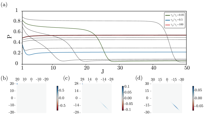
In this section, to investigate the dependence of the system dynamics on the spin number $J$, we examine the purity $P={\rm Tr}\hskip 1.9919pt[\rho_{ss}^{2}]$ in the steady state, which characterizes qualitative changes in the properties of the density matrix $\rho$.

Figure S2(a) plots the purity $P$ as a function of the spin number $J$ for various values of the nonlinear damping parameter $\gamma_{2}$. When the nonlinear damping parameter $\gamma_{2}$ is relatively small, the purity $P$ undergoes a transition from a large value to a small value as $J$ increases. For example, such transitions are observed in Fig. S2(a) around $J=J_{0}=28$ and $J_{0}=2$ for the cases with $\gamma_{2}/\gamma_{1}=0.05$ and $0.5$, respectively. For a large nonlinear damping parameter $\gamma_{2}$, such as $\gamma_{2}/\gamma_{1}=100$, such a transition cannot be observed. We also illustrate density matrices near the transition points in Figs. S2(b-d) for $\gamma_{2}/\gamma_{1}=0.05$, where the values of $J$ are (b) $J=20$, (c) $J=28$, and (d) $J=30$, respectively.

The reason for the transitions in the purity $P$ are as follows. Before the transitions, the effect of negative damping is relatively stronger than the effect of nonlinear damping, i.e. the energy pumping is relatively stronger than the energy dissipation, causing the diagonal elements of the density matrix to concentrate on the state $|{J,J}\rangle\langle{J,J}|$. After the transitions, the effect of negative damping is relatively weaker than the effect of nonlinear damping, i.e. the energy pumping is relatively weaker than the energy dissipation, causing the diagonal elements of the density matrix to concentrate on the states $|{J,m}\rangle\langle{J,m}|$ with relatively small spin numbers $m$.

In Figs. 1(a)-(i) in the main text, we can observe the limit-cycle oscillation when the system’s spin number $J$ is larger than the spin number $J_{0}$ at which the purity $P$ shows a transition in Fig. S2(a), whereas the limit-cycle oscillation cannot be observed clearly when the system’s spin number $J$ is smaller than $J_{0}$. Thus, the spin number $J_{0}$ characterizes whether clear limit-cycle oscillations can be observed or not in the quantum spin vdP oscillator.

Figure S2: (a): Dependence of the purity $P$ on the spin number $J$. $\gamma_{2}/\gamma_{1}=0.05$ (green-thin line), $\gamma_{2}/\gamma_{1}=0.5$ (blue-thin line), $\gamma_{2}/\gamma_{1}=100$ (red-thin line), and $\gamma_{2}/\gamma_{1}=(0.03,0.07,0.1,1,5,10,50,500)$ (black-dotted lines). (b-d): Elements of the density matrices $\rho_{ss}$ for the parameters $(\omega,\gamma_{2})/\gamma_{1}=(-0.1,0.05)$ with (b) $J=20$, (c) $J=28$, and (d) $J=30$. We set $\gamma_{1}=1$.

References

Winfree (2001)A. T. Winfree, The geometry of
biological time (Springer, New York, 2001).
Kuramoto (1984)Y. Kuramoto, Chemical oscillations,
waves, and turbulence (Springer, Berlin, 1984).
Ermentrout and Terman (2010)G. B. Ermentrout and D. H. Terman, Mathematical foundations
of neuroscience (Springer, New York, 2010).
Pikovsky et al. (2001)A. Pikovsky, M. Rosenblum,
and J. Kurths, Synchronization: a universal concept
in nonlinear sciences (Cambridge University
Press, Cambridge, 2001).
Glass and Mackey (1988)L. Glass and M. C. Mackey, From clocks to chaos:
the rhythms of life (Princeton University Press, Princeton, 1988).
Strogatz (1994)S. Strogatz, Nonlinear dynamics and
chaos (Westview Press, 1994).
Laskar et al. (2020)A. W. Laskar, P. Adhikary,
S. Mondal, P. Katiyar, S. Vinjanampathy, and S. Ghosh, Physical Review Letters 125, 013601 (2020).
Krithika et al. (2022)V. Krithika, P. Solanki,
S. Vinjanampathy, and T. Mahesh, Physical Review A 105, 062206 (2022).
Koppenhöfer et al. (2020)M. Koppenhöfer, C. Bruder, and A. Roulet, Physical Review Research 2, 023026 (2020).
Lee and Sadeghpour (2013)T. E. Lee and H. Sadeghpour, Physical Review Letters 111, 234101 (2013).
Walter et al. (2014)S. Walter, A. Nunnenkamp,
and C. Bruder, Physical
Review Letters 112, 094102 (2014).
Sonar et al. (2018)S. Sonar, M. Hajdušek, M. Mukherjee, R. Fazio,
V. Vedral, S. Vinjanampathy, and L.-C. Kwek, Physical Review Letters 120, 163601 (2018).
Lörch et al. (2016)N. Lörch, E. Amitai,
A. Nunnenkamp, and C. Bruder, Physical Review Letters 117, 073601 (2016).
Lee et al. (2014)T. E. Lee, C.-K. Chan, and S. Wang, Physical Review E 89, 022913 (2014).
Walter et al. (2015)S. Walter, A. Nunnenkamp,
and C. Bruder, Annalen der
Physik 527, 131
(2015).
Es’ haqi Sani et al. (2020)N. Es’ haqi Sani, G. Manzano, R. Zambrini, and R. Fazio, Physical Review
Research 2, 023101
(2020).
Bastidas et al. (2015)V. Bastidas, I. Omelchenko, A. Zakharova, E. Schöll, and T. Brandes, Physical Review E 92, 062924 (2015).
Kato et al. (2019)Y. Kato, N. Yamamoto, and H. Nakao, Physical Review
Research 1, 033012
(2019).
Mok et al. (2020)W.-K. Mok, L.-C. Kwek, and H. Heimonen, Physical Review
Research 2, 033422
Roulet and Bruder (2018a)A. Roulet and C. Bruder, Physical Review Letters 121, 053601 (2018a).
Roulet and Bruder (2018b)A. Roulet and C. Bruder, Physical Review Letters 121, 063601 (2018b).
Koppenhöfer and Roulet (2019)M. Koppenhöfer and A. Roulet, Physical Review A 99, 043804 (2019).
Xu et al. (2014)M. Xu, D. A. Tieri,
E. Fine, J. K. Thompson, and M. J. Holland, Physical Review Letters 113, 154101 (2014).
Xu and Holland (2015)M. Xu and M. Holland, Physical
Review Letters 114, 103601 (2015).
Kato and Nakao (2022)Y. Kato and H. Nakao, Chaos: An
Interdisciplinary Journal of Nonlinear Science 32, 063133 (2022).
Kato and Nakao (2023)Y. Kato and H. Nakao, New Journal of
Physics 25, 023012
(2023).
Solanki et al. (2023)P. Solanki, F. M. Mehdi,
M. Hajdušek, and S. Vinjanampathy, Physical Review
A 108, 022216 (2023).
Solanki et al. (2022)P. Solanki, N. Jaseem,
A 105, L020401 (2022).
Chia et al. (2020)A. Chia, L. Kwek, and C. Noh, Physical Review E 102, 042213 (2020).
Arosh et al. (2021)L. B. Arosh, M. Cross, and R. Lifshitz, Physical Review Research 3, 013130 (2021).
Galve et al. (2017)F. Galve, G. L. Giorgi, and R. Zambrini, in Lectures on General Quantum
Correlations and their Applications (Springer, 2017) pp. 393–420.
Buča et al. (2022)B. Buča, C. Booker,
and D. Jaksch, SciPost Physics 12, 097 (2022).
Schmolke and Lutz (2022)F. Schmolke and E. Lutz, Physical
Review Letters 129, 250601 (2022).
Tan et al. (2022)R. Tan, C. Bruder, and M. Koppenhöfer, Quantum 6, 885 (2022).
Eneriz et al. (2019)H. Eneriz, D. Rossatto,
F. A. Cárdenas-López, E. Solano, and M. Sanz, Scientific Reports 9, 1 (2019).
Jaseem et al. (2020)N. Jaseem, M. Hajdušek, P. Solanki, L.-C. Kwek,
R. Fazio, and S. Vinjanampathy, Physical Review Research 2, 043287 (2020).
Tindall et al. (2020)J. Tindall, C. S. Munoz,
B. Buča, and D. Jaksch, New Journal of Physics 22, 013026 (2020).
Cabot et al. (2019)A. Cabot, G. L. Giorgi,
F. Galve, and R. Zambrini, Physical Review Letters 123, 023604 (2019).
Cabot et al. (2021)A. Cabot, G. L. Giorgi, and R. Zambrini, New Journal of
Physics 23, 103017
(2021).
Nadolny and Bruder (2023)T. Nadolny and C. Bruder, Physical Review Letters 131, 190402 (2023).
Van Der Pol (1927)B. Van
Der Pol, The
London, Edinburgh, and Dublin Philosophical Magazine and Journal of Science 3, 65 (1927).
Van Der Pol and Van
Der Mark (1928)B. Van
Der Pol and J. Van
Der Mark, The
London, Edinburgh, and Dublin Philosophical Magazine and Journal of Science 6, 763 (1928).
Nagumo et al. (1962)J. Nagumo, S. Arimoto, and S. Yoshizawa, Proceedings of the
IRE 50, 2061 (1962).
Note (1)The quantum optical vdP oscillator has also been referred to
as the quantum Stuart-Landau oscillator recently because the system in the
classical limit is the classical Stuart-Landau oscillator, which is a normal
form of the supercritical Hopf bifurcation and slightly different from the
classical vdP oscillator. See Supplemental Material at [URL will be inserted
by the publisher] for a detailed discussion.
Zhirov and Shepelyansky (2008)O. Zhirov and D. Shepelyansky, Physical Review Letters 100, 014101 (2008).
Parra-López and Bergli (2020)Á. Parra-López and J. Bergli, Physical Review A 101, 062104 (2020).
Radcliffe (1971)J. Radcliffe, Journal of Physics A: General Physics 4, 313 (1971).
Arecchi et al. (1972)F. Arecchi, E. Courtens,
R. Gilmore, and H. Thomas, Physical Review A 6, 2211 (1972).
Gardiner (1991)C. W. Gardiner, Quantum Noise (Springer, New York, 1991).
Carmichael (2007)H. J. Carmichael, Statistical Methods
in Quantum Optics 1, 2 (Springer, New York, 2007).
Gilmore et al. (1975)R. Gilmore, C. Bowden, and L. Narducci, Physical Review
A 12, 1019 (1975).
Weiss et al. (2016)T. Weiss, A. Kronwald, and F. Marquardt, New Journal of
Physics 18, 013043
(2016).
Note (2)If , we obtain , and denoting ,
it converge to in the high-spin limit.
Życzkowski et al. (1998)K. Życzkowski, P. Horodecki, A. Sanpera,
and M. Lewenstein, Physical Review
A 58, 883 (1998).
Vidal and Werner (2002)G. Vidal and R. F. Werner, Physical Review A 65, 032314 (2002).
Poyatos et al. (1996)J. Poyatos, J. I. Cirac,
and P. Zoller, Physical
Review Letters 77, 4728 (1996).
Lütkenhaus et al. (1998)N. Lütkenhaus, J. Cirac, and P. Zoller, Physical Review A 57, 548 (1998).
Johansson et al. (2012)J. Johansson, P. Nation, and F. Nori, Computer Physics
Communications 183, 1760
(2012).
Johansson et al. (2013)J. Johansson, P. Nation, and F. Nori, Computer Physics
Communications 184, 1234
(2013).
Narducci et al. (1975)L. M. Narducci, C. M. Bowden, V. Bluemel, and G. P. Carrazana, Physical Review
A 11, 280 (1975).
Dutta et al. (2024)S. Dutta, S. Zhang, and M. Haque, arXiv preprint arXiv:2405.08866 (2024).
Inonu and Wigner (1953)E. Inonu and E. P. Wigner, Proceedings of the National Academy of Sciences of the United States of
America 39, 510
(1953).
Segal et al. (1951)I. E. Segal et al., Duke Mathematical Journal 18, 221 (1951).
Holstein and Primakoff (1940)T. Holstein and H. Primakoff, Physical Review 58, 1098 (1940).
C. W. Wachtler and Munro (2020)G. S. C. W. Wachtler, V. M. Bastidas and W. J. Munro, Physical Review B 102, 014309 (2020).
Spohn (1980)H. Spohn, Reviews
of Modern Physics 52, 569 (1980).
Supplemental Material