The Clustered Dose-Response Function Estimator for continuous treatment with heterogeneous treatment effects

Abstract

Many treatments are non-randomly assigned, continuous in nature, and exhibit heterogeneous effects even at identical treatment intensities. Taken together, these characteristics pose significant challenges for identifying causal effects, as no existing estimator can provide an unbiased estimate of the average causal dose-response function. To address this gap, we introduce the Clustered Dose-Response Function (Cl-DRF), a novel estimator designed to discern the continuous causal relationships between treatment intensity and the dependent variable across different subgroups. This approach leverages both theoretical and data-driven sources of heterogeneity and operates under relaxed versions of the conditional independence and positivity assumptions, which are required to be met only within each identified subgroup. To demonstrate the capabilities of the Cl-DRF estimator, we present both simulation evidence and an empirical application examining the impact of European Cohesion funds on economic growth.

1 Introduction

Many treatments do not lend themselves to discrete, binary categorizations but rather vary in intensity across a continuous spectrum. Identifying their causal effects represents a significant challenge in causal inference (Athey and Imbens,, 2017, Fong et al.,, 2018). Moreover, the complexity of real-world data typically leads to treatments being allocated based on factors correlated with potential outcomes, thereby contravening the assumption of random assignment and complicating the identification of the causal link between different treatment intensities and the outcome.

The literature has proposed several estimators specifically crafted to tackle the challenges posed by continuous treatments, which have significantly broadened the toolkit available to researchers (Hirano and Imbens,, 2004, Imai and Van Dyk,, 2004, Fong et al.,, 2018, Zhao et al.,, 2020, Wu et al.,, 2022, Huling et al.,, 2024). These estimators aim at providing an unbiased estimate of the causal Average Dose-Response Function (ADRF), which outlines how the outcome for the average unit within the population varies with the treatment dosage (Tübbicke,, 2023). However, these estimators are based on two fairly stringent assumptions: conditional independence and positivity. The first assumption posits that, after controlling for certain covariates, the potential outcomes are independent of the treatment assignment, while positivity requires that each unit can theoretically be observed under any treatment condition. Moreover, a critical examination of these estimators reveals that they do not take into account the potential heterogeneity in the treatment-outcome relationship across different units. Heterogeneity implies that the effect of the treatment might not be uniform across units, even when they receive the same level of treatment intensity. Such variations could stem from numerous factors, including differences in baseline characteristics, contextual factors, or differential responses to the treatment. The likely presence of heterogeneous effects is well-established in the binary treatment literature (Athey and Imbens,, 2016, Wager and Athey,, 2018, De Chaisemartin and d’Haultfoeuille,, 2020, Callaway and Sant’Anna,, 2021) but largely overlooked in the continuous treatment one. We show that, in the presence of heterogeneous treatment effects, existing estimators for continuous treatments yield biased estimates of the ADRF and fail to provide separate ADRF estimates for each relevant subgroup of units, which is essential for grasping the full spectrum of treatment impacts and guiding policy-making decisions.

To bridge this methodological gap, we propose the Clustered Dose-Response Function (Cl-DRF) estimator. Cl-DRF models the continuous causal relationship between treatment intensity and outcomes, acknowledging and incorporating the likely heterogeneity of treatment effects. Unlike the other estimators for continuous treatment, Cl-DRF allows for the possibility that the causal relationship between treatment intensity and the outcome might vary across distinct subgroups or clusters within the data, each characterized by its unique set of covariates or contextual factors. A key feature of the Cl-DRF estimator is its reliance on assumptions that are generally plausible across various observational settings. Indeed, while the Cl-DRF estimator adheres to the conditional independence and positivity framework, it relies on a weaker version of these assumptions, requiring their validity exclusively within the identified subgroups. For instance, while it is highly unlikely for every unit to maintain a non-zero conditional density across all treatment levels (Branson et al.,, 2023), meeting the positivity assumption becomes more realistic within a subgroup characterized by similar covariate values, contextual factors, responses of the outcome to the treatment and, possibly, a smaller range of treatment intensities. By mitigating concerns about assumptions’ validity, Cl-DRF can be applied to a broader range of empirical contexts, particularly those characterized by likely heterogeneous treatment effects. Given that in most applications impact heterogeneity cannot be known a priori, our approach encompasses both theoretical (e.g., men and women might display different responses to a certain treatment) and data-driven methodologies for subgroup identification, alongside tests to determine the optimal subgroup number. When adopting the data-driven Cl-DRF, we will not assume to know the number of clusters in advance, which remains one of the parameters to be estimated by Cl-DRF. Moreover, we do not assume a priori that the likely heterogeneity depends solely on one or more covariates. Instead, we consider that it could stem from the varying relationship/response of the treatment to the outcome, which is a function of the covariates.

To demonstrate how the Cl-DRF estimator works, we first conduct a series of simulations designed to test the estimator’s performance under various scenarios, comparing its accuracy and robustness against existing approaches. Second, we apply the Cl-DRF to a real-world case study: the impact of the European Cohesion Policy on economic growth. This empirical application not only serves to illustrate the estimator’s capabilities in handling complex, real-world data but also contributes to a more nuanced understanding of the economic effects of European Union place-based interventions.

The paper structure is as follows. Section 2 illustrates a motivating example with simulated data, while Section 3 discusses previous studies dealing with causal inference for continuous treatment and treatment effects heterogeneity. Section 4 presents the proposed methodology: subsection 4.1 defines the causal framework; subsection 4.2 describes the assumptions adopted in the Cl-DRF estimator and shows in detail the algorithm used for the practical implementation of the Cl-DRF, while subsections 4.3 and 4.4 discuss how we deal with the issue of testing for the cluster structure hypothesis and choosing the number of clusters. Section 5 shows the results of the simulation study. Section 6 presents an application on the causal impact of European Union (EU) funds on regional economic growth, while Section 7 concludes with final remarks.

2 A motivating example

Observational studies in the social sciences frequently exhibit an association between the treatment and one or more covariates. In this scenario, there is a lack of common support as it is difficult to imagine that a certain unit might have received a very different intensity of treatment. This implies that it is not possible to credibly estimate the ADRF across a wide range of intensities. In such cases, it would be feasible to create theory-based or data-driven clusters based on pre-treatment covariates, with each cluster potentially exhibiting a constrained range of treatment intensities. In what follows we provide an illustrative example, based on simulated data, about the relevance of accounting for cluster-level dose-response functions.

Let us denote with $n$ the number of units observed in the sample and with $\mathbf{y}$ $(y_{i},i=1,\dots,n)$ the $n$-dimensional vector of observed outcomes. Moreover, we let $\mathbf{t}$ $(t_{i},i=1,\dots,n)$ be the $n$-dimensional vector of observed treatments and $\mathbf{X}$ be the $n\times p$ matrix of pre-treatment covariates, where $\mathbf{x}_{i}$ is the $p$-dimensional vector of covariates associated with each $i$-th unit. We consider a sample size of $n=800$ units that are clustered into $C=4$ equally sized groups and $p=2$ vectors of pre-treatment covariates. We assume the following normal distribution for the treatment intensity given covariates $\mathbf{x}_{i}$

$$t_{i}\mid\mathbf{x}_{i},c\sim N\left(\boldsymbol{\beta}^{\prime}_{c}\mathbf{x}_{i},1\right)$$ (1)

where the cluster-specific parameters are $\boldsymbol{\beta}_{1}=[3,1.5,1.2]$, $\boldsymbol{\beta}_{2}=[3,1.8,1.5]$, $\boldsymbol{\beta}_{3}=[3,2,1.8]$ and $\boldsymbol{\beta}_{4}=[3,2.2,2]$. We simulate $x_{1i}\sim U[0,0.4]$ and $x_{2i}\sim U[0,0.4]$ for Cluster 1, $x_{1i}\sim U[0.2,0.6]$ and $x_{2i}\sim U[0.3,0.6]$ for Cluster 2, $x_{1i}\sim U[0.5,0.8]$ and $x_{2i}\sim U[0.5,0.9]$ for Cluster 3, and $x_{1i}\sim U[0.7,1]$ and $x_{2i}\sim U[0.7,1]$ for Cluster 4, where $U[a,b]$ denotes the continuous uniform distribution with support $[a,b]$. In such a way, we simulate a clustering structure such that there is a positivity violation for a subset of the treatment values (Branson et al.,, 2023). Then, we simulate the outcome variable as a function of the simulated treatment and assume the following within-cluster relationships

$$y_{i}=\begin{cases}\@add@centering\centering 5+2t_{i}+1.6t_{i}^{2}+e_{i}&\text{ for }c=1\\ 15-t_{i}-1.6t_{i}^{2}+e_{i}&\text{ for }c=2\\ -5+2t_{i}+e_{i}&\text{ for }c=3\\ 25-1t_{i}+e_{i}&\text{ for }c=4\\ \end{cases}$$ (2)

where $e_{i}\sim N(0,1)$, $\forall i$.

Figure 1 illustrates the association between treatment and outcome for each cluster. Notice that although the support for treatment varies among clusters, we display the true relationship between outcome and treatment also in areas outside the common support to take into account that theoretically each unit could have received any possible treatment intensity. The dashed black line represents the averaged relationship between outcome and treatment for the average unit (without considering the clustering information), i.e., the ADRF.

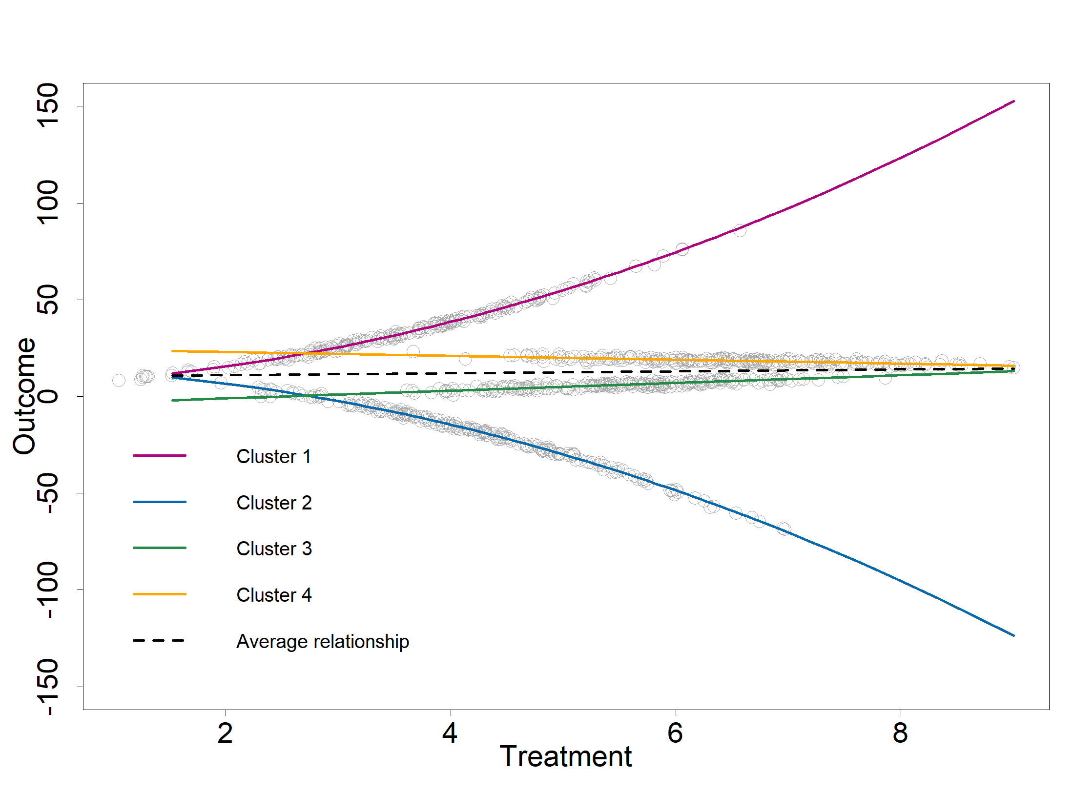
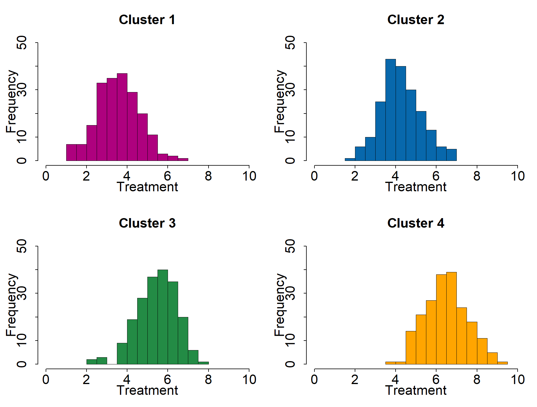
Figure 1: Relationship between treatment and outcome for all units and at the cluster level (left-hand side) and histogram of distribution of treatment within clusters (right-hand side)

In this scenario, we contend that the relationship averaged and estimated through a single ADRF lacks policy relevance, as it obscures the heterogeneity in the causal link between treatment and outcome. Indeed, this averaging process overlooks the existence of clusters where a strongly positive (or negative) relationship between treatment and outcome is evident. After generating the data, we first estimate the ADRF by using both the standard GPS approach of Hirano and Imbens, (2004) and the independence weights approach by Huling et al., (2024) to the whole set of 800 units, i.e., without taking into account the presence of clusters. The estimated ADRFs are displayed in Figure 2.

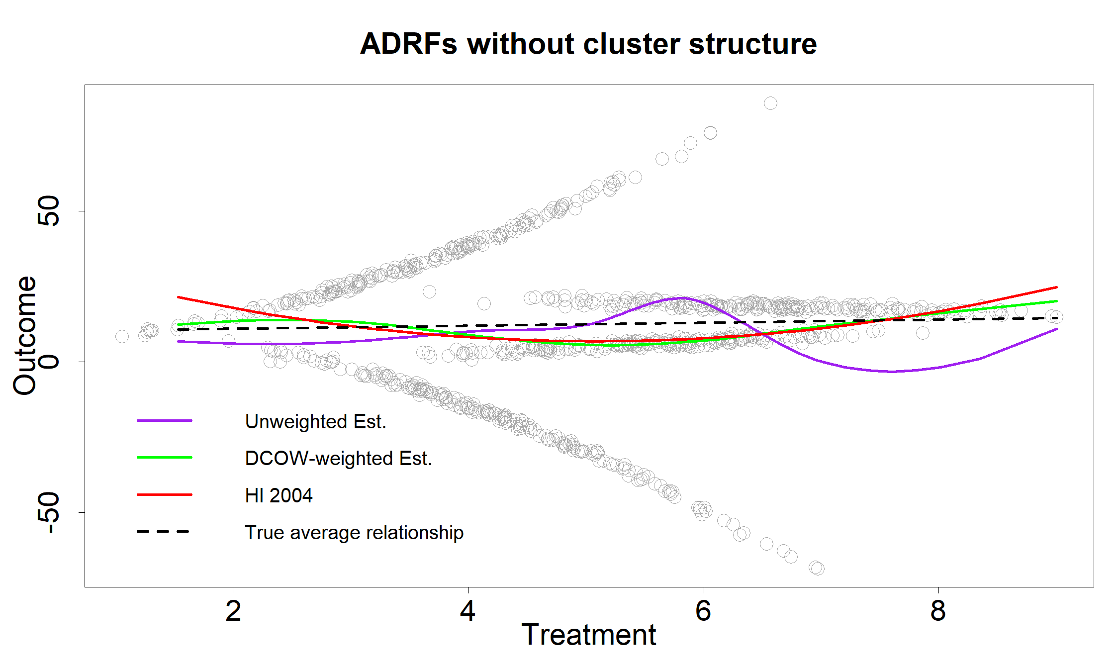
Figure 2: DRFs without cluster structure by using the Hirano and Imbens, (2004) approach and following Huling et al., (2024).

Note: True average relationship (dashed black line) represents the average of the four simulated relationships as in equation 2; HI2004 (red line) is the estimated ADRF by using the (Hirano and Imbens,, 2004) approach; Unweighted Est. (purple line) and DCOW-weighted Est. (green line) are the ADRFs estimated by using the (Huling et al.,, 2024) approach.

The ADRF of Hirano and Imbens, (2004) reveals a convex relationship, deviating significantly from the true simulated average relationship equal to the dashed line. Similarly, employing the approach proposed by Huling et al., (2024) leads to comparable challenges: the model’s fit indicates a non-linear relationship between the outcome and treatment, whereas the actual relationship is linear. This underscores the critical need to account for cluster structures: overlooking heterogeneity might lead to empirical analyses that lack policy relevance and may even produce biased estimates.

Let us assume the clustering structure to be known, so that we can estimate the ADRF using the Hirano and Imbens, (2004) approach within each of the known clusters. As shown in Figure 3, the estimated ADRFs (dashed black lines) perfectly resemble the true relationships (colored lines) within each cluster.

However, the setting discussed in Figure 3 is not realistic as the clusters are generally unknown. Hence, in Section 4.4 we will implement the Cl-DRF approach on these data and demonstrate that the method can successfully identify the number of clusters and the simulated relationships.

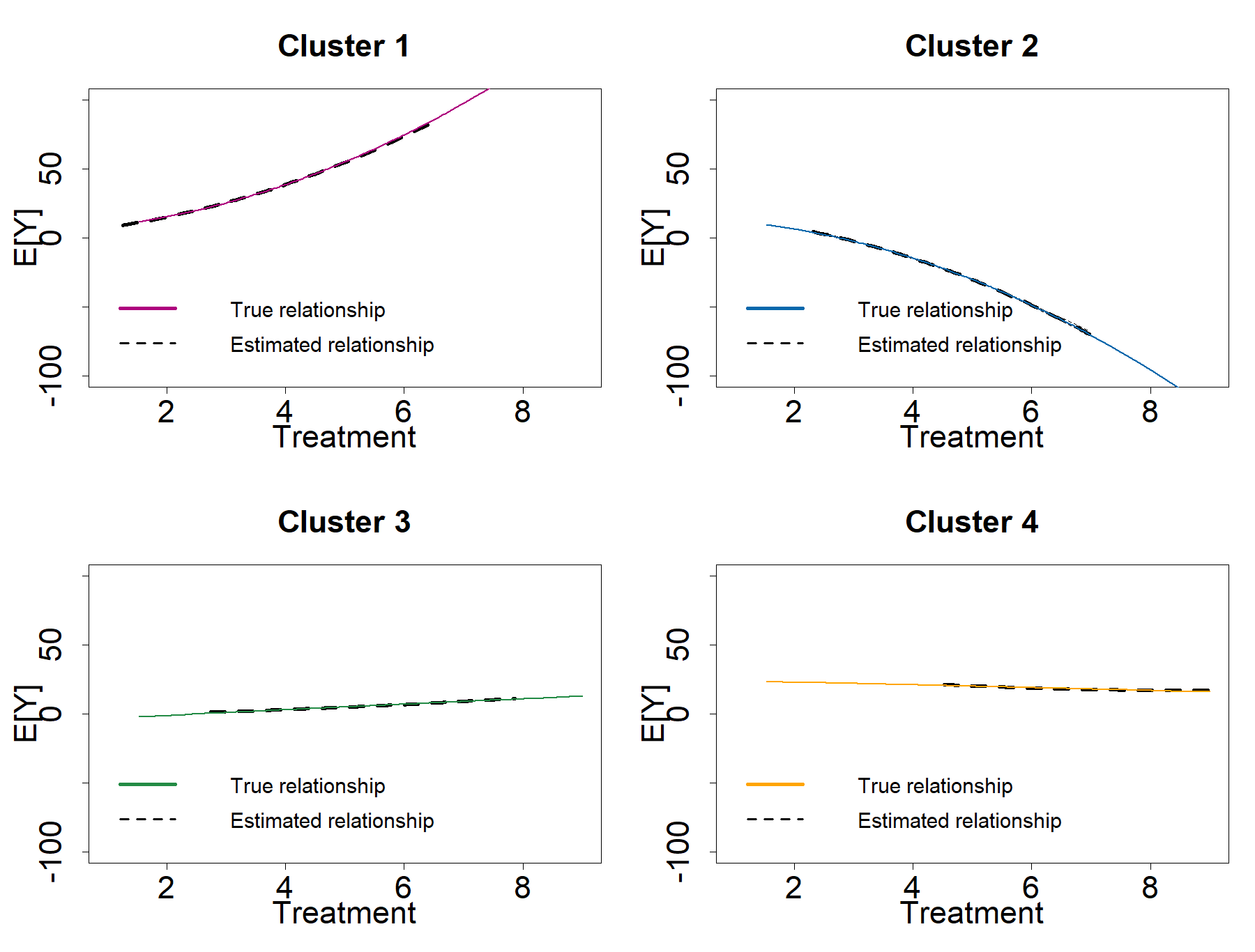
Figure 3: ADRFs estimated using the (Hirano and Imbens,, 2004) approach within each cluster, under the assumption that the cluster structure is known, compared to the true simulated relationships

Note: The colored lines represent the four simulated relationships for all values of treatment as in equation 2; the dashed black lines are the estimated ADRFs by using the (Hirano and Imbens,, 2004) approach.

3 Literature Review

In the context of policy evaluation, the simplification of treatment to binary terms and the assumption of homogeneous treatment effects across units have long represented the prevailing evaluation framework, aiding in the tractability and interpretation of empirical findings. However, in most circumstances, these simplifications fail to capture the complex nature of policy interventions, which can vary in intensity (e.g., firms receiving public subsidies are generally financed with different amounts), and produce heterogeneous effects even at a fixed treatment intensity, i.e., heterogeneous responses to a homogeneous treatment (e.g., training programs for the unemployed might assist some individuals in finding a job, while potentially disadvantaging others who might have secured a similar job more quickly without the training).

Addressing these limitations, two parallel strands of literature have emerged. The first body of research -reviewed in Section 3.1 -models the relationship between continuous treatment interventions and outcomes (e.g. Hirano and Imbens,, 2004, Fong et al.,, 2018, Wu et al.,, 2022), though it implicitly assumes homogeneous treatment effects. Another strand of literature examines the varied responses to the same treatment across different units (e.g. Athey and Imbens,, 2016, Wager and Athey,, 2018, De Chaisemartin and d’Haultfoeuille,, 2020, Callaway and Sant’Anna,, 2021) within the binary treatment framework and it is reviewed in Section 3.2.

3.1 Estimators for continuous treatment

While dichotomizing a continuous treatment variable is known to lead to information loss and potentially compromise data analysis quality (Fong et al.,, 2018), managing the inherent complexity of a continuous treatment framework poses significant challenges, especially in observational studies where the continuous treatment is not randomly assigned. A common approach to reducing confounding by observed variables is to use the propensity score generalized for the setting of continuous treatments (Hirano and Imbens,, 2004). This method aims to provide an unbiased estimate of the ADRF, which relates changes in the outcome variable to changes in treatment for the average unit. Each point of the ADRF represents the expected value of the potential outcome variable at a given treatment level of interest. The estimation process can be split in two steps:

1. The treatment model estimation, which produces the generalized propensity score (GPS), i.e., the conditional probability of being assigned to a particular level of treatment given a set of pre-treatment observed covariates. GPS can be seen as a balancing score.

2. The outcome model estimation, which uses the GPS to correct for treatment endogeneity in the outcome model. Adjusting for the GPS allows units with sufficiently similar characteristics but different treatment intensities to be compared, thus enabling the estimation of potential outcomes at different levels of treatment. By rebalancing the sample over the observed confounders, this approach allows unbiased estimation of the potential outcomes, provided that the assumptions of conditional independence and positivity hold (see below).

The difficulty of correctly specifying a conditional distribution is exacerbated by the increased dimension of the pre-treatment covariates to be controlled for, that is the confounders. To tackle this issue, Wu et al., (2022) adapt non-parametric matching techniques to the context of continuous treatment. An advantage of this approach is to separate the design phase from the analysis phase, ensuring the objectivity of the analysis since no post-treatment information is used during the design phase. Additionally, as misspecification of a conditional density model can be difficult to diagnose and assess, several studies have focused on directly estimating weights to reduce the correlation between marginal moments of (pre-treatment) covariates and the treatment. Approaches along this line of work include, among others, the generalized covariate balancing propensity score (CBPS) approach (Fong et al.,, 2018), covariate association eliminating weights (Yiu and Su,, 2018), entropy balancing weights (Tübbicke,, 2021) and independence weights (Huling et al.,, 2024). These approaches prioritize the direct estimation of weights over the explicit estimation and subsequent inversion of a conditional density, and they generally demonstrate superior empirical effectiveness compared to directly modelling the GPS (Huling et al.,, 2024).

All these estimators rely on the conditional independence (unconfoundedness) and the positivity assumptions (see Section 4.1 for more details). Considering the stringency of these assumptions, the usage of such estimators should be limited to contexts where the treatment intensity can be considered as quasi-randomly assigned, conditional on a set of pre-treatment observable characteristics, and where each unit could potentially receive a vast range of treatment intensities (Cerqua and Pellegrini,, 2024).

3.2 Estimators for heterogeneous treatment effects

It is well-established that units tend to respond differently to binary treatments (Athey and Imbens,, 2016). This highlights the increasing need for estimators that can assess heterogeneous treatment effects (HTE), focusing not just on average treatment effects but on capturing the diverse responses of different units to a binary treatment. Traditionally, HTE estimation involves repeating the analysis for different subgroups expected to exhibit heterogeneous effects based on prevailing theories (e.g., dividing between young and old individuals or between developed and underdeveloped geographical areas). However, this approach could lead to cherry-picking and multiple testing issues (Athey and Imbens,, 2016). In addition, it might miss the identification of the most relevant subgroups of units (Wager and Athey,, 2018). Recently, the emphasis has shifted towards data-driven estimation of HTE, with an approach that allows the algorithm to determine relevant features for estimating treatment effects through the application of machine learning techniques. The goal of this approach is to identify how the effects of a binary treatment vary across a population. These estimators adapt the objective function of well-known machine learning methods, such as decision trees or random forests, with the goal of exploring the heterogeneity of treatment effects relative to a certain set of covariates.

For example, the causal trees introduced by Athey and Imbens, (2016) are decision trees tailored to uncover the heterogeneity of treatment effects. In a causal tree, the aim is to achieve the best prediction of the treatment effect and to do this, the algorithm divides the data to minimize the heterogeneity of treatment effects within the leaves (i.e., the differences in potential outcomes), rather than minimizing the heterogeneity of observed outcomes within the leaves. A more complex approach is represented by the Generalized Random Forest (GRF) developed by Athey et al., (2019). The GRF iterates over random subsets of the data, constructing a causal tree for each subset. By combining numerous trees, the GRF produces robust and consistent treatment effect estimates under the conditional independence assumption.

While both strands of literature have developed effective estimators within their respective domains, they fall short in observational settings where treatment effects are heterogeneous across units even for the same treatment intensity, and the treatment is continuous. Applying these estimators in such contexts could lead to oversimplified policy recommendations, obscuring the complex impacts of policy measures. In the following section we introduce the Cl-DRF estimator, a method expressly developed for this evaluation context.

4 The Clustered Dose-Response-Function Estimator

4.1 The causal framework

The potential outcomes model for observational studies (Rubin,, 1974) is typically employed in binary contexts. Let $t_{i}$ be the binary treatment variable for unit $i$, and $y_{i}$ be the outcome variable for unit $i$. Here, $y_{i}(1)$ represents the potential outcome under treatment, while $y_{i}(0)$ denotes the potential outcome in the absence of treatment. Consequently, $y_{i}(1)-y_{i}(0)$ can be defined as the unit-level causal effect of a binary treatment. In a more general scenario with continuous treatment, $t_{i}$ assumes values within a real interval $\mbox{T}=[t_{min},t_{max}]$. Therefore, $y_{i}(t)$, where $t\in\mbox{T}$, signifies the outcomes for unit $i$ when exposed to treatment level $t$, varying within the set T. This is often referred to as the unit-dose response (Tübbicke,, 2021). So, in a continuous setting, we are interested in investigating the trajectory illustrating how $y_{i}(t)$ changes across relevant values of $t$. Usually, we are interested in population (or subgroup) causal effects, so we consider the expected potential outcomes $\mu(t)=E[y_{i}(t)]$, also called the average dose-response function (ADRF). Figure 4 shows the representation of the potential outcomes path for each unit with grey lines in a simulated example in which we know the actual dose-response function of each unit. The vertical lines at a generic level $t$ allow us to approximate the ADRF for each level $t$. Thus, the population ADRF is the solid black line.

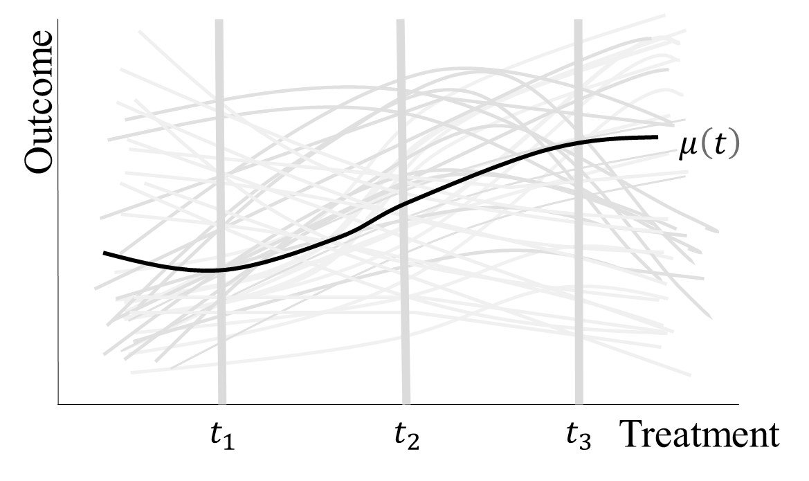
Figure 4: Average dose-response function. Example based on simulated data

In case of random assignment of the treatment intensity and a large number of observations, the average outcomes of units receiving distinct treatment intensities will deliver an unbiased estimate of the ADRF. Nevertheless, treatment intensity is very rarely randomly assigned in social sciences and most analyses focus on observational data, where there is no randomization of treatment. In most cases, the treatment depends on a set of covariates; therefore, we define the vector of observed pre-treatment covariates for each unit $i$ as $x_{i}$. With observational studies, we need to rely on some strong assumptions to obtain consistent estimates of the ADRF. Most available estimators for the ADRF in observational settings are based on the same set of assumptions; i) the no-interference assumption (Cox,, 1958) (aka consistency assumption), i.e., treatment received by one unit may affect the outcomes of other units; ii) the strong ignorability of treatment assignment assumption (aka unconfoundedness assumption), i.e., potential outcomes are independent of treatment conditional on covariates. This assumption is not testable, difficult to satisfy, and not generally applicable (Bia and Mattei,, 2012); and iii) the positivity assumption (aka overlap assumption) i.e., for every set of values of the covariates, there is a positive probability of receiving every possible treatment level. The latter assumption is crucial for the estimation of causal effects because it guarantees that there is sufficient overlap in the covariate distributions across different levels of the treatment, allowing for meaningful comparisons and generalization of causal effects across the population. In other words, the positivity assumption implies that for every combination of covariates within the range observed in the data, there must be a non-zero probability of receiving any given amount of the treatment. Such an assumption is arguably less tenable when the treatment is continuous because it is unlikely that every unit has a non-zero conditional density at every treatment value (Branson et al.,, 2023). Furthermore, even if positivity holds, propensity scores close to zero adversely affect the bias and variance of most estimators (Li et al.,, 2018). Violations of the positivity assumption arise when certain treatment levels are rarely or never observed within specific regions of the covariate space. This lack of overlap can lead to extrapolation and an unreliable estimate of the ADRF. In observational studies, researchers must be particularly vigilant for areas where overlap might be insufficient and consider techniques such as trimming or weighting to address imbalance (Branson et al.,, 2023).

Importantly, all surveyed estimators of continuous treatment rely on these assumptions and do not take into account the likely presence of treatment effects heterogeneity. This implies that when treatment effects are heterogeneous and the treatment is non-randomly assigned, the estimated ADRF is likely biased and not policy relevant. To overcome such limitations, we propose to model the continuous causal relationship between treatment intensity and the outcome, acknowledging and incorporating the likely heterogeneity of treatment effects. In this way, while we will still rely on the no-interference assumption, we can assume a weaker version of the latter two assumptions, requiring their validity exclusively within the defined clusters.

In fact, if we initially split the sample into $C$ clusters, chosen according to policy indications - e.g. small, medium and large firms - or following a data-driven procedure, we can estimate $C$ separated ADRFs that are meaningful at the cluster level, thus requiring the weak unconfoundedness and positivity assumptions to hold only within clusters. In the presence of HTE, these assumptions are less stringent compared to the requirements of weak unconfoundedness and positivity across all units. Moreover, the so-obtained ADRFs offer significantly enhanced informational value to policymakers.

4.2 The Cl-DRF algorithm

The concept behind Cl-DRF involves the estimation of cluster-specific ADRFs, which can be achieved through two approaches:

1. Theory-based approach. In this case, the sample is divided into clusters based on the specific features of the treatment under analysis or theoretical predictions, and then an ADRF is estimated within each cluster. For instance, Bia and Mattei, (2012) study the impact on employment of the amount of financial aid attributed to enterprises analysing small-sized firms and medium- or large-sized firms separately. Various approaches from the existing literature can be employed to estimate the ADRFs.

2. Data-driven approach

   In this case, clusters are not pre-determined, an algorithm is used to identify clusters and then estimate clustered ADRFs.

We deal with the latter case by employing a cluster-wise extension of the GPS approach of Hirano and Imbens, (2004) based on the assumption of unknown cluster membership, which builds on clustered regression techniques (e.g. see Bonhomme and Manresa,, 2015, Sugasawa,, 2021). This procedure enables us to simultaneously estimate the cluster structure of the data and the cluster-specific ADRF, which we refer to as the Cl-DRF estimator.

In the Cl-DRF estimator, the parameters determining the relationship between the received treatment and observed outcome are constrained to be the same for the units belonging to the same $c$-th cluster, and the clusters are estimated following an iterative procedure considering the similarity of the units in terms of their treatment-outcome relationship. The obtained clusters allow the construction of clustered ADRFs, which highlight different policy responses that cannot be identified with currently available estimators.

Let us consider the same notation of Section 2, where $n$ is the number of statistical units, $\mathbf{y}$ the outcome variable, $\mathbf{t}$ the observed treatment and $\mathbf{X}$ a set of covariates explaining the observed treatment. We then define $\boldsymbol{\kappa}_{c}=\text{diag}\left(\kappa_{1,c},\dots,\kappa_{i,c},\dots,\kappa_{n,c}\right)$ the $n$-dimensional diagonal matrix containing the binary membership of each $i$-th unit to the $c$-th cluster, such that $\kappa_{i,c}=1$ if the $i$-th unit belongs to the $c$-th cluster and zero otherwise.

Under the potential outcomes framework adapted to continuous treatment that we discussed in subsection 4.1 and considering the clustering structure, we need the following assumptions for identifiability:

Assumption 1: The no-interference assumption:

For each unit $i$, $t_{i}=t$ implies that $y_{i}=y_{i}(t)$. In other words, the treatment received by other units does not affect the potential outcomes of unit $i$. This assumption is the same as that used in all other estimators for continuous treatment described in Section 3.

Assumption 2: The unconfoundedness assumption within clusters:

For each $i\in c$, where $c=1\dots C$, $y_{i}(t)\perp\!\!\!\perp t\mid x_{i},c$.

Assumption 3: The positivity assumption within clusters:

For every possible value of $x_{i}$, the conditional probability density function of receiving any possible of $t\in T$ is positive within every cluster $c$, that is $f(t\mid x_{i})\geq v$ for all $x_{i}\in X$ for some constant $v>0$ in each cluster $c$.

Assumption 4: Correct cluster specification:

The clustering algorithm accurately partitions the data into clusters that correspond to the true underlying subpopulations.

This assumption ensures that within each cluster, the relationship between the treatment level and the outcome is correctly modelled and that the heterogeneity in treatment effects is appropriately captured.

Adapting the causal framework of Hirano and Imbens, (2004) to the presence of clusters, we define the relationship between the treatment and the covariates for the $i$-th unit in the cluster $c$ is

$$t_{i}\mid\mathbf{x}_{i},c\sim N\left(\boldsymbol{\beta}_{c}^{\prime}\mathbf{x}_{i},\sigma_{c}^{2}\right),\quad i=1,\dots,n;\quad c=1,\dots,C.$$ (3)

Now, given the generalization of the propensity score from binary exposure to continuous exposure as proposed by Hirano and Imbens, (2004) and given that in our setting the relationship between the outcome and the treatment is cluster-dependent, we define the conditional probability density functions of the treatment given covariates for the unit $i$ belonging to the $c$-th cluster as

$$r_{i}=\frac{1}{\sqrt{2\pi\sigma_{c}^{2}}}\exp\left[-\frac{1}{2\sigma_{c}^{2}}\left(t_{i}-\boldsymbol{\beta}^{\prime}_{c}\mathbf{x}_{i}\right)^{2}\right],$$ (4)

Under Assumptions 1-4, we can identify the clustered dose-response functions as

$$E[\mu(t,c)]=E\left[y_{i}\mid t_{i},r_{i},c\right]=f\left(t_{i},r_{i},\boldsymbol{\alpha_{c}}\right),$$ (5)

where $\boldsymbol{\alpha}_{c}$ is the vector of parameters for the $c$-th cluster and $f(\cdot)$ is a generic function.

In the case of linear specification for $f(\cdot)$, for instance, we get

$$E\left[y_{i}\mid t_{i},r_{i},c\right]=\alpha_{0,c}+\alpha_{1,c}t_{i}+\alpha_{2,c}r_{i}=\boldsymbol{\alpha}^{\prime}_{c}\mathbf{z}_{i},$$ (6)

with $\boldsymbol{\alpha}_{c}=[\alpha_{0,c},\alpha_{1,c},\alpha_{2,c}]$ and $\mathbf{z}_{i}=[1,t_{i},r_{i}]$, which can also include polynomial terms and/or interactions. We demonstrate that, as long as the functional form of $f(\cdot)$ is linear in its parameters, the vector $\boldsymbol{\alpha}_{c}$ can be estimated with OLS. Therefore, we assume $f(\cdot)$ to be a linear additive function that do not vary across clusters. In other words, we assume that all the $C$ clusters share the same functional form.

In order to estimate the clustered dose-response function, we need to follow three main steps: (i) estimating the cluster structure; (ii) updating the GPS according to such a structure; and (iii) modelling the conditional expectation of the outcome given the treatment and the GPS at the cluster level.

The Cl-DRF estimator is defined as the solution to the following minimization problem

$$\min J(\boldsymbol{\alpha}_{c},\boldsymbol{\kappa}_{c})=\min_{\boldsymbol{\alpha}_{c},\boldsymbol{\kappa}_{c}}\sum_{i=1}^{n}\sum_{c=1}^{C}\kappa_{i,c}\left(y_{i}-\boldsymbol{\alpha}^{\prime}_{c}\boldsymbol{z}_{i}\right)^{2},$$ (7)

under the constraint that $\sum_{c=1}^{C}\kappa_{i,c}=1$ and assuming that Equation (3) and Equation (4) hold, the optimal solutions are given in Proposition 1.

Proposition 1

Let us define $\mathbf{Z}=[\mathbf{z}_{1},\dots,\mathbf{z}_{i},\dots,\mathbf{z}_{n}]^{\prime}$. The optimal solutions for the objective function Equation (7) are given by

$$\boldsymbol{\alpha}_{c}=\left(\mathbf{Z}^{\prime}\boldsymbol{\kappa}_{c}\mathbf{Z}\right)^{-1}\mathbf{Z}\boldsymbol{\kappa}_{c}\mathbf{y},$$ (8)

for the parameters,

$$\kappa_{i,c}=\mathbf{1}\left[\left(y_{i}-\boldsymbol{\alpha}^{\prime}_{c}\boldsymbol{z}_{i}\right)^{2}\leq\left(y_{i}-\boldsymbol{\alpha}^{\prime}_{c^{\prime}}\boldsymbol{z}_{i}\right)^{2}\right],\quad\forall c\neq c^{\prime}$$ (9)

for the membership degree, and

$$r_{i}=I(\kappa_{i,c}=c)\frac{1}{\sqrt{2\pi\sigma_{c}^{2}}}\exp\left[-\frac{1}{2\sigma_{c}^{2}}\left(t_{i}-\boldsymbol{\beta}^{\prime}_{c}\mathbf{x}_{i}\right)^{2}\right],\quad\forall c=1,\dots,C.$$ (10)

for the GPS.

The proof of Proposition 1 is reported in A. The optimal solution needs to be solved iteratively. On one side, to find the optimal cluster-wise parameters $\boldsymbol{\alpha}_{c}$ we need to know the partition $\boldsymbol{\kappa}_{c}$. Furthermore, the knowledge of the partition $\boldsymbol{\kappa}_{c}$ is also needed for correctly updating the GPS estimate for the $c$-th cluster. We stress again that the GPS needs to be coherent with the cluster structure to meet its purpose of bias adjustment within each cluster. Given $\boldsymbol{\kappa}_{c}$, the GPS for each $c$-th cluster can be estimated using Equation (10). On the other side, the partition $\boldsymbol{\kappa}_{c}$ depends on the parameters $\boldsymbol{\alpha}_{c}$ and on the estimate of the GPS.

Therefore, we propose an algorithm that alternates an “assignment” step, where each unit is assigned to the cluster $c$ whose parameter minimizes the squared residuals, and an “update” step, where both the GPS and the parameters are estimated within each cluster. The proposed algorithm works as follows.

Let us assume a linear specification like in Equation (6). Given a suitable initial partition, $\boldsymbol{\kappa}^{(\text{init})}_{c}$, we have that the conditional expectation of the outcome given the treatment and the GPS estimate $\widehat{r}_{i}$, is modelled as a cluster-dependent function,

$$E\left[y_{i}\mid t_{i},\widehat{r}_{i},\boldsymbol{\kappa}^{(\text{init})}_{c}\right]=\alpha_{0,c}+\alpha_{1,c}t_{i}+\alpha_{2,c}\widehat{r}_{i},$$

where the parameters $\alpha_{0,c},\alpha_{1,c}$ and $\alpha_{2,c}$ are estimated by OLS Equation (8), that is,

$$\widehat{\boldsymbol{\alpha}}_{c}\left(\boldsymbol{\kappa}^{(\text{init})}_{c},\widehat{r}_{i}\right) =\underset{\boldsymbol{\alpha}_{c}}{\operatorname{argmin}}\sum_{i=1}^{n}\kappa^{(\text{init})}_{i,c}\left(y_{i}-\alpha_{0,c}-\alpha_{1,c}t_{i}-\alpha_{2,c}\widehat{r}_{i}\right)^{2}=$$

$$=\left(\mathbf{Z}^{\prime}\boldsymbol{\kappa}^{(\text{init})}_{c}\mathbf{Z}\right)^{-1}\mathbf{Z}\boldsymbol{\kappa}^{(\text{init})}_{c}\mathbf{y}.$$

Given these initial estimates, each $i$-th unit is re-assigned to the cluster $c$ minimizing its squared residuals, that is,

$$\widehat{\kappa}_{i,c}\left(\widehat{\boldsymbol{\alpha}}_{c},\widehat{r}_{i}\right)=\mathbf{1}\left[\left(y_{i}-\widehat{\alpha}_{0,c}-\widehat{\alpha}_{1,c}t_{i}-\widehat{\alpha}_{2,c}\widehat{r}_{i}\right)^{2}\leq\left(y_{i}-\widehat{\alpha}_{0,c^{\prime}}-\widehat{\alpha}_{1,c^{\prime}}t_{i}-\widehat{\alpha}_{2,c^{\prime}}\widehat{r}_{i}\right)^{2}\right],$$

$\forall c^{\prime}\neq c$. Given the so-obtained clustering membership $\widehat{\boldsymbol{\kappa}}_{c}$, the GPS estimate for the $i$-th unit $\widehat{r}_{i}$ is updated with Equation (10) to accommodate for the new cluster structure found with Equation (9). In particular, we estimate the parameters $\widehat{\boldsymbol{\beta}}_{c}$ and $\widehat{\sigma}^{2}_{c}$ with maximum likelihood within each cluster. Then, the parameters of the outcome model, $\boldsymbol{\alpha}_{c}$, are re-estimated by minimizing the sum of squared residuals as in Equation (8), but using the membership $\hat{\boldsymbol{\kappa}}_{c}$ instead of $\boldsymbol{\kappa}^{(\text{init})}_{c}$. The same scheme applies if polynomials and/or interaction terms of the treatment and GPS are considered.

The iterative process described above alternates between the assignment, the GPS update and the parameter estimation steps until convergence, ensuring that the clustering structure accurately reflects the relationship between the outcome and the treatment and that the GPS is coherent with the cluster structure. Algorithm 1 provides a detailed explanation of the iterative procedure of the Cl-DRF estimator.

At the end of such a procedure, which stops when no significant update in the clustering structure is found, we obtain at the same time the clustering assignment of the $n$ units in the $C$ clusters and the within-cluster relationship needed for the computation of the $C$ ADRFs. Indeed, once the partition of the units into $C$ clusters is found, we can estimate the ADRFs within each cluster by using the same parameters of the last iteration. Other estimation approaches (e.g., independence weights) may also be easily implemented given the clustering structure.

Input : Outcome $\mathbf{y}$, Treatment $\mathbf{t}$, Covariates $\mathbf{X}$, Number of clusters ($C$), Maximum iterations (max.itr)

Output : Final cluster assignments, Clustered regression results

Initialize the algorithm providing an initial cluster assignments $\boldsymbol{\kappa}^{(\text{init})}_{c}$ and GPS estimate $\widehat{r}_{i}$; 

while $\boldsymbol{\kappa}^{(s)}_{c}\neq\boldsymbol{\kappa}^{(s-1)}_{c}$ and $s\leq\text{max.itr}$ do

       // Update estimates

       for c in 1:C do

             $\boldsymbol{\alpha}^{(s)}_{c}=\left(\mathbf{Z}^{(s-1)^{\prime}}\boldsymbol{\kappa}^{(s-1)}_{c}\mathbf{Z}^{(s-1)}\right)^{-1}\mathbf{Z}^{(s-1)}\boldsymbol{\kappa}^{(s-1)}_{c}\mathbf{y}.$

       end for

      

      // Update clustering

       for i in 1:n do

             $\kappa^{(s)}_{i,c}=\mathbf{1}\left[\left(y_{i}-\boldsymbol{\alpha}^{(s)^{\prime}}_{c}\boldsymbol{z}^{(s-1)}_{i}\right)^{2}\leq\left(y_{i}-\boldsymbol{\alpha}^{(s)^{\prime}}_{c^{{}^{\prime}}}\boldsymbol{z}^{(s-1)}_{i}\right)^{2}\right]$

       end for

      

      // Update GPS

       for c in 1:C do

             $r^{(s)}_{i}=I(\kappa^{(s)}_{i,c}=c)\frac{1}{\sqrt{2\pi\widehat{\sigma}_{c}^{2}}}\exp\left[-\frac{1}{2\widehat{\sigma}_{c}^{2}}\left(t_{i}-\widehat{\boldsymbol{\beta}}^{{}^{\prime}}_{c}\mathbf{x}_{i}\right)^{2}\right],$

       end for

      

      $\mathbf{z}^{(s)}_{i}=[1,t_{i},r^{(s)}_{i}]$;

      

      $\mathbf{Z}^{(s)}=[\mathbf{z}^{(s)}_{1},\dots,\mathbf{z}^{(s)}_{i},\dots,\mathbf{z}^{(s)}_{n}]$;

      

      $s\leftarrow s+1$;

      

end while

Algorithm 1 Cl-DRF algorithm

4.3 Choosing the number of clusters

The Cl-DRF builds on the $k$-means regression methodology and it shares two of its key features. First, Cl-DRF assumes that at least two clusters exist, that is, $C\geq 2$. Second, to use the Cl-DRF we need to specify the number of clusters $C$ in advance. In what follows, we discuss an iterative approach for selecting a suitable number of clusters.

For selecting the number of clusters $C$, we propose a simple but effective rule based on the following BIC-like criterion (e.g. see Sugasawa,, 2021)

$$\operatorname{IC}(C)=-2\log p\left(y_{i}\mid\mathbf{z}_{i},\widehat{\boldsymbol{\alpha}}_{c}\right)+\zeta_{n}\operatorname{dim}(\widehat{\boldsymbol{\alpha}}_{c}).$$ (11)

Under the assumption of i.i.d. Gaussian errors, we assume $p(\cdot)$ to be the Gaussian density, $\zeta_{n}$ is a constant depending on the sample size $n$ and $\operatorname{dim}(\widehat{\boldsymbol{\alpha}}_{c})$ denotes the number of parameters $\widehat{\boldsymbol{\alpha}}_{c}$ in the $c$-th cluster, which depends on the functional specification of the treatment-outcome model. Indeed, including polynomial terms of treatment and GPS and/or their interaction terms make the value of $\operatorname{dim}(\boldsymbol{\alpha}_{c})$ increase. We let $\zeta_{n}=\log n$ and compute the value of $\operatorname{IC}(c)$ for $c=2,\dots,C_{\max}$. We then select the suitable value of $C$ with the Elbow method (Zhao et al.,, 2008). By letting $J(0)$ the objective function value is obtained with a baseline model without clusters. Given $C_{\max}$ maximum number of clusters, we define $J(c)$ as the value of the objective function with $c$ $(c=2,\dots,C_{\max})$ clusters. We automatically detect the elbow at $c$ such that the difference between $J(c)$ and the value of the straight line connecting the extreme points $J(0)$ and $J(C_{\max})$ is maximized. The objective function to maximize is, therefore, (Morgado et al.,, 2023)

$$C=\arg\min_{c}\left[\frac{J(0)}{C_{\max}}\cdot c+J(c)\right].$$ (12)

The optimal solution to this problem is taken as the optimal number of clusters. The simulations in Section 5 show that this approach leads to very high accuracy in the selection of the number of clusters $C$.

4.4 Again on the motivating example

Let us consider the motivating example discussed in Section 2. We now apply the Cl-DRF estimator and the results are shown in Figure 2. To apply the Cl-DRF estimator we need to choose the number of clusters $C$. Considering different values in the set $C=\{2,3,4,5,6,7\}$, we compute the values of the BIC-like criterion as shown in Equation (11). It can be verified that an elbow is detected at $C=4$, which is the true number of clusters. The Rand Index, which provides a measure of agreement between the obtained partition with the proposed Cl-DRF estimator and the true one, is equal to 0.98, which suggests an almost perfect identification of the simulated clusters. As shown in Figure 6, the ADRFs reproduced with the Cl-DRF estimator (dashed black line) are very close to the true ADRFs (colored lined), demonstrating the efficacy of the Cl-DRF estimator in this example.

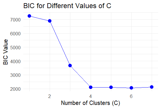
Figure 5: BIC values Equation (11) for different values of $C$, in the set $C=\{2,3,4,5,6,7\}$. We choose $C$ with the Elbow criterion. We detect an elbow for $C=4$.

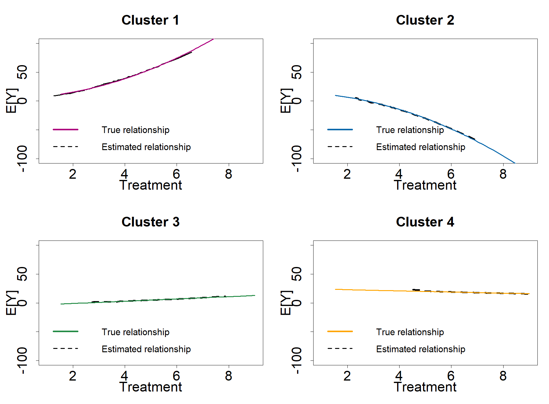
Figure 6: DRFs estimated using the Cl-DRF approach compared to the true simulated relationships

Note: The colored lines represent the four simulated relationships for all values of treatment as in equation 2; the dashed black lines are the estimated DRFs by using the Cl-DRF approach.

5 Simulation study

In what follows we consider the results of a simulation study to evaluate the properties of the proposed Cl-DRF. In particular, we evaluate the appropriateness of the approach discussed in Section 4.3 for choosing the number of clusters $C$. Moreover, we evaluate the ADRF reconstruction properties of the Cl-DRF estimator.

For this aim, we consider $1000$ replications consisting of datasets with two different sample sizes, that is $n=400$ and $n=800$ units, that are clustered into $C$ equally sized groups. We first consider the results of the experiment with $C=4$ but we also consider simulation results with a lower and larger number of clusters, $C=3$ and $C=5$. In each of the $C$ clusters, we simulate two covariates $\mathbf{x}_{i}=[x_{i1},x_{i2}]$ according to the following relationships

$$t_{i}\mid\mathbf{x}_{i},c\sim N\left(\boldsymbol{\beta}^{\prime}_{c}\mathbf{x}_{i},1\right),$$ (13)

where $\boldsymbol{\beta}^{\prime}_{c}\neq\boldsymbol{\beta}^{\prime}_{c^{\prime}}$, $\forall c^{\prime}\neq c$. Then, we simulate the outcome variable as a function of the simulated treatment and assume the following within-cluster relationships

$$y_{i}=\alpha_{0,c}+\alpha_{1,c}t_{i}+e_{i},$$ (14)

where $e_{i}\sim N(0,1)$, $\forall i$. Moreover, we assume that the treatment outcome relationships are different in the $C$ clusters, that is, $\alpha_{0,c}\neq\alpha_{0,c^{\prime}}$ and $\alpha_{1,c}\neq\alpha_{1,c^{\prime}}$ $\forall c^{\prime}\neq c$. We also provide simulation results under the assumption of random treatment, that is, $t_{i}\sim N(\mu,\sigma^{2})$ where $\mu_{i}=\mu$ and $\sigma^{2}_{i}=\sigma^{2}$ $\forall i=1,\dots,n$. The results of this additional simulation setting are shown in C.

For the main simulations, we consider the case where, in line with the motivating examples, the true number of clusters is $C=4$. We assume $x_{1i}\sim U[0,0.4]$ and $x_{2i}\sim U[0,0.5]$ for the Cluster 1, $x_{1i}\sim U[0.2,0.6]$ and $x_{2i}\sim U[0.3,0.6]$ for the Cluster 2, $x_{1i}\sim U[0.5,0.8]$ and $x_{2i}\sim U[0.5,0.9]$ for the Cluster 3 and $x_{1i}\sim U[0.7,1]$ and $x_{2i}\sim U[0.7,1]$ for the Cluster 4, where $U[a,b]$ denotes the continuous uniform distribution with support $[a,b]$. Moreover, for the relationships Equation (13) we simulate the following cluster-specific parameters $\boldsymbol{\beta}_{1}=[1.7,2]$, $\boldsymbol{\beta}_{2}=[1.2,1.2]$, $\boldsymbol{\beta}_{3}=[0.7,0.5]$ and $\boldsymbol{\beta}_{4}=[0.5,0.2]$. Then, we simulate the outcome variable as a linear function of the simulated treatment Equation (14) and assume the following within-cluster relationships

$$y_{i}=\begin{cases}\@add@centering\centering 5+t_{i}+e_{i}&\text{ for }c=1\\ 15-2t_{i}+e_{i}&\text{ for }c=2\\ -5-0.01t_{i}+e_{i}&\text{ for }c=3\\ 25+2t_{i}+e_{i}&\text{ for }c=4\\ \end{cases}$$ (15)

where $e_{i}\sim N(0,1)$, $\forall i$.

Before applying the Cl-DRF, we need to choose the number of clusters $C$. Following Section 4.3, we compute the BIC criterion for different values of $C$ and choose the optimal number of clusters using the data-driven approach discussed in Equation (12), which is based on the Elbow criterion. Figure 7 shows the boxplots of the clustering accuracy, computed with the Rand Index (Figure 7(a)), and of the selected number of clusters $C$ (Figure 7(b)) over the $1000$ simulations.

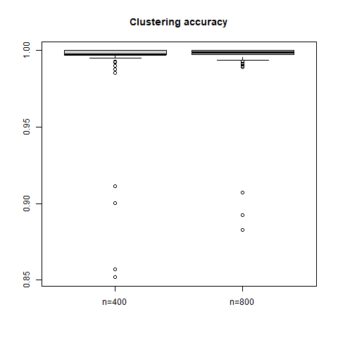
(a) Rand Index for the partitions obtained using the Cl-DRF estimator.

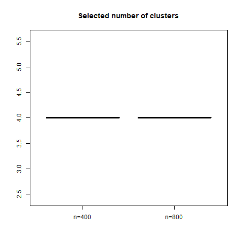
(b) Selected number of clusters.

Figure 7: Boxplot showing the clustering accuracy, computed with the Rand Index, over the $1000$ simulations. The Elbow criterion with the BIC criterion is used for selecting $C$. Simulated scenario with $C=4$.

The results in Figure 7 highlight that we choose the correct number of clusters in all the $1000$ simulations. As a result, the average Rand Index is close to 1, thus suggesting perfect cluster reconstruction properties of our Cl-DRF estimator. In other words, Figure 7 suggests that the approach adopted for the number of clusters selection is appropriate and that, if the correct number of clusters is specified, the Cl-DRF reconstructs the ground truth. This result holds for both scenarios with $n=400$ and $n=800$, although the variability of the results in the setting with $n=800$ is lower compared with $n=400$ and the average Rand Index is slightly higher. Next, we evaluate the property of the Cl-DRF approach in estimating relevant ADRFs from the policy perspective. The average ADRF, for each of the $C=4$ clusters, in the case of $n=400$ is shown in Figure 8, while the case of $n=800$ is shown in Figure 9.

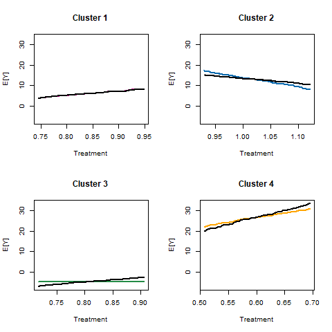
Figure 8: DRFs estimated using the Cl-DRF approach compared to the true simulated relationships. Simulated scenario with $C=4$ and $n=400$.

Note: The colored lines represent the four simulated relationships for all values of treatment as in equation 15; the black lines are the estimated DRFs by using the Cl-DRF approach.

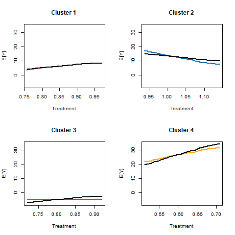
Figure 9: DRFs estimated using the Cl-DRF approach compared to the true simulated relationships. Simulated scenario with $C=4$ and $n=800$.

Note: The colored lines represent the four simulated relationships for all values of treatment as in equation 15; the black lines are the estimated DRFs by using the Cl-DRF approach.

In summary, the Cl-DRF estimator results in a perfect overlap of the ADRF for Cluster 1, whereas the ADRFs for the other clusters are not reconstructed perfectly. However, from the policy perspective, we find that the ADRFs estimated with the Cl-DRF estimator are relevant and provide a reliable picture of the differences within each cluster in terms of dose-response relationship. Indeed, we correctly reconstruct that the treatment has a positive relationship with the outcome for the units belonging to Cluster 1 and Cluster 4, while the relationship is negative for those placed in Cluster 2. We also correctly find that the treatment-outcome relationship is near zero for units in Cluster 3.

We also consider simulations with $C=5$ and $C=3$. The results, shown in B, are in line with those obtained for $C=4$. Indeed, we found that the Elbow criterion in Equation (12) allows selecting the correct number of clusters and that the clustering accuracy measured in terms of average Rand Index is near to unity.

6 Empirical application

In this section we provide an empirical illustration of the Cl-DRF estimator by analyzing the causal impact of the European Union (EU) regional policy (aka Cohesion Policy), i.e., the most extensive regional policy in terms of breadth, amount of resources involved and duration.

6.1 Background

While the bulk of the Cohesion Policy aims at supporting the growth processes of the poorest EU regions, it also finances projects in richer regions. This results in a situation where all regions receive some treatment, but the intensity of treatment is vastly heterogeneous in the amount of funds. For instance, from 1994 to 2006, the North-Holland region received an annual average per capita transfer close to €9, whereas the Região Autónoma dos Açores (PT) received €773, almost 85 times more (Cerqua and Pellegrini,, 2018). The Cohesion Policy assignment process suggests that regions receiving large amounts of funds are fundamentally different from those receiving few funds. Estimating a single ADRF under these circumstances could result in comparisons between areas with significant disparities in pre-treatment economic growth, per capita GDP, investment rates, and other relevant factors.

Previous literature has already analyzed and demonstrated the presence of heterogeneity of the Cohesion Policy effects with respect to the intensity of treatment (Becker et al.,, 2012, Cerqua and Pellegrini,, 2018). These studies show that transfers enable faster economic growth in the recipient regions, but the transfer intensity exceeds the aggregate efficiency maximizing level. At the same time, other studies (Becker et al.,, 2013, Rodríguez-Pose and Garcilazo,, 2015) have found that the effect of public transfers on economic growth depends on the absorptive capacity of recipient regions (proxied by human capital endowments and quality of institutions). Considering these findings together, they suggest that one should ideally account for both the heterogeneity of treatment in terms of transfer intensity and the heterogeneous responses to the same amount of funds.

6.2 Data

In this analysis we will focus on the relationship between EU funds and economic growth for the period from 1994 to 2015. The main data source is the Annual Regional Database of the European Commission’s Directorate General for Regional and Urban Policy (ARDECO) dataset, which provides comprehensive socio-economic and demographic data for regions across the European Union.

In particular, we will focus on the NUTS-2 regional level and use the GDP per capita adjusted at Purchasing Power Standard (PPS) compound annual growth rate from 1994 to 2015 as the dependent variable.

We will control for the 1994 values of the following variables: i) per capita GDP in PPS; ii) population density; iii) share of gross value added (GVA) in the primary sector; iv) average yearly hours worked per employee; v) average yearly compensation per employee; vi) workplace employment rate. Another key variable for our analysis is the yearly estimate of the amount of funds per capita received over the programming period (see Cerqua and Pellegrini, (2023)) that will be used as the treatment intensity variable.

Table 1: Descriptive statistics

	Mean	SD	Min	Max
Yearly GDP per capita growth rate	2.54%	0.66%	0.52%	5.94%
Yearly EU funds per capita (1994-2015)	€78.39	€92.70	€7.89	€425.28
GDP per capita in PPS in 1994	€17,599	€6,383	€8,564	€78,912
Population density in 1994	455.12	1,098.42	3.18	8,414.19
Share GVA primary sector in 1994	0.029	0.031	0.001	0.178
Avg hours worked per empl. in 1994	1,718.80	213.83	607.23	2,359.61
Avg compensation per empl. in 1994	€20,057.09	€6,567.75	€4,758.00	€39,916.34
Workplace employment rate in 1994	42.09%	9.98%	27.32%	145.18%

6.3 Results

In this section we use the traditional methods of (Hirano and Imbens,, 2004), (Huling et al.,, 2024) and the Cl-DRF estimator to estimate the causal continuous relationship between EU funds and economic growth. The corresponding ADRFs are reported in Figure 10 for the first two methods and Figure 11 for the Cl-DRF estimator.

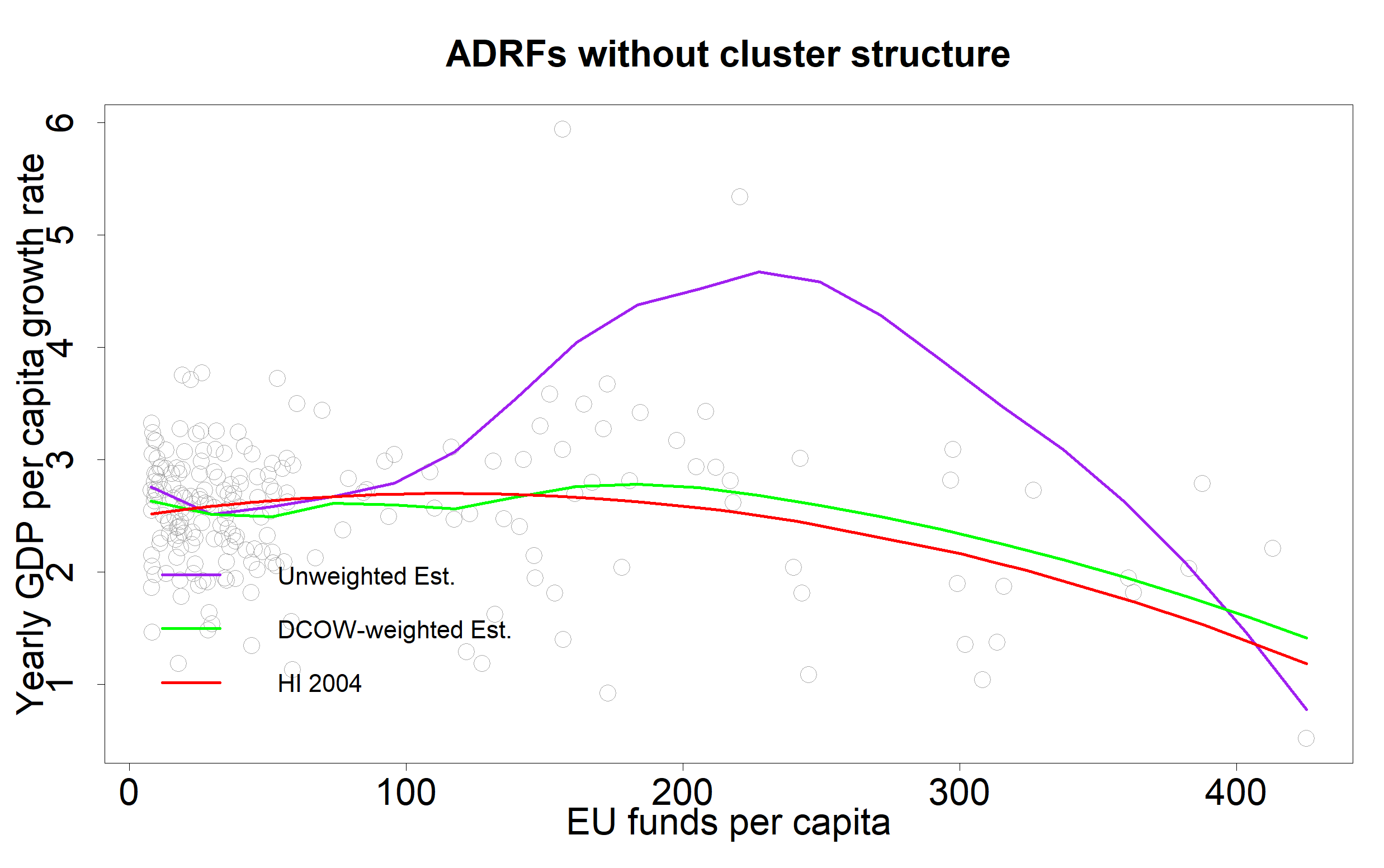
Figure 10: Note: HI2004 (red line) is the estimated ADRF by using the (Hirano and Imbens,, 2004) approach; Unweighted Est. (purple line) and DCOW-weighted Est. (green line) are the ADRFs estimated by using the (Huling et al.,, 2024) approach.

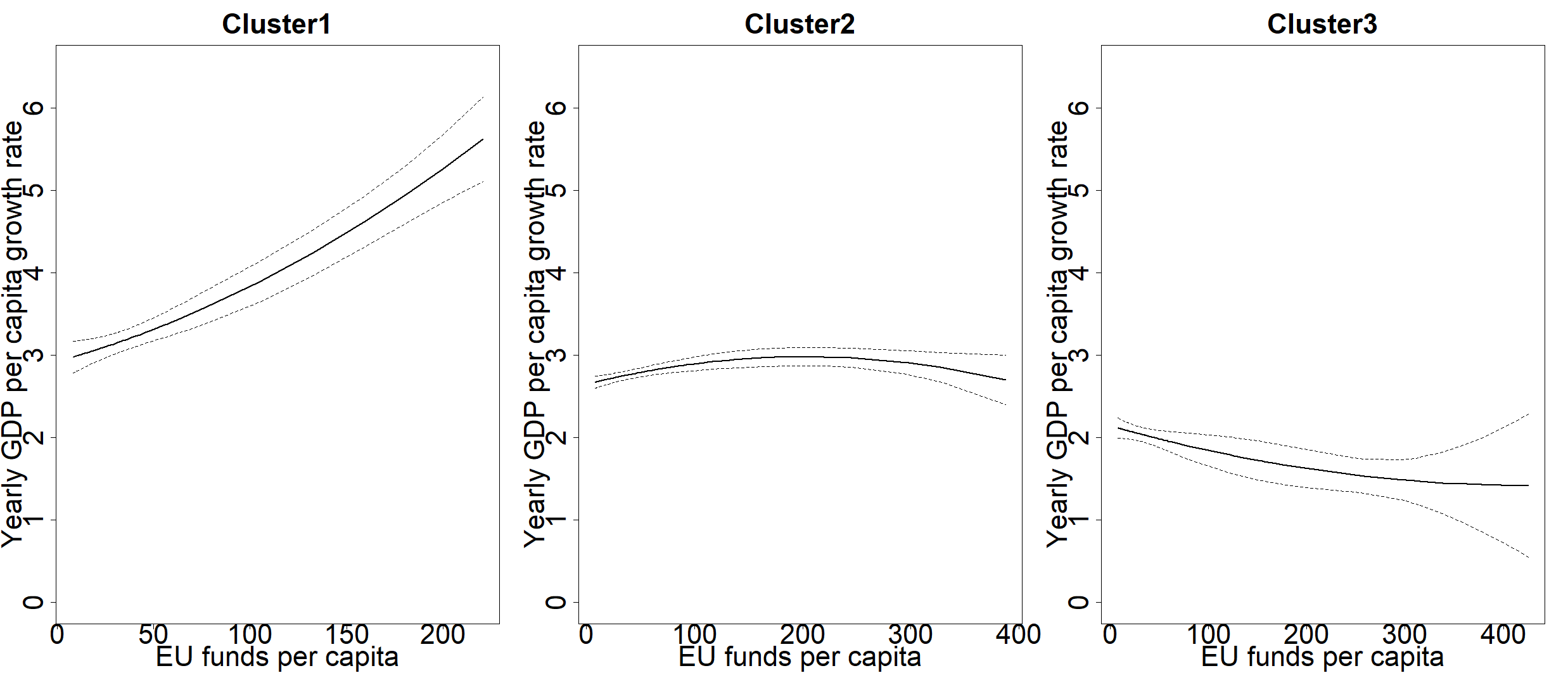
Figure 11: Clustered ADRFs with the proposed approach

Figure 10 shows a slightly positive relationship between EU funds and economic growth, which flattens out for regions receiving more than 100 euros per capita per year and turns even negative for the most subsidized regions. Not surprisingly, this finding is in line with the findings of (Becker et al.,, 2012) who have used the GPS estimator to study the same relationship over the two programming periods 1994-1999 and 2000-2006.

On the other hand, looking at Figure 11, we see that the Cl-DRF algorithm selects three clusters: Cluster 2 exhibits a relationship between treatment intensity and economic growth similar to that reported in Figure 10. In contrast, Cluster 1 shows a steep positive relationship between funds and growth, while regions in Cluster 3 display a slight negative relationship. Notably, the common support of the first cluster is much smaller and does not include any of the most subsidized areas. Importantly, the difference between the ADRFs reported in Figure 10 and those in Figure 11 suggests that the lack of consideration for the likely presence of HTE in the case of continuous treatments might lead to biased estimates and, consequently, to incorrect policy recommendations. For instance, our analysis reveals that, at least for some of the wealthiest EU regions in Cluster 1, there is no evidence supporting the hypothesis that a maximum funding threshold exists beyond which additional resources fail to stimulate further economic growth (see (Becker et al.,, 2012, Cerqua and Pellegrini,, 2018)).

Looking at the composition of the clusters displayed in Figure 12, we see that Cluster 1 includes regions from Ireland, Southern Germany, and Southern England, while Cluster 2 predominantly consists of regions in Spain, Northern Germany, the Netherlands, Sweden, and Finland. Lastly, Cluster 3 is composed of many French regions as well as nearly all regions in Italy and Greece. These latter countries were among the hardest hit during the Great Recession, which may explain the counterintuitive finding that higher EU funding led to less growth in these regions. Indeed, particularly during the years 2008-2015, regional inequalities in Greece and Italy widened ((Fingleton et al.,, 2015)), despite the larger influx of EU funds to their least developed regions.

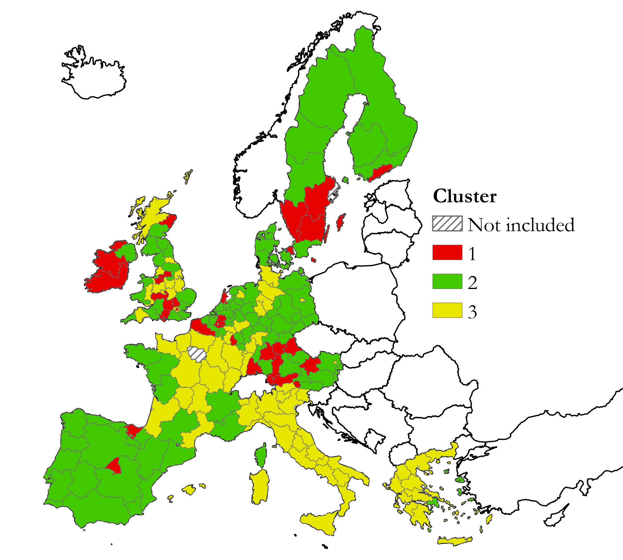
Figure 12: Map of the three clusters

Note: To limit the issue of extrapolation, we have trimmed from the analysis four regions, the two with the highest/lowest treatment intensity.

7 Conclusions

The study highlights the challenges of estimating a single ADRF in the presence of continuous treatment and heterogeneity among treated units in the treatment-outcome relationship. We demonstrate that, under these circumstances, available estimators do not allow for an unbiased estimation of the ADRF and do not provide separate estimations for different clusters of units.

To address this gap, we propose the Cl-DRF estimator. By integrating clustering methodologies into continuous treatment analysis, the Cl-DRF acknowledges the potential differential impacts of covariates and accounts for spatial or clustered units. Instead of estimating a single ADRF, it estimates an ADRF for each cluster of units, providing more detailed information to policymakers. This integrative approach not only reflects the increasing complexity of policy measures but also addresses the growing demand for more advanced tools in policy evaluation, as highlighted in recent scholarly discussions (Wu et al.,, 2022). The Cl-DRF offers several advantages: it requires a weaker version of the conditional independence and positivity assumptions, increases interpretability, reduces p-hacking, and accommodates data-driven clustering. To illustrate the potential of the Cl-DRF estimator, we presented a simulation study and an empirical analysis on the effects of the Cohesion Policy in the EU-15 NUTS-2 regions.

Our research aims to enhance the methodological arsenal available for causal inference in the presence of continuous treatments, paving the way for more nuanced and accurate analyses in social sciences and beyond.

In a future version of the paper, we intend to enhance our findings in two key ways. Firstly, our simulation design in Section 5 currently presumes no misspecification between treatment and outcome, which might be unrealistic. We plan to expand our simulations to include scenarios where some ADRFs are misspecified, as initially suggested in Sections 2 and 4.4. Secondly, in line with previous studies on clusterwise regression (e.g. see Bonhomme and Manresa,, 2015, Sugasawa,, 2021), we presume a clustering structure which we then estimate using a data-driven approach. Nevertheless, validating this clustering assumption in the context of continuous treatment remains an open question. We believe that the non-parametric test proposed by Dette and Neumeyer, (2001) could effectively address this issue, although further research is required to explore this possibility thoroughly.

Appendix A Proof of Proposition 1

We recall that the Cl-DRF estimator is defined as the solution to the following minimization problem

$$\min J(\boldsymbol{\alpha}_{c},\boldsymbol{\kappa}_{c})=\min_{\boldsymbol{\alpha}_{c},\boldsymbol{\kappa}_{c}}\sum_{i=1}^{n}\sum_{c=1}^{C}\kappa_{i,c}\left(y_{i}-\boldsymbol{\alpha}^{\prime}_{c}\boldsymbol{z}_{i}\right)^{2},$$ (16)

under the constraint that $\sum_{c=1}^{C}\kappa_{i,c}=1$ and under the assumptions Equation (3) and Equation (4), needed for GPS adjustment. In what follows we show that the optimal solutions are those shown in Proposition 1, that is, Equation (8), Equation (9) and Equation (10).

Proof. The solutions can be obtained by considering the following Lagrangian function

$$\mathcal{L}\left(\boldsymbol{\alpha}_{c},\kappa_{i,c},\lambda\right)=\sum_{i=1}^{n}\sum_{c=1}^{C}\kappa_{i,c}\left(y_{i}-\boldsymbol{\alpha}^{\prime}_{c}\mathbf{z}_{i}\right)^{2}+\lambda\left(\sum_{c=1}^{C}\kappa_{i,c}-1\right).$$ (17)

To find the solution for the parameters, we set the partial derivative of the Lagrangian with respect to $\boldsymbol{\alpha}_{c}$ equal to zero

$$\frac{\partial\mathcal{L}\left(\boldsymbol{\alpha}_{c},\kappa_{i,c},\lambda\right)}{\partial\boldsymbol{\alpha}_{c}}=0,$$

that reduces to finding the solution to the problem

$$\min J\left(\boldsymbol{\alpha}_{c},\boldsymbol{\kappa}_{c}\right)=\underset{\boldsymbol{\alpha}_{c}}{\operatorname{argmin}}\sum_{i=1}^{n}\kappa_{i,c}\left(y_{i}-\boldsymbol{\alpha}^{\prime}_{c}\mathbf{z}_{i}\right)^{2}.$$

In the matrix form, it can be written as

$$\frac{\partial(\mathbf{y}-\mathbf{Z}\boldsymbol{\alpha}_{c})^{\prime}\boldsymbol{\kappa}_{c}(\mathbf{y}-\mathbf{Z}\boldsymbol{\alpha}_{c})}{\partial\boldsymbol{\alpha}_{c}}=\mathbf{Z}^{\prime}\boldsymbol{\kappa}_{c}(\mathbf{y}-\mathbf{Z}\boldsymbol{\alpha}_{c})=0.$$

By expanding this equation, we obtain

$$\mathbf{Z}^{\prime}\boldsymbol{\kappa}_{c}\mathbf{y}=\mathbf{Z}^{\prime}\boldsymbol{\kappa}_{c}\mathbf{Z}\boldsymbol{\alpha}_{c},$$

and by solving for $\boldsymbol{\alpha}_{c}$ we finally get

$$\boldsymbol{\alpha}_{c}=\left(\mathbf{Z}^{\prime}\boldsymbol{\kappa}_{c}\mathbf{Z}\right)^{-1}\mathbf{Z}\boldsymbol{\kappa}_{c}\mathbf{y},$$

which is Equation (8). To find the optimal cluster assignment we take the first derivative of the Lagrangian with respect to $\kappa_{i,c}$, that is,

$$\frac{\partial\mathcal{L}\left(\boldsymbol{\alpha}_{c},\kappa_{i,c},\lambda\right)}{\partial\kappa_{i,c}}=(y_{i}-\boldsymbol{\alpha}^{\prime}_{c}\mathbf{z}_{i})^{2}+\lambda=0$$

Since $(y_{i}-\boldsymbol{\alpha}^{\prime}_{c}\mathbf{z}_{i})^{2}\geq 0$, $\lambda=0$ satisfies the equality constraint under the optimal clustering. Therefore, it follows that the optimal clustering is given by residuals squares minimization,

$$\kappa_{i,c}=\mathbf{1}\left[\left(y_{i}-\boldsymbol{\alpha}^{\prime}_{c}\boldsymbol{z}_{i}\right)^{2}\leq\left(y_{i}-\boldsymbol{\alpha}^{\prime}_{c^{\prime}}\boldsymbol{z}_{i}\right)^{2}\right],\quad\forall c^{\prime}\neq c.$$

which is Equation (9). Finally, we notice that the GPS depends on the optimal cluster structure $\kappa_{i,c}$, and according to Equation (3) it is given by

$$r_{i}=I(\kappa_{i,c}=c)\frac{1}{\sqrt{2\pi\sigma_{c}^{2}}}\exp\left[-\frac{1}{2\sigma_{c}^{2}}\left(t_{i}-\boldsymbol{\beta}^{\prime}_{c}\mathbf{x}_{i}\right)^{2}\right],$$

which is Equation (10).   

Appendix B Simulation study: additional results

B.1 True number of clusters is C=5

In this setting, we simulate the covariates according to the following relationships: $x_{1i}\sim U[0,0.4]$ and $x_{2i}\sim U[0,0.4]$ for the Cluster 1, $x_{1i}\sim U[0.2,0.6]$ and $x_{2i}\sim U[0.3,0.6]$ for the Cluster 2, $x_{1i}\sim U[0.5,0.8]$ and $x_{2i}\sim U[0.5,0.9]$ for the Cluster 3, $x_{1i}\sim U[0.7,1]$ and $x_{2i}\sim U[0.7,1]$ for the Cluster 4 and $x_{i}\sim U[0.9,1]$ and $x_{2i}\sim U[0.9,0.1]$ for the Cluster 5. Moreover, for the relationships Equation (13) we simulate the following cluster-specific parameters $\boldsymbol{\beta}_{1}=[1.7,2]$, $\boldsymbol{\beta}_{2}=[1.2,1.2]$, $\boldsymbol{\beta}_{3}=[0.7,0.5]$, $\boldsymbol{\beta}_{4}=[0.5,0.2]$ and $\boldsymbol{\beta}_{5}=[0.4,0.1]$. Moreover, we simulate the outcome variable as a function of the simulated treatment according to following within-cluster relationships

$$y_{i}=\begin{cases}\@add@centering\centering 5+t_{i}+e_{i}&\text{ for }c=1\\ 15-2t_{i}+e_{i}&\text{ for }c=2\\ -5-0.01t_{i}+e_{i}&\text{ for }c=3\\ 25+2t_{i}+e_{i}&\text{ for }c=4\\ -20-10t_{i}+e_{i}&\text{ for }c=5\\ \end{cases}$$ (18)

where $e_{i}\sim N(0,1)$, $\forall i$.

We compute again the BIC criterion for different values of $C$ and choose the optimal number of clusters with the Elbow criterion. Figure 13 shows the boxplots of the clustering accuracy, computed with the Rand Index (Figure 13(a)), and of the selected number of clusters $C$ (Figure 13(b)) over the $1000$ simulations.

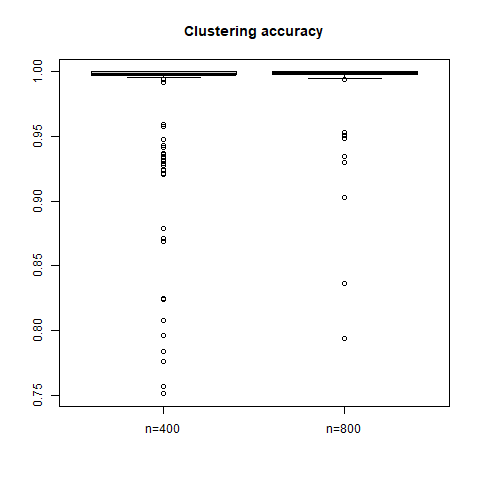
(a) Rand Index for the partitions obtained using the Cl-DRF estimator.

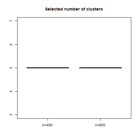
(b) Selected number of clusters.

Figure 13: Boxplot showing the clustering accuracy, computed with the Rand Index, over the $1000$ simulations. The Elbow method with the BIC criterion is used for selecting $C$. Simulated scenario with $C=5$.

The results in Figure 13 highlight that choose the correct number of clusters in all the $1000$ simulations. Therefore, the average Rand Index is again about unity, suggesting a very good cluster reconstruction properties of our Cl-DRF estimator. Therefore, Figure 13 highlights that the approach adopted for the number of clusters selection is appropriate even when the number of clusters is larger. Moreover, the Cl-DRF well reconstructs the ground truth if a correct number of clusters is specified.

We then evaluate the property of the Cl-DRF approach in estimating good DRFs from the policy perspective. The average DRF, for each of the $C=5$ clusters, in the case of $n=400$ are shown in Figure 14, while the case of $n=800$ is shown in Figure 15.

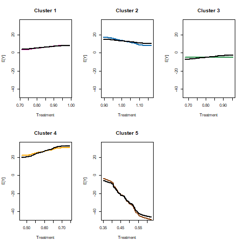
Figure 14: DRFs estimated using the Cl-DRF approach compared to the true simulated relationships. Simulated scenario I with $C=5$ and $n=400$.

Note: The colored lines represent the four simulated relationships for all values of treatment as in equation 18; the black lines are the estimated DRFs by using the Cl-DRF approach.

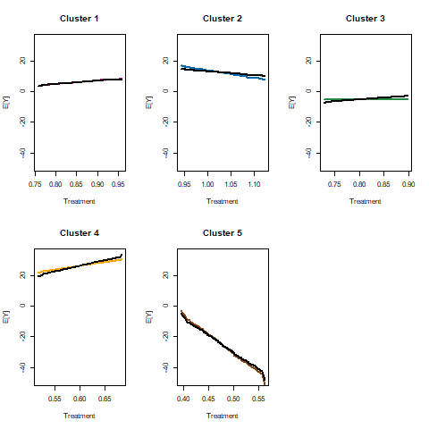
Figure 15: DRFs estimated using the Cl-DRF approach compared to the true simulated relationships. Simulated scenario I with $C=5$ and $n=800$.

Note: The colored lines represent the four simulated relationships for all values of treatment as in equation 18; the black lines are the estimated DRFs by using the Cl-DRF approach.

The figures highlight an important overlap between the colored lines, representing the true treatment-outcome relationships, and the black solid lines representing the ADRFs estimated with the Cl-DRF estimator. Therefore, we again get evidence of the usefulness of the Cl-DRF for policy purposes, since it allows a correct reconstruction of both the cluster structure and of the true ADRFs.

B.2 True number of clusters is C=3

For the case $C=3$ we consider the first three clusters adopted in the previous simulations, thus we refer to the previous two Sections for details on how the units have been simulated. Again, we compute the BIC criterion for different values of $C$ and choose the optimal number of clusters using the Elbow criterion. Figure 16 shows the boxplots of the clustering accuracy, computed with the Rand Index (Figure 16(a)), and of the selected number of clusters $C$ (Figure 16(b)) over the $1000$ simulations.

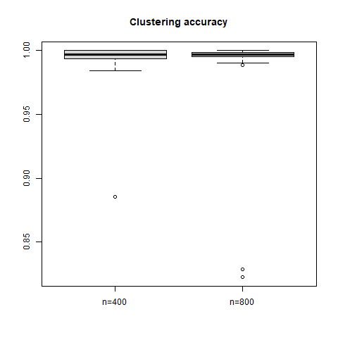
(a) Rand Index for the partitions obtained using the Cl-DRF estimator.

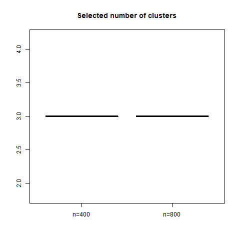
(b) Selected number of clusters.

Figure 16: Boxplot showing the clustering accuracy, computed with the Rand Index, over the $1000$ simulations. The Elbow method with the BIC criterion is used for selecting $C$. Simulated scenario with $C=3$.

The results in Figure 16 highlight that we again choose the correct number of clusters using the Elbow method. Interesitngly, the average Rand Index is again close to unity on average, so that we reconstruct the ground truth with the Cl-DRF estimator. The average DRF, for each of the $C=3$ clusters, in the case of $n=400$ are shown in Figure 17, while the case of $n=800$ is shown in Figure 18.

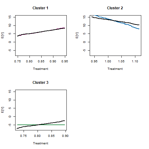
Figure 17: DRFs estimated using the Cl-DRF approach compared to the true simulated relationships. Simulated scenario I with $C=4$ and $n=400$.

Note: The colored lines represent the four simulated relationships for all values of treatment as in equation 15; the black lines are the estimated DRFs by using the Cl-DRF approach.

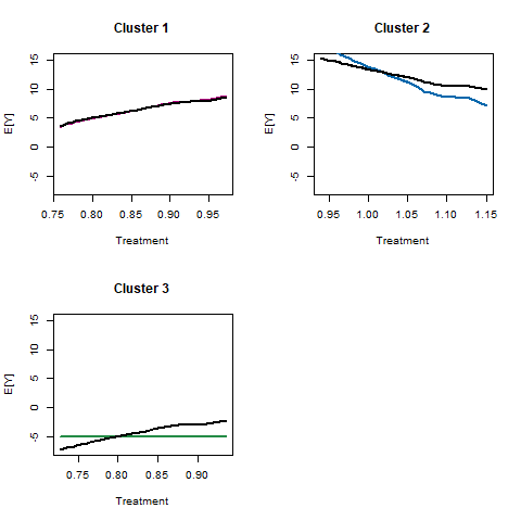
Figure 18: DRFs estimated using the Cl-DRF approach compared to the true simulated relationships. Simulated scenario I with $C=4$ and $n=800$.

Note: The colored lines represent the four simulated relationships for all values of treatment as in equation 15; the black lines are the estimated DRFs by using the Cl-DRF approach.

The results are in line with previous ones.

Appendix C Simulation results with random treatment

In what follows we show the results of simulation experiment considering random treatment. In particular, we assume that the treatment is not given by any covariate and $t_{i}\sim N(1,1)$ $\forall i=1,\dots,n$. Then, we simulate the outcome variable as a function of the simulated treatment according to the following within-cluster relationships

$$y_{i}=\begin{cases}\@add@centering\centering 5+t_{i}+e_{i}&\text{ for }c=1\\ 15-2t_{i}+e_{i}&\text{ for }c=2\\ -5-0.01t_{i}+e_{i}&\text{ for }c=3\\ 25+2t_{i}+e_{i}&\text{ for }c=4\\ -20-10t_{i}+e_{i}&\text{ for }c=5\\ \end{cases}$$ (19)

where $e_{i}\sim N(0,1)$, $\forall i$. We again consider three distinct simulation results, where $C=3$, $C=4$ and $C=5$. For the $C=5$ we consider all the relationships in Equation (19), while for $C=4$ and $C=3$ we consider the first four and the first three, respectively. We show the results of the comparison between true ADRF and those obtained with the proposed approach, assuming $n=800$, in Figures 19–21.

In sum, the results are in line with those discussed in Section 5. The approach adopted for selecting the number of clusters leads to very good performances and, under the correct selection of the number of clusters $C$, the Cl-DRF estimator reconstructs the clusters very well. The ADRFs estimated by the Cl-DRF estimator are also very close to the true ADRF, suggesting that the method is useful for policy purposes.

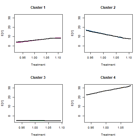
Figure 19: DRFs estimated using the Cl-DRF approach compared to the true simulated relationships. Simulated scenario with random treatment. $C=4$ and $n=800$.

Note: The colored lines represent the four simulated relationships for all values of treatment as in equation 15; the black lines are the estimated DRFs by using the Cl-DRF approach.

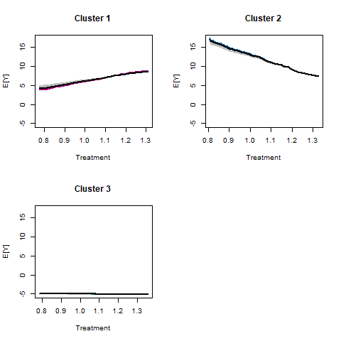
Figure 20: DRFs estimated using the Cl-DRF approach compared to the true simulated relationships. Simulated scenario with random treatment. $C=3$ and $n=800$.

Note: The colored lines represent the four simulated relationships for all values of treatment as in equation 15; the black lines are the estimated DRFs by using the Cl-DRF approach.

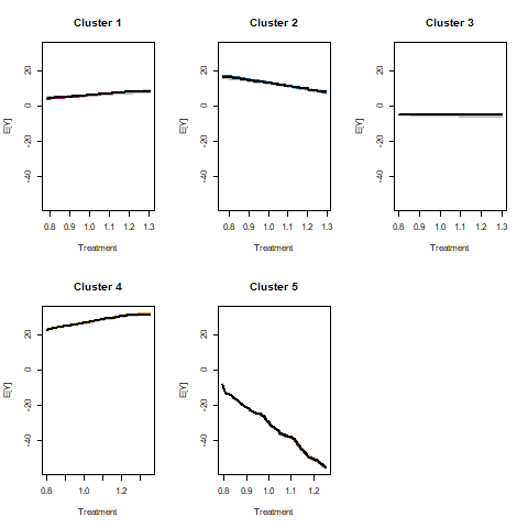
Figure 21: DRFs estimated using the Cl-DRF approach compared to the true simulated relationships. Simulated scenario with random treatment. $C=5$ and $n=800$.

Note: The colored lines represent the four simulated relationships for all values of treatment as in equation 15; the black lines are the estimated DRFs by using the Cl-DRF approach.

References

- Athey and Imbens, (2016) Athey, S. and Imbens, G. (2016). Recursive partitioning for heterogeneous causal effects. Proceedings of the National Academy of Sciences, 113(27):7353–7360.
- Athey and Imbens, (2017) Athey, S. and Imbens, G. W. (2017). The state of applied econometrics: Causality and policy evaluation. Journal of Economic perspectives, 31(2):3–32.
- Athey et al., (2019) Athey, S., Tibshirani, J., and Wager, S. (2019). Generalized random forests. The Annals of Statistics, 47(2):1148 – 1178.
- Austin, (2019) Austin, P. C. (2019). Assessing covariate balance when using the generalized propensity score with quantitative or continuous exposures. Statistical methods in medical research, 28(5):1365–1377.
- Becker et al., (2012) Becker, S. O., Egger, P. H., and Von Ehrlich, M. (2012). Too much of a good thing? on the growth effects of the eu’s regional policy. European Economic Review, 56(4):648–668.
- Becker et al., (2013) Becker, S. O., Egger, P. H., and Von Ehrlich, M. (2013). Absorptive capacity and the growth and investment effects of regional transfers: A regression discontinuity design with heterogeneous treatment effects. American Economic Journal: Economic Policy, 5(4):29–77.
- Bia and Mattei, (2012) Bia, M. and Mattei, A. (2012). Assessing the effect of the amount of financial aids to piedmont firms using the generalized propensity score. Statistical Methods & Applications, 21:485–516.
- Bonhomme and Manresa, (2015) Bonhomme, S. and Manresa, E. (2015). Grouped patterns of heterogeneity in panel data. Econometrica, 83(3):1147–1184.
- Branson et al., (2023) Branson, Z., Kennedy, E. H., Balakrishnan, S., and Wasserman, L. (2023). Causal effect estimation after propensity score trimming with continuous treatments. arXiv preprint arXiv:2309.00706.
- Callaway and Sant’Anna, (2021) Callaway, B. and Sant’Anna, P. H. (2021). Difference-in-differences with multiple time periods. Journal of econometrics, 225(2):200–230.
- Cerqua and Pellegrini, (2018) Cerqua, A. and Pellegrini, G. (2018). Are we spending too much to grow? the case of structural funds. Journal of Regional Science, 58(3):535–563.
- Cerqua and Pellegrini, (2023) Cerqua, A. and Pellegrini, G. (2023). I will survive! the impact of place-based policies when public transfers fade out. Regional Studies, 57(8):1605–1618.
- Cerqua and Pellegrini, (2024) Cerqua, A. and Pellegrini, G. (2024). Dove sta andando la valutazione delle politiche? In Valutazione delle politiche pubbliche. Che cosa abbiamo imparato? Donzelli Editore.
- Cox, (1958) Cox, D. R. (1958). Planning of experiments. .
- De Chaisemartin and d’Haultfoeuille, (2020) De Chaisemartin, C. and d’Haultfoeuille, X. (2020). Two-way fixed effects estimators with heterogeneous treatment effects. American Economic Review, 110(9):2964–2996.
- Dette and Neumeyer, (2001) Dette, H. and Neumeyer, N. (2001). Nonparametric analysis of covariance. the Annals of Statistics, 29(5):1361–1400.
- Fingleton et al., (2015) Fingleton, B., Garretsen, H., and Martin, R. (2015). Shocking aspects of monetary union: the vulnerability of regions in euroland. Journal of Economic Geography, 15(5):907–934.
- Fong et al., (2018) Fong, C., Hazlett, C., and Imai, K. (2018). Covariate balancing propensity score for a continuous treatment: Application to the efficacy of political advertisements. The Annals of Applied Statistics, 12(1):156–177.
- Hirano and Imbens, (2004) Hirano, K. and Imbens, G. W. (2004). The propensity score with continuous treatments. Applied Bayesian modeling and causal inference from incomplete-data perspectives, 226164:73–84.
- Huling et al., (2024) Huling, J. D., Greifer, N., and Chen, G. (2024). Independence weights for causal inference with continuous treatments. Journal of the American Statistical Association, 119(546):1657–1670.
- Imai and Van Dyk, (2004) Imai, K. and Van Dyk, D. A. (2004). Causal inference with general treatment regimes: Generalizing the propensity score. Journal of the American Statistical Association, 99(467):854–866.
- Li et al., (2018) Li, F., Morgan, K. L., and Zaslavsky, A. M. (2018). Balancing covariates via propensity score weighting. Journal of the American Statistical Association, 113(521):390–400.
- Morgado et al., (2023) Morgado, E., Martino, L., and San Millán-Castillo, R. (2023). Universal and automatic elbow detection for learning the effective number of components in model selection problems. Digital Signal Processing, 140:104103.
- Rand, (1971) Rand, W. M. (1971). Objective criteria for the evaluation of clustering methods. Journal of the American Statistical association, 66(336):846–850.
- Rodríguez-Pose and Garcilazo, (2015) Rodríguez-Pose, A. and Garcilazo, E. (2015). Quality of government and the returns of investment: Examining the impact of cohesion expenditure in european regions. Regional Studies, 49(8):1274–1290.
- Rubin, (1974) Rubin, D. B. (1974). Estimating causal effects of treatments in randomized and nonrandomized studies. Journal of educational Psychology, 66(5):688.
- Sugasawa, (2021) Sugasawa, S. (2021). Grouped heterogeneous mixture modeling for clustered data. Journal of the American Statistical Association, 116(534):999–1010.
- Tübbicke, (2021) Tübbicke, S. (2021). Entropy balancing for continuous treatments. Journal of Econometric Methods, 11(1):71–89.
- Tübbicke, (2023) Tübbicke, S. (2023). ebct: Using entropy balancing for continuous treatments to estimate dose–response functions and their derivatives. The Stata Journal, 23(3):709–729.
- Wager and Athey, (2018) Wager, S. and Athey, S. (2018). Estimation and inference of heterogeneous treatment effects using random forests. Journal of the American Statistical Association, 113(523):1228–1242.
- Wu et al., (2022) Wu, X., Mealli, F., Kioumourtzoglou, M.-A., Dominici, F., and Braun, D. (2022). Matching on generalized propensity scores with continuous exposures. Journal of the American Statistical Association, pages 1–29.
- Yiu and Su, (2018) Yiu, S. and Su, L. (2018). Covariate association eliminating weights: a unified weighting framework for causal effect estimation. Biometrika, 105(3):709–722.
- Zhao et al., (2008) Zhao, Q., Hautamaki, V., and Fränti, P. (2008). Knee point detection in bic for detecting the number of clusters. In International conference on advanced concepts for intelligent vision systems, pages 664–673. Springer.
- Zhao et al., (2020) Zhao, S., van Dyk, D. A., and Imai, K. (2020). Propensity score-based methods for causal inference in observational studies with non-binary treatments. Statistical methods in medical research, 29(3):709–727.