Converting sWeights to Probabilities with Density Ratios

Abstract

The use of machine learning approaches continues to have many benefits in experimental nuclear and particle physics. One common issue is generating training data which is sufficiently realistic to give reliable results. Here we advocate using real experimental data as the source of training data and demonstrate how one might subtract background contributions through the use of probabilistic weights which can be readily applied to training data. The sPlot formalism is a common tool used to isolate distributions from different sources. However, negative sWeights produced by the sPlot technique can lead to issues in training and poor predictive power. This article demonstrates how density ratio estimation can be applied to convert sWeights to event probabilities, which we call drWeights. The drWeights can then be applied to produce the distributions of interest and are consistent with direct use of the sWeights. This article will also show how decision trees are particular well suited to converting sWeights, with the benefit of fast prediction rates and adaptability to aspects of the experimental data such as data sample size and proportions of different event sources. We also show that a double density ratio approach where the initial drWeights are reweighted by an additional classifier gives substantially better results.

1 Introduction

A significant complication with creating training datasets for machine learning applications from experimental high energy and nuclear physics data is separating contributions from different event sources. For example, when considering a binary classification task aiming to separate signal events from backgrounds. In this case it is imperative that the training sample has reliable samples of the different distributions so that the machine learning algorithm can learn the underlying properties of both signal and background. One typical solution is to train the machine learning model on simulated data where the event sources can be trivially labelled. However this relies on excellent agreement between the simulation and real experiment on all training variables which is not always feasible and can lead to sub-optimal classification.

The sPlot [1] formalism aims to unfold the contributions of different event sources to the experimental data. The data is assumed to be characterised by discriminating variables for which the distribution of all sources of events are known, and control variables for which the distributions of some or all sources of events are unknown. These control variables are the features that would be used to train a machine learning model.

The sPlot technique is therefore an effective tool to separate various event sources, facilitating the creation of training samples from actual experimental data without the need for detector simulations. However, values of sWeights may be negative [1], which leads to complications when training machine learning algorithms. The weighted binary cross-entropy loss function is defined as:

$$L(f(x_{i}))=-\sum\limits_{i}w_{i}(y_{i}\text{log}f(x_{i})-(1-y_{i})\text{log}(1-f(x_{i})))$$ (1)

where $f(x_{i})$ is the output of a learning algorithm for event $i$ which has features $x_{i}$, weight $w_{i}$ and label $y_{i}$. In a binary classification task, $y_{i}$ is equal to either zero or one depending on which class the event belongs to, for example $y_{i}$ can be set to one (zero) for a signal (background) event. As learning algorithms are trained to minimise the loss, loss functions must have a lower bound of zero, otherwise the loss can then be made arbitrarily low. For example, given the loss in Equation 1 above, for a negatively weighted signal event where $y_{i}=1$ ($1-y_{i}=0$), the output of the learning algorithm could be made arbitrarily close to zero, which would make the loss for that event infinitely small. This is problematic, firstly because the signal event is assigned an output close to zero instead of close to one, and secondly because events with negative weights will then dominate the loss function. In general, loss functions that do not have a lower bound of zero will lead to issues during training and generally poor performance of the learning algorithm.

There has been some work in resampling negative weights for Monte Carlo event generators where negative weights are redistributed locally in phase space with any potential bias introduced by the resampling becoming arbitrarily small given sufficient statistics [2]. Although for Monte Carlo event generators it is always possible to generate larger datasets, experimental data may be statistically limited due to the availability and cost of data taking opportunities. As such, other approaches to resampling negative weights are desirable.

The use of machine learning to negate the impact of negative sWeights has previously been investigated for training learning models in classification tasks [3, 4]. This approach is akin to a regression problem where neural networks or Catboost decision trees [5] were trained to learn the signal and background probabilities produced by the sPlot technique using the mean square error loss function:

$$L(f(x_{i}))=\sum\limits_{i}(f(x_{i})-w_{i})^{2}\text{ .}$$ (2)

$x_{i}$ are the control variables over which the signal and background distributions were separated and the output of the neural network $f(x_{i})$ was constrained between zero and one by using an appropriate activation function in the output node such as a sigmoid function [3]. As such, the model will be able to predict weights between zero and one but will predict negative weights as zero and weights above one as one. When aiming to separate two classes, each contaminated by background events, the constrained weight $f(x_{i})$ was then used to replace the weight $w_{i}$ in the cross-entropy loss function described in Equation 1. This approach was shown to be useful in training algorithms to distinguish between the sWeighted signal and background sources [3, 4]. However the statistical properties associated with sWeights are then lost due to the loss being constrained to avoid negative weights and weights superior to one. For example, the sum of sWeights for a given event source must be equal to the yield for that event source. This requirement is unmet when constraining the weights between zero and one.

The key technique here is to recast the sWeights of a given event source to a probability of the event being from that source via the ratio of the density for that source divided by the sum of the densities of all sources. Binary classification can be used to estimate density ratios [6]. Previous works have investigated the use of probability classifier based density ratio estimation. Refs. [7, 8] used a neural network model to calculate weights used for reweighting Monte Carlo samples to more closely agree with data. Ref. [9] used a Boosted Decision Tree model with a bespoke objective function to iteratively reweight histograms. Refs. [10] and [11] used neural networks and boosted decision trees to model the detection efficiency and acceptance of high energy and nuclear physics experiments from simulations of the experiments.

In Ref. [12] a neural network was used to resample positive and negative weights produced by a Monte Carlo event generator using density ratio estimation. The neural network was trained to distinguish between two samples with features $x_{i}$ : one with weights given from the MC generator $w_{i}$ and the second with weights equal to 1. When considering the weighted binary cross entropy loss defined in Equation 1, $y_{i}\text{log}f(x_{i})$ goes to zero when $y_{i}=0$ and $(1-y_{i})\text{log}(1-f(x_{i}))$ goes to zero when $y_{i}=1$. As such, when the second sample with $y_{i}=0$ is weighted by 1, the weighted binary cross entropy loss can then be rewritten as:

$$L(f(x_{i}))=-\sum\limits_{i}(w_{i}y_{i}\text{log}f(x_{i})-(1-y_{i})\text{log}(1-f(x_{i})))\text{ .}$$ (3)

This loss function avoids issues due to negative weights encountered in Equation 1 so long as the sum of the weights from the MC event generator is less negative than the number of events produced by the event generator. That is to say that in the case where the sum of weights is negative, its absolute value must be smaller than the number of events produced by the event generator. Ref. [12] focused on resampling Monte Carlo weights, while pointing out this was applicable for any negative weights application. Here we specifically derive a similar approach to convert sWeights to probabilities, while the technique is again more general for the case of negative weight applications.

This article will demonstrate how sWeights can be transformed to event probabilities using density ratio estimation whilst preserving the sWeights’ statistical properties. In addition, this article will demonstrate how decision trees are ideally suited to learn sWeights. For certain applications, decision trees are preferable to neural networks as decision trees can have increased computational prediction rates whilst requiring almost no hyperparameter optimisation. Decision trees also typically don’t require as large training datasets as neural networks, which can be beneficial when the amount of experimental data is limited. It is therefore beneficial to have flexibility in the choice of learning algorithm.

The rest of the article is organised as follows: Section 2 will review the sPlot formalism before describing how decision trees cope with negative weights. The remainder of Section 2 will describe how density ratios can be used to convert sWeights to probabilities. Section 3 will then use two case studies, one based on a toy dataset and one based on experimental data taken with the CLAS12 experiment [13], to demonstrate the method’s good performance. Section 4 will end the article with brief conclusions and outlook.

2 Methodology

2.1 Summary of sPlot

The sPlot [1] technique allows one to disentangle event distributions of different species from a data sample via a discriminatory variable, in which the different species have different distributions of known type. A common use case is to remove background to leave a signal only distribution. This is its purpose in this work where we wish to train classifiers on signal distributions from real experimental data. Essentially, sPlot generalises side-band subtraction weights to situations where there is no clear region of isolated background which can be used to subtract from the total event sample. Similar to side-bands it requires that the discriminatory variable and variables of interest are independent of each other. A further generalisation of sPlot to treat cases where variable dependence arises is suggested in Custom Orthogonal Weight functions for Event Classification [14]. This work also provided the implementation of sWeights used here [15].

The sPlot technique allows to reconstruct variables’ of interest distributions for each event source using the probability density functions (pdf) of each, often established by fitting the expected pdfs on the discriminating variables. In effect, the behavior of the individual sources of events with respect to the variables of interest is inferred from the knowledge available for the discriminating variables by assigning an sWeights to each event in the data sample.

One essential characteristic of sWeights is that weights used to remove background species tend to be negative. On one hand this allows the statistical properties of the disentangled data-set to be robust, i.e. uncertainties can be reliably determined from sWeights subtracted data provided these weights are propagated to the uncertainties appropriately [16]. On the other hand this provides issues for machine learning applications as described in the introduction.

2.1.1 Decision Trees

For our probabilistic classification task we chose to test a selection of Decision Trees as these naturally accept negative sample weights, such as sWeights, when trained with the binary cross entropy loss function of Equation 3. Decision trees are composed of nodes which branch out into child nodes. The last node at the end of a branch is known as a leaf and returns a prediction, which in a classification task should be one of the classes in the training data. Decision trees attempt to classify the training data by repeatedly splitting the training data into the left and right child nodes. The splits are performed by applying simple requirements on a random choice of input features such that a specified loss function is minimised. The splitting continues until either all leaves contain one event each or a specified maximum depth is reached. The prediction rate of decision trees can be increased by discretising the input feature space, allowing the decision tree to operate on a bin value rather than specific values of the input features. This type of decision tree is called a histogram decision tree.

One common issue with decision trees is that they are prone to overfitting the training data. One simple solution to reduce overfitting and generally improve the performance of decision trees is so called boosting. The idea behind boosting is that it is generally easier to train several smaller models than a single large model whilst still avoiding over-fitting. Popular boosting algorithms include adaptive boosting [17] or gradient boosting [18]. The boosting algorithm employs multiple decision trees trained one after the other, with subsequent decision trees focused on events incorrectly classified by previous decision trees by assigning a weight to such events. A user defined maximum number of decision trees or a threshold on the training error will stop the boosting process.

The default node splitting loss in the scikit-learn [19] implementation of gradient boosted decision trees is the weighted binary cross-entropy loss. The loss function can be made to avoid issues in training due to negative sWeights by creating a training sample with one class weighted with sWeights and the other with weights set to 1 as defined in Equation 3 and explained in the introduction. The output of a decision tree differs from neural networks in that the output of a leaf depends on the proportion of a class $k$ in a leaf $m$ [20]. For an unweighted classification task, the output is given by:

$$p_{mk}=\frac{N_{mk}}{N_{m}}$$ (4)

where $N_{m}$ is the number of events in leaf $m$ and $N_{mk}$ is the number of events in leaf $m$ belonging to class $k$. For a binary classification task with two classes, the ratio between the proportion of both classes $p_{m1}$ and $p_{m2}$ determines the prediction decision. If $\frac{p_{m1}}{p_{m2}}>1$, then the prediction for events that reach this leaf will be that they belong to class 1.

For a weighted binary classification task, the sample weight for the first class is $S^{+}_{1}-S^{-}_{1}$, the difference between the sum of the positive weights $S^{+}_{1}$ and the sum of the absolute value of negative weights $S^{-}_{1}$. If the sample weight for the second class is $S_{2}$, the proportion of each class in a node will be:

$$p_{1}=\frac{S^{+}_{1}-S^{-}_{1}}{N}\text{ and }p_{2}=\frac{S_{2}}{N}$$ (5)

where the subscript $m$ was dropped for simplicity. The ratio $p_{1}/p_{2}$ from Equation 5 is unchanged when removing negatively weighted events from the first class and adding positively weighted samples to the second class with weights $S^{+}_{2}$ such that:

$$\frac{S^{+}_{1}-S^{-}_{1}}{S_{2}} =\frac{S^{+}_{1}}{S_{2}+S^{+}_{2}}$$ (6)

$$\Rightarrow S^{+}_{2} =\frac{S_{2}S^{-}_{1}}{S^{+}_{1}-S^{-}_{1}}\text{ .}$$ (7)

In short, negative weights can be used to train scikit-learn decision trees with the right loss function as negative weights in a given sample are, in effect, akin to adding positively weighted events to the other sample.

2.2 Learning Weights using Density Ratios

The aim of the sPlot formalism is to unfold the true distribution of one or more control variables $x_{i}$ for events of different sources using the knowledge available from discriminating variables on the distribution of these sources. The source are classed in species (e.g. signal and background). The sPlot technique provides a consistent representation of how all events from the species are distributed in $x_{i}$ [1]. Summing the sWeights for a given species then recovers the yield of that species obtained by a fit to the discriminating variable. For example, by summing the signal weights one recovers the signal yield. Summing the weights for all species allows to recover the entire data distribution composed of the different species.

The sWeights for a given species can then be taken as the ratio of the probability density for that species over the sum of probability densities of all species in the data $D_{all}(x_{i})$. For a distribution separated into signal and background species with probability densities $D_{S}(x_{i})$ and $D_{B}(x_{i})$ respectively, the density ratio weights drWeights $W_{dr}(x_{i})$ distribution over control variables $x_{i}$ is written as the density ratio:

$$W_{dr}(x_{i})=\frac{D_{S}(x_{i})}{D_{S}(x_{i})+D_{B}(x_{i})}=\frac{D_{S}(x_{i})}{D_{all}(x_{i})}\text{ .}$$ (8)

The knowledge of this ratio is sufficient to model the signal sWeights distribution. Note that this ratio would also be preserved in the presence of more than one background species, as the distribution of all events will simply be expanded to a sum of the signal distribution and all background species’ contribution: $D_{all}(x_{i})=D_{S}(x_{i})+D_{B1}(x_{i})+D_{B2}(x_{i})...$ A convenient technique for density ratio estimation is to treat it as a binary classification problem. Similarly to the neural resampler of Ref. [12], a machine learning model can be trained on data separated into two classes: the first with density distribution $D_{S}(x_{i})$ consisting of all events in the data weighted with the signal sWeights. The second with density distribution $D_{all}(x_{i})$ consisting of all events uniformly weighted with weights set to one. $D_{S}(x_{i})$ is labelled class 1 and $D_{all}(x_{i})$ is labelled class 0. The output of the classifier $f(x_{i})$ for class 1 is then:

$$f(x_{i}) =\frac{D_{S}(x_{i})}{D_{S}(x_{i})+D_{all}(x_{i})}=\frac{D_{S}(x_{i})}{D_{S}(x_{i})+D_{S}(x_{i})+D_{B}(x_{i})}$$

$$\Rightarrow\frac{1}{f(x_{i})} =\frac{D_{S}(x_{i})}{D_{S}(x_{i})}+\frac{D_{S}(x_{i})}{D_{S}(x_{i})}+\frac{D_{B}(x_{i})}{D_{S}(x_{i})}$$

$$\Rightarrow\frac{1}{f(x_{i})}-1 =\frac{1-f(x_{i})}{f(x_{i})}=\frac{D_{S}(x_{i})+D_{B}(x_{i})}{D_{S}(x_{i})}$$

$$\Rightarrow W_{dr}(x_{i}) =\frac{f(x_{i})}{1-f(x_{i})}\text{ .}$$ (9)

Overall, the two key aspects of converting sWeights to probabilities using density ratio estimation are first that creating the training sample with one class weighted by the sWeights and the other with weights set to one allows to use the binary cross-entropy loss function without issues in training due to negative sWeights as it preserves a lower bound of zero in the loss function. Second, creating the training sample in such a way allows a binary classification model to learn the ratio of the signal probability density divided by the sum of the probability densities of all species, which is equal to the signal sWeights distribution. Binary classification for density ratio estimation is therefore perfectly suited to convert sWeights to probabilities. Note that the learning algorithm should only be trained with the control variables as inputs, and the learned model works only at the distribution level and not on an event by event basis.

Section 2.1.1 demonstrated how the scitkit-learn implementation of boosted decision trees allows for training with negative weights. In the schema proposed above, negative weights in class 1, with density distribution $D_{S}$, would have the same effect as adding positive weights to class 0, with density distribution $D_{all}$. The density ratio which describes the drWeights $W_{dr}$ is preserved by boosted decision trees, as removing negative weights from $D_{S}$ and adding the corresponding positive weights to $D_{all}$ must preserve the overall ratio.

A final consideration is preserving the uncertainty associated with using the sWeights. This uncertainty is calculated largely by taking the sum of the squared sWeights. However, Ref. [12] showed that calculating the uncertainty as the sum of the resampled weights squared gives incorrect uncertainties. There are two possible solutions, first to just use the sWeights for the uncertainty calculation. Second, Ref. [12] also showed that the uncertainty itself can be converted using density ratio estimation which preserves the uncertainty. For the remainder of this article, we choose the first option, to carry over the uncertainty from the sWeights, but it is important to note that the uncertainty on the sWeights can also be learned.

3 Case Studies

3.1 Toy Example

This section will present a toy example to illustrate the performance of the density ratio estimation of sWeights. In the toy example, a simple event generator produces three dimensional events where the first variable is akin to a mass such as the invariant mass of a given reaction, the second variable is akin to an azimuthal ($\phi$) angular distribution and the third variable is $z=\cos{\theta}$. Signal events were generated with a Gaussian distribution in mass and a $\cos{2\phi}$ asymmetry of amplitude 0.8. Background events were generated with a Chebyshev polynomial distribution in mass and a $\cos{2\phi}$ asymmetry of amplitude -0.2. The ratio of signal to background was varied in different tests. The mass variable was used as the discriminatory variable, allowing to separate the signal and background distributions via the weights. The aim of this toy example was then to measure the signal asymmetry in $\phi$ by unfolding the signal and background distributions in the control variables $\phi$ and $z$.

The generated mass distribution was fitted using the sum of the signal and background pdfs used to generate the events with the mean, sigma and polynomial coefficients allowed to vary in the fit. The fit was then used to calculate the signal and background sWeights using the implementation from Ref.[14, 15]. Figure 1 shows a comparison of the mass, $\phi$ and Z distributions for all events and these same events with signal and background sWeights applied, with a signal to background ratio of 1:2. As can be seen, the sum of the signal and background weights allows to reproduced the total distribution. The discriminatory variable, mass, contains negative bins for the signal and background distribution where these events are effectively subtracted to give the disentangled control distributions.

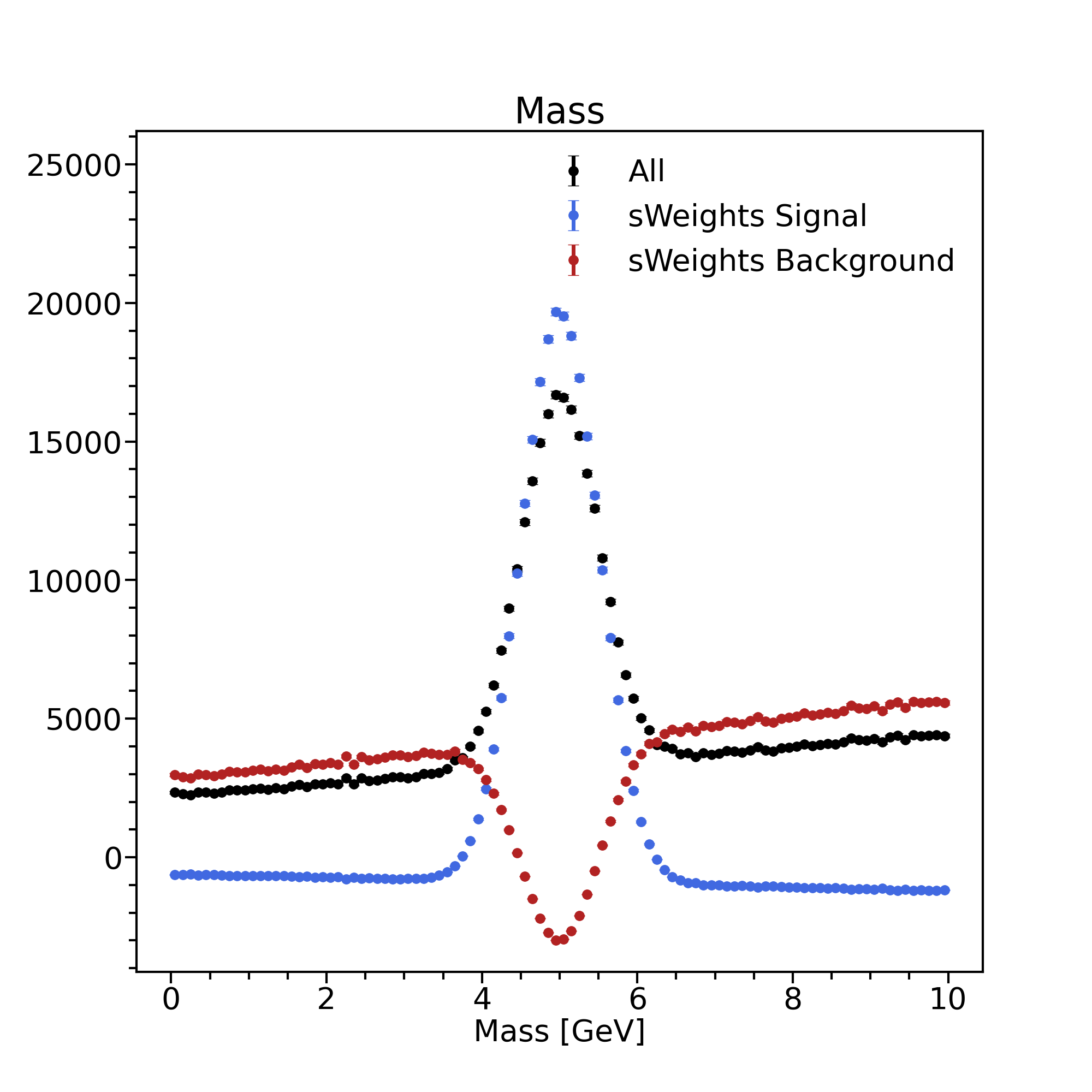
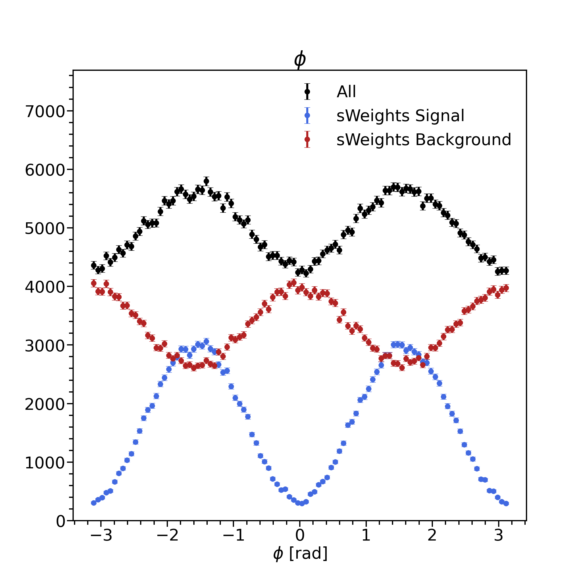
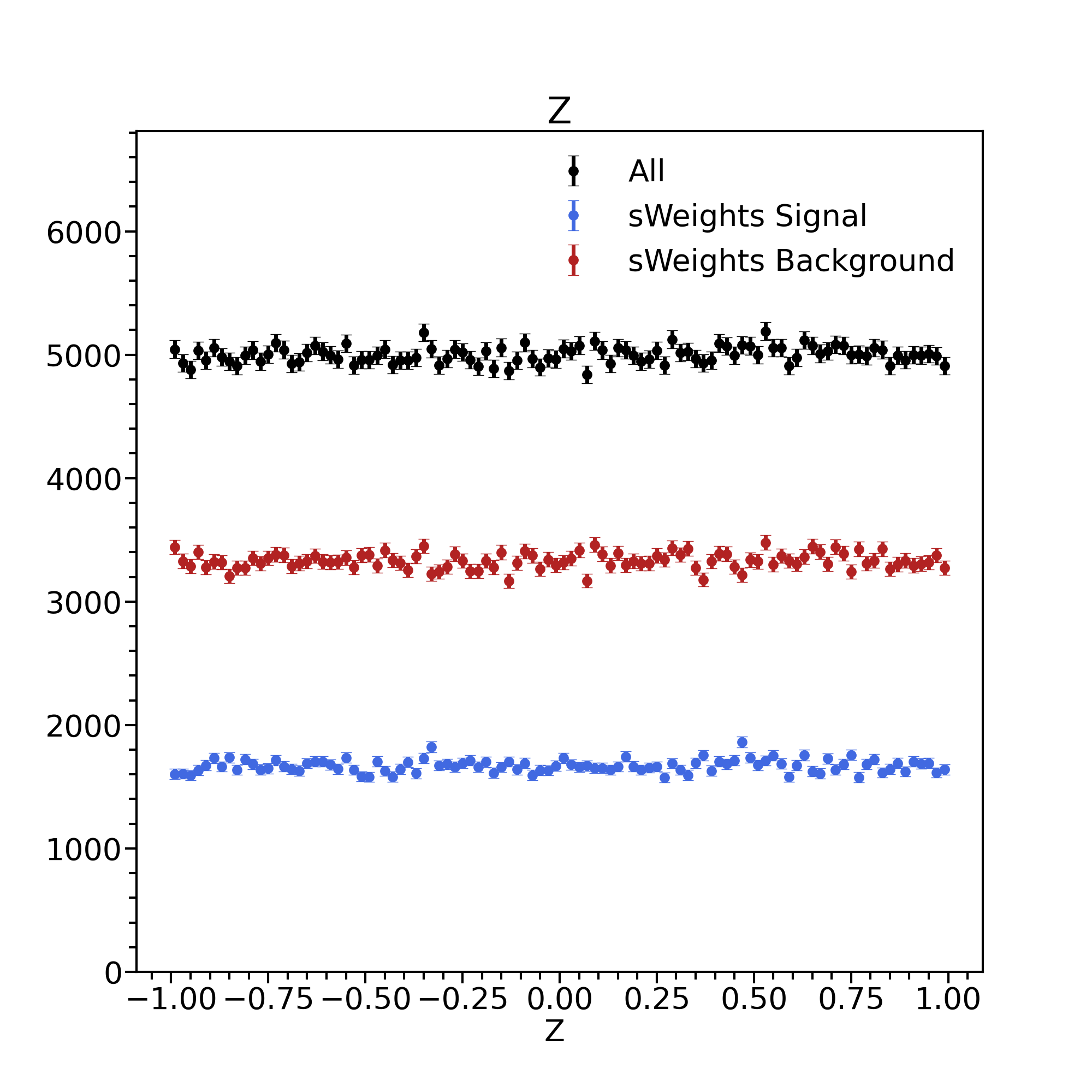
Figure 1: The total (black) distribution in mass (left), $\phi$ (middle) and Z (right) compared to the same distribution with signal or background sWeights applied.

The methodology described in Section 2 was then applied to convert the sWeights using density ratio estimation. The scikit-learn library [19] was used to test both a gradient boosted decision tree (GBDT) and a histogram gradient boosted decision tree (HistGBDT). Both the GBDT and HistGBDT were given a maximum depth of 10 and otherwise default parameters. The neural resampling method described in Ref. [12] was also applied to the toy example. Ref. [12] used particle flow networks (PFN) [21] based on the deep sets architecture [22]. PFNs are general models designed for learning from collider events as unordered, variable-length sets of particles rendering them unsuited to this application with only two variables. Instead neural networks with 7 hidden layers and 1024, 512, 256, 128, 64, 32, 16 nodes respectively were implemented using tensorflow [23]. The hidden layers all had RELU activation functions, with the output layer having a sigmoid activation function, and the network was trained with an ADAM optimiser [24] for 50 epochs. Ref. [11] found that a second iteration of the density ratio estimation, essentially using density ratio estimation for a reweighting step, improved the performance by fine tuning the model. This was also tested here. This second iteration weighted the class labelled 0 with the weights produced by the first density ratio estimation, the predicted weights were then taken as the product of the weights obtained by both individual models.

Training and prediction times were estimated using 5 cores of a AMD EPYC 9554 64-Core Processor at 3.1 GHz. $3.5\times 10^{5}$ events were generated, which leads to a training sample with $7\times 10^{6}$ events as the same events are found in both class 1 and class 0, albeit with and without sWeights weighting. The GBDTs train at a rate of 4kHz and had a prediction rate of roughly 1.6 MHz. The HistGBDTs had a training rate of roughly 1 MHz, with a prediction rate of roughly 20 MHz. The neural network described above had a training rate of 2 kHz with a prediction rate of 0.5 MHz.

The $\phi$ asymmetry was then extracted via the weighted datasets. To do this a 1D histogram was generated in $\phi$ with 100 bins, each bin filled with the relevant signal sWeights or converted weights called drWeights. While the drWeights reproduced the correct distribution, the uncertainties were calculated from the sum of the original sWeights in each bin to allow correct propagation of errors to the fit result as discussed at the end of Section 2.2. Fits were performed by minimizing the $\chi^{2}$ between the model and the binned histogram using the iminuit package [25].

If the sWeights and drWeights accurately separate the signal and background distributions in $\phi$ then the asymmetry obtained by the fit should be consistent with the generated value of 0.8. Several different convertor models were tested along with a double density ratio estimation where the first model was fine tuned by the second model. The total number of generated events was $10^{5}$ with a signal to background ratio of either 1:2 or 1:9. All events were used in training. The entire chain of generating data, fitting and calculating sWeights, training the density ratio model and measuring the $\phi$ asymmetry was repeated 50 times to allow us to determine the robustness of the conversion procedure. Table 1 reports the mean amplitude and uncertainty reported from by the 50 iminuit fits and the standard deviation of the amplitude over the 50 datasets. The expectation is that the mean should be consistent with the nominal value of 0.8, while the mean uncertainty and standard deviation should be numerically similar i.e. the fluctuation of results is consistent with the calculated uncertainty. The first row shows the results for the sWeighted distributions that we are trying to emulate.

	Mean	$\sigma$	Uncertainty	$\frac{\sigma}{\text{Uncertainty}}$	Mean	$\sigma$	Uncertainty	$\frac{\sigma}{\text{Uncertainty}}$
Signal:Background	1:2	1:2	1:2	1:2	1:9	1:9	1:9	1:9
sWeights	0.802	0.0082	0.0089	0.92	0.804	0.0244	0.0274	0.89
GBDT	0.796	0.0094	0.0091	1.03	0.707	0.0779	0.0271	2.87
GBDT & GBDT	0.807	0.0093	0.0092	1.01	0.793	0.0260	0.0285	0.91
GBDT & HistGBDT	0.810	0.011	0.0092	1.20	0.791	0.0347	0.0283	1.23
HistGBDT	0.760	0.0169	0.0089	1.90	0.643	0.0356	0.0261	1.36
HistGBDT & GBDT	0.788	0.0115	0.0091	1.26	0.739	0.0326	0.0281	1.16
HistGBDT & HistGBDT	0.782	0.0112	0.0090	1.24	0.713	0.0342	0.0274	1.25
NN	0.782	0.0262	0.0089	2.94	0.743	0.0417	0.0264	1.58
NN & GBDT	0.822	0.0130	0.0093	1.40	0.826	0.0369	0.0299	1.23
NN & HistGBDT	0.813	0.0180	0.0093	1.94	0.816	0.0351	0.0291	1.21

Table 1: Comparison of the $\phi$ asymmetry measured for various models used by the density ratio estimation. The signal distribution was generated with a $\phi$ asymmetry of 0.8 for $10^{5}$ events with a signal to background ratio of 1:2 or a signal to background ratio of 1:9. The data generation and training were repeated 50 times. The mean and standard deviation ($\sigma$) of the measured asymmetries are reported, along with the mean uncertainty.

We observe from the results in Table 1 that all convertors except the HistGBDT perform adequately in reproducing the amplitude (mean value) for the 1:2 signal to background case. In particular models with a double density ratio, or reweighting step, are an improvement on the single step case. For the 1:9 case where the background dominates, models with the GBDT reweighting step perform well, while the others do not give as accurate an amplitude. In all cases the uncertainty is consistent as it is just a property of the data statistics and we are using the sWeighted sum of the weights squared. The standard deviation however does vary significantly from the given uncertainty showing a lack of robustness in the procedure for some convertor models. This is likely due to some random events getting inaccurate weights and thereby less accurate $\phi$ distributions. This also seems to be more of an issue for the neural network based models and in the higher background tests. On the other hand the double GBDT model seems to perform admirably even with 1:9 signal to background and would seem to be the most robust convertor.

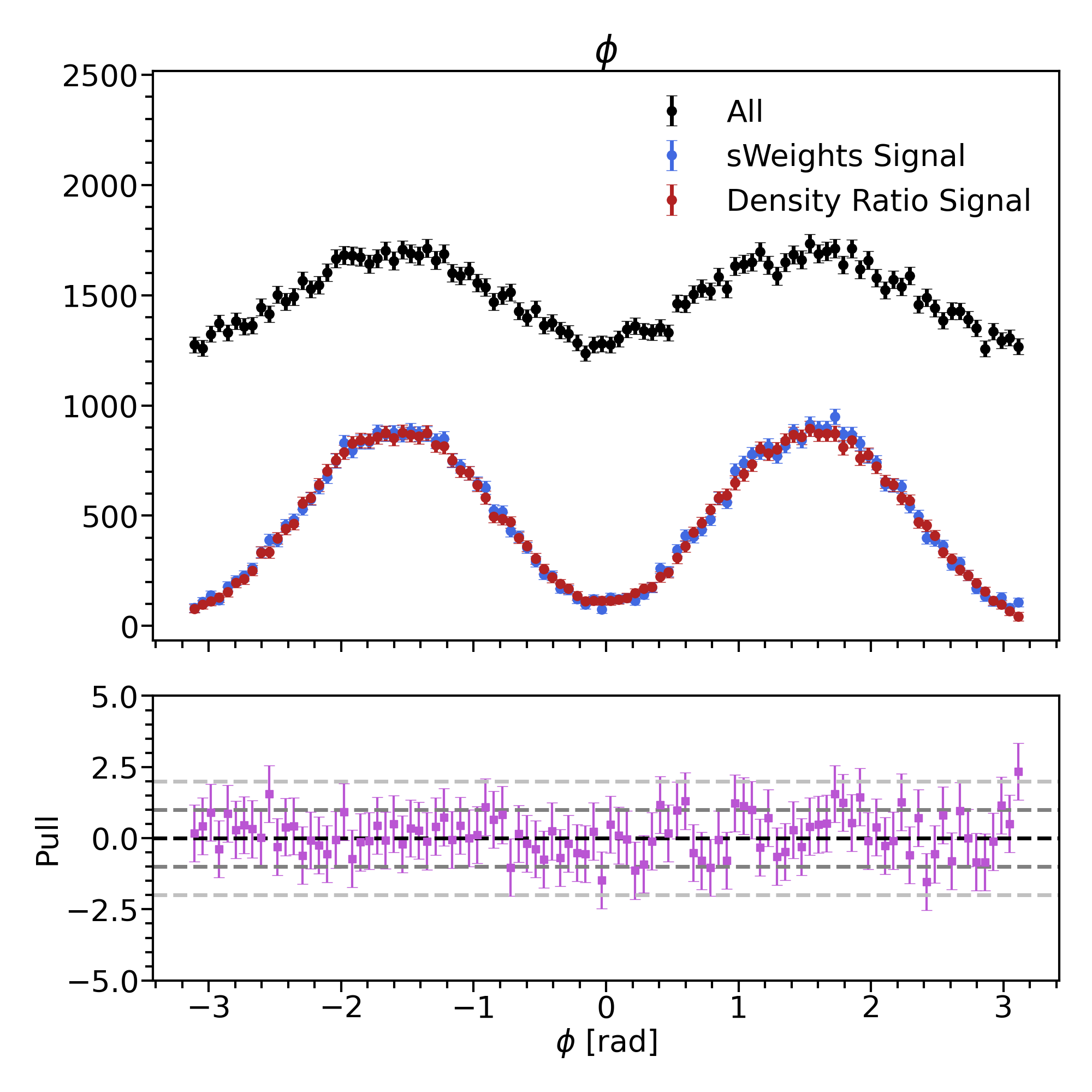
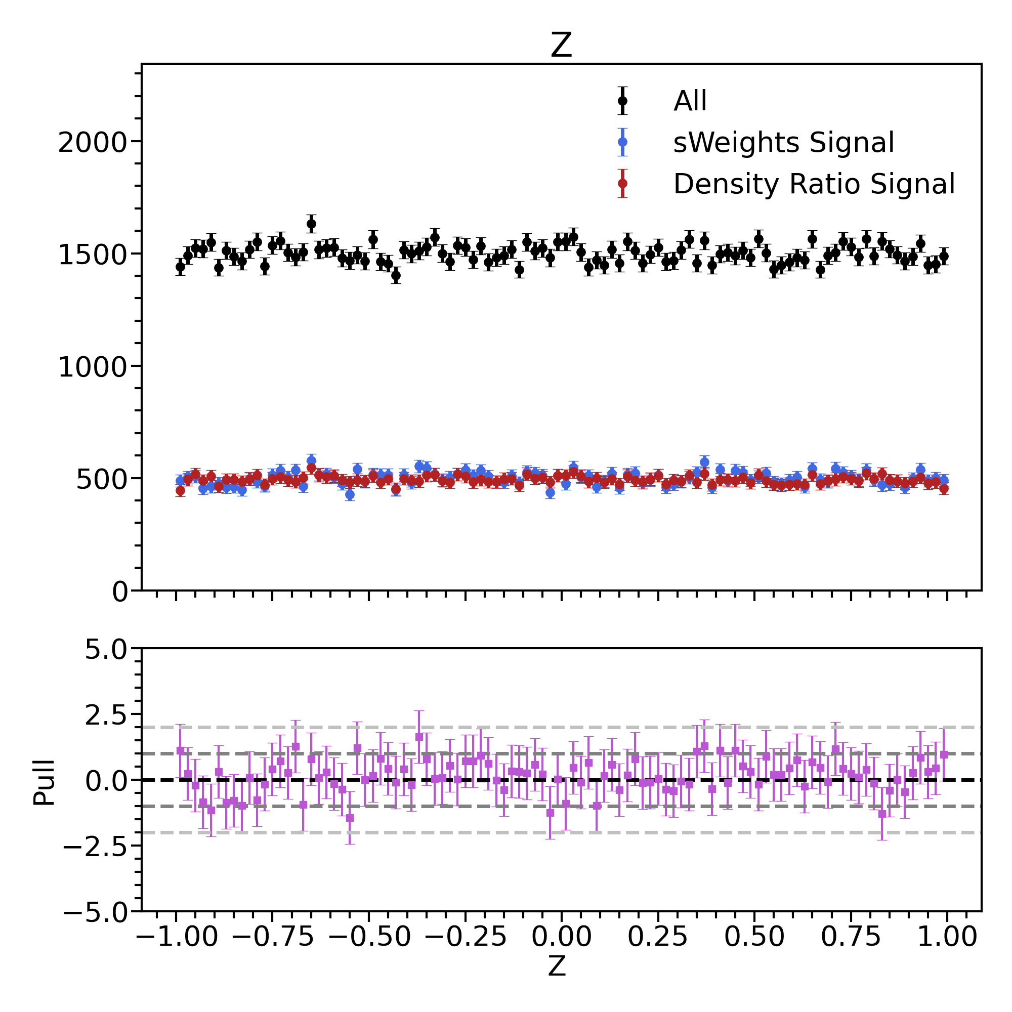
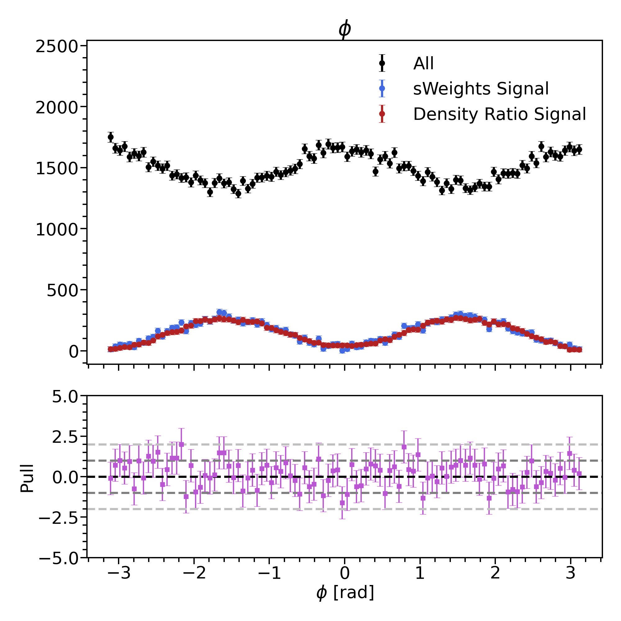
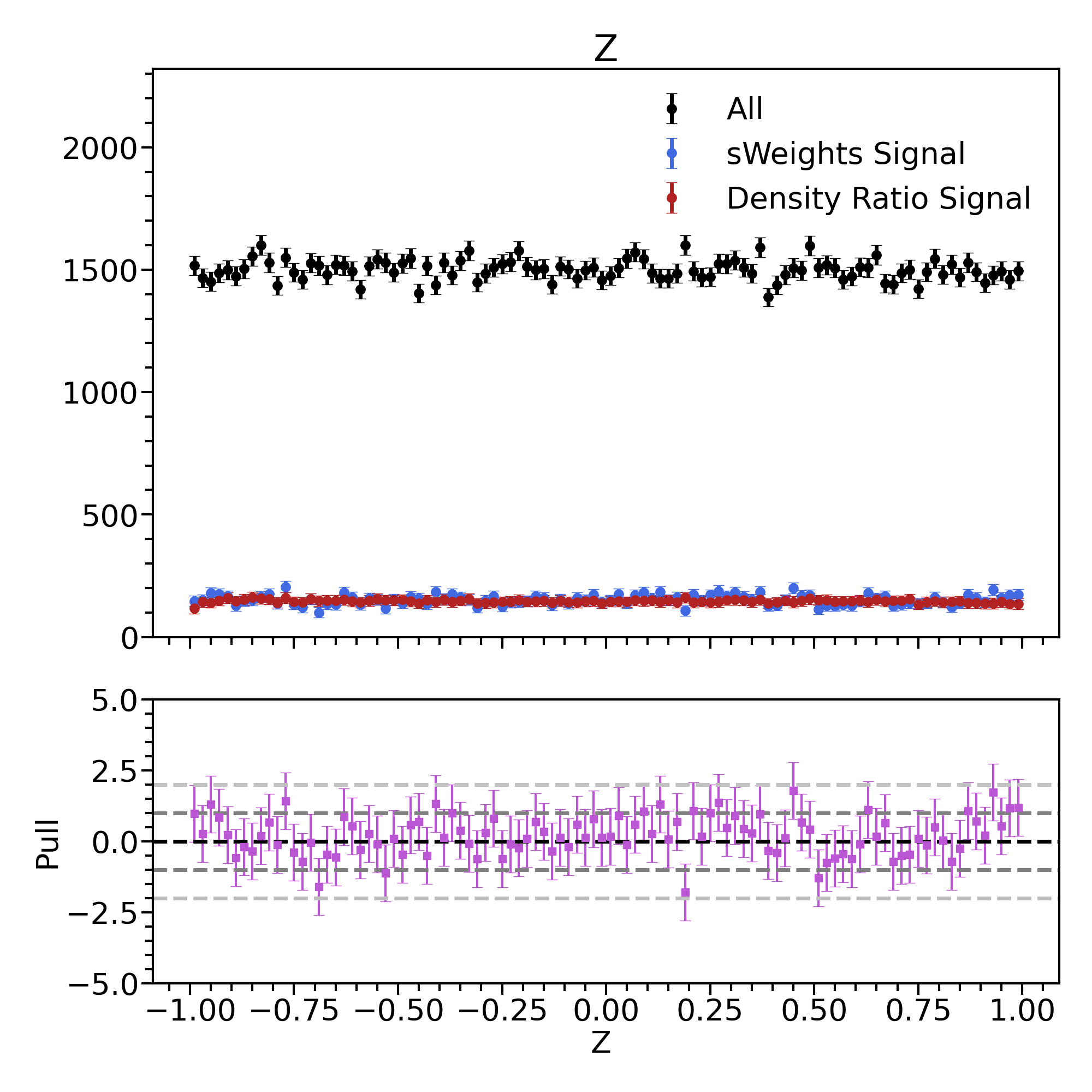
Figure 2: The total (black) distribution in $\phi$ (left) and Z (right) compared to the same distribution with signal sWeights applied (blue) or the drWeights applied (red). The top row was generated with a signal to background ratio of 1:2, wereas the bottom row has a signal to background ratio of 1:9. The pull between the sWeights and drWeights distributions is also shown below all distributions. The drWeights are estimated using the GBDT and GBDT double density ratio.

Figure 2 shows a comparison of the signal distributions unfolded in $\phi$ and $z$ using the signal sWeights and drWeights for the best algorithm, namely the double density ratio using the GBDT followed by another GBDT. Figure 2 also compares the case where the events were generated with a signal to background ratio of 1:2 or 1:9. A total of 0.5M events were generated events where 0.35M were used in training and 0.15M were used for testing and are plotted in Figure 2. The uncertainties are calculated from the original sWeights. Figure 2 also shows the bin-by-bin pull distributions defined as the difference between the bin values for the two distributions divided by the sum squared of their uncertainties. Overall the density ratio estimation is able to accurately reproduce the $\phi$ and Z signal weighted distributions as shown by the pulls which are largely consistent with being less than 1. This also holds in the case of a dominant background as shown in the bottom row of Figure 2. For both signal to background ratios of 1:2 or 1:9, the $\phi$ asymmetries measured with the signal drWeights were consistent within uncertainties with the generated value of 0.8.

The number of generated events was then varied to ascertain the impact this has on the density ratio estimation using the preferred GBDT and GBDT double density ratio. The results are shown in Table 2, together with the results from the sWeights fitting. The asymmetry amplitude was again generated at 0.8, and here the signal to background ratio was fixed to the large background case at 1:9. In all cases, even with as few as $10^{3}$ generated events, the asymmetry measured with the drWeights is consistent with the generated asymmetry of 0.8. The mean standard deviation and uncertainty on the asymmetry are generally consistent. At 1000 events, corresponding to 100 actual signal events, the fit error is twice the size of the standard deviation, suggesting the uncertainty is overestimated by a factor 2. This is not surprising given that the sum of the squared weights contribution to the uncertainty is less valid at low statistics. Also at 1000 events the drWeights clearly outperform the sWeights. This is due to the latter producing bins with unphysical negative counts, a problem which is resolved by using probability weights. This issue is ultimately an artifact of the weighted binned fitting, which is not the ideal method for extracting parameters from data. Instead one should use an event-by-event maximum likelihood procedure to produce reliable results, but this is outwith the scope of this work. The good performance of the drWeights even with large backgrounds and small event samples is a key consideration, given that experimental datasets may be limited and may have irreducible backgrounds. Although it is worth noting that drWeights should only be used when positive definite probabilities are required as the sWeights proved to be more generally more reliable, overall the drWeights were found to be a robust conversion of sWeights to probabilities.

Number of	sWeights	sWeights	sWeights	sWeights	drWeights	drWeights	drWeights	drWeights
Events	Mean	$\sigma$	Uncertainty	$\frac{\sigma}{\text{Uncertainty}}$	Mean	$\sigma$	Uncertainty	$\frac{\sigma}{\text{Uncertainty}}$
$10^{3}$	17.94	84.81	14.67	5.78	0.679	0.2710	0.5902	0.46
$10^{4}$	0.870	0.1090	0.0953	1.14	0.778	0.0929	0.1038	0.89
$10^{5}$	0.804	0.0244	0.0274	0.89	0.793	0.0260	0.0285	0.91
$10^{6}$	0.799	0.0104	0.0090	1.16	0.792	0.0110	0.0092	1.20

Table 2: Comparison of the $\phi$ asymmetry measured on the sWeights signal distribution and the drWeights (DR) signal distribution when increasing the number of generated events. The signal distribution was generated with a $\phi$ asymmetry of 0.8 and a signal to background ratio of 1 to 9. The data generation and training were repeated 50 times. The mean and standard deviation ($\sigma$) of the measured asymmetries are reported, along with the mean uncertainty. The drWeights are estimated using the GBDT and GBDT double density ratio. Note that to extract the $\phi$ asymmetry, $\phi$ was binned in 100 bins for all tests except at $10^{3}$ events where $\phi$ was binned in 50 bins due to lower statistics.

The toy example presented in this section is contained in the Github repository found at [26]. A generator class produces the total distribution composed of the signal and background distributions, calculates the signal and background sWeights and fits the $\phi$ asymmetry. A plotter class allows to produce the plots shown in this section. A performance class allows to run the tests described here. A trainer class allows to train the models as described in this article. A training script then allows to train the decision tree based models and the neural resampler. The toy example can be used as example of how to train and deploy the methods described in Section 2 and in Ref. [12].

3.2 $ep\to e^{\prime}\pi^{+}n$ in CLAS12

This section will demonstrate an application of the method presented in Section 2 to experimental nuclear physics data. The Continuous Electron Beam Accelerator Facility (CEBAF) [27] delivers an electron beam with energy up to 12 GeV to the four experimental halls at the Thomas Jefferson National Accelerator Facility (JLab). The CEBAF Large Acceptance Spectrometer at 12 GeV (CLAS12) [13] is located in Hall B. The CLAS12 experimental program broadly encompasses electroproduction experiments aiming to further the global understanding of hadronic structure and Quantum Chromodynamics [28]. The CLAS12 detector was built to have full azimuthal angular coverage and a large acceptance in polar angle, allowing measurements to be made over large kinematic ranges [13]. Very low polar angular coverage, from 2.5 to 5 degrees, is enabled by the forward tagger (FT), whilst the forward detector (FD) covers the range of polar angles from 5 to 35 degrees and is segmented into six sectors of azimuthal angle. The central detector (CD) covers the polar angular range of 35 to 125 degrees.

The Forward Electromagnetic Calorimeters (ECAL) [29] are employed to detect and identify neutrons in the FD. Studies of neutron detection in the FD, for example measuring the neutron detection efficiency or establishing corrections to the measured neutron momenta, often employ the exclusive reaction $ep\to e^{\prime}\pi^{+}n$. A neutron reconstructed from the reaction $ep\to e^{\prime}\pi^{+}X$ is compared to the detected neutron, allowing estimates of quantities like the neutron detection efficiency. Several analysis procedures are made to check that the detected neutron corresponds to the reconstructed neutron, such as restricting the direction of the reconstructed neutron to the fiducial region of the FD and requiring that the reconstructed and detected neutron have a small difference in polar and azimuthal angles.

In this analysis the mass of the missing particles in the reaction $ep\to e^{\prime}\pi^{+}X$ close to the neutron mass was fitted to estimate the number of signal events where the exclusive reaction $ep\to e^{\prime}\pi^{+}n$ was produced. Figure 3 shows the fit of the missing mass of $ep\to e^{\prime}\pi^{+}X$ with the background described by a third order Chebyshev polynomial. The neutron signal was given by a template histogram from simulated data that was created by generating events for the reaction $ep\to e^{\prime}\pi^{+}n$ and running them through the CLAS12 simulation framework, GEMC [30]. This fit allowed sWeights to be assigned to separate the neutron signal from the underlying background. We are now able to disentangle neutron and background distributions. However if we wish to train a machine learning algorithm with these signal neutrons we should convert the sWeights to drWeights as described in Section 2.

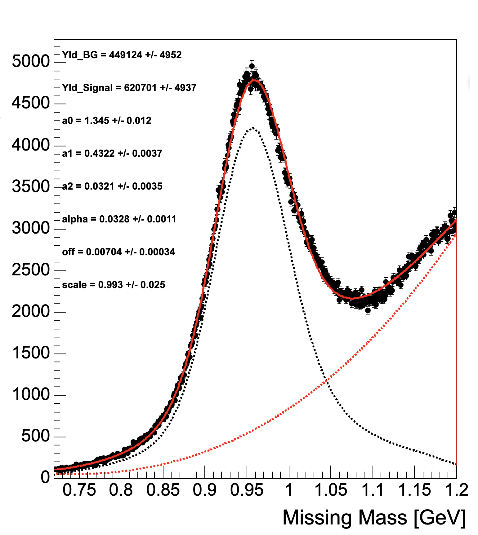
Figure 3: An sPlot fit of the invariant mass of $ep\to e^{\prime}\pi^{+}X$ in the region of the neutron missing mass. The background is fitted with a third order Chebyshev polynomial function. The parameters Yld_BG relate to the background yield, with a1, a2 and a3 the Chebyshev polynomial coefficients. The neutron signal is fitted using a simulated template. The parameter Yld_Signal relates to the neutron signal yield. Three parameters, alpha, off, scale, allow to convolute the simulated model to represent the data. The parameter off allows to offset the mean of the distribution, with the scale parameter scaling the width. The parameter alpha allows to convolve the simulated model with an additional Gaussian to better fit the data.

The methodology of Section 2 was applied to the sWeights produced by the fit in Figure 3. We employed a double density ratio with two gradient boosted decision tree (GBDT) steps with a max depth of ten each implemented with the scikit-learn library [19]. The denominator sample was composed of all unweighted events and the numerator sample was composed of all events weighted using the neutron signal sWeights. The GBDTs were trained on the reconstructed neutron spherical momentum components.

Figure 4 shows a comparison of all events, and the same events weighted by the sWeights and the drWeights, for each of the reconstructed momentum magnitude, polar and azimuthal angles. The uncertainties were propagated from the original sWeights. Figure 4 also shows the pull between the two distributions defined as the difference between the bin values for the two distributions divided by the sum squared of their uncertainties. The correlation between momentum and polar angle, and polar and azimuthal angles are also shown. Overall, the distributions are well reproduced when applying the drWeights, as shown by the fact that the pull is consistent with one in nearly all 1 dimensional bins. Accurately converting the sWeights to positive definite probabilities could then have many applications. The drWeights could then be used, for example, to train a machine learning algorithm to model the neutron detection efficiency as a function of all three momentum components reconstructed from the missing four-vector.

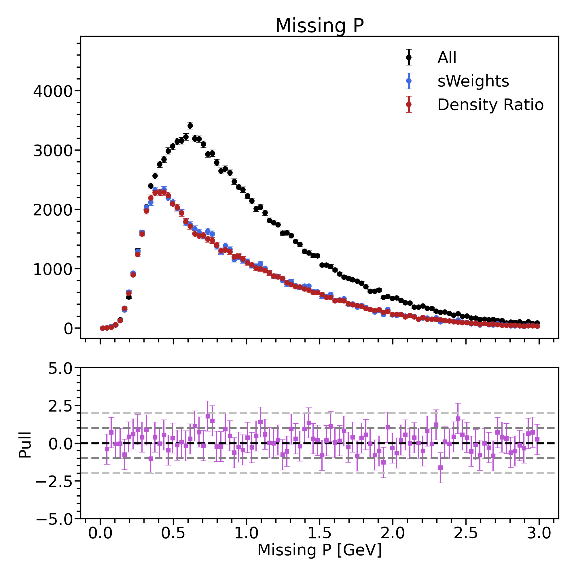
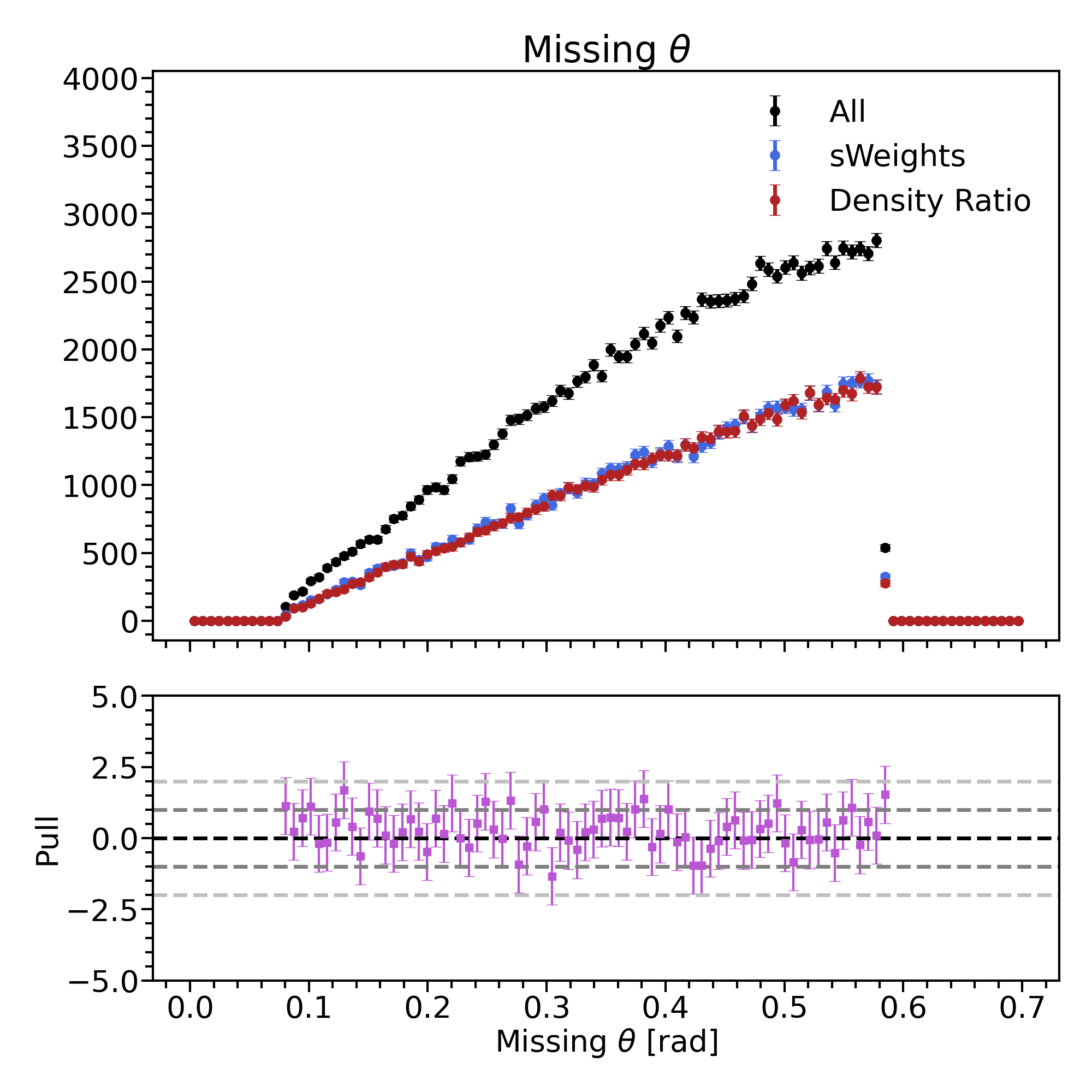
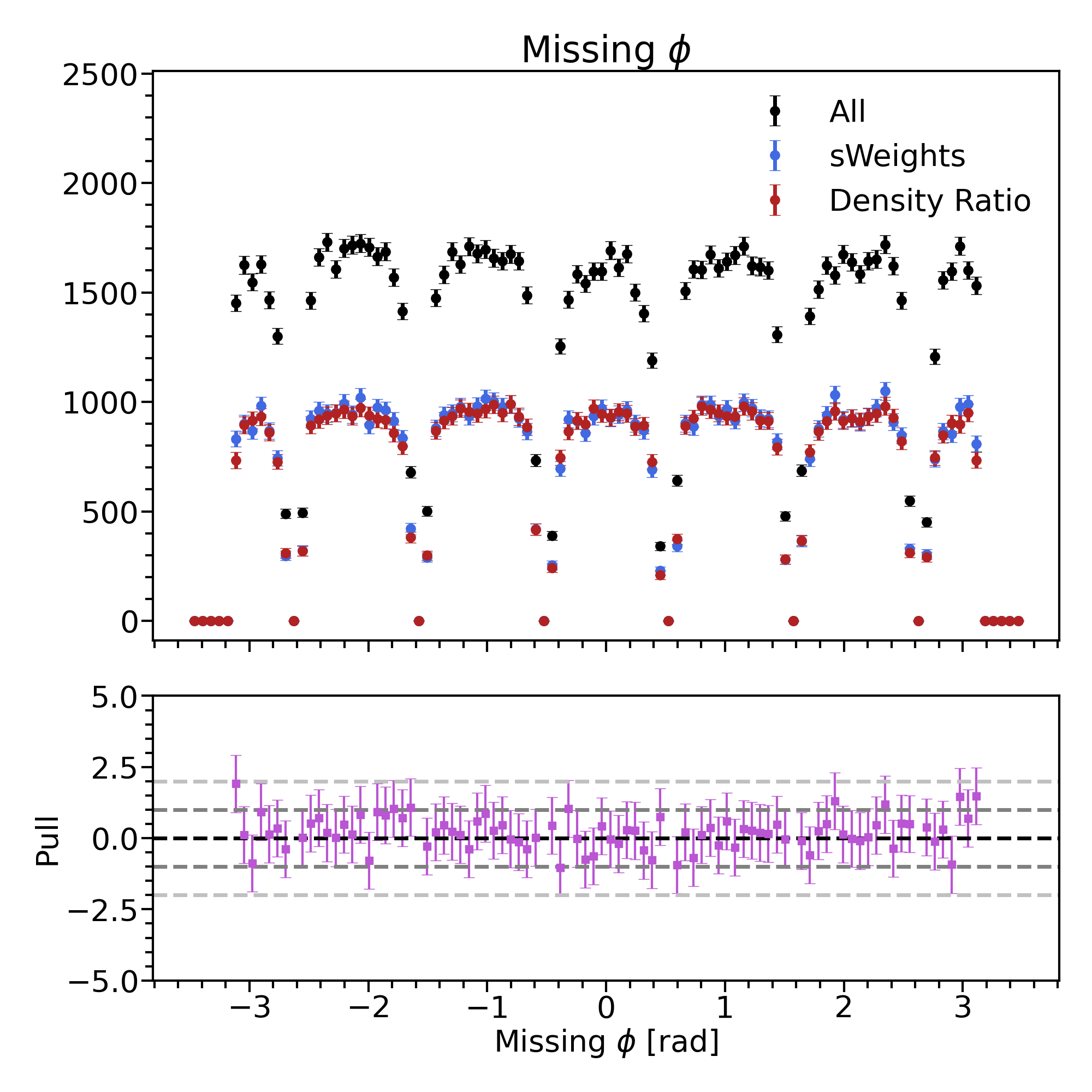
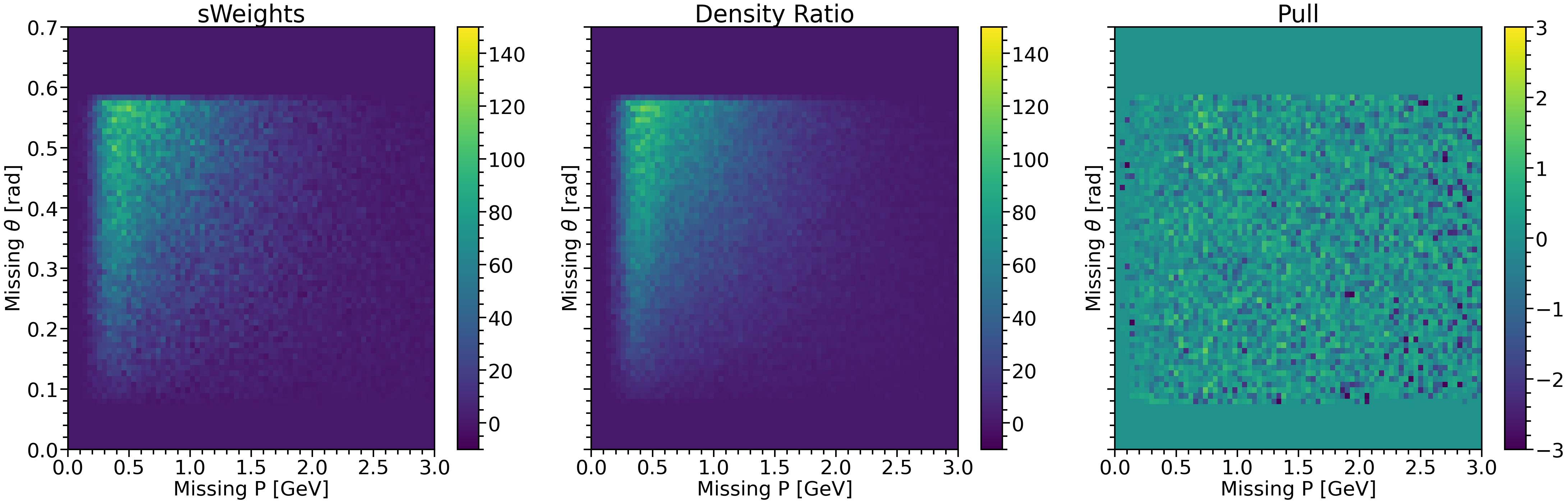
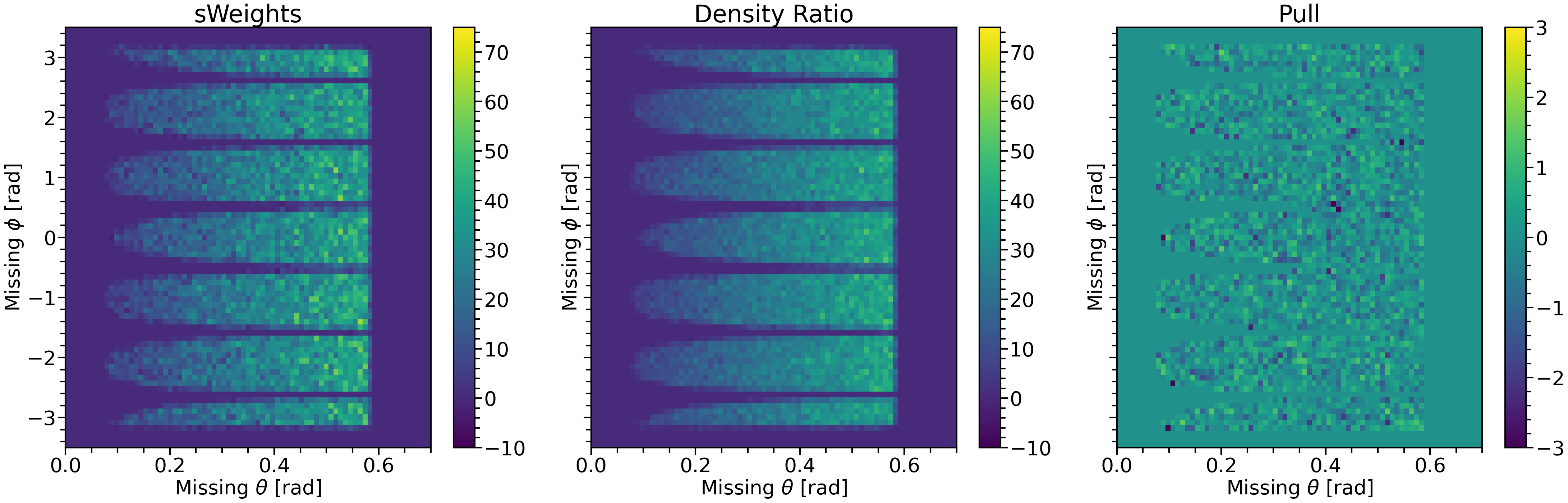
Figure 4: Top row: A comparison of all events (black) and all events weighted by the sWeights (blue) or by the drWeights (red) using the density ratio method. The comparison is made for each of the missing momentum (left), polar angle ($\theta$, middle) and azimuthal angle ($\phi$, right). Middle Row: The momentum and the polar angle ($\theta$) correlation histogram weighted using the sWeights (left) or drWeights (middle) and the pull between the two (right). Bottom Row: The polar angle ($\theta$) and azimuthal angle ($\phi$) correlation histogram weighted using the sWeights (left) or drWeights (middle) and the pull between the two (right)

4 Conclusion And Outlook

The sPlot formalism is a useful tool to separate different event species in high energy and nuclear physics experimental data. However, the sWeights obtained using the sPlot technique have negative values which will lead to issues in training and poor overall performance when using machine learning algorithms on data weighted with these sWeights.

Ref. [12] introduced a methodology based on density ratio estimation to resample weights from Monte Carlo event generators so as to avoid negative weights whilst preserving their statistical properties. The key point is that setting up the training sample so as to learn the density ratio of the weights, which in turn allows to resample these, means that the binary cross entropy loss function is not detrimentally affected by negative weights (c.f. Equation 3). This article has detailed how sWeights can be converted to probabilities using density ratio estimation, producing drWeights. We further detailed how gradient boosted decision trees are particularly well suited to converting sWeights. Moreover double density ratios, where a subsequent reweighting is applied to fine-tune the distributions, produces particularly robust weights for the dataset.

Two case studies were presented, one based on a toy example and another on experimental data from the CLAS12 detector. These demonstrated how density ratios can be applied to accurately convert sWeights and preserve their statistical properties. The first case study also highlighted the advantages of using decision trees, namely a non negligible increase in prediction rate and good performance with decreased data sizes and signal to background ratios. The latter is an important consideration as experimental data is limited and may have irreducible signal to background ratios. It is generally beneficial to have several options of learning algorithms to choose from depending on the dataset and task at hand.

The methodology presented in this article can be used for many applications of machine learning to experimental data in high energy and nuclear physics. In general, it is necessary to disentangle the distributions of different event species in experimental data to be able to use the distributions of specific species to train a machine learning algorithm. The second case study presented here detailed how converting sWeights to drWeights could be applied as a useful first step to learning the neutron detection efficiency in the CLAS12 forward detector. The mass of missing particles in $ep\to e^{\prime}\pi^{+}X$ can be fitted to distinguish the neutron signal from the background. The signal sWeights can then be converted to drWeights as described in Section 3.2. These converted weights can then be used in training a binary classification algorithm to model the CLAS12 forward detector neutron detection efficiency. Previous work has demonstrated the use of density ratio estimation via binary classification to model detector efficiency from simulation [10, 11]. The method to obtain drWeights described in this article could be a first step to modelling detector efficiency from experimental data. In general, many such applications will exist and require to accurately convert sWeights to positive definite probabilities as done here.

Finally we note that for general analysis, for example extracting an asymmetry from a background subtracted distribution, sWeights themselves will still provide a more reliable method. The goal here is not to replace sWeights in these circumstances, only in the cases such as machine learning training where positive definite probabilities are required.

References

- [1] Muriel Pivk and Francois R. Le Diberder. SPlot: A Statistical tool to unfold data distributions. Nucl. Instrum. Meth. A, 555:356–369, 2005.
- [2] Jeppe R. Andersen and Andreas Maier. Unbiased elimination of negative weights in monte carlo samples. The European Physical Journal C, 82(5):433, May 2022.
- [3] M. Borisyak and N. Kazeev. Machine learning on data with splot background subtraction. Journal of Instrumentation, 14(08):P08020, aug 2019.
- [4] Maxim Borisyak and N. Kazeev. Machine Learning on sWeighted Data. J. Phys. Conf. Ser., 1525(1):012088, 2020.
- [5] Liudmila Prokhorenkova, Gleb Gusev, Aleksandr Vorobev, Anna Veronika Dorogush, and Andrey Gulin. Catboost: unbiased boosting with categorical features. In S. Bengio, H. Wallach, H. Larochelle, K. Grauman, N. Cesa-Bianchi, and R. Garnett, editors, Advances in Neural Information Processing Systems, volume 31. Curran Associates, Inc., 2018.
- [6] Masashi Sugiyama, Taiji Suzuki, and Takafumi Kanamori. Probabilistic Classification, page 47–55. Cambridge University Press, 2012.
- [7] D Martschei, M Feindt, S Honc, and J Wagner-Kuhr. Advanced event reweighting using multivariate analysis. Journal of Physics: Conference Series, 368:012028, jun 2012.
- [8] Anders Andreassen and Benjamin Nachman. Neural networks for full phase-space reweighting and parameter tuning. Phys. Rev. D, 101:091901, May 2020.
- [9] Alex Rogozhnikov. Reweighting with boosted decision trees. In Journal of Physics: Conference Series, volume 762, page 012036. IOP Publishing, 2016.
- [10] Anders Andreassen, Patrick T. Komiske, Eric M. Metodiev, Benjamin Nachman, and Jesse Thaler. Omnifold: A method to simultaneously unfold all observables. Phys. Rev. Lett., 124:182001, May 2020.
- [11] D. Darulis, R. Tyson, D. G. Ireland, D. I. Glazier, B. McKinnon, and P. Pauli. Machine Learned Particle Detector Simulations. ArXiv e-prints, 2207.11254, 2022.
- [12] Benjamin Nachman and Jesse Thaler. Neural resampler for monte carlo reweighting with preserved uncertainties. Phys. Rev. D, 102:076004, Oct 2020.
- [13] V.D. Burkert, L. Elouadrhiri, K.P. Adhikari, S. Adhikari, M.J. Amaryan, D. Anderson, G. Angelini, et al. The CLAS12 spectrometer at Jefferson Laboratory. Nuclear Instruments and Methods in Physics Research Section A: Accelerators, Spectrometers, Detectors and Associated Equipment, 959:163419, 2020.
- [14] Hans Dembinski, Matthew Kenzie, Christoph Langenbruch, and Michael Schmelling. Custom orthogonal weight functions (cows) for event classification. Nuclear Instruments and Methods in Physics Research Section A: Accelerators, Spectrometers, Detectors and Associated Equipment, 1040:167270, 2022.
- [15] M. Kenzie. Cows and sweights source code. https://github.com/sweights/sweights, Accessed 09-11-2024.
- [16] Christoph Langenbruch. Parameter uncertainties in weighted unbinned maximum likelihood fits. The European Physical Journal C, 82(5):393, May 2022.
- [17] Yoav Freund and Robert E. Schapire. Experiments with a new boosting algorithm. In International Conference on Machine Learning, 1996.
- [18] Jerome Friedman. Greedy function approximation: A gradient boosting machine. The Annals of Statistics, 29, 11 2000.
- [19] F. Pedregosa, G. Varoquaux, A. Gramfort, V. Michel, B. Thirion, O. Grisel, M. Blondel, et al. Scikit-learn: Machine learning in python. Journal of Machine Learning Research, 12:2825–2830, 2011.
- [20] sklearn User Guide. https://scikit-learn.org/stable/modules/tree.html#mathematical-formulation, Accessed 09-11-2024.
- [21] Patrick T. Komiske, Eric M. Metodiev, and Jesse Thaler. Energy flow networks: deep sets for particle jets. Journal of High Energy Physics, 2019(1):121, Jan 2019.
- [22] Manzil Zaheer, Satwik Kottur, Siamak Ravanbakhsh, Barnabas Poczos, Russ R Salakhutdinov, and Alexander J Smola. Deep sets. In I. Guyon, U. Von Luxburg, S. Bengio, H. Wallach, R. Fergus, S. Vishwanathan, and R. Garnett, editors, Advances in Neural Information Processing Systems, volume 30. Curran Associates, Inc., 2017.
- [23] Martín Abadi, Ashish Agarwal, Paul Barham, Eugene Brevdo, Zhifeng Chen, Craig Citro, Greg S. Corrado, et al. TensorFlow: Large-scale machine learning on heterogeneous systems, 2015. Software available from tensorflow.org.
- [24] Diederik P Kingma and Jimmy Ba. Adam: A method for stochastic optimization. ArXiv e-prints, 1412.6980, 2014.
- [25] Hans Dembinski and Piti Ongmongkolkul et al. scikit-hep/iminuit, Dec 2020.
- [26] Derek I. Glazier and Richard Tyson. https://github.com/rtysonCLAS12/DR4sWeights_toy/, Accessed 09-11-2024.
- [27] Christoph Leemann, David Douglas, and Geoffrey Krafft. The continuous electron beam accelerator facility: Cebaf at the Jefferson Laboratory. Annu. Rev. Nucl. Part. Sci, 51:413–50, 12 2001.
- [28] Dudek, Jozef, Ent, Rolf, Essig, Rouven, Kumar, K. S., Meyer, Curtis, McKeown, R. D., Meziani, Zein Eddine, et al. Physics opportunities with the 12 gev upgrade at Jefferson Lab. Eur. Phys. J. A, 48(12):187, 2012.
- [29] G. Asryan, Sh. Chandavar, T. Chetry, N. Compton, A. Daniel, N. Dashyan, N. Gevorgyan, et al. The CLAS12 forward electromagnetic calorimeter. Nuclear Instruments and Methods in Physics Research Section A: Accelerators, Spectrometers, Detectors and Associated Equipment, 959:163425, 2020.
- [30] M. Ungaro, G. Angelini, M. Battaglieri, V.D. Burkert, D.S. Carman, P. Chatagnon, M. Contalbrigo, et al. The CLAS12 geant4 simulation. Nuclear Instruments and Methods in Physics Research Section A: Accelerators, Spectrometers, Detectors and Associated Equipment, 959:163422, 2020.