Fermionic Gaussian Testing and Non-Gaussian Measures via Convolution

Abstract

We explore the properties of fermionic convolution defined by fermionic Gaussian unitary. A key finding is the purity invariance of pure Gaussian states under this convolution. Leveraging this property, we propose an efficient protocol to test the fermionic Gaussianity of pure states by using 3 copies of the input states. Furthermore, we introduce a new family of measures called “Non-Gaussian Entropy,” designed to quantify the fermionic non-Gaussianity of states.

I Introduction

Exploring the boundary between classical and quantum computation is one of the most important problems in quantum science. One method is to study the classical simulation of quantum circuits. This method not only helps identify the quantum resources that support computational advantages in quantum systems, but also evaluates the efficacy and scalability of quantum information-processing proposals.

For example, the Gottesman-Knill theorem [1] shows that stabilizer circuits can be simulated in polynomial time on a classical computer. Stabilizer circuits are composed solely of stabilizer input states, Clifford gates (which map stabilizer states to stabilizer states) and Pauli measurement. This theorem emphasizes the importance of nonstabilizerness in achieving quantum computational advantage. The nonstabilizerness is also known as “magic” [2]. In addition, it has been shown that the amount of magic can be used to bound the classical simulation time of quantum circuits [3, 4, 5, 6, 7, 8, 9, 10].

One can also see this in continuous-variable bosonic systems, in which the bosonic Gaussian states and unitaries play an important role in quantum information and computation protocols [11] due to their desirable mathematical properties. It has been shown that bosonic Gaussian circuits which consist of Gaussian input states, Gaussian unitaries and Gaussian measurements, are easy to simulate classically [12]. This result indicates that the bosonic non-Gaussianity is a quantum resource necessary for quantum advantage, a result further evidenced by the fact that non-Gaussian states are shown to be useful in many other quantum information tasks [13, 14, 15, 16, 17, 18], such as the GKP code [19]. A resource theory of non-Gaussianity has been developed to characterize and understand the properties of these states in bosonic quantum computation [20, 21, 22, 23, 24, 25, 26, 27, 28, 29, 30, 31].

Another important paradigm for the classical simulation of quantum circuits is the matchgate, first introduced by Valiant [32]. It has been shown that quantum circuits composed of matchgates acting on nearest-neighboring qubits can be simulated efficiently on a classical computer [32, 33, 34, 35]. The connection between matchgate circuits and the theory of fermionic linear optics (or fermionic Gaussian unitaries) has been later explored in [33, 36, 34, 37]. The theory of fermionic linear optics has a number of applications, including Majorana fermions in quantum wires [38] and Kitaev’s honeycomb lattice model [39]. Supported by advancements in experimental platforms [40, 41, 42, 43], this theory is extremely applicable to a variety of information processing tasks.

Recent research extends the notion of magic from Clifford circuits to matchgate circuits [44]. It has been shown that all pure fermionic non–Gaussian states are magic states for matchgate computations, i.e., non–Gaussian states can be used to implement non-Gaussian gates under some conditions [44]. In addition, the measure of non-Gaussianity in matchagte computation has been studied in the classical simulation quantum circuits [45, 46, 47] in a similar way as the Clifford circuits, which also work well in a general resource theory.

To delve deeper into the realm of fermionic non-Gaussianity, we propose a systematic approach using fermionic convolution. This is motivated by the idea that Gaussian properties remain invariant under convolution. We define and study the notion of fermionic convolution, realized through fermionic Gaussian unitaries. The iterative application of fermionic convolution to any input state $\rho$ converges to a Gaussian state with the same covariance; we call this iterative-limit process fermionic Gaussification. We show that fermionic Gaussification maps a state to its closest Gaussian state in the relative entropy distance and establish that this distance decreases monotonically with each iterative convolution application. We also identify that fermionic Gaussification is a resource-destroying map in the resource theory of fermionic quantum computation.

We prove that fermionic convolution preserves the entropy of its input if and only if they are Gaussian states. Based on this property, we propose a new measure to quantify non-Gaussianity, which we call “Non-Gaussian Entropy.” We also consider the problem of testing for Gaussianity: property testing is a crucial area in quantum computation that entails assessing whether a given state or circuit has a certain property. For instance, separability testing is used to ascertain whether a state is separable [48, 49, 50, 51, 52]. Here, we propose a novel protocol based on fermionic convolution to test whether a state is Gaussian by using 3 copies of the input states.

I.1 Preliminaries

Let us consider a system of $n$ fermionic modes, with the corresponding creation $a^{\dagger}_{j}$ and annihilation $a_{j}$ operators for $j=1,...,n$. They satisfy the canonical anti-commutation relations (CAR)

$$\{a_{j},a_{k}^{\dagger}\}=\delta_{jk},\quad\{a_{j},a_{k}\}=0.$$ (I.1)

It is convenient to define $2n$ Hermitian Majorana operators $\set{\gamma_{j}}^{2n}_{j=1}$ defined as

$$\gamma_{2j-1}=a_{j}+a^{\dagger}_{j},\quad\gamma_{2j}=i(a_{j}-a^{\dagger}_{j}).$$ (I.2)

The operators $\set{\gamma_{j}}^{2n}_{i=j}$ are Hermitian, traceless and generate a Clifford algebra $\mathcal{C}_{2n}$ which satisfies the relation

$$\{\gamma_{j},\gamma_{k}\}=2\delta_{jk}I.$$ (I.3)

The Majorana operators $\set{\gamma_{j}}^{2n}_{j=1}$ can be represented by the product of Pauli operators by by the Jordan-Wigner transformation as follows

$$\gamma_{2j-1} =Z^{\otimes(j-1)}\otimes X\otimes I^{\otimes(n-j)},$$

$$\gamma_{2j} =Z^{\otimes(j-1)}\otimes Y\otimes I^{\otimes(n-j)},~{}~{}\forall j.$$

Given an ordered subset (multi-index) $J\subset[2n]$, we define $\gamma_{J}$ as the ordered product of the Majorana operators indexed by $J$. Specifically,

$$\gamma_{J}=\prod_{i\in J}\gamma_{i}.$$

We also use $j=|J|$ to denote the size of the subset $J$. Moreover, any linear operator $A\in\mathcal{C}_{2n}$ can be expressed as a linear combination of the Majorana operators as follows

$$A=\dfrac{1}{2^{n}}\sum_{J}A_{J}\gamma_{J},\quad A_{J}=\mathrm{Tr}(\gamma_{J}^{\dagger}A)\in\mathbb{C}.$$ (I.4)

If all coefficients $A_{J}$=0 with $|J|$ being odd, then $A$ is called even, i.e, it can be expressed as

$$A=\dfrac{1}{2^{n}}\sum_{J:|J|\equiv 0\mod 2}A_{J}\gamma_{J}.$$

For example, under the Jordan-Wigner transformation, $|1\rangle\langle 1|=(1-Z)/2$ is even since $Z=-i\gamma_{1}\gamma_{2}$, but $|0\rangle\langle 1|=(X+iY)/2=(\gamma_{1}+i\gamma_{2})/2$ is not. Moreover, the parity of the number of fermions is conserved by the action if an even operator $A$ as $A$ commutes with the fermionic number-parity operator $\gamma_{all}=\Pi^{2n}_{j=1}\gamma_{j}$. (See more details about the Clifford algebra $\mathcal{C}_{2n}$ in Appendix A.)

The covariance matrix $\Sigma_{\rho}$, or $\Sigma(\rho)$, of a state $\rho\in C_{2n}$ is the $2n\times 2n$ real, anti-symmetric matrix with entries

$$(\Sigma_{\rho})_{jk}=\frac{i}{2}\operatorname{Tr}\left[\rho[\gamma_{j},\gamma_{k}]\right].$$ (I.5)

It can be decomposed into the block-diagonal form by a real orthogonal transformation $R\in SO(2n)$, i.e,

$$\Sigma_{\rho}=R\bigoplus^{n}_{j=1}\left[\begin{array}[]{cc}0&\lambda_{j}\\ -\lambda_{j}&0\end{array}\right]R^{T}.$$ (I.6)

Fermionic Gaussian states $\rho$ are defined as even states of the following form

$$\rho=C\exp\left(\frac{i}{2}\gamma^{T}h\gamma\right),$$ (I.7)

where $\gamma$ abbreviates the vector $(\gamma_{1},\gamma_{2},...,\gamma_{2n})$, $(h_{jk})$ is a real antisymmetric matrix, and $C\in\mathbb{R}$ is a normalization factor. Fermionic Gaussian states represent the ground and thermal states of non-interacting fermionic systems. By block-diagonalizing the real, anti-symmetric matrix $h$, we can rewrite $\rho$ as

$$\rho=\frac{1}{2^{n}}\prod^{n}_{j=1}(1+i\lambda_{j}\tilde{\gamma}_{2j-1}\tilde{\gamma}_{2j}),$$

where $\tilde{\gamma}=R\gamma$ with $R$ being block-diagonalizing the matrix $h$, and $\lambda_{j}$ are the eigenvalues in the block diagonalization (I.6). Each $\lambda_{j}$ lies in the interval $[-1,1]$. For Gaussian pure states, each $\lambda_{j}\in\{-1,1\}$.

In the theory of fermionic quantum computation, a special role is played by those unitary transformations which are generated by Hamiltonians of non-interacting fermionic systems, i.e. Hamiltonians which are quadratic in Majorana fermion operators. Specifically,

$$U=\exp\left(\dfrac{1}{2}\gamma^{T}h\gamma\right),$$ (I.8)

where $h$ is a anti-symmetric matrix. These unitaries are known as fermionic Gaussian unitaries (or fermionic linear optics transformations). Conjugation by a Gaussian unitary effect ans automorphism of the algebra $\mathcal{C}_{2n}$ by rotating the Majorana operators ([34], Theorem 3),

$$U\gamma_{j}U^{\dagger}=\sum_{k}R_{jk}\gamma_{k},\quad R=\exp(2h)\in SO(2n).$$ (I.9)

More details are presented in Appendix B.

II Fermionic convolution

Let us begin by introducing the concept of a fermionic beam splitter, which mixes the Majorana operators of fermionic modes. This concept is inspired by the analogous device in bosonic systems, the bosonic beam splitter.

A fermionic beam splitter cting on $2n$ modes is represented by the Gaussian unitary operator

$$W_{\theta}=\exp\left(\dfrac{\theta}{2}\sum_{j=1}^{2n}\gamma_{j}\gamma_{2n+j}\right),$$ (II.1)

where $\gamma_{j}$ and $\gamma_{2n+j}$ are the Majorana operators on the fermionic modes. Then the fermionic beam splitter $W_{\theta}$ rotates the Majorana operators as follows

$$W_{\theta}\gamma_{j}W_{\theta}^{\dagger}=\cos\theta\gamma_{j}-\sin\theta\gamma_{2n+j},$$ (II.2)

$$W_{\theta}\gamma_{2n+j}W_{\theta}^{\dagger}=\sin\theta\gamma_{j}+\cos\theta\gamma_{2n+j},$$

for any $1\leq j\leq 2n$ and $\theta\in[-\pi,\pi]$. For $\theta=\pi/4$, it is called the balanced fermionic beam splitter. More discussion on the fermionic beam splitter can be found in Appendix C.

Definition 1 (Fermionic convolution).

The fermionic convolution of two even states $\rho$ and $\sigma$ with angle $\theta\in(-\pi,\pi)$ is

$$\rho\boxtimes_{\theta}\sigma=\operatorname{Tr}_{2}\left[W(\rho\otimes\sigma)W^{\dagger}\right],$$ (II.3)

where $\operatorname{Tr}_{2}\left[\cdot\right]$ denotes partial trace over the second register corresponding to the $n$ qubits of $\sigma$.

This fermionic convolution satisfies several elegant properties. For example, if both $\rho$ and $\sigma$ are Gaussian states, then $\rho\boxtimes\sigma$ is a Gaussian state. Moreover, it commutes with any Gaussian unitary $U_{G}$, i.e., $(U_{G}\rho U^{\dagger}_{G})\boxtimes_{\theta}(U_{G}\sigma U^{\dagger}_{G})=U_{G}(\rho\boxtimes_{\theta}\sigma)U^{\dagger}_{G}$ (see Appendix C for details of the proof). For simplicity, we focus on the case where $\theta=\pi/4$ throughout the main discussion, denoting $\boxtimes_{\pi/4}$ simply as $\boxtimes$.

Let us consider the iteration of the convolution $\boxtimes^{k}\rho$ for any integer $k$, which is defined as $\boxtimes^{k}\rho=(\boxtimes^{k-1}\rho)\boxtimes(\boxtimes^{k-1}\rho)$ and $\boxtimes^{0}\rho=\rho$. Based on the central limit theorem for fermionic convolution [53, 54], the iteration of the convolution $\boxtimes^{k}\rho$ will converge a Gaussian state with the same covariance. We define this transformation as fermionic Gaussification $\mathcal{G}(\rho)$, which maps any fermionic state $\rho$ to a Gaussian with the same covariance. Then $\lim_{k\to\infty}\boxtimes^{k}\rho=\mathcal{G}(\rho)$. For completeness, we also provide a proof of this central limit theorem with quantitative bound on the rate of convergence in Appendix D, which may be of independent interest.

In addition, we find that the fermionic Gaussification $\mathcal{G}(\rho)$ is the closest fermionic Gaussian state to the given even state $\rho$ with respect to the quantum relative entropy $D(\rho||\sigma)=\mathrm{Tr}(\rho\log\rho)-\mathrm{Tr}(\rho\log\sigma)$.

Proposition 2.

For any even state $\rho$, we have

$$\min_{\sigma_{G}\in\textbf{Gauss}}D(\rho||\sigma_{G})=D(\rho||\mathcal{G}(\rho))=S(\mathcal{G}(\rho))-S(\rho),$$ (II.4)

where Gauss denotes the set of all fermionic Gaussian states.

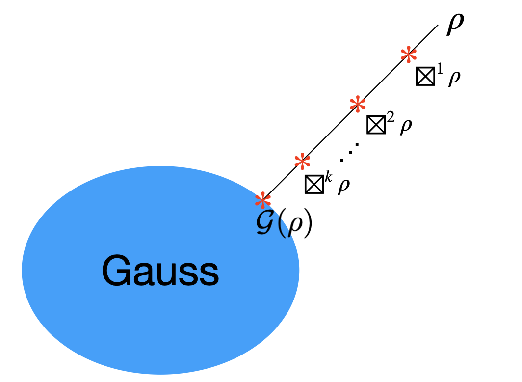
Figure 1: The Gaussification $\mathcal{G}(\rho)$ is the closest state to the states $\rho$ and $\boxtimes^{k}\rho$.

If we take the set Gauss as the set of free states $\mathcal{F}$ in the resource of fermionic quantum computation, then we can define the relative entropy of fermionic non-Gaussianity as

$$NG_{R}(\rho):=\min_{\sigma_{G}\in\textbf{Gauss}}D(\rho||\sigma_{G}),$$ (II.5)

which can also be written as $NG_{R}(\rho)=S(\mathcal{G}(\rho))-S(\rho)$ based on Proposition 2. It is easy to check that $NG_{R}$ satisfies the following nice properties. Hence, $NG_{R}$ is a measure of non-Gaussianity in the resource theory of fermionic quantum computation.

Proposition 3.

The following properties hold for the relative entropy of fermionic non-Gaussianity $NG_{R}$ ,

1. Faithfulness: $NG_{R}(\rho)\geq 0$ with equality iff $\rho$ is a fermionic Gaussian.

2. Gaussian-invariance: $NG_{R}(U_{G}\rho U^{\dagger}_{G})=NG_{R}(\rho)$ for any Gaussian unitary $U_{G}$.

3. Additivity under tensor product: $NG_{R}(\rho_{1}\otimes\rho_{2})=NG_{R}(\rho_{1})+NG_{R}(\rho_{2})$.

Recall that resource-destroying maps are one of the important concepts in the resource theory. A map $\lambda$ from states to states is called a resource-destroying map [55] if it satisfies the following two conditions: i) it maps all states to free states, i.e, $\lambda(\rho)\in\mathcal{F}$ for any quantum state $\rho$; ii) it fixes the free states, i.e., $\lambda(\sigma)=\sigma$ for any $\sigma\in\mathcal{F}$. The natural resource-destroying maps are known in resource theories such as coherence [56, 57], asymmetry [58], bosonic non-Gaussianity [22], and magic in the stabilizer quantum computation [59]. It is easy to check that the Gaussification $\mathcal{G}(\cdot)$ satisfies the conditions i) and ii) with $\mathcal{F}=\textbf{Gauss}$. So we have the following statement.

Proposition 4.

The Gaussification $\mathcal{G}(\cdot)$ is a (nonlinear) resource destroying map in the resource theory of fermionic quantum computation with Gauss being the set of free states.

Moreover, $\mathcal{G}(\rho)$ is also the Gaussification of self-convolution state $\boxtimes^{k}\rho$, i.e.,$\mathcal{G}(\boxtimes^{k}\rho)=\mathcal{G}(\rho)$. Moreover, the distance is monotonically decreasing, i.e., $D(\boxtimes^{k}\rho||\mathcal{G}(\rho))\geq D(\boxtimes^{k+1}\rho||\mathcal{G}(\rho))$ for any integer $k$. (See Figure. 1.) This comes from the following result, which we call the second law of thermodynamics for fermionic convolution (See the proof in Appendix C. ).

Theorem 5.

For any even state $\rho$, it holds that

$$S(\boxtimes^{k+1}\rho)\geq S(\boxtimes^{k}\rho),\forall k.$$ (II.6)

III Fermionic Gaussian test

We have studied the basic properties of fermionic convolution, which is defined through matchgate. Now, let us consider the applications of this fermionic convolution in fermionic Gaussian testing. The question is: give an pure fermionic state $\psi$, can we decide wether $\psi$ is a Gaussian not. If not, then $\psi$ is a non-Gaussian state, or a magic state in fermionic quantum computation, useful to generate a non-Gaussian gate [44].

We introduce a protocol to test fermionic Gaussianity utilizing three copies of the state. This protocol comprises two main steps: (1) fermionic convolution, and (2) a swap test to measure the overlap between the self-convolved state $\psi\boxtimes\psi$ and $\psi$. The detailed steps of the protocol are outlined in the following table.

The probability of acceptance in the above fermionic Gaussian test is equal to

$$\text{Pr}_{\text{accept}}(\psi)=\frac{1}{2}\left[1+\bra{\psi}\psi\boxtimes\psi\ket{\psi}\right].$$ (III.1)

Theorem 6.

For any pure even state $\ket{\psi}$, the pure state is a Gaussian state if and only if the the probability of acceptance $\text{Pr}_{\text{accep}}(\psi)=1$.

This theorem is derived from the property of purity invariance under fermionic convolution. Specifically, for a pure even state $\psi$, the state $\psi\boxtimes\psi$ remains pure if and only if $\psi$ is a fermionic Gaussian state. This is proved in Appendix C. Moreover, by the Choi isomorphism, we can also extend the Gaussianity testing from states to unitaries. (See Appendix G.)

It is worth recalling that separability testing relies on the principle that a pure bipartite state $\ket{\phi}_{AB}$ is separable if and only if the reduced state $\rho_{A}$ is pure. This principle underpins the well-known entanglement measure, entanglement entropy, defined as $S(\rho_{A})$. Similarly, we can use the fermionic Gaussianity test to introduce a new measure to quantify fermionic non-Gaussianity, which we term “non-Gaussian entropy.”

Non-Gaussian entropy: Non-Gaussian entropy of any pure even state $\psi$ is defined as

$$NG(\psi)=S(\psi\boxtimes\psi).$$ (III.2)

Theorem 7.

The Non-Gaussian entropy for even stats $\psi$ also satisfy the property (1)-(3) in  Proposition 3.

(See the proof in Appendix C). Hence, non-Gaussian entropy can be used a resource measure in the theory of fermionic quantum computation.

We can also generalize the non-Gaussian entropy to the higher-order case. The $k$-th order non-Gaussian entropy

$$NG^{(k)}(\psi)=S(\boxtimes^{k}\psi),$$ (III.3)

which also satisfies the above three properties in Theorem 7. Thus, these form a new family of measures for quantifying fermionic non-Gaussianity. Furthermore, the asymptotic behavior of higher-order non-Gaussian entropy approaches the relative entropy of non-Gaussianity $NG_{R}$, i.e,

$$\lim_{k\to\infty}NG^{(k)}(\psi)=NG_{R}(\psi).$$ (III.4)

This indicates that non-Gaussian entropy can be considered as a finite-shot approximation of the relative entropy of non-Gaussianity.

Example: Let us consider a family of quantum states on a 4-qubit system,

$$\ket{\psi_{\phi}}=\frac{1}{2}\left(\ket{0000}+\ket{0011}+\ket{1100}+e^{i\phi}\ket{1111}\right),$$ (III.5)

with $\phi\in(0,2\pi)$. Theses state are shown to be magic states for the fermionic quantum computation [44]. Here, we compute the non-Gaussian entropy and the relative entropy of non-Gaussianity for these states, plotting the results in Fig. 2. Notably, all entropies are nonzero for all $\phi\in(0,2\pi)$, and $NG^{(3)}(\psi_{\phi})$ closely approximates $NG^{(\infty)}(\psi_{\phi})$, suggesting that $NG^{(k)}$ for a finite $k$ can serve as a good approximation of the relative entropy of non-Gaussianity.

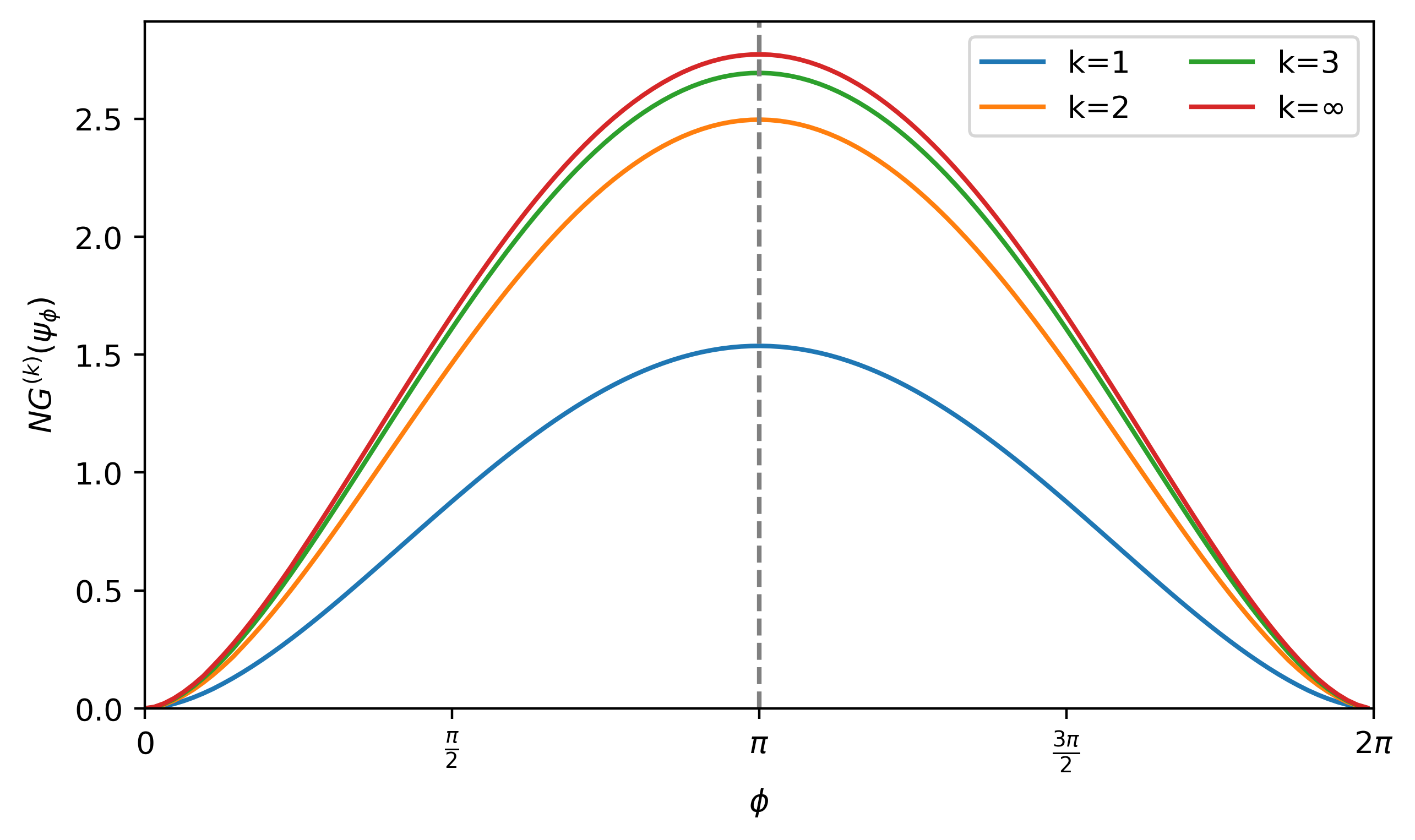
Figure 2: Non-Gaussian entropy $NG^{(k)}(\psi_{\phi})$ of the $4$-qubit state $\psi_{\phi}$ in (III.5) for $k=1,2,3,\infty$.

Remark: We can also replace the quantum entropy $S(\rho)$ by the quantum Rényi entropy $S_{\alpha}(\rho)=\frac{1}{1-\alpha}\log\operatorname{Tr}\left[\rho^{\alpha}\right]$. That is, we can define the $k$-th order, $\alpha$ Rényi non-Gaussian entropy $NG^{(k)}_{\alpha}(\psi)=S_{\alpha}(\boxtimes^{k}_{\alpha})(\psi)$, which is also good measure to quantify the fermionic non-Gaussianity (See Appendix C). To extend the non-Gaussian entropy to mixed states, we have two different forms depending on the choice of the set free states $\mathcal{F}$ for fermionic quantum computation. For $\mathcal{F}=\textbf{Gauss}$ as discussed in the main text, we can define the the $k$-th order non-Gaussian entropy as $NG^{(k)}(\rho)=S(\boxtimes^{k}\rho)-S(\rho)$, which also satisfies the properties in Proposition 3. If we choose $\mathcal{F}$ to be the convex hull of Gauss, then we can use the technique of convex roof to define the $k$-th order non-Gaussian entropy for mixed states $\tilde{NG}^{(k)}(\rho)=\min_{\rho=\sum_{i}\lambda_{i}\left|\psi_{i}\right\rangle\!\left\langle\psi_{i}\right|}\sum_{i}\lambda_{i}NG^{(k)}(\psi_{i})$, where the minimization is taken over all pure state decomposition of $\rho$. It not only satisfies the properties in Proposition 3 but also the convexity, i.e., $\tilde{NG}^{(k)}(\sum_{i}p_{i}\rho_{i})\leq\sum_{i}p_{i}\tilde{NG}^{(k)}(\rho_{i})$.

IV Conclusion and discussion

In this work, we have investigated fermionic convolution and its application in quantifying non-Gaussianity in fermionic quantum computation. These results provide a novel perspective on the study of magic for fermionic quantum computation.

This work also raises several intriguing questions for future exploration. For instance, although using only 3 copies provides an efficient Gaussianity test, it would be interesting to determine whether 3 copies are indeed optimal. In addition, a series of studies [59, 60, 61, 62, 63, 64, 65] have characterized stabilizer states through discrete convolution, highlighting the Gaussian nature of stabilizerness. This suggests potential for a unified framework for classically simulable states and circuits, leveraging their common Gaussian structures. Such a framework could pave the way for discovering new families of classically simulable quantum circuits by identifying new Gaussian (or quadratic) forms.

V Acknowledgments

We thank Arthur Jaffe, Weichen Gu, and Sasha Berger for helpful discussions. This work is supported in part by the ARO Grant W911NF-19-1-0302 and the ARO MURI Grant W911NF-20-1-0082.

Note: During the preparation of this manuscript, we became aware of another work studying fermionic convolution and the central limit theorem [66].

Here is an outline of the appendix: In Sec. A, we introduce the mathematical foundations of Clifford and Grassman algebra, paying special to the the Fourier transform. In Sec. B, we explore the Fourier coefficients by defining moments, cumulants, and applying these concepts to characterize fermionic Gaussian states and quantify the no-Gaussianity. In Sec. C, we provide detailed proofs for the desirable properties of fermionic convolution. In Sec. D, we focus on the central limit theorem for the fermionic convolution and provide a quantitative bound on the rate of convergence. In Sec. E, we explore the properties of the Gaussification map. In Sec. F, we study the the potential generalization of convolution to non-even states. In Sec. G, we extend the testing of Gaussianity from states to unitaries.

Appendix A Background in Clifford and Grassmann algebras

We review the mathematical background in the Clifford algebra $\mathcal{C}_{2n}$ over generators $\{\gamma_{1},\cdots,\gamma_{2n}\}$ and the Grassmann algebra $\mathcal{G}_{2n}$ over generators $\{\eta_{1},\cdots,\eta_{2n}\}$. For more details, see [67, 68, 37].

A.1 Clifford and Grassmann algebras

Definition A.1 (Clifford algebra).

A finitely-generated Clifford algebra $\mathcal{C}_{2n}$ over $2n$ generators $\gamma_{1},\cdots,\gamma_{2n}$ consists of complex polynomials over the generators $\gamma$ subject to the anti-commutation relation

$$\{\gamma_{j},\gamma_{k}\}=2\delta_{jk},\quad j,k=1,\cdots,2n.$$

In this work, we also require the generators to be self-adjoint $\gamma_{j}^{*}=\gamma_{j}$. The algebra $\mathcal{C}_{2n}$ is $2^{2n}$-dimensional, with basis elements $\{\gamma_{J}:J\subset[2n]\}$ indexed by ordered subsets of $[2n]=\{1,\cdots,2n\}$ according to

$$\gamma_{J}=\gamma_{J_{1}}\gamma_{J_{2}}\cdots\gamma_{J_{|J|}}.$$

Note that self-adjointness of the generators is not a standard requirement in mathematics literature, so strictly speaking $\mathcal{C}_{2n}$ should be denoted the Majorana algebra. However, we will continue referring to $\mathcal{C}_{2n}$ as the Clifford algebra in this context in line with the terminology used in [54].

The Jordan-Wigner transform faithfully represents the Clifford algebra $\mathcal{C}_{2n}$ on the space $\mathcal{H}_{n}$ of $n$-qubit operators. The self-adjoint generators $\gamma_{j}^{*}=\gamma_{j}$ are represented as Hermitian Pauli operators, and the generated basis $\{\gamma_{J}\}$ is orthonormal under the Hilbert-Schmidt inner product

$$\langle A,B\rangle=\dfrac{1}{2^{n}}\mathrm{Tr}(A^{\dagger}B),\quad A,B\in\mathcal{H}_{n}.$$ (A.1)

Using this representation, we identify

$$\mathrm{Tr}(1_{\mathcal{C}_{2n}})=2^{n}\quad\mathrm{Tr}(\gamma_{J\neq\emptyset})=0.$$ (A.2)

Definition A.2 (Grassmann algebra).

A finitely generated Grassmann algebra $\mathcal{G}_{2n}$ over $2n$ generators $\eta_{1},\dots,\eta_{2n}$ consists of complex polynomials over $\eta$ subject to the multiplication rules:

$$\eta_{a}^{2}=0,\quad\{\eta_{a},\eta_{b}\}=0\text{ when }a\neq b.$$

The Grassmann basis $\{\eta_{J}\}$ is defined analogously to the Clifford case.

We use the orthonormal representation of $2n$ Grassmann generators on a $2n$-qubit Hilbert space $\mathcal{H}_{2n}$ as

$$\eta_{j}=Z^{\otimes j-1}\otimes\sigma^{+}\otimes I^{\otimes 2n-j},\forall j\in[2n].$$ (A.3)

Here $\sigma^{+}=\sqrt{2}\,|0\rangle\langle 1|$, which satisfies $Z\sigma^{+}=-\sigma^{+}Z=\sigma^{+}$. Note that the $2n$ generators only span a subspace of $\mathcal{H}_{2n}$. The generated basis $\{\eta_{J}\}_{J\subset[2n]}$ is orthonormal under the Hilbert-Schmidt product

$$\langle A,B\rangle=\dfrac{1}{2^{2n}}\mathrm{Tr}(A^{\dagger}B).$$ (A.4)

Recall that a $*$-representation of an algebra is one on which the $*$-operator is represented by conjugate-transpose. Unlike the Clifford case, there is no faithful $*$-representation of the Grassmann algebra with Hermitian generators $\eta_{j}^{\dagger}=\eta_{j}$. To see this, $\eta_{j}^{*}=\eta_{j}$ implies that the $*$-representation of generators must have real eigenvalues, but nilpotency $\eta_{j}^{*}\eta_{j}=0$ imply that the representation must be trivial. In light of this, we cannot directly use the Hilbert-Schmidt formula to define the inner product, which are instead defined as

$$\langle\eta_{J},\eta_{K}\rangle=\dfrac{1}{2^{2n}}(-1)^{|J|(|J|-1)/2}\mathrm{Tr}(\eta_{J}\eta_{K}),\quad\|A\|_{2}^{2}=\langle A,A\rangle.$$ (A.5)

This is the Hilbert-Schmidt product upon manually enforcing $\eta_{j}^{\dagger}=\eta_{j}$. Using this representation, we identify

$$\mathrm{Tr}(1_{\mathcal{G}_{2n}})=2^{2n},\quad\mathrm{Tr}(\eta_{J\neq\emptyset})=0.$$ (A.6)

We also need the anti-commuting tensor product when dealing with transformation between algebras.

Definition A.3 (Anti-commuting tensor product).

Given two finitely generated algebras $\mathcal{A}=\langle\{a_{1},\cdots,a_{n}\}\rangle$ and $\mathcal{B}=\langle\{b_{1},\cdots,b_{m}\}\rangle$, the anti-commuting tensor product $\mathcal{A}\otimes_{f}\mathcal{B}$ is is generated by

$$\{a_{j}\otimes_{f}1:1\leq j\leq n\}\cup\{1\otimes b_{k}:1\leq k\leq m\}.$$ (A.7)

Multiplication is defined by the following relation,

$$(a_{j}\otimes_{f}1)(1\otimes_{f}b_{k})=-(1\otimes_{f}b_{k})(a_{j}\otimes_{f}1).$$ (A.8)

To simplify notation, we typically equate $a_{j},b_{k}$ with their equivalents in $\mathcal{A}\otimes_{f}\mathcal{B}$, leading to the expression $a_{j}b_{k}=-b_{k}a_{j}$ as shown in equation (A.8). We resort to the full notation only when explicit clarification of spaces is necessary.

Definition A.4 (Even subspace).

The even subspace (subalgebra) $\mathcal{A_{E}}$ of a finitely-generated algebra $\mathcal{A}$ is spanned by the products of an even number of generators i.e. all nontrivial terms in the polynomial expansion are of even degree.

In this work, we will focus the even space with following isomorphism

$$\mathcal{A}\otimes_{f}\mathcal{B_{E}}\cong\mathcal{A}\otimes\mathcal{B_{E}},$$ (A.9)

where $\mathcal{A}$ and $\mathcal{B}$ could be either the Clifford algebra $\mathcal{C}_{2n}$ or the Grassmann algebra $\mathcal{G}_{2n}$. This identification exploits the property that even elements $b_{K}$ commute with $a_{J}$ irrespective of using $\otimes$ or $\otimes_{f}$:

$$(a_{J}\otimes_{f}1)(1\otimes b_{K})\in\mathcal{A}\otimes_{f}\mathcal{B_{E}}\leftrightarrow a_{J}\otimes b_{K}\in\mathcal{A}\otimes\mathcal{B_{E}}$$ (A.10)

The reason we primarily focus on the even subspace is that the desirable mathematical properties of fermion operations are typically defined in $\mathcal{A}\otimes_{f}B$ but, operationally, we can only access the algebra $\mathcal{A}\otimes\mathcal{B}$.

A.2 Grassmann-Clifford Fourier transform

The Clifford algebra is intricately related to the Grassmann algebra by a Fourier transform which effectively corresponds to a formal relabeling of generators. Here, we recount the Grassmann algebra and consider this Fourier transform, which to the best of our knowledge appeared under the name of “moment-generating function” in [54].

Recall that the classical Fourier transform is the integral with respect to kernel $e^{i\mathbf{t}\cdot\mathbf{x}}$ as follows

$$\mathcal{F}[f](\mathbf{t})=\int e^{i\mathbf{t}\cdot\mathbf{x}}f(\mathbf{x})\,d\mathbf{x}.$$ (A.11)

Hence, we consider the following kernel in the definition of the Grassman-Clifford Fourier transform,

$$e^{F}\quad\text{with}~{}F:=\gamma^{T}\eta=\sum_{j}\gamma_{j}\eta_{k}\in\mathcal{C}_{2n}\otimes_{f}\mathcal{G}_{2n}.$$ (A.12)

The kernel expands into the algebra basis as

$$e^{F}=\sum_{J}(-1)^{j(j-1)/2}\eta_{J}\gamma_{J}=\sum_{J}\eta_{J}\gamma_{J}^{\dagger}.$$ (A.13)

where $j\equiv|J|$ is the size (degree) of the index (monomial). To see this, the polynomial expansion of $e^{F}$ is trivial after the $2n$-th degree. In the $k$-th degree (in $\gamma$ or $\eta$), the $1/k!$ Taylor coefficient cancels with the $k!$ ways of picking nontrivial terms across identical products, and reordering $\eta_{J_{1}}\gamma_{J_{1}}\cdots\eta_{J_{j}}\gamma_{J_{j}}$ into $\eta_{J}\gamma_{J}$ requires $j(j-1)/2$ swaps.

Denote by $\mathrm{Tr}_{\mathcal{C}}$ and $\mathrm{Tr}_{\mathcal{G}}$ the partial trace over the Clifford and Grassmann algebras, respectively, then

$$\Xi_{A}(\eta) =\mathcal{F}[A](\eta)=\mathrm{Tr}_{\mathcal{C}}\left(e^{F}A\right)=\dfrac{1}{2^{n}}\sum_{J}A_{J}\,\mathrm{Tr}_{\mathcal{C}}(\eta_{J}\gamma_{J}^{\dagger}\gamma_{J})=\sum_{J}A_{J}\eta_{J},$$ (A.14)

is the Grassman-Clifford Fourier transform. The conjugate action of Gaussian unitaries can be rewritten in the Grassmann formalism as

$$\Xi_{UAU^{\dagger}}(\eta)=\Xi_{A}(R\eta),$$ (A.15)

where $\Xi_{A}(R\eta)$ means substituting $\eta_{j}\mapsto\sum_{k}R_{jk}\eta_{k}$ in the expression of $\Xi_{A}(\eta)$.

Appendix B Characterization of Gaussianity by Fourier coefficients

In this section, we introduce Fourier coefficients, including moments and cumulants, for the fermionic system. These coefficients will be used to characterize fermionic Gaussian operators and quantify non-Gaussianity.

B.1 Moments and cumulants

The moments and cumulants of a state $\rho\in\mathcal{C}_{2n}$ are defined similarly to their classical statistics counterparts: moments are overlaps with basis projective operators, while cumulants are specific combinations of moments that are additive under convolution.

Definition B.1 (Moments).

Given a multi-index $J\subset[2n]$, the $J$-th moment of a $n$-qubit state $\rho\in\mathcal{C}_{2n}$ is

$$\rho_{J}=\mathrm{Tr}(\gamma^{\dagger}_{J}\rho).$$ (B.1)

The moment-generating operator (or function) $\Xi_{\rho}\in\mathcal{G}_{2n}$ is just the Fourier transform of $\rho$:

$$\Xi_{\rho}(\eta)=\sum_{J}\rho_{J}\eta_{J}.$$ (B.2)

Note that the orthonormality of $\{\gamma_{J}\}$ also implies

$$\rho=\dfrac{1}{2^{n}}\sum_{J}\rho_{J}\gamma_{J}\in\mathcal{C}_{2n}.$$ (B.3)

Any state is uniquely determined by the moments $\set{\rho_{J}}$. Since $i^{|J|}\gamma_{J}$ is a Hermitian with eigenvalues $\pm 1$, $|\rho_{J}|=|\operatorname{Tr}\left[\gamma^{\dagger}_{J}\rho\right]|\leq 1$. The orthonormal moment expansion equation B.3 also implies

$$\sum_{J\subset[2n]}|\rho_{J}|^{2}=2^{n}\operatorname{Tr}\left[\rho^{2}\right].$$

It is convenient to define the degree-dependent moment weight, which we will prove to be a Gaussian unitary-invariant scalar.

Definition B.2 (Moment weight).

Given a state $\rho$, the $k$-th moment weight is

$$W_{k}(\rho)=\sum_{|J|=k}|\rho_{J}|^{2}.$$ (B.4)

And the total moment weight is

$$I_{M}(\rho)=\sum^{2n}_{k=0}jW_{k}(\rho).$$ (B.5)

The total moment weight is also called sensitivity [69], which has been shown to be useful in the study of quantum circuit complexity.

Proposition B.1.

The $k$-th moment weight is Gaussian unitary-invariant: for every integer $0\leq k\leq 2n$:

$$W_{k}(U_{G}\rho U^{\dagger}_{G})=W_{k}(\rho).$$ (B.6)

Consequently, the total moment weight is also preserved,

$$I_{M}(U_{G}\rho U^{\dagger}_{G})=I_{M}(\rho).$$ (B.7)

Proof.

Fixing $0\leq k\leq 2n$, consider the $k$-th order tensor $(\Sigma^{(k)}_{\rho})_{l_{1},...,l_{k}}$ with $l_{i}\in[2n]$,

$$(\Sigma^{(k)}_{\rho})_{l_{1},...,l_{k}}=\begin{cases}\rho_{l_{1},..,l_{k}},&\text{if }l_{1},..,l_{k}\text{ are all different},\\ 0,&\text{otherwise.}\end{cases}$$

It is easy to see that $\left\lVert\Sigma^{(k)}_{\rho}\right\rVert^{2}_{2}:=\sum_{l_{1},..,l_{k}}|(\Sigma^{(k)}_{\rho})_{l_{1},...,l_{k}}|^{2}=W_{k}(\rho)$. We need to show that $\left\lVert\Sigma^{(k)}_{\rho}\right\rVert^{2}_{2}=\left\lVert\Sigma^{(k)}_{U_{G}\rho U^{\dagger}_{G}}\right\rVert^{2}_{2}$ for any Gaussian unitary $U_{G}$ which corresponds to a generator rotation $R$ such that $U_{G}\gamma U_{G}^{\dagger}=R\gamma$. Then

$$(\Sigma^{(k)}_{U_{G}\rho U^{\dagger}_{G}})_{l_{1},...,l_{k}}=\sum_{j_{1},..,j_{k}}\rho_{j_{1}...,j_{k}}\prod^{k}_{i}R_{j_{i},l_{i}}=\sum_{j_{1},..,j_{k}}(\Sigma^{(k)}_{\rho})_{l_{1},...,l_{k}}M_{(j_{1},...,j_{k}),(l_{1},...,l_{k})},$$ (B.8)

where $M_{(j_{1},...,j_{k}),(l_{1},...,l_{k})}=\prod^{k}_{i}R_{j_{i},l_{i}}\cong R^{\otimes k}$ is a $(2n)^{k}\times(2n)^{k}$ rotation matrix since $R$ is orthogonal. Thus, the weights of $\Xi_{\rho}(\eta)$ by each degree is equal to the weights of $\Xi_{U\rho U^{\dagger}}(\eta)=\Xi_{\rho}(R\eta)$ by degree since the degree-$k$ weight vector (tensor) $\Sigma^{(k)}_{\rho}$ undergoes rotation by $R^{\otimes k}$ under the unitary algebra automorphism $\eta\mapsto R\eta$. ∎

Definition B.3 (Cumulants).

Given a state $\rho$, the cumulant-generating operator (or function) $\Psi_{\rho}\in\mathcal{G}_{2n}$ is

$$\Psi_{\rho}(\eta)=\log\,\Xi_{\rho}(\eta)=\sum_{k=1}^{2n}(-1)^{k+1}\dfrac{(\Xi_{\rho}-1_{\mathcal{G}_{2n}})^{k}}{k}=\sum_{J}\kappa^{\rho}_{J}\eta_{J},$$ (B.9)

where $\kappa^{\rho}_{J}$ is the $J$-th cumulant of $\rho$.

Note that the cumulant-generating element of a quantum state always exists because $\Xi_{\rho}-1_{\mathcal{G}}$ is nilpotent with degree at most $2n$. Additionally, note that from definition the quadratic cumulants and moments concur for even $\rho$:

$$\rho_{J}=\kappa^{\rho}_{J},\quad\forall J\subset[2n]~{}~{}\text{with}~{}~{}|J|=2.$$ (B.10)

Similar to the moment weight, we can also define the cumulant weight.

Definition B.4.

Given a state $\rho$, the $j$-th cumulant weight is

$$K_{j}(\rho)=\sum_{|J|=j}|\kappa^{\rho}_{J}|^{2}.$$ (B.11)

And the total cumulant weight is

$$K(\rho)=\sum_{j}jK_{j}(\rho).$$ (B.12)

Based on the equivalence of the second order moments and cumulants in (B.10), we have the equivalence of the corresponding weight $W_{2}(\rho)=K_{2}(\rho)$ for even states $\rho$.

Proposition B.2.

Given two even states $\rho$ and $\sigma$, we have

$$\Psi_{\rho\otimes\sigma}=\Psi_{\rho}\otimes 1+1\otimes\Psi_{\sigma}.$$ (B.13)

Thus, for even states $\rho$ and $\sigma$, the cumulant weight is additive, i.e.,

$$K_{j}(\rho\otimes\sigma)=K_{j}(\rho)+K_{j}(\sigma).$$ (B.14)

Proof.

Because $\Xi_{\rho\otimes\sigma}=\Xi_{\rho}\otimes\Xi_{\sigma}$, we have $\Psi_{\rho\otimes\sigma}=\log(\Xi_{\rho}\otimes\Xi_{\sigma})=\log\Xi_{\rho}\otimes 1+1\otimes\log\Xi_{\sigma}=\Psi_{\rho}\otimes 1+1\otimes\Psi_{\sigma}$. ∎

The proof above can be relaxed to only requiring $\sigma$ to be even; we require both inputs to be even for simplicity.

Proposition B.3.

The $j$-th cumulant weight is Gaussian unitary-invariant, i.e.,

$$K_{j}(U_{G}\rho U^{\dagger}_{G})=K_{j}(\rho).$$ (B.15)

Thus the total cumulant weight is also preserved,

$$K(U_{G}\rho U^{\dagger}_{G})=K(\rho).$$ (B.16)

Proof.

The proof is similar to that of Proposition B.1. For cumulants, we have

$$\Psi_{U\rho U^{\dagger}}(\eta)=\log[\Xi_{U\rho U^{\dagger}}(\eta)]=\log[\Xi_{\rho}(R\eta)]=(\log\Xi_{\rho})(R\eta)=\Psi_{\rho}(R\eta).$$

This is because $\eta\mapsto R\eta$ is an automorphism of the algebra, and algebra automorphisms commutes with all algebraic operations defined using addition, scalar multiplication, and algebra multiplication. Here $\varphi$ is an automorphism means that $\varphi(ab)=\varphi(a)\varphi(b)$. In particular, the Grassmann logarithm of the Fourier transform of states, defined as a finite power series  (B.9), is an algebraic operation. Applying the same argument to $\Psi_{\rho}(R\eta)$ demonstrates that the weights of $\Psi_{U\rho U^{\dagger}}(\eta)=\Psi_{\rho}(R\eta)$ and $\Psi_{\rho}(\eta)$, measured by degree, are identical.

∎

B.2 Gaussian states and unitaries

Recall that Gaussian states are the ground or thermal states of quadratic Hamiltonians, that is,

$$\rho=C\exp\left(\frac{i}{2}\gamma^{T}h\gamma\right),$$ (B.17)

where $(h_{jk})$ is a real, antisymmetric matrix and $C$ is a normalization constant. We will first show that the Fourier transform of the Gaussian state is also Gaussian. The covariance matrix of any state $\rho$ is defined as

$$(\Sigma_{\rho})_{jk}=\frac{i}{2}\operatorname{Tr}\left[\rho[\gamma_{j},\gamma_{k}]\right]=-i\mathrm{Tr}[(\gamma_{j}\gamma_{k})^{\dagger}\rho].$$ (B.18)

Since $h$ is a real, antisymmetric matrix, by a standard result in the matrix theory [70], there exists a rotation $R\in SO(2n)$ such that

$$R^{T}hR=h_{D}=\bigoplus_{j=1}^{n}\begin{bmatrix}0&\nu_{j}\\ -\nu_{j}&0\end{bmatrix},\quad\nu_{j}\geq 0.$$ (B.19)

Using a Gaussian unitary $U_{G}$ to implement the rotation, we can diagonalize $\rho$ according to

$$\rho_{D}:=U_{G}\rho U^{\dagger}_{G}=C\exp\left[\frac{i}{2}\gamma^{T}(R^{T}hR)\gamma\right]=C\exp\left(\frac{i}{2}\gamma^{T}h_{D}\gamma\right).$$ (B.20)

The exponential is decomposed as follows,

$$\exp\left(\dfrac{i}{2}\gamma^{T}h_{D}\gamma\right) =\exp\left(i\sum_{j=1}^{n}\nu_{j}\gamma_{2j-1}\gamma_{2j}\right)=\bigotimes_{j=1}^{n}\exp(i\nu_{j}\gamma_{1}\gamma_{2})=\bigotimes\exp(-\nu_{j}Z)=\bigotimes_{j=1}^{n}\begin{bmatrix}e^{-\nu_{j}}&0\\ 0&e^{\nu_{j}}\end{bmatrix}.$$ (B.21)

The normalized expression for a diagonalized Gaussian state is thus

$$\rho_{D} =C\exp\left(\dfrac{i}{2}\gamma^{T}h_{D}\gamma\right)=\bigotimes_{j=1}^{n}\dfrac{1}{e^{-\nu_{j}}+e^{\nu_{j}}}\begin{bmatrix}e^{-\nu_{j}}&0\\ 0&e^{\nu_{j}}\end{bmatrix}$$ (B.22)

$$=\dfrac{1}{2^{n}}\bigotimes_{j=1}^{n}\left(I-\tanh(\nu_{j})Z\right)=\dfrac{1}{2^{n}}\bigotimes_{j=1}^{n}(I+i\tanh(\nu_{j})\gamma_{1}\gamma_{2}).$$

Hence, the Fourier transform is

$$\Xi_{\rho_{D}}(\eta)=\bigotimes_{j=1}^{n}1+i\lambda_{j}\eta_{1}\eta_{2}=\exp\left(\sum_{j=1}^{n}\lambda_{j}\eta_{2j-1}\eta_{2j}\right)=\exp\left(\dfrac{1}{2}\eta^{T}\Sigma_{\rho_{D}}\eta\right),$$ (B.23)

where the covariance matrix takes on the block-diagonal form

$$\Sigma_{\rho_{D}}=\bigoplus_{j=1}^{n}\begin{pmatrix}0&\lambda_{j}\\ -\lambda_{j}&0\end{pmatrix},\quad\lambda_{j}=\tanh(\nu_{j}).$$ (B.24)

Based on the Fourier transform, we have the following lemma which can also be found in [37] and [71].

Lemma B.4 (Diagonalization of Gaussian states).

Given a Gaussian state

$$\rho=C\exp\left(\dfrac{i}{2}\gamma^{T}h\gamma\right),\quad h_{jk}=-h_{kj}\in\mathbb{R},\quad C\in\mathbb{R}$$ (B.25)

such that $h=Rh_{D}R^{T}$, where $h_{D}$ is of the form (B.19), then the Fourier transform of $\rho$ is

$$\Xi_{\rho}=\exp\left(\dfrac{1}{2}\eta^{T}\Sigma_{\rho}\eta\right),$$ (B.26)

where

$$\Sigma_{\rho}=R\left(\bigoplus_{j=1}^{n}\begin{bmatrix}0&\lambda_{j}\\ -\lambda_{j}&0\end{bmatrix}\right)R^{T},\quad\lambda_{j}=\tanh(\nu_{j}).$$ (B.27)

The covariance matrix satisfies $0\leq\Sigma_{\rho}^{T}\Sigma_{\rho}\leq I_{2n}$ diagonal, with equality if and only if $\rho$ is pure. The entropy is

$$S(\rho)=\sum_{j=1}^{n}h\left(\dfrac{1+\lambda_{j}}{2}\right),\quad h(x)=-x\log x-(1-x)\log(1-x).$$ (B.28)

This implies that the covariance matrix can be used to determine the purity of a Gaussian state.

Lemma B.5 ([37, 72]).

A Gaussian state $\rho$ is pure if and only the covariance matrix $\Sigma_{\rho}$ satisfies $\Sigma_{\rho}\Sigma=I$.

The diagonalization lemma also implies that one can trade entropy for higher Gaussian weight.

Lemma B.6.

Given any $n$-qubit Gaussian state $\rho$ with quadratic weight $\rho_{(2)}<n$, for every $0\leq S_{0}<S(\rho)$ there exists a $n$-qubit Gaussian state $\sigma$ such that

$$S(\sigma)=S_{0},\quad W_{2}(\sigma)>W_{2}(\rho).$$

Proof.

By the covariance matrix condition in Lemma B.4 and equivalence between $l_{2}$ norm of covariance matrix and moment weight, we have

$$W_{2}(\rho)=\dfrac{1}{2}\|\Sigma_{\rho}\|_{2}^{2}\leq\dfrac{1}{2}\|I_{2n}\|^{2}=n,$$

with equality iff $\rho$ is pure. Let $\lambda=(\lambda_{1},\cdots,\lambda_{n})\in[-1,1]^{n}$ be the imaginary components of the eigenvalues of $\Sigma_{\rho}$ in B.26, consider the map which parameterizes the entropy B.28 in terms of $\lambda_{(2)}=(\lambda_{1}^{2},\cdots,\lambda_{n}^{2})$

$$\tilde{S}(\lambda_{(2)})=\sum_{j=1}^{n}h\left(\dfrac{1+\sqrt{\lambda_{j}^{2}}}{2}\right)=S(\rho).$$

Here $h$ is the binary entropy, and we have used the symmetry of B.28 under $\lambda_{j}\mapsto-\lambda_{j}$. Then $\tilde{S}(\lambda_{(2)})$ is monotonically decreasing in $\lambda_{j}^{2}\in[0,1]$ for each $\lambda_{j}^{2}$, while by equivalence between $l_{2}$ norm of covariance matrix and moment weight the quadratic weight is strictly increasing in $\lambda_{j}^{2}$:

$$W_{2}(\rho)=\dfrac{1}{2}\sum_{j,k=1}^{2n}|(\Sigma_{\rho})_{jk}|^{2}=\sum_{j}|\lambda_{j}|^{2}.$$

Thus, for any $0\leq S_{0}<S(\rho)$, we can find $\lambda^{\prime}$ for $\sigma$ such that $\tilde{S}(\lambda_{(2)}^{\prime})=S_{0}<S(\rho)$ and $\lambda^{\prime}_{(2)}\geq\lambda_{(2)}$ component-wise, with inequality strict on at least one component (which implies $W_{2}(\sigma)>W_{2}(\rho)$). ∎

As a consequence of the Fourier representation of Gaussian states, we also have Wick’s theorem ([37], equation 17; [71], section 3.4). First introduce the notation $M|_{|J}$: Given an $n\times n$ matrix $M$, $M|_{|J}$ denotes the restriction of $\Sigma_{\rho}$ onto the subspaces indexed by $J$. For example

$$\begin{pmatrix}0&1&2\\ 3&4&5\\ 6&7&8\end{pmatrix}_{|\{1,3\}}=\begin{pmatrix}0&2\\ 6&8\end{pmatrix},$$ (B.29)

Lemma B.7 (Wick’s theorem).

The higher-order moments of an even Gaussian state $\rho$ with covariance $\Sigma_{\rho}$ satisfy

$$\rho_{J}=\mathrm{Pf}[(\Sigma_{\rho})_{|J}]$$ (B.30)

where $(\Sigma_{\rho})_{|J}$ denotes the restriction of $\Sigma_{\rho}$ onto the subspaces indexed by $J$, and $\mathrm{Pf}(A)$ is the Pfaffian of a $2n\times 2n$ antisymmetric matrix defined by

$$\mathrm{Pf}(A)=\dfrac{1}{2^{n}n!}\sum_{\sigma\in S_{2n}}\mathrm{sgn}(\sigma)M_{\sigma_{1}\sigma_{2}}\cdots M_{\sigma_{2n-1}\sigma_{2n}}.$$ (B.31)

Proof.

Due to Lemma B.4, the Fourier transform of $\rho$ is

$$\Xi_{\rho} =\exp\left(\dfrac{1}{2}\eta^{T}\Sigma_{\rho}\eta\right)=\exp\left(\dfrac{1}{2}\sum_{j,k=1}^{2n}(\Sigma_{\rho})_{jk}\eta_{j}\eta_{k}\right)$$

$$=1_{\mathcal{G}_{2n}}+\sum_{m=1}^{2n}\dfrac{1}{2^{m}m!}\left[\sum_{j,k=1}^{2n}(\Sigma_{\rho})_{jk}\eta_{j}\eta_{k}\right]^{m}.$$

Consider the expansion term for $\eta_{J}$, where $|J|=2m$. We need to construct $\eta_{J}$ from the $m$-th order above. Each way of picking corresponds to a permutation $\sigma\in S_{2n}$ of $J$, with the sign of rearranging $\eta$’s into $\eta_{J}$ equal to $\mathrm{sgn}(\sigma)$, then

$$\rho_{J}=\dfrac{1}{2^{m}m!}\sum_{\sigma\in S_{2n}}(\Sigma_{\rho})_{\sigma(j),\sigma(k)}=\mathrm{Pf}[(\Sigma_{\rho})|_{|J}].$$

∎

B.3 Non-Gaussian measures by Fourier coefficients

Figure 3: Non-Gaussian $K_{M}(\rho)$ (blue) and Gaussian weight $K_{G}(\rho)$ (red) of the $4$-qubit family B.34.

Figure 4: Total cumulant weight $K(\rho)$ (Definition B.4) of the $4$-qubit family B.34.

The definition of the cumulants $\kappa_{J}$ imply that they can determine the the quantum states uniquely. The Fourier formula (B.26) of Gaussian states show that Gaussian states have vanishing super-quadratic cumulants: $\kappa_{J}=0$ for all $J$ with $|J|\geq 4$. Based on this observation, we introduce the Gaussian weight and non-Gaussian weight which are derived quantities from the cumulant weights.

Definition B.5.

Given an even state $\rho$, the Gaussian weight is

$$K_{G}(\rho)=K_{2}(\rho),$$ (B.32)

and the non-Gaussian weight is

$$K_{M}(\rho)=\sum^{2n}_{j=4}K_{j}(\rho).$$ (B.33)

Our previous results have established that the Gaussian weight and non-Gaussian weight can be used to quantify the non-Gaussianity of quantum states, as they fulfill the fundamental properties required of a resource measure:

Proposition B.8.

The Gaussian weight $K_{G}$ satifies the following properties:

1. Extremality: Among all states with the given entropy $0\leq S_{0}\leq n\log 2$, $K_{G}$ is maximized by Gaussian states.

2. Gaussian-invariance: $K_{G}(U_{G}\rho U^{\dagger}_{G})=K_{G}(\rho)$ for any Gaussian unitary $U_{G}$.

3. Additivity under tensor product: $K_{G}(\rho\otimes\sigma)=K_{G}(\rho)+K_{G}(\sigma)$ for any even states $\rho$ and $\sigma$.

Proof.

Extremality is established in Proposition C.9. Gaussian-invariance follows from Proposition B.1. Additivity under tensor product follows the additivity of cumulants in Proposition B.2. ∎

Proposition B.9.

The non-Gaussian weight $K_{M}$ satisfies:

1. Extremality: $K_{M}(\rho)\geq 0$, with equality iff $\rho$ is Gaussian.

2. Gaussian-invariance: $K_{M}(U\rho U^{\dagger})=K_{M}(\rho)$.

3. Tensor-product additivity: $K_{M}(\rho\otimes\sigma)=K_{M}(\rho)+K_{M}(\sigma)$.

Proof.

Extremality follows from the CLT convergence bound D.4. Due to the definition of $K_{M}$, Gaussian-invariance and additivity follows from Propositions B.1 and B.2. ∎

The total cumulant weight can also be used as a measure to quantify non-Gaussianity.

Proposition B.10.

The total weight satisfies the following properties for pure state $\psi$,

1. Faithfulness: $K(\psi)\geq 2n$, with equality iff $\psi$ is Gaussian.

2. Gaussian-invariance: $K(U_{G}\left|\psi\right\rangle\!\left\langle\psi\right|U^{\dagger})=K(\left|\psi\right\rangle\!\left\langle\psi\right|)$.

3. Tensor-product additivity: $K(\psi_{1}\otimes\psi_{2})=K(\psi_{1})+K(\psi_{2})$.

Proof.

Faithfulness is established by $K\geq 2K_{G}$ with equality iff $K_{G}=n$ iff $\rho$ is pure Gaussian. Due to the definition of total weight, Gaussian-invariance and additivity follows from Propositions B.1 and B.2. ∎

As an example, consider the resource measures Gaussian weight $K_{G}$, non-Gaussian weight $K_{M}$, and total weight $K$ for the $4$-qubit parametrized state $\psi_{\phi}$,

$$\ket{\psi_{\phi}}=\frac{1}{2}\left(\ket{0000}+\ket{0011}+\ket{1100}+e^{i\phi}\ket{1111}\right),$$ (B.34)

with $\phi\in[0,2\pi]$. The numerical results are shown in Figure. 4. We numerically find that $\psi_{\pi}$ is maximally non-Gaussian among $4$-qubit states according to all three measures.

Appendix C Fermionic convolution: definition and properties

C.1 Convolution unitary

We here on refer to the fermionic beam splitter in (II.1) as the convolution unitary

$$W_{\theta}=\exp\left(\dfrac{\theta}{2}\sum_{j=1}^{2n}\gamma_{j}\gamma_{2n+j}\right).$$ (C.1)

When $\theta=\pi/4$, the fermionic beam splitter has the following balanced form

$$W_{\pi/4}\gamma_{j}W^{\dagger}_{\pi/4}=\frac{1}{\sqrt{2}}\gamma_{j}-\frac{1}{\sqrt{2}}\gamma_{2n+j},$$ (C.2)

$$W_{\pi/4}\gamma_{2n+j}W^{\dagger}_{\pi/4}=\frac{1}{\sqrt{2}}\gamma_{j}+\frac{1}{\sqrt{2}}\gamma_{2n+j}.$$

Let consider the simplest case,

$$W^{(1)}_{\theta}=\exp\left[i\frac{\theta}{2}(XY+YX)\right],$$ (C.3)

where $W^{(1)}_{\theta}$ denotes the convolution unitary which acts on two $1$-qubit inputs. The decomposition of $W_{\theta}^{(1)}$ in terms of elementary gates is shown in Fig 5. To decompose the multi-qubit convolution unitary, we conjugate $W^{(1)}_{\theta}$ with a swapping gadget (Fig 6) which swaps the fermionic operators of two lines. Fig 7 demonstrates the $4$-qubit case with two inputs on lines $0$ to $3$, $4$ to $7$, respectively. Circuits are visualized using Qiskit [73].

The $1$-qubit gates in Fig 5 are

$$X=\begin{pmatrix}0&1\\ 1&0\end{pmatrix},\quad H=\dfrac{1}{\sqrt{2}}\begin{pmatrix}1&1\\ -1&1\end{pmatrix},\quad S=\begin{pmatrix}1&0\\ 0&-i\end{pmatrix}.$$ (C.4)

In the computational basis $|00\rangle,|01\rangle,|10\rangle,|11\rangle$, the $2$-qubit gates in Fig 5 and Fig 6 are

$$R_{Z}(\theta)_{1\to 2}=\begin{pmatrix}1&0&0&0\\ 0&1&0&0\\ 0&0&1&0\\ 0&0&0&e^{i\theta}\end{pmatrix},\quad\mathrm{CZ}=\begin{pmatrix}1&0&0&0\\ 0&1&0&0\\ 0&0&1&0\\ 0&0&0&-1\end{pmatrix},\quad\mathrm{SWAP}=\begin{pmatrix}1&0&0&0\\ 0&0&1&0\\ 0&1&0&0\\ 0&0&0&1\end{pmatrix}.$$ (C.5)

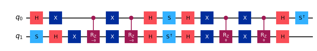
Figure 5: Elementary decomposition of the $1$-qubit convolution unitary $W_{\theta}^{(1)}$. Here $R_{z}(\theta)=\exp(-i\theta Z/2)$.

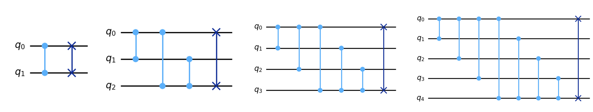
Figure 6: Swap gadget for $2,3,4,5$-qubit convolution unitaries. The blue and navy gates are $CZ$ and $\mathrm{SWAP}$, respectively. This gadget swaps the $2$ majorana operators associated with the top and botton lines while leaving others unchanged.

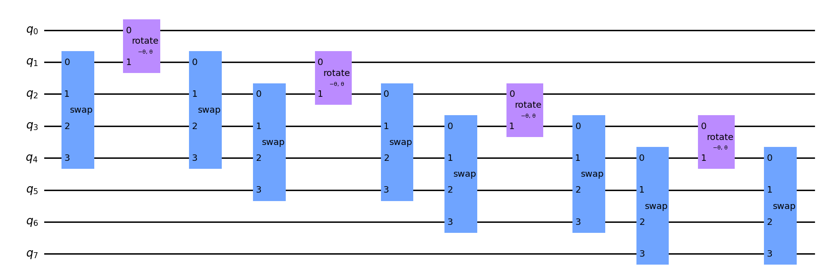
Figure 7: Elementary decomposition of the $4$-qubit convolution unitary. The purple “rotate” gadget is $W_{\theta}^{(1)}$ in Fig 5, while the blue “swap” gadget is expanded in Fig 6.

C.2 Properties of fermionic convolution

In this subsection, we prove several key properties of the fermionic convolution, inspired by results for classical convolution and discrete convolution [59, 60]. These properties support the validity of our convolution definition and highlight its relationship to both quantum and classical information theory. For the clarity, we first summarize the properties in the following lemma and leave the central limit theorem to Sec. D.

Lemma C.1 (Summary of properties).

For any even states $\rho,\sigma$ and Gaussian unitary $U_{G}$, fermionic convolution satisfies the following properties:

1. Commutativity (Corollary C.3): $\rho\boxtimes_{\pi/4}\sigma=\sigma\boxtimes_{\pi/4}\rho$.

2. Angle reflectivity (Corollary C.2): $\rho\boxtimes_{\theta}\sigma=\rho\boxtimes_{-\theta}\sigma$.

3. Commutativity with Gaussian unitaries (Proposition C.3): $U_{G}(\rho\boxtimes\sigma)U^{\dagger}_{G}=(U_{G}\rho U^{\dagger}_{G})\boxtimes(U_{G}\sigma U^{\dagger}_{G})$, for any Gaussian unitary $U_{G}$.

4. Convolution-multiplication duality (Theorem C.2): Let $\Xi_{\tau}\in\mathcal{G}_{2n}$ denote the Fourier transform of a quantum state $\tau\in\mathcal{C}_{2n}$, and let $\xi_{\alpha}:\mathcal{G}_{2n}\to\mathcal{G}_{2n}$ be the automorphism of the Grassmann algebra defined by $\xi_{\alpha}(\eta_{j})=\alpha\eta_{j}$, then

   $$\Xi_{\rho\boxtimes\sigma}=(\xi_{\cos\theta}\Xi_{\rho})(\xi_{\sin\theta}\Xi_{\sigma}).$$ (C.6)

5. Entropy inequality (Proposition C.6):

   $$S(\rho\boxtimes\sigma)\geq\frac{1}{2}S(\rho)+\frac{1}{2}S(\sigma).$$ (C.7)

   Equality holds if and only if $\rho=\sigma$ is equal to a Gaussian state.

6. Purity invariance implies normality (Corollary C.4): $\rho\boxtimes\rho$ is pure if and only if $\rho$ is a Gaussian state.

We begin by proving the convolution-multiplication duality, which will be helpful to prove other results. It was demonstrated for the special case $\theta=\pi/4$ and $\rho=\sigma$ in [54], Proposition 5.1. Here, we will provide a generalized proof, inspired by Hudson’s approach [54], and also a new and simple combinatorial proof. We first introduce the following operation on the algebras.

Definition C.1 (Contraction isomorphism).

Given a factor $\alpha\in\mathbb{C}$, the contraction isomorphism $\xi_{\alpha}:\mathcal{G}_{2n}\to\mathcal{G}_{2n}$ scales all generators by a scalar, i.e.,

$$\xi_{\alpha}\,\eta_{j}=\alpha\eta_{j},$$ (C.8)

The contraction can be extended to the whole algebra as

$$\xi_{\alpha}\eta_{A}=\alpha^{|A|}\eta_{A}.$$ (C.9)

Theorem C.2 (Convolution-multiplication duality).

For arbitrary $\rho$ and even state $\sigma$, the moment-generating operator under convolution satisfies the following relation

$$\Xi_{\rho\boxtimes_{\theta}\sigma} =(\xi_{\cos\theta}\Xi_{\rho})(\xi_{\sin\theta}\Xi_{\sigma}),$$ (C.10)

and the cumulant-generating operator under convolution satisfies the following relation

$$\Psi_{\rho\boxtimes_{\theta}\sigma}=\xi_{\cos\theta}\Psi_{\rho}+\xi_{\sin\theta}\Psi_{\sigma}.$$ (C.11)

Proof.

Equation (C.10) immediately implies (C.11) by taking logarithm. To prove (C.10), we only need to prove the following statement and extend by bilinearity:

$$\Xi_{\gamma_{J}\boxtimes_{\theta}\gamma_{K}}(\eta)=(\xi_{\cos\theta}\eta_{J})(\xi_{\sin\theta}\eta_{K}),$$ (C.12)

for all even $\gamma_{J},\gamma_{K}$. The right-hand side of C.12 equals

$$\cos^{|J|}\theta\sin^{|K|}\theta\prod_{a\in J}\eta_{a}\prod_{b\in K}\eta_{b},$$ (C.13)

is $0$ for $J\cap K\neq\emptyset$, and $\cos^{|J|}\theta\sin^{|K|}\theta\prod_{a\in J}\eta_{a}\prod_{b\in K}\eta_{b}$ for $J\cap K=\emptyset$ . The left-hand side of (C.12) equals

$$\gamma_{J}\boxtimes_{\theta}\gamma_{K}=\mathrm{Tr}_{2}\left[W_{\theta}(\gamma_{J}\otimes\gamma_{K})W_{\theta}^{\dagger}\right]=\mathrm{Tr}_{2}\left(W_{\theta}\gamma_{J}\gamma_{K}W_{\theta}^{\dagger}\right).$$ (C.14)

Applying equation (C.2) to the operator inside the trace yields

$$W_{\theta}\gamma_{J}\gamma_{K}W_{\theta}^{\dagger} =\prod_{a\in J}(\gamma_{j}\cos\theta-\gamma_{2n+j}\sin\theta)\cdot\prod_{b\in K}(\gamma_{k}\sin\theta+\gamma_{2n+k}\cos\theta).$$ (C.15)

Note that any component containing $\gamma_{2n+l}$ will be annihilated by $\mathrm{Tr}_{2}$. If $J\cap K=\emptyset$, the he only choice of factors in the expansion (C.15) is

$$\cos^{|J|}\sin^{|J|}\theta\prod_{a\in J}\gamma_{a}\prod_{b\in K}\gamma_{b}\implies\Xi_{\gamma_{J}\boxtimes_{\theta}\gamma_{K}}(\eta)=\cos^{|J|}\sin^{|J|}\theta\prod_{a\in J}\eta_{a}\prod_{b\in K}\eta_{b}.$$ (C.16)

If $J\cap K\neq\emptyset$, then

$$W_{\theta}\gamma_{J}\gamma_{K}W_{\theta}^{\dagger} =\pm(\gamma_{l}\cos\theta-\gamma_{2n+l}\sin\theta)(\gamma_{l}\sin\theta+\gamma_{2n+l}\cos\theta)(\cdots)$$ (C.17)

$$=\pm(\gamma_{l}^{2}\cos\theta\sin\theta-\gamma_{2n+l}^{2}\cos\theta\sin\theta+2(\cos^{2}\theta+\sin^{2}\theta)\gamma_{l}\gamma_{2n+l})(\cdots)$$

$$=\pm 2\gamma_{l}\gamma_{2n+l}(\cdots)$$

which is also $0$ after taking $\mathrm{Tr}_{2}$. This proves that the two sides of equation 
refeq:easyProofFormula are equal, completing the proof. ∎

We also provide another proof following Hudson’s method in [54], which may be of independent interest. To do so, we need an additional isomorphism.

Definition C.2 (Exchange isomorphism).

The exchange isomorphism $\mathcal{S}:\mathcal{C}_{2n}\otimes\mathcal{C}_{2n}\to\mathcal{C}_{2n}\otimes\mathcal{C}_{2n}$ is defined by

$$\mathcal{S}(\gamma_{j}\otimes 1)=1\otimes\gamma_{j},\quad\mathcal{S}(1\otimes\gamma_{j})=\gamma_{j}\otimes 1,$$ (C.18)

extended multiplicatively from generators to the whole algebra.

Proof.

Consider the space $\mathcal{C}_{2n}\otimes\mathcal{C}_{2n}\otimes_{f}\mathcal{G}_{2n}$, which we relabel as $\mathcal{C}_{1}\otimes\mathcal{C}_{2}\otimes_{f}\mathcal{G}$. Here $\mathcal{C}_{1}\otimes\mathcal{C}_{2}$ is the product space of $\rho\otimes\sigma$. Let $e^{F}\in\mathcal{C}_{2n}\otimes_{f}\mathcal{G}_{2n}$ denote the Fourier kernel. First expand the partial traces, note that $(\mathcal{S}\otimes_{f}1_{\mathcal{G}\to\mathcal{G}})\,(1_{\mathcal{C}_{1}}\otimes e^{F})$ effectively applies $K$ to the $\mathcal{C}_{1},\mathcal{G}$ components of $\mathcal{C}_{1}\otimes\mathcal{C}_{2}\otimes_{f}\mathcal{G}$.

$$\Xi_{\rho\boxtimes_{\theta}\sigma} =\mathrm{Tr}_{\mathcal{C}_{1}}[e^{F}(\rho\boxtimes\sigma)]=\mathrm{Tr}_{\mathcal{C}_{1}}\left[e^{F}\,\mathrm{Tr}_{\mathcal{C}_{2}}[W(\rho\otimes\sigma)W^{\dagger}]\right]$$ (C.19)

$$=\mathrm{Tr}_{\mathcal{C}_{1}\mathcal{C}_{2}}\left[[(\mathcal{S}\otimes_{f}1_{\mathcal{G}\to\mathcal{G}})\,(1_{\mathcal{C}_{1}}\otimes e^{F})](W\otimes_{f}1_{\mathcal{G}})(\rho\otimes\sigma\otimes_{f}1_{\mathcal{G}})(W^{\dagger}\otimes_{f}1_{\mathcal{G}})\right]$$

$$=\mathrm{Tr}_{\mathcal{C}_{1}\mathcal{C}_{2}}\left[(W^{\dagger}\otimes_{f}1_{\mathcal{G}})[(S\otimes_{f}1_{\mathcal{G}\to\mathcal{G}})\,(1_{\mathcal{C}_{1}}\otimes e^{F})](W\otimes_{f}1_{\mathcal{G}})(\rho\otimes\sigma\otimes_{f}1_{\mathcal{G}})\right].$$

Now consider $(W^{\dagger}\otimes_{f}1_{\mathcal{G}})[(\mathcal{S}\otimes_{f}1_{\mathcal{G}\to\mathcal{G}})\,(1_{\mathcal{C}_{1}}\otimes K)](W\otimes_{f}1_{\mathcal{G}})$. Recalling the Fourier kernel expansion (A.13), we have

$$(\mathcal{S}\otimes_{f}1_{\mathcal{G}\to\mathcal{G}})\,(1_{\mathcal{C}_{1}}\otimes e^{F}) =\sum_{J}(\mathcal{S}\otimes_{f}1_{\mathcal{G}\to\mathcal{G}})\,[(1_{\mathcal{C}_{1}}\otimes 1_{\mathcal{C}_{2}}\otimes_{f}\eta_{J})(1_{\mathcal{C}_{1}}\otimes\gamma_{J}^{\dagger}\otimes_{f}1_{\mathcal{G}})]$$

$$=\sum_{J}(1_{\mathcal{C}_{1}}\otimes 1_{\mathcal{C}_{2}}\otimes_{f}\eta_{J})(\gamma_{J}^{\dagger}\otimes 1_{\mathcal{C}_{2}}\otimes_{f}1_{\mathcal{G}})$$

$$=\exp\left[\sum_{j}(\gamma_{j}\otimes 1_{\mathcal{C}_{2}}\otimes_{f}1_{\mathcal{G}})(1_{\mathcal{C}_{1}}\otimes 1_{\mathcal{C}_{2}}\otimes_{f}\eta_{j})\right].$$

Unitary conjugation by $W^{\dagger}\otimes 1_{\mathcal{G}}$ acts on the exponent of the expression above as follows

$$(W^{\dagger}\otimes 1_{\mathcal{G}})\left[(\gamma_{j}\otimes 1_{\mathcal{C}_{2}}\otimes_{f}1_{\mathcal{G}})(1_{\mathcal{C}_{1}}\otimes 1_{\mathcal{C}_{2}}\otimes_{f}\eta_{j})\right](W\otimes 1_{\mathcal{G}})$$

$$=\left[(W^{\dagger}\otimes 1_{\mathcal{G}})(\gamma_{j}\otimes 1_{\mathcal{C}_{2}}\otimes_{f}1_{\mathcal{G}})(W\otimes 1_{\mathcal{G}})\right](1_{\mathcal{C}_{1}}\otimes 1_{\mathcal{C}_{2}}\otimes_{f}\eta_{j})$$

$$=\left[\cos\theta(\gamma_{j}\otimes 1_{\mathcal{C}_{2}}\otimes_{f}1_{\mathcal{G}})+\sin\theta(Z^{\otimes n}\otimes\gamma_{j}\otimes_{f}1_{\mathcal{G}})\right](1_{\mathcal{C}_{1}}\otimes 1_{\mathcal{C}_{2}}\otimes_{f}\eta_{j}).$$

This yields conjugate action on $[(\mathcal{S}\otimes_{f}1_{\mathcal{G}\to\mathcal{G}})\,(1_{\mathcal{C}_{1}}\otimes K)]$

$$(W^{\dagger}\otimes_{f}1_{\mathcal{G}})[(\mathcal{S}\otimes_{f}1_{\mathcal{G}\to\mathcal{G}})\,(1_{\mathcal{C}_{1}}\otimes K)](W\otimes_{f}1_{\mathcal{G}})$$ (C.20)

$$= \exp\left[\sum_{j}\left[\cos\theta(\gamma_{j}\otimes 1_{\mathcal{C}_{2}}\otimes_{f}1_{\mathcal{G}})+\sin\theta(Z^{\otimes n}\otimes\gamma_{j}\otimes_{f}1_{\mathcal{G}})\right](1_{\mathcal{C}_{1}}\otimes 1_{\mathcal{C}_{2}}\otimes_{f}\eta_{j})\right].$$

Note that $Z^{\otimes n}\otimes\gamma_{j}^{(2n)}\cong\gamma_{2n+j}^{(4n)}$. Here, to simplify the notation, we used the Jordan-Wigner representation $Z^{\otimes n}$ to denote its algebraic equivalent. Since $\sigma$ is even, in the power expansion of the exponential, only terms that are even in $\mathcal{C}_{2}$ contribute nontrivially after $\mathrm{Tr}_{\mathcal{C}_{1}\mathcal{C}_{2}}$ in equation (C.19). More precisely, let $\Phi:\mathcal{C}_{1}\otimes\mathcal{C}_{2}\otimes_{f}\mathcal{G}\to\mathcal{C}_{1}\otimes\mathcal{C}_{2}\otimes_{f}\mathcal{G}$ be the projection operator onto the even subspace of $\mathcal{C}_{2}$ so that $\Phi(\gamma_{J}\otimes\gamma_{K}\otimes_{f}\eta_{L})=\gamma_{J}\otimes\gamma_{K}\otimes_{f}\eta_{L}$ iff $\gamma_{K}\in\mathcal{C}_{2}$ is even else $0$, then

$$\Xi_{\rho\boxtimes_{\theta}\sigma} =\mathrm{Tr}_{\mathcal{C}_{1}\mathcal{C}_{2}}\left[(W^{\dagger}\otimes_{f}1_{\mathcal{G}})[(S\otimes_{f}1_{\mathcal{G}\to\mathcal{G}})\,(1_{\mathcal{C}_{1}}\otimes e^{F})](W\otimes_{f}1_{\mathcal{G}})(\rho\otimes\sigma\otimes_{f}1_{\mathcal{G}})\right]$$ (C.21)

$$=\mathrm{Tr}_{\mathcal{C}_{1}\mathcal{C}_{2}}\left[\Phi\left[(W^{\dagger}\otimes_{f}1_{\mathcal{G}})[(S\otimes_{f}1_{\mathcal{G}\to\mathcal{G}})\,(1_{\mathcal{C}_{1}}\otimes e^{F})](W\otimes_{f}1_{\mathcal{G}})\right](\rho\otimes\sigma\otimes_{f}1_{\mathcal{G}})\right].$$

The even-parity projection of (LABEL:eq:FourierExponent) in the expression above gets rid of the $Z^{\otimes n}$ factor, yielding

$$\Phi(\ref{eq:FourierExponent}) =\exp\left[\sum_{j}\left[\cos\theta(\gamma_{j}\otimes 1_{\mathcal{C}_{2}}\otimes_{f}1_{\mathcal{G}})+\sin\theta(1_{\mathcal{C}_{1}}\otimes\gamma_{j}\otimes_{f}1_{\mathcal{G}})\right](1_{\mathcal{C}_{1}}\otimes 1_{\mathcal{C}_{2}}\otimes_{f}\eta_{j})\right]$$

$$=\exp\left[\sum_{j}(\gamma_{j}\otimes 1_{\mathcal{C}_{2}}\otimes_{f}1_{\mathcal{G}})(1_{\mathcal{C}_{1}}\otimes 1_{\mathcal{C}_{2}}\otimes_{f}(\cos\theta\cdot\eta_{j}))\right]\exp\left[\sum_{j}(1_{\mathcal{C}_{1}}\otimes\gamma_{j}\otimes_{f}1_{\mathcal{G}})(1_{\mathcal{C}_{1}}\otimes 1_{\mathcal{C}_{2}}\otimes_{f}(\sin\theta\cdot\eta_{j}))\right]$$

$$=(\xi_{\cos\theta}e^{F_{1}})(\xi_{\sin\theta}e^{F_{2}}).$$

Here $e^{F_{1}},e^{F_{2}}$ are the Fourier kernels defined on $(\mathcal{C}_{1},\mathcal{G})$ and $(\mathcal{C}_{2},\mathcal{G})$ and extended trivially,

$$e^{F_{1}} =\exp\left[\sum_{j}(\gamma_{j}\otimes 1_{\mathcal{C}_{2}}\otimes_{f}1_{\mathcal{G}})(1_{\mathcal{C}_{1}}\otimes 1_{\mathcal{C}_{2}}\otimes_{f}\eta_{j})\right]\in\mathcal{C}_{1}\otimes\mathcal{C}_{2}\otimes_{f}\mathcal{G}$$

$$e^{F_{1}} =\exp\left[\sum_{j}(1_{\mathcal{C}_{1}}\otimes\gamma_{j}\otimes 1_{\mathcal{G}})(1_{\mathcal{C}_{1}}\otimes 1_{\mathcal{C}_{2}}\otimes_{f}\eta_{j}\right]\in\mathcal{C}_{1}\otimes\mathcal{C}_{2}\otimes_{f}\mathcal{G}.$$

Then substituting $\Phi(\ref{eq:FourierExponent})=(\xi_{\cos\theta}e^{F_{1}})(\xi_{\sin\theta}e^{F_{2}})$ into equation (C.21) yields

$$\Xi_{\rho\boxtimes\sigma} =\mathrm{Tr}_{\mathcal{C}_{1}\mathcal{C}_{2}}\left[\Phi\left[(W^{\dagger}\otimes_{f}1_{\mathcal{G}})[(S\otimes_{f}1_{\mathcal{G}\to\mathcal{G}})\,(1_{\mathcal{C}_{1}}\otimes e^{F})](W\otimes_{f}1_{\mathcal{G}})\right](\rho\otimes\sigma\otimes_{f}1_{\mathcal{G}})\right]$$

$$=\mathrm{Tr}_{\mathcal{C}_{1}\mathcal{C}_{2}}\left[(\xi_{\cos\theta}e^{F_{1}})(\xi_{\sin\theta}e^{F_{2}})(\rho\otimes\sigma\otimes_{f}1_{\mathcal{G}})\right]$$

$$=\mathrm{Tr}_{\mathcal{C}_{1}\mathcal{C}_{2}}\left[[(\xi_{\cos\theta}e^{F_{1}})(\rho\otimes 1_{\mathcal{C}_{2}}\otimes_{f}1_{\mathcal{G}})][(\xi_{\sin\theta}e^{F_{2}})(1_{\mathcal{C}_{1}}\otimes\sigma\otimes_{f}1_{\mathcal{G}})]\right]$$

$$=\mathrm{Tr}_{\mathcal{C}}[(\xi_{\cos\theta}e^{F})(\rho\otimes_{f}1_{\mathcal{G}})]\cdot\mathrm{Tr}_{\mathcal{C}}[(\xi_{\sin\theta}K)(\sigma\otimes_{f}1_{\mathcal{G}})]=(\xi_{\cos\theta}\Xi_{\rho})(\xi_{\sin\theta}\Xi_{\sigma}).$$

∎

According to (C.11) , the components of the cumulants under the convolution satisfies the following relation,

$$\kappa^{\rho\boxtimes_{\theta}\sigma}_{J}=\kappa^{\rho}_{J}\cos^{j}\theta+\kappa^{\sigma}_{J}\sin^{j}\theta.$$ (C.22)

That is, the quadratic cumulants are preserved, while the higher-order cumulants shrink.

Corollary C.1 (Fixed points of convolution).

For any Gaussian state $\rho_{G}$, $\rho_{G}\boxtimes_{\theta}\rho_{G}=\rho_{G}$.

Corollary C.2 (Angle-reflectivity).

For any even states $\rho$ and $\sigma$, we have $\rho\boxtimes_{\theta}\sigma=\rho\boxtimes_{-\theta}\sigma$ for all $\theta$.

Proof.

Note that any even state is determined by the cumulant. It is easy to see that the equation C.22 is invariant under $\theta\mapsto-\theta$ for even $\rho,\sigma$, hence $\rho\boxtimes_{\theta}\sigma=\rho\boxtimes_{-\theta}\sigma$ .

∎

Corollary C.3 (Commutativity).

For any even states $\rho$ and $\sigma$, we have $\rho\boxtimes_{\theta}\sigma=\sigma\boxtimes_{\theta}\rho$ when $\cos\theta=\sin\theta$.

Proof.

Based on the equation (C.22), the invariance is also preserved under reflection of $\rho$ and $\sigma$ when $\cos\theta=\sin\theta$. ∎

Proposition C.3 (Commutativity with Gaussian unitaries).

For any Gaussian unitary $U_{G}$, we have

$$U_{G}(\rho\boxtimes\sigma)U^{\dagger}_{G}=(U_{G}\rho U^{\dagger}_{G})\boxtimes(U_{G}\sigma U^{\dagger}_{G}).$$ (C.23)

Proof.

We only need to prove that $\Xi_{U_{G}(\rho\boxtimes\sigma)U^{\dagger}_{G}}=\Xi_{(U_{G}\rho U^{\dagger}_{G})\boxtimes(U_{G}\sigma U^{\dagger}_{G})}$. Since the conjugate action of the Gaussian unitary $U_{G}$ corresponds to a rotation $R$ as in (A.15), then left-hand side can be written as

$$\Xi_{U_{G}(\rho\boxtimes\sigma)U^{\dagger}_{G}}(\eta)=\Xi_{\rho\boxtimes\sigma}(R\eta)=\Xi_{\rho}(R\eta)\Xi_{\sigma}(R\eta).$$

Apply the convolution-multiplication duality, the right-hand side can be

$$\Xi_{\rho}(R\eta)\Xi_{\sigma}(R\eta)=\Xi_{U_{G}\rho U^{\dagger}_{G}}(\eta)\Xi_{U_{G}\sigma U^{\dagger}_{G}}(\eta)=\Xi_{(U_{G}\rho U^{\dagger}_{G})\boxtimes(U_{G}\sigma U^{\dagger}_{G})}(\eta).$$

The Fourier transforms are equal iff the states are equal, completing the proof. ∎

Lemma C.4 (Angle-reflection$+$exchange symmetry of the convolution unitary).

For all even basis elements $\gamma_{J},\gamma_{K}$,

$$\mathcal{S}[W_{\theta}(\gamma_{J}\otimes\gamma_{K})W_{\theta}^{\dagger}]=W_{-\theta}(\gamma_{K}\otimes\gamma_{J})W_{-\theta}^{\dagger}.$$ (C.24)

Proof.

Let $\varphi_{\theta}:\mathcal{C}_{2n}\otimes\mathcal{C}_{2n}\to\mathcal{C}_{2n}\otimes\mathcal{C}_{2n}$ denote the isomorphism $\varphi_{\theta}(A)=W_{\theta}AW_{\theta}^{\dagger}$, then (C.24) claims $\mathcal{S}\circ\varphi_{\theta}=\varphi_{-\theta}$ on the even subspace of $\mathcal{C}_{2n}\otimes\mathcal{C}_{2n}$. To see this, recall that Definition (II.2),

$$\varphi_{\theta}(\gamma_{j})=\cos\theta\gamma_{j}-\sin\theta\gamma_{2n+j},$$

$$\varphi_{\theta}(\gamma_{2n+j})=\sin\theta\gamma_{j}+\cos\theta\gamma_{2n+j},$$

is invariant under $\theta\mapsto-\theta,\gamma_{j}\leftrightarrow\gamma_{2n+j}$, where $\gamma_{j}\leftrightarrow\gamma_{2n+j}$ is exactly the action of $\mathcal{S}$ on $\mathcal{C}_{2n}\otimes\mathcal{C}_{2n}$ for even elements. ∎

Lemma C.5.

For any even states $\rho,\sigma$, let $\rho\,{\tilde{\boxtimes}_{\theta}}\,\sigma:=\mathrm{Tr}_{1}\left[W_{\theta}(\rho\otimes\sigma)W_{\theta}^{\dagger}\right]$ be the complementary channel, we have

$$\rho\,{\tilde{\boxtimes}_{\theta}}\,\sigma=\rho\boxtimes_{\theta}\sigma.$$ (C.25)

Proof.

$\rho\,{\tilde{\boxtimes}_{-\theta}}\,\sigma=\mathrm{Tr}_{1}\left[W_{\theta}(\rho\otimes\sigma)W_{\theta}^{\dagger}\right]=\mathrm{Tr}_{1}\left[\varphi_{\theta}(\rho\otimes\sigma)\right]=\mathrm{Tr}_{2}\left[(\mathcal{S}\circ\varphi_{\theta})(\rho\otimes\sigma)\right]=\mathrm{Tr}_{2}\left[\varphi_{-\theta}(\rho\otimes\sigma)\right]=\rho\boxtimes_{-\theta}\sigma$. ∎

Proposition C.6 (Entropy inequality under fermionic convolution).

Given two even states $\rho$ and $\sigma$, we have

$$S(\rho\boxtimes_{\theta}\sigma)\geq\frac{1}{2}S(\rho)+\frac{1}{2}S(\sigma),$$ (C.26)

equality holds iff $\rho=\sigma$ is a Gaussian state.

Proof.

Recall that $\rho\boxtimes_{\theta}\sigma$, $\rho\,{\tilde{\boxtimes}}_{\theta}\,\sigma$ are the two reduced states of $\tau_{ab}=W(\rho\otimes\sigma)W^{\dagger}$, then by the subadditivity of quantum entropy and Lemma C.5,

$$S(\rho)+S(\sigma)=S(\tau_{AB})\leq S(\rho\boxtimes_{\theta}\sigma)+S(\rho\,\tilde{\boxtimes}_{\theta}\,\sigma)=2S(\rho\boxtimes_{\theta}\sigma).$$ (C.27)

Equality holds iff subadditivity is saturated, which means

$$W(\rho\otimes\sigma)W^{\dagger}=(\rho\boxtimes_{\theta}\sigma)\otimes(\rho\,\tilde{\boxtimes}_{\theta}\,\sigma).$$

This is also equivalent to

$$\rho\otimes\sigma=W^{\dagger}[(\rho\boxtimes_{\theta}\sigma)\otimes(\rho\boxtimes_{\theta}\sigma)]W.$$ (C.28)

By taking the two reduced states of the right hand side, which are equal to $\rho$ and $\sigma$ respectively. Thus,

$$\rho=(\rho\boxtimes_{\theta}\sigma)\boxtimes(\rho\boxtimes_{\theta}\sigma)=(\rho\boxtimes_{\theta}\sigma)\,\tilde{\boxtimes}_{\theta}\,(\rho\boxtimes_{\theta}\sigma)=\sigma.$$ (C.29)

Moreover, by applying the previous argument iteratively and the central limit theorem for fermionic convolution in Proposition D.1, we have

$$\rho=(\rho\boxtimes_{\theta}\rho)\boxtimes_{\theta}(\rho\boxtimes_{\theta}\rho)=...=\mathcal{G}(\rho).$$ (C.30)

Therefore, $\rho=\sigma$ is a fermionic Gaussian state. ∎

One direct implication of the entropy inequality is the monotonicity of quantum entropy under fermionic convolution. This principle is analogous to the second law of thermodynamics in the context of fermionic convolution.

Proposition C.7.

For any even state $\rho$, we have

$$S(\boxtimes^{k+1}\rho)\geq S(\boxtimes^{k}\rho),\forall k.$$ (C.31)

Corollary C.4 (Purity invariance implies normality).

$\rho\boxtimes\rho$ is pure if and only if $\rho$ is a pure Gaussian state.

Proof.

If $\rho$ is pure Gaussian, then $\rho\boxtimes\rho=\rho$ is pure by Corollary C.1. The converse implies $S(\rho)=0$ and the saturation condition of the entropy inequality $\rho=\mathcal{G}(\rho)$. ∎

Proposition C.8 (Gaussian characterization by maximum entropy).

Let $M$ be a real and antisymmetric $2n\times 2n$ matrix with $M^{T}M\leq I$, and $\mathcal{Q}(M)$ be the set of all even $n$-qubit quantum states with covariance matrix $M$, then the unique Gaussian state $\rho_{G}\in\mathcal{Q}(M)$ has maximum entropy.

Proof.

The Gaussian $\rho_{G}\in\mathcal{Q}(M)$ is unique since Gaussian states are specified by their covariance matrix. Moreover, since covariance matrix is preserved under convolution, i.e., $\Sigma_{\rho\boxtimes\rho}=\Sigma_{\rho}$, then $\rho\boxtimes\rho$ is also in $\mathcal{Q}(M)$ for any $\rho\in\mathcal{Q}(M)$. Let $\rho_{0}=\mathrm{argmax}_{\rho\in\mathcal{Q}(M)}S(\rho)$, then $S(\rho_{0}\boxtimes\rho_{0})=S(\rho_{0})$. By the entropy inequality in Proposition C.6, we have that $\rho_{0}$ is a Gaussian state. ∎

Proposition C.9 (Gaussian characterization by maximum Gaussian weight).

Given $0\leq S_{0}\leq n\log 2$, define

$$\mathcal{R}(S_{0})=\{n\text{-qubit state }\rho:\rho\text{ even and }S(\rho)=S_{0}\}.$$ (C.32)

If $\rho\in\mathcal{R}(S_{0})$ has maximum Gaussian weight $K_{G}$, then is Gaussian.

Proof.

For the sake of contradiction, suppose that a non-Gaussian state $\rho\in\mathcal{R}(S_{0})$ has maximum Gaussian weight $K_{G}$, then $S(\mathcal{G}(\rho))>S(\rho)$. Then applying Lemma B.6 to $\mathcal{G}(\rho)$ with $S_{0}=S(\rho)$ implies the existence of a Gaussian state $\sigma$ satisfying $S(\sigma)=S_{0}<S(\rho)$ and $K_{G}(\sigma)>K_{G}(\rho)$. ∎

Applying this to the extremal case $S_{0}=0$, we obtain the Gaussian-weight characterization of pure Gaussian states.

Corollary C.5.

A $n$-qubit even state $\psi$ is Gaussian if and only if $K_{G}(\psi)=n$.

C.3 Properties of non-Gaussian entropy and its generalization to Rényi entropy

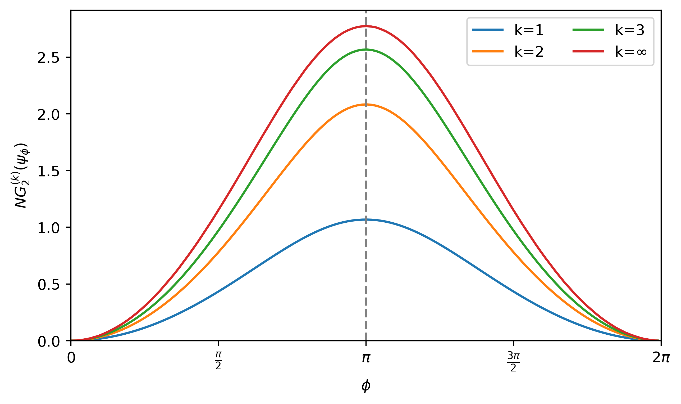
Figure 8: Non-Gaussian Rényi entropy $NG^{(k)}_{2}$ of the 4-qubit parametrized state $\psi_{\phi}$ in  (B.34).

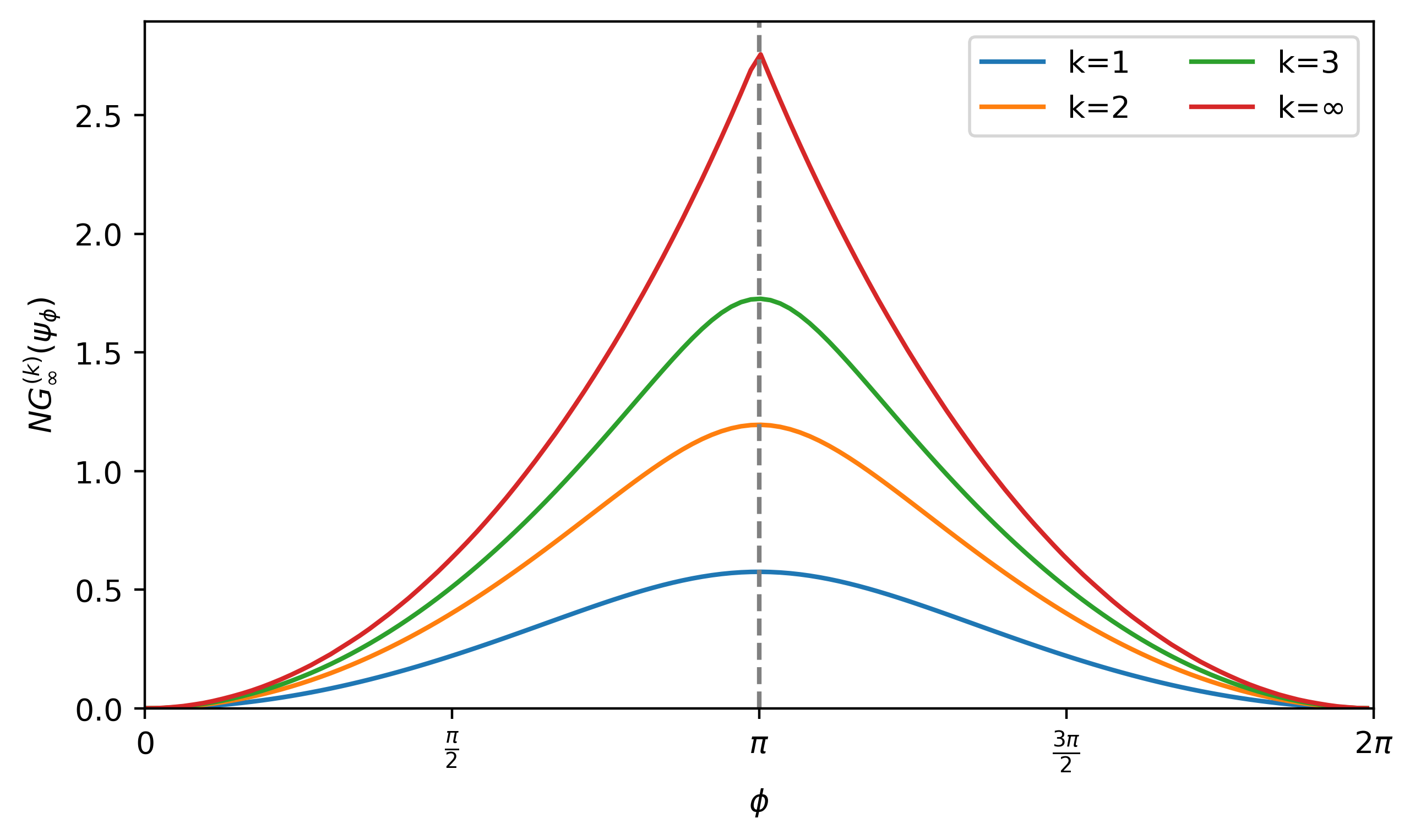
Figure 9: Non-Gaussian Rényi entropy $NG^{(k)}_{\infty}$of the 4-qubit parametrized state $\psi_{\phi}$ in  (B.34).

Recall that the non-Gaussian entropy is defined as

$$NG(\psi)=S(\psi\boxtimes\psi).$$ (C.33)

Proposition C.10 (Restatement of Theorem 7).

The Non-Gaussian entropy $NG(\psi)$ for even pure state $\psi$ satisfies the following properties:

1. Faithfiulness: $NG(\psi)\geq 0$ with equality iff $\psi$ is a fermionic Gaussian.

2. Gaussian invariance: $NG(U_{G}\left|\psi\right\rangle\!\left\langle\psi\right|U^{\dagger}_{G})=NG(\left|\psi\right\rangle\!\left\langle\psi\right|)$ for any Gaussian unitary $U_{G}$.

3. Additivity under tensor product: $NG(\psi_{1}\otimes\psi_{2})=NG(\psi_{1})+NG(\psi_{2})$.

Proof.

(1) $NG(\psi)\geq 0$ follows from definition with equality iff $S(\psi\boxtimes\psi)=S(\psi)$. By the saturation condition of the entropy inequality in Proposition C.6, we have $NG(\psi)=0$ iff $\psi$ is a fermionic Gaussian.

(2) Gaussian unitary-invariance follows from convolution commuting with Gaussian unitary in Proposition C.3.

(3) $NG$-additivity follows from $(\psi_{1}\otimes\psi_{2})\boxtimes(\psi_{1}\otimes\psi_{2})=(\psi_{1}\boxtimes\psi_{2})\otimes(\psi_{1}\boxtimes\psi_{2})$.

∎

Consider the extension of non-Gaussian entropy to higher-order, Rényi non-Gaussian entropy as follows

$$NG^{(k)}_{\alpha}(\psi)=S_{\alpha}(\boxtimes^{k}\psi),$$ (C.34)

where the $\alpha$-Rényi entropy $S_{\alpha}$ with $\alpha\in[0,+\infty]$ is defined as

$$S_{\alpha}(\rho)=\frac{1}{1-\alpha}\operatorname{Tr}\left[\rho^{\alpha}\right].$$ (C.35)

The Rényi generalization $NG^{(k)}_{\alpha}$ also satisfies the essential properties of faithfulness, Gaussian invariance, and additivity under tensor product, making it a valuable measure for quantifying fermionic non-Gaussianity.

Let us again consider the $4$-qubit parametrized state $\psi_{\phi}$ in  (B.34), $\ket{\psi_{\phi}}=\frac{1}{2}\left(\ket{0000}+\ket{0011}+\ket{1100}+e^{i\phi}\ket{1111}\right)$, with $\phi\in[0,2\pi]$. This degenerates to the von-Neumann definition (Fig 2) with $\alpha=1$. The $\alpha=2,\infty$ cases are shown in Fig 9 and 9. When $\alpha=0$, for all $k>0$ we have

$$NG^{(k)}_{0}(\psi_{\phi})=\begin{cases}0,&\phi\in\{0,2\pi\},\\ 4\log 2,&\text{otherwise.}\end{cases}$$ (C.36)

Appendix D Central limit theorem and convergence rate

This section derives the central limit for fermionic convolution and provides a bound on its rate of convergence. Let us define the $k$-th iteration of self-convolution

$$\boxtimes^{k+1}_{\theta}\rho=(\boxtimes^{k}\rho)\boxtimes_{\theta}(\boxtimes^{k}\rho),\quad\text{with}~{}\quad\boxtimes^{0}\rho=\rho.$$ (D.1)

Proposition D.1 (Central limit theorem).

For any even state $\rho$, we have

$$\lim_{k\to\infty}\boxtimes^{k}_{\theta}\rho=\mathcal{G}(\rho).$$ (D.2)

Proof.

We prove for $\theta=\pi/4$, general case follows easily. A even state is Gaussian if and only if it has vanishing super-quadratic cumulants, i.e., $\kappa_{J}=0$ for any $J$ with $|J|\geq 4$. The convolution-multiplication duality C.11 implies

$$\kappa^{\rho\boxtimes_{\theta}\rho}_{J}=\kappa^{\rho}_{J}\cos^{j}\theta+\kappa^{\rho}_{J}\sin^{j}\theta.$$

This yields the following equation for $j$-th order cumulants

$$\kappa^{\boxtimes^{k+1}\rho}_{J} =2\left(\dfrac{1}{\sqrt{2}}\right)^{j}\kappa^{\boxtimes^{k}\rho}_{J}=2^{k(1-j/2)}\kappa^{\rho}_{J}.$$ (D.3)

Note that $j=|J|$ is always even. Therefore,

$$\lim_{k\to\infty}2^{k(1-j/2)}\kappa^{\rho}_{J}=\begin{cases}\kappa^{\rho}_{J}&j=2,\\ 0&\text{otherwise}.\end{cases}$$

These are exactly the cumulants of $\mathcal{G}(\rho)$. ∎

Next, we study the convergence rate of the central limit theorem (CLT). We prove results for $\theta=\pi/4$, and the approach can be readily extended to more general cases.

Lemma D.2.

For any linear operators $X,Y$, we have

$$\|e^{X+Y}-e^{X}\|\leq\|Y\|e^{\|X\|+\|Y\|},$$

where $\|A\|=\sup_{\|\vec{x}\|\leq 1}\|A\vec{x}\|$ denotes the operator norm.

Proof.

Denote $x=\|X\|,y=\|Y\|$. Expand the series and use submultiplicativity and subadditivity:

$$\|e^{X+Y}-e^{X}\| \leq\sum_{n=0}^{\infty}\dfrac{1}{n!}\|(X+Y)^{n}-X^{n}\|$$

$$\leq\sum_{n=0}^{\infty}\dfrac{1}{n!}\sum_{k=0}^{\infty}\binom{n}{k}x^{k}y^{n-k}-x^{n}$$

$$=\sum_{n=0}^{\infty}\dfrac{1}{n!}\sum_{k=0}^{n-1}\binom{n}{k}x^{k}y^{n-k}$$

$$=\sum_{n=0}^{\infty}\dfrac{1}{n!}\sum_{k=0}^{n-1}\binom{n-1}{k-1}x^{k}y^{n-k}+\sum_{k=0}^{n-1}\binom{n-1}{k}x^{k}y^{n-k}.$$

Let us consider the first term in the sum, substitute $k\mapsto k+1$ and factor out an $x$

$$\sum_{k=0}^{n-1}\binom{n-1}{k-1}x^{k}y^{n-k}=x\sum_{k=0}^{n-2}\binom{n-1}{k}x^{k}y^{(n-1)-k}=x[(x+y)^{n-1}-x^{n-1}]=x(x+y)^{n-1}-x^{n}.$$

The second term is defined similarly

$$\sum_{k=0}^{n-1}\binom{n-1}{k}x^{k}y^{n-k}=y(x+y)^{n-1}.$$

Substitute back into the expression, which now simplifies neatly

$$\|e^{X+Y}-e^{X}\|\leq\sum_{n=0}^{\infty}\dfrac{(x+y)^{n}-x^{n}}{n!}=e^{x+y}-e^{x}=e^{x}(e^{y}-1)\leq ye^{x}e^{y}.$$

∎

Lemma D.3.

Let for $n$-qubit states $\rho,\sigma$, we have

$$\|\rho-\sigma\|_{2}=\dfrac{1}{2^{n}}\|\Xi_{\rho}-\Xi_{\sigma}\|_{2}\leq\|\Xi_{\rho}-\Xi_{\sigma}\|,$$

where $\|\cdot\|_{2}$ denotes the $L_{2}$-norm,

Proof.

This equation comes from the fact that $L_{2}$ norm is preserved under the Grassmann-Clifford Fourier transform. The inequality comes from the bound on the operator norm by the $L_{2}$ norm. ∎

Theorem D.4 (Convergence rate of central limit theorem).

For a $n$-qubit even state $\rho$

$$\|\boxtimes^{k}\rho-\mathcal{G}(\rho)\|_{2} \leq\dfrac{\sqrt{K_{M}(\rho)}}{2^{k}}\exp\left(\sqrt{K_{G}(\rho)}+2^{-k}\sqrt{K_{M}(\rho)}\right),$$ (D.4)

where $K_{G}$ and $K_{M}$ denote the Gaussian and non-Gaussian weights in definition B.5.

Proof.

Recall the cumulant-generating operator under the convolution is equal to

$$\Psi_{\boxtimes^{k}\rho}=\sum_{J}2^{-k(j/2-1)}\kappa^{\rho}_{J}\eta_{J},$$

while the limit state $\mathcal{G}(\rho)$ has the following form

$$\Psi_{\mathcal{G}(\rho)}=\sum_{|J|=2}\kappa^{\rho}_{J}\eta_{J}.$$

The operator norm of $\Psi_{\boxtimes^{k}\rho}-\Psi_{\mathcal{G}(\rho)}$ is bounded by the $L_{2}$ norm

$$\|\Psi_{\boxtimes^{k}\rho}-\Psi_{\mathcal{G}(\rho)}\|\leq\|\Psi_{\boxtimes^{k}\rho}-\Psi_{\mathcal{G}(\rho)}\|_{2}=\sqrt{\sum_{|J|>2}|2^{-k(|J|/2-1)}\kappa_{J}|^{2}}\leq 2^{-k}\sqrt{K_{M}(\rho)}.$$

By using Lemma D.3 and substituting $X\mapsto\Psi_{\mathcal{G}(\rho)},Y\mapsto\Psi_{\boxtimes^{k}\rho}-\Psi_{\mathcal{G}(\rho)}$:

$$\|\boxtimes^{k}\rho-\mathcal{G}(\rho)\|_{2}\leq\|\Xi_{\boxtimes^{k}\rho}-\Xi_{\mathcal{G}(\rho)}\|=\|\exp\Psi_{\boxtimes^{k}\rho}-\exp\Psi_{\mathcal{G}(\rho)}\|=\|e^{X+Y}-e^{X}\|.$$

Invoke lemma D.2 to obtain the desired bound:

$$\|\boxtimes^{k}\rho-\mathcal{G}(\rho)\|_{2}\leq\|e^{X+Y}-e^{X}\|\leq ye^{x+y}=\dfrac{\sqrt{K_{M}(\rho)}}{2^{k}}\exp\left(\sqrt{K_{G}(\rho)}+2^{-k}\sqrt{K_{M}(\rho)}\right).$$

where the relevant quantities $y=\|Y\|,x=\|X\|$ are

$$x=\|\Psi_{\mathcal{G}(\rho)}\|\leq\|\Psi_{\mathcal{G}(\rho)}\|_{2}=\sqrt{K_{G}(\rho)},\quad y=\|\Psi_{\boxtimes^{k}\rho}-\Psi_{\mathcal{G}(\rho)}\|\leq 2^{-k}\sqrt{K_{M}(\rho)}.$$

∎

One may also consider a version of the central limit theorem which consumes an arbitrary positive integer $n$ instead of $2^{k}$ number of copies of the state $\rho$. For each $m>0$, define the convolution angle $\theta_{m}\in(0,\pi/2)$ which satisfies

$$\cos^{2}\theta_{m}=\dfrac{m}{m+1}.$$ (D.5)

Consider the version of iterated convolution linear in the number of copies so that $\boxtimes^{k}\rho$ requires $k$ copies of $\rho$

$$\boxtimes^{(1)}\rho=\rho,\quad\boxtimes^{(k+1)}\rho=(\boxtimes^{(k)}\rho)\boxtimes_{\theta_{k}}\rho.$$ (D.6)

In particular, $\boxtimes^{(2)}\rho=\rho\boxtimes_{\pi/4}\rho,\,\,\boxtimes^{(3)}\rho=(\rho\boxtimes_{\pi/4}\rho)\boxtimes_{\theta_{2}}\rho$, etc. We now compute the cumulants of iterated convolution by applying additivity (C.22). Let us first consider the quadratic case

$$\kappa^{\boxtimes^{(n)}\rho}_{J} =\kappa^{\rho}_{J}\sin^{2}\theta_{n}+\kappa^{\boxtimes^{(n-1)}\rho}_{J}\cos^{2}\theta_{n}=\frac{1}{n}\kappa^{\rho}_{J}+\dfrac{n-1}{n}\kappa^{\boxtimes^{(n-1)}\rho}_{J}$$ (D.7)

$$=\frac{1}{n}\kappa^{\rho}_{J}+\dfrac{n-1}{n}\left(\frac{1}{n-1}\kappa^{\rho}_{J}+\frac{n-1}{n-2}\kappa^{\boxtimes^{(n-2)}\rho}_{J}\right)$$

$$=\cdots=\kappa^{\rho}_{J},\quad\text{where}~{}|J|=2.$$

In general, for the cumulant with $|J|=2m$, we have

$$\kappa^{\boxtimes^{(n)}\rho}_{J} =\kappa^{\rho}_{J}\sin^{2m}\theta_{n}+\kappa^{\boxtimes^{(n-1)}\rho}_{J}\cos^{2m}\theta_{n}=\frac{1}{n^{m}}\kappa^{\rho}_{J}+\left(\dfrac{n-1}{n}\right)^{m}\kappa^{\boxtimes^{(n-1)}\rho}_{J}$$ (D.8)

$$=\frac{1}{n^{m}}\kappa^{\rho}_{J}+\left(\dfrac{n-1}{n}\right)^{m}\left[\frac{1}{(n-1)^{m}}\kappa^{\rho}_{J}+\left(\dfrac{n-2}{n-1}\right)^{m}\kappa^{\boxtimes^{(n-2)}\rho}_{J}\right]$$

$$=\frac{1}{n^{m}}\kappa^{\rho}_{J}+\dfrac{1}{n^{m}}\kappa^{\rho}_{J}+\left(\dfrac{n-2}{n}\right)^{m}\kappa^{\boxtimes^{(n-2)}\rho}_{J}$$

$$=\frac{1}{n^{m}}\kappa^{\rho}_{J}+\dfrac{1}{n^{m}}\kappa^{\rho}_{J}+\left(\dfrac{n-2}{n}\right)^{m}\left[\frac{1}{(n-2)^{m}}\kappa^{\rho}_{J}+\left(\dfrac{n-3}{n-2}\right)^{m}\kappa^{\boxtimes^{(n-3)}\rho}_{J}\right]$$

$$=\frac{1}{n^{m}}\kappa^{\rho}_{J}+\dfrac{1}{n^{m}}\kappa^{\rho}_{J}+\dfrac{1}{n^{m}}\kappa^{\rho}_{J}+\left(\dfrac{n-3}{n}\right)^{m}\kappa^{\boxtimes^{(n-3)}\rho}_{J}$$

$$=\cdots=\dfrac{1}{n^{m-1}}\kappa^{\rho}_{J}.$$

Applying this to the proof in theorem D.4, we have

$$\|\Psi_{\boxtimes^{(n)}\rho}-\Psi_{\mathcal{G}(\rho)}\|\leq\|\Psi_{\boxtimes^{(m)}\rho}-\Psi_{\mathcal{G}(\rho)}\|_{2}=\sqrt{\sum_{|J|>2}n^{1-|J|/2}\kappa_{J}|^{2}}\leq\dfrac{1}{n}\sqrt{K_{M}(\rho)}.$$ (D.9)

Following the line of reasoning in the proof through, the final answer replaces $\sqrt{K_{M}(\rho)}/2^{k}\mapsto\sqrt{K_{M}(\rho)}/n$ and results in

$$\|\boxtimes^{(n)}\rho-\mathcal{G}(\rho)\|_{2} \leq\dfrac{\sqrt{K_{M}(\rho)}}{n}\exp\left(\sqrt{K_{G}(\rho)}+\sqrt{K_{M}(\rho)}/n\right).$$ (D.10)

Appendix E Properties of Gaussification

Lemma E.1.

For any fermionic state $\rho$ and fermionic Gaussian unitary $U$,

$$\mathcal{G}(U\rho U^{\dagger})=U\mathcal{G}(\rho)U^{\dagger}.$$ (E.1)

Proof.

Apply the central limit theorem in Proposition D.1 and convolution commuting with Gaussian unitaries in Proposition C.3 to obtain

$$\mathcal{G}(U\rho U^{\dagger})=\lim_{k\to\infty}\boxtimes^{k}(U\rho U^{\dagger})=U\left(\lim_{k\to\infty}\boxtimes^{k}\rho\right)U^{\dagger}=U\mathcal{G}(\rho)U^{\dagger}.$$

∎

Lemma E.2.

For even $\rho$ and $\sigma$ with $\mathcal{G}(\rho)=\mathcal{G}(\sigma)$, $\mathcal{G}(\rho\boxtimes\sigma)=\mathcal{G}(\rho)$.

Proof.

Convolution preserves quadratic cumulants, and $\mathcal{G}(\tau_{1})=\mathcal{G}(\tau_{2})$ iff their quadratic cumulants are equal. ∎

Theorem E.3.

For any even state $\rho$, we have

$$\min_{\sigma_{G}\in\textbf{Gauss}}D(\rho||\sigma_{G})=D(\rho||\mathcal{G}(\rho))=S(\mathcal{G}(\rho))-S(\rho),$$ (E.2)

where the set Gauss denotes the set of all fermionic Gaussian states .

Proof.

For every state $\rho$, $\mathcal{G}(\rho)$ has the same covariance as $\rho$. Then

$$D(\rho||\sigma_{G})-D(\rho||\mathcal{G}(\rho))$$

$$= \operatorname{Tr}\left[\rho\log\rho\right]-\operatorname{Tr}\left[\rho\log\sigma_{G}\right]-\operatorname{Tr}\left[\rho\log\rho\right]+\operatorname{Tr}\left[\rho\log\mathcal{G}(\rho)\right]$$

$$= \operatorname{Tr}\left[\rho\log\mathcal{G}(\rho)\right]-\operatorname{Tr}\left[\rho\log\sigma_{G}\right]$$

$$= \operatorname{Tr}\left[\mathcal{G}(\rho)\log\mathcal{G}(\rho)\right]-\operatorname{Tr}\left[\mathcal{G}(\rho)\log\sigma_{G}\right]$$

$$= D(\mathcal{G}(\rho)||\sigma_{G}),$$

where the second to the last equality comes from the fact that states $\rho$ and $\mathcal{G}(\rho)$ have the same covariance, and both $\mathcal{G}(\rho),\sigma_{G}$ have the quadratic structure $\exp(\gamma^{T}h\gamma)$. ∎

Based on the above theorem and $\mathcal{G}(\boxtimes^{k}\rho)=\mathcal{G}(\rho)$ from Lemma E.2, we have the following corollary directly.

Corollary E.1.

For any fermionic state $\rho$, we have

$$\min_{\sigma_{G}\in\textbf{Gauss}}D(\boxtimes^{k}\rho||\sigma_{G})=D(\boxtimes^{k}\rho||\mathcal{G}(\rho))=S(\mathcal{G}(\rho))-S(\boxtimes^{k}\rho),$$ (E.3)

for any integer $k$, where Gauss denotes the set of all fermionic Gaussian states.

Appendix F Generalization to non-even states

In this section, we briefly discuss why convolution is only naturally defined on even states and present a generalization to non-even states.

F.1 Even state and unitary

Recall that an element $A\in\mathcal{C}_{2n}$ is even iff its expansion in the majorana basis only contains non-trivial even-degree terms. In this section, we derive two operational tests which distinguish when a state $\rho$ or unitary $U$ is even. We work in the Jordan-Wigner representation of $\mathcal{C}_{2n}$.

Proposition F.1.

An operator $A\in\mathcal{C}_{2n}$ is even if and only if

$$[A,Z^{\otimes n}]=0.$$ (F.1)

It suffices to note that $Z^{\otimes n}=(-i)^{n}\gamma_{[2n]}$ is proportional to the parity operator $\gamma_{[2n]}$ on $\mathcal{C}_{2n}$.

Proposition F.2.

A unitary $U\in\mathcal{C}_{2n}$ is even if and only if

$$Z^{\otimes n}U|+\rangle^{\otimes n}=UZ^{\otimes n}|+\rangle^{\otimes n}.$$ (F.2)

Proof.

By Proposition F.1, $U$ is even iff $UZ^{\otimes n}=Z^{\otimes n}U$. This is true iff they share the computational eigenbasis $\{|x\rangle:x\in\{0,1\}^{n}\}$. ∎

Proposition F.3.

A state $\rho$ is even if and only if

$$\rho=Z^{\otimes n}\rho Z^{\otimes n}.$$ (F.3)

Proof.

It follows immediately from commutativity in Proposition F.1. ∎

Note that in this context, a state being “even” means that it has definite parity, not specifically that it has even parity. For example, both $|0\rangle$ and $|1\rangle$ are even, but $|0\rangle+|1\rangle$ is not.

Lemma F.4 (Even state test).

A pure state $\ket{\psi}$ is even iff $(\left|\psi\right\rangle\!\left\langle\psi\right|,Z^{\otimes n}\left|\psi\right\rangle\!\left\langle\psi\right|Z^{\otimes n)}$ passes the swap test.

Lemma F.5 (Even unitary test).

A unitary $U$ is even iff $(Z^{\otimes n}U|+\rangle^{\otimes n},UZ^{\otimes n}|+\rangle^{\otimes n})$ passes the swap test.

F.2 Geralization to non-even states by embedding

The fundamental reason that convolution (Definition II.3) is only defined on $n$-qubit states (or, more precisely, the desired mathematical properties only hold on even inputs) is that the foundational generator-“mixing” relations II.2

$$W_{\theta}\gamma_{j}W_{\theta}^{\dagger}=\cos\theta\gamma_{j}-\sin\theta\gamma_{2n+j},$$ (F.4)

$$W_{\theta}\gamma_{2n+j}W_{\theta}^{\dagger}=\sin\theta\gamma_{j}+\cos\theta\gamma_{2n+j},$$ (F.5)

are defined on the fermionic tensor product algebra $\mathcal{C}_{4n}\cong\mathcal{C}_{2n}\otimes_{f}\mathcal{C}_{2n}$ generated by $\{\gamma_{1},\cdots,\gamma_{4n}\}$, while the physically-realizable tensor product constructs $\mathcal{C}_{2n}\otimes\mathcal{C}_{2n}$. The two algebras $\mathcal{C}_{2n}\otimes_{f}\mathcal{C}_{2n}$ (desired) and $\mathcal{C}_{2n}\otimes\mathcal{C}_{2n}$ (physically realizable) coincide on the even subspace product $\mathcal{C}_{2n}\otimes(\mathcal{C}_{2n})_{\mathcal{E}}\cong\mathcal{C}_{2n}\otimes_{f}(\mathcal{C}_{2n})_{\mathcal{E}}$. The main idea behind generalizing convolution is to reduce general states in $\mathcal{C}_{2n}$ to even states in the larger space $\mathcal{C}_{2n+2}$.

One standard method uses the embedding of displaced Gaussian states (those which are not necessarily Gaussian) on $n$ fermionic modes into even Gaussian states on $(n+1)$ fermionic modes. The associated Lie algebra embedding is first identified in [74], and the operational form first used in [75]. It uses the the following channel which embeds $n$-qubit states to $(n+1)$-qubit even states:

$$\mathcal{E}(\rho)=V[\rho\otimes(I/2)]V^{\dagger},\quad V=\exp\left(\dfrac{i\pi}{4}\gamma_{2n+1}\right).$$ (F.6)

This is undesirable for the purposes of computation, however, since for any $\rho$, $S(\mathcal{E}(\rho))=S(\rho)+1$. This motivates us instead to define the pure even embedding channel below:

Definition F.1 (even embedding, even projection).

Let $CX_{i\to j}$ denote the controlled-not operation on the $j$-th qubit, conditioned on the $i$-th qubit. Let $V_{n}$ denote the involutary unitary on $(n+1)$-qubits, where the ancillary qubit is denoted $0$ with Majorana operators $\gamma_{-1}=X\otimes I^{\otimes n},\gamma_{0}=Y\otimes I^{\otimes n}$:

$$V_{n}=CX_{1\to 0}CX_{2\to 0}\cdots CX_{n\to 0}.$$ (F.7)

Define the (pure) even embedding channel $\mathcal{E}:\mathcal{C}_{2n}\to\mathcal{C}_{2n+2}$

$$\mathcal{E}(\rho)=V_{n}(|0\rangle\langle 0|\otimes\rho)V_{n}.$$ (F.8)

The even projection is similarly defined $\mathcal{E}^{-1}:\mathcal{C}_{2n+2}\to\mathcal{C}_{2n}$, where $\mathrm{Tr}_{0}$ denotes partial trace over the $0$-th ancilla cubit,

$$\mathcal{E}^{-1}(\sigma)=\mathrm{Tr}_{0}\left(V_{n}\sigma V_{n}\right).$$ (F.9)

Note $\mathcal{E}$ is a bijection between $n$-qubit even states and even $(n+1)$-qubit states since $|0\rangle\langle 0|\otimes\rho$ is stabilized by $Z\otimes I^{\otimes n}$ and each $CX_{j\to 0}$ conjugates $IZ\mapsto ZZ$ in the $(j,0)$-th subspace. We next consider how the even embedding transforms states. First recall the conjugation relation for $CX_{1\to 2}$:

$$IZ\mapsto ZZ,\quad XI\mapsto XX,\quad YI\mapsto YX,\quad ZI\mapsto ZI.$$ (F.10)

Expanding the even embedding of a $n$-qubit state $\rho$ yields

$$\mathcal{E}(\rho) =\dfrac{1}{2}\left[V_{n}(I\otimes\rho)V_{n}+V_{n}(Z\otimes\rho)V_{n}\right]$$ (F.11)

$$=\dfrac{1}{2}\left[V_{n}(I\otimes\rho)V_{n}+V_{n}(I\otimes\rho)V_{n}V_{n}(Z\otimes I^{\otimes n})V_{n}\right]$$

$$=V_{n}(I\otimes\rho)V_{n}\dfrac{I^{\otimes n+1}+V_{n}(Z\otimes I^{\otimes n})V_{n}}{2}$$

$$=V_{n}(I\otimes\rho)V_{n}\dfrac{I^{\otimes n+1}+Z^{\otimes n+1}}{2}.$$

Proposition F.6.

The even embedding unitary $V_{n}$ transforms a Majorana polynomial $\gamma_{J}\in\mathcal{C}_{2n}$ according to

$$V_{n}(I\otimes\gamma_{J})V_{n}=\begin{cases}I\otimes\gamma_{J}\cong\gamma_{J}&j=|J|\text{ even}\\ X\otimes\gamma_{J}\cong-i\gamma_{0}\gamma_{J}&j\text{ odd}\end{cases}\in\mathcal{C}_{2n+2}.$$ (F.12)

Proof.

Using equation F.10, conjugation effects

$$V_{n}(I\otimes\gamma_{j})V_{n}=X\otimes\gamma_{j}\implies V_{n}(I\otimes\gamma_{J})V_{n}=X^{j}\otimes\gamma_{J}.$$

∎

Given a multi-index $J\subset[2n]=\{1,\cdots,2n\}$, let $\Sigma(J)$ denote the sum of its entries

$$\Sigma(J)=\sum_{k=1}^{j}J_{k}.$$ (F.13)

Denote its complement $\bar{J}=[2n]-J$.

Proposition F.7.

The even embedding acts on a Majorana basis element $\gamma_{J}$ according to

$$\mathcal{E}(\gamma_{J})=\dfrac{1}{2}\begin{cases}\gamma_{J}+(-i)^{n+1}(-1)^{\Sigma(J)}\gamma_{-1}\gamma_{0}\gamma_{\bar{J}},&j\text{ even},\\ (-i)^{n}(-1)^{1+\Sigma(J)}\gamma_{-1}\gamma_{\bar{J}}-i\gamma_{0}\gamma_{J},&j\text{ odd}.\end{cases}$$ (F.14)

Proof.

Noting that $Z_{j}=(-i)\gamma_{2j-1}\gamma_{2j}$, we have

$$Z^{\otimes n+1}=(-i)^{n+1}\gamma_{-1}\gamma_{0}\cdots\gamma_{2n-1}\gamma_{2n}=(-i)^{n+1}\gamma_{-1}\gamma_{0}\gamma_{[2n]}.$$

We compute the even case first involving $\gamma_{J}Z^{\otimes(n+1)}\propto\gamma_{J}\gamma_{-1}\gamma_{0}\gamma_{[2n]}=\pm\gamma_{-1}\gamma_{0}\gamma_{\bar{J}}$. Consider the sign of simplifying

$$\gamma_{J_{1}}\cdots\gamma_{J_{j}}\gamma_{-1}\gamma_{0}\cdots\gamma_{2n}.$$

Moving $\gamma_{J_{j}}$ to annihilate its counterpart in $\gamma_{[2n]}$ requires $J_{j}+1$ swaps. Next, annihilating $\gamma_{J_{j-1}}$ requires $J_{j-1}+1$ swaps. Reording thus takes $\Sigma(J)+j\equiv\Sigma(J)$ swaps (mod 2, since $j$ is even), thus

$$\gamma_{J}Z^{\otimes(n+1)}=(-i)^{n+1}\gamma_{J}\gamma_{-1}\gamma_{0}\gamma_{[2n]}=(-i)^{n+1}(-1)^{\Sigma(J)}\gamma_{-1}\gamma_{0}\gamma_{\bar{J}}.$$

In light of the expansion F.12, this contributes the second term in the even case of equation F.14. For $\gamma_{J}$ odd:

$$V_{n}(I\otimes\gamma_{J})V_{n}Z^{\otimes n+1}=-i\gamma_{0}\gamma_{J}\cdot(-i)^{n+1}\gamma_{-1}\gamma_{0}\gamma_{[2n]}.$$

Here annihilating $\gamma_{0}$ requires $j+1\equiv 0$ swaps, and $\gamma_{J}\gamma_{[2n]}=(-1)^{\Sigma(J)}\gamma_{\bar{J}}$ as before, so

$$V_{n}(I\otimes\gamma_{J})V_{n}Z^{\otimes n+1}=(-i)^{n+2}(-1)^{\Sigma(J)}\gamma_{-1}\gamma_{\bar{J}}=(-i)^{n}(-1)^{\Sigma(J)+1}\gamma_{-1}\gamma_{\bar{J}}.$$

This contributes the first term in the odd case of equation (F.14). The second term comes from equation (F.12). ∎

The evenizer equally distributes an even moment $A_{J}$ to $J$ and its complement $\bar{J}$. Similarly, it equally distributes an odd moment to the even indices $\{-1\}\cup\bar{J},\{0\}\cup J$. We now show that this distribution is compatible with the calculation of moments.

Proposition F.8 (even embedding preserves even moments).

For every even $n$-qubit multi-index $J\subset[2n]$ and $\rho$

$$\rho_{J}=\mathcal{E}(\rho)_{J},\quad J\text{ even.}$$ (F.15)

Proof.

It suffices to show that for arbitrary $J$ and even $K$:

$$\mathrm{Tr}[\gamma_{K}\gamma_{J}]=\mathrm{Tr}[\gamma_{K}\mathcal{E}(\gamma_{J})].$$ (F.16)

Note that the first trace is over $\mathcal{C}_{2n}$ and the second over $\mathcal{C}_{2n+2}$. Inspect the even embedding action equation F.14:

• when $J$ is odd, the left-hand-side of F.16 is zero, and the right hand side is zero because both $\gamma_{-1}\gamma_{\bar{J}},\gamma_{0}\gamma_{J}$ are supported on $\gamma_{-1}$ or $\gamma_{0}$, but $\gamma_{K}$ is supported on neither.

• when $J$ is even, the right hand side expands to

  $$\mathrm{Tr}[\gamma_{K}\mathcal{E}(\gamma_{J})] =\mathrm{Tr}[\gamma_{K}\gamma_{J}]+(-i)^{n+1}(-1)^{\Sigma(J)}\mathrm{Tr}\left[\gamma_{K}\gamma_{-1}\gamma_{0}\gamma_{\bar{J}}\right]=\mathrm{Tr}[\gamma_{K}\gamma_{J}].$$

∎

Lemma F.9 (cumulant compatibility with even embedding (projection)).

Even embedding $\mathcal{E}$ preserves even cumulants for even states $\rho$: for every even $J\subset[2n]$

$$\kappa^{\rho}_{J}=\kappa^{\mathcal{E}(\rho)}_{J},\quad\rho\text{ even},\quad J\text{ even}.$$ (F.17)

Substituting $\rho\mapsto\mathcal{E}(\rho)$ shows that for any state $\rho$, the even cumulants are preserved by the even projection $\mathcal{E}^{-1}$.

$$\kappa^{\mathcal{E}^{-1}(\rho)}_{J}=\kappa^{\rho}_{J},\quad J\text{ even.}$$ (F.18)

Proof.

The Grassmann exponential (B.9) implies that the cumulant $\kappa^{\rho}_{J}$ only depends on $\rho_{K}$ if $K\subseteq J$. Denote this dependence by $\kappa^{\rho}_{J}=\xi(\{\rho_{K}:K\subseteq J\})$. The previous proposition applies to every even moment $\rho_{K},K\subset J$, so

$$\kappa^{\mathcal{E}(\rho)}_{J}=\xi(\{\mathcal{E}(\rho)_{K}:K\subseteq J\})=\xi(\{\rho_{K}:K\subseteq J\})=\kappa^{\rho}_{J}.$$

∎

The preceding compatibility results underpin the generalization of even convolution.

Definition F.2 (general convolution).

Given any two $n$-qubit states $\rho,\sigma\in\mathcal{C}_{2n}$, denote their convolved product by

$$\rho\,\bar{\boxtimes}_{\theta}\,\sigma=\mathcal{E}^{-1}[\mathcal{E}(\rho)\boxtimes_{\theta}\mathcal{E}(\sigma)]=\mathcal{E}^{-1}\,\mathrm{Tr}_{2}\left[W_{\theta}[\mathcal{E}(\rho)\otimes\mathcal{E}(\sigma)]W_{\theta}^{\dagger}\right].$$ (F.19)

Here $\mathrm{Tr}_{2}$ denotes partial trace over the register of the second input, and $\mathcal{E},\mathcal{E}^{-1}$ are the even state embedding and projections in Definition F.1.

Theorem F.10 (compatibility with even convolution).

If $\rho$ and $\sigma$ are even $n$-qubit states, then

$$\rho\,\bar{\boxtimes}_{\theta}\,\sigma=\rho\boxtimes_{\theta}\sigma.$$ (F.20)

Proof.

To demonstrate equality, it is sufficient to establish that the cumulants are identical since cumulants uniquely define a state. According to Lemma F.9, we find that

$$\kappa^{\rho\boxtimes_{\theta}\sigma}_{J}=\kappa_{J}^{\tau},\quad\text{where}\quad\tau=\mathcal{E}(\rho)\boxtimes_{\theta}\mathcal{E}(\sigma).$$

Applying cumulant additivity under convolution (C.22) and invoking Lemma F.9 once more, we obtain

$$\kappa^{\tau}_{J}=\kappa^{\mathcal{E}(\rho)}_{J}\cos^{j}\theta+\kappa^{\mathcal{E}(\rho)}_{J}\sin^{j}\theta=\kappa^{\rho}\cos^{j}\theta+\kappa^{\rho}\sin^{j}\theta=\kappa^{\rho\boxtimes_{\theta}\sigma}_{J}.$$

∎

Appendix G Gaussian unitary testing

In this section, we use the Choi–Jamiołkowski isomorphism to extend the convolution results on states to unitary channels. The Choi–Jamiołkowski isomorphism in the context of fermion algebra has first been considered in [37], which showed that the Fourier representation of completely-positive trace-preserving Gaussian channels have a Lagrangian integral representation in the Grassmann algebra. Here, we characterize the conditions for the Choi state of a unitary channel to be Gaussian. By doing this, we are able to prove that a unitary channel is Gaussian iff it is even and has a Gaussian Choi state.

The fermionic maximally-entangled state $\rho_{I}\in\mathcal{C}_{4n}$ on $n+n$ qubits is ([37], Definition $6$)

$$\rho_{I}=\dfrac{1}{2^{2n}}\prod_{j=1}^{2n}(1+i\gamma_{j}\gamma_{2n+j}).$$ (G.1)

Note that this is not the usual maximally-entangled state $\sum_{x\in\{0,1\}^{n}}|x\rangle\otimes|x\rangle$, which is not fermionic Gaussian. Assign Grassmann variables $\eta_{1},\cdots,\eta_{2n}$ to the first $n$ and $\tilde{\eta}_{1},\cdots,\tilde{\eta}_{2n}$ to the last $n$ modes, the Fourier representation is

$$\Xi_{\rho_{I}}(\eta,\tilde{\eta})=\dfrac{1}{2^{2n}}\prod_{j=1}^{2n}\exp(i\eta_{j}\eta_{2n+j})=\dfrac{1}{2^{2n}}\exp\left(i\eta^{T}\tilde{\eta}\right).$$ (G.2)

First note that the maximally entangled state expression (G.2) has a Gaussian expression since

$$\eta^{T}\tilde{\eta}=\dfrac{1}{2}\begin{pmatrix}\eta\\ \tilde{\eta}\end{pmatrix}^{T}\begin{pmatrix}0&1_{2n\times 2n}\\ -1_{2n\times 2n}&0\end{pmatrix}\begin{pmatrix}\eta\\ \tilde{\eta}\end{pmatrix}.$$ (G.3)

The Choi state of a channel $\Phi:\mathcal{C}_{2n}\to\mathcal{C}_{2n}$ is $\Phi$ applied to one half of the maximally entangled state.

$$\rho_{\Phi}=(\Phi\otimes 1_{\mathcal{C}_{2n}\to\mathcal{C}_{2n}})\rho_{I}\in\mathcal{C}_{4n}.$$ (G.4)

Since we restrict our attention to unitary channels, we denote the Choi state of the unitary channel $\Phi_{U}$ corresponding to $U$ by $\rho_{U}$ instead of $\rho_{\Phi_{U}}$. We begin with a lemma which constrains the real linear transforms of generators available by unitary conjugation.

Lemma G.1.

Given a unitary $U\in\mathcal{C}_{2n}$ whose conjugate action is a real linear transform of the generators $U\gamma_{j}U^{\dagger}=\sum_{k=1}^{2n}A_{jk}\gamma_{k}$, then $A$ is an orthogonal matrix.

Proof.

Unitary conjugation effects an automorphism of the algebra, so it must preserve the Clifford relation (I.3):

$$2\delta_{jk} =\{\sum_{a}A_{ja}\gamma_{a},\sum_{b}A_{kb}\gamma_{b}\}=\sum_{ab}A_{ja}A_{kb}\{\gamma_{a},\gamma_{b}\}$$

$$=\sum_{ab}A_{ja}A_{kb}2\delta_{ab}=2\sum_{a}A_{ja}A_{ka},$$

where $\delta_{jk}=(A^{T}A)_{jk}$ implies that $A\in O(2n)$. ∎

Note that Lemma (G.1) does not establish that $U$ is Gaussian: Gaussian unitaries biject with $SO(2n,\mathbb{R})$, and there exists non-Gaussian unitaries which correspond to an orthongonal matrix $O$ with $\det O=-1$. A simple example is $U=\gamma_{1}$ whose corresponding $2n\times 2n$ orthogonal transformation $O$ is $\mathrm{diag}([1,-1,-1,...,-1])$ with $\det O=-1$.

Lemma G.2 (Characterization of Gaussian Choi states).

For any unitary channel $\Phi_{U}:\mathcal{C}_{2n}\to\mathcal{C}_{2n},\quad\Phi(A)=UAU^{\dagger}$, i.e., has the following form the Fourier transform of the Choi state is Gaussian

$$\Xi_{\rho_{U}}(\eta,\tilde{\eta})=\dfrac{1}{2^{2n}}\exp\left[\dfrac{i}{2}\begin{pmatrix}\eta\\ \tilde{\eta}\end{pmatrix}^{T}\begin{pmatrix}0&O^{T}\\ -O&0\end{pmatrix}\begin{pmatrix}\eta\\ \tilde{\eta}\end{pmatrix}\right],\quad OO^{T}=I,$$ (G.5)

if and only if $U$ effects an orthogonal transform $\eta\mapsto O\eta$.

Proof.

Given a $n$-qubit Gaussian $U$ with rotation $R$, the channel $\Phi_{U}\otimes 1_{\mathcal{C}_{2n}\to\mathcal{C}_{2n}}$ applies $R$ to $\eta$ and leaves $\tilde{\eta}$ unchanged. Substituting this yields the expression for a Gaussian state (G.5):

$$\Xi_{\rho_{U}}(\eta,\tilde{\eta})=\Xi_{\rho_{I}}(R\eta,\tilde{\eta})=\dfrac{1}{2^{2n}}\exp\left(i\eta^{T}R^{T}\tilde{\eta}\right).$$

Conversely, given a Gaussian state $\Phi_{U}$ on $2n$ qubits with generators $\eta,\tilde{\eta}$,

$$\Xi_{\Phi_{U}}(\eta,\tilde{\eta})=\dfrac{1}{2^{2n}}\exp\left[\dfrac{i}{2}\begin{pmatrix}\eta\\ \tilde{\eta}\end{pmatrix}^{T}M\begin{pmatrix}\eta\\ \tilde{\eta}\end{pmatrix}\right],\quad M=\begin{pmatrix}A&B^{T}\\ -B&D\end{pmatrix},\quad A,D\text{ antisymmetric},\quad B_{jk}\in\mathbb{R}.$$ (G.6)

Since $\Phi_{U}$ is a Choi state derived from $\rho_{I}$ according to equation (G.2), the Fourier expression satisfies

$$\Xi_{\Phi_{U}}(\eta,\tilde{\eta})=\Xi_{\rho_{I}}(\varphi(\eta),\tilde{\eta}),$$

for some transformation $\varphi$ corresponding to the unitary action of $U$. The Gaussian expression (G.6) further constrains $\varphi(\eta)=R\eta$ for some $2n\times 2n$ real matrix $O$, and invoking Lemma G.1 shows that $O$ must be an orthogonal matrix. Substituting this simplifies expression (G.6) to the Gaussian expression (G.5). ∎

Gaussian unitaries biject with rotations $SO(2n,\mathbb{R})\subsetneq O(2n)$, so to perform a Gaussian unitary channel test we only need to distinguish between $\det O=\pm 1$. To do so, we need the following lemma.

Lemma G.3 (Special orthogonality criterion).

Given $U\in\mathcal{C}_{2n}$ which effects an orthogonal transform $\gamma\mapsto O\gamma$, then $U$ is Gaussian iff it is even.

Proof.

Consider the pure diagonal Gaussian

$$\rho_{0}=(|0\rangle\langle 0|)^{\otimes n}=\dfrac{1}{2^{n}}\bigotimes_{j=1}^{n}(1+Z_{j})=\dfrac{1}{2^{n}}\bigotimes_{j=1}^{n}(1-i\gamma_{2j-1}\gamma_{2j}),$$

and the corresponding momoent generating operator

$$\Xi_{\rho_{0}}(\eta) =\dfrac{1}{2^{n}}\bigotimes_{j=1}^{n}(1-i\eta_{2j-1}\eta_{2j})=\dfrac{1}{2^{n}}\exp\left(-i\sum_{j=1}^{n}\eta_{2j-1}\eta_{2j}\right)$$

$$=\dfrac{1}{2^{n}}\exp\left(\dfrac{i}{2}\eta^{T}h\eta\right),\quad\text{where}\quad h=-\bigoplus_{j=1}^{n}\begin{pmatrix}0&-1\\ 1&0\end{pmatrix}.$$

Applying Wick’s theorem (Lemma B.7) and the Pfaffian property $\mathrm{Pf}(A^{T}BA)=\det(A)\mathrm{Pf}(B)$, we obtain

$$\operatorname{Tr}\left[\gamma_{[2n]}^{\dagger}\rho_{0}\right]=(\rho_{0})_{[2n]}=\mathrm{Pf}(h),$$

and

$$\operatorname{Tr}\left[\gamma_{[2n]}^{\dagger}U\rho_{0}U^{\dagger}\right]=(U\rho_{0}U^{\dagger})_{[2n]}=\mathrm{Pf}(O^{T}hO)=\det(O)\mathrm{Pf}(h)=\det(O)\operatorname{Tr}\left[\gamma_{[2n]}^{\dagger}\rho_{0}\right].$$

Note that $\gamma_{[2n]}^{\dagger}\propto Z^{\otimes n}$ and $\rho_{0}$ is nontrivial in the $\gamma_{[2n]}$ component, then

$$\det O=1 \iff\mathrm{Tr}\left[(U^{\dagger}\gamma_{[2n]}^{\dagger}U)\rho_{0}\right]=\mathrm{Tr}(\gamma_{[2n]}^{\dagger}\rho_{0})$$

$$\iff[U,\gamma^{\dagger}_{[2n]}]=0\iff[U,Z^{\otimes n}]=0.$$

This establishes that given $O$ orthogonal, $U$ is Gaussian iff $O$ is a rotation iff $\det O=1$ iff $U$ is even. ∎

Theorem G.4 (Gaussian unitary channel test).

A unitary channel $\mathcal{E}_{U}$ is Gaussian if and only if

1. the Choi state $\rho_{U}$ passes the Gaussian test, and

2. $U$ passes the even unitary test in Lemma F.5.

Proof.

If $U$ is Gaussian, then $\rho_{U}$ is Gaussian by Lemma G.2 and even by definition. Conversely, by Lemma G.2 the Choi state $\rho_{U}$ is Gaussian iff $U$ effects an orthogonal transform of the generators, then Lemma G.3 establishes that $U$ is Gaussian iff it additionally passes the even unitary test. ∎

References

- Gottesman [1998] D. Gottesman, The Heisenberg representation of quantum computers, in Proc. XXII International Colloquium on Group Theoretical Methods in Physics, 1998 (1998) pp. 32–43.
- Bravyi and Kitaev [2005] S. Bravyi and A. Kitaev, Universal quantum computation with ideal clifford gates and noisy ancillas, Phys. Rev. A 71, 022316 (2005).
- Bravyi and Gosset [2016] S. Bravyi and D. Gosset, Improved classical simulation of quantum circuits dominated by clifford gates, Phys. Rev. Lett. 116, 250501 (2016).
- Bravyi et al. [2016] S. Bravyi, G. Smith, and J. A. Smolin, Trading classical and quantum computational resources, Phys. Rev. X 6, 021043 (2016).
- Bravyi et al. [2019] S. Bravyi, D. Browne, P. Calpin, E. Campbell, D. Gosset, and M. Howard, Simulation of quantum circuits by low-rank stabilizer decompositions, Quantum 3, 181 (2019).
- Beverland et al. [2020] M. Beverland, E. Campbell, M. Howard, and V. Kliuchnikov, Lower bounds on the non-clifford resources for quantum computations, Quantum Sci. Technol. 5, 035009 (2020).
- Seddon et al. [2021] J. R. Seddon, B. Regula, H. Pashayan, Y. Ouyang, and E. T. Campbell, Quantifying quantum speedups: Improved classical simulation from tighter magic monotones, PRX Quantum 2, 010345 (2021).
- Bu and Koh [2022] K. Bu and D. E. Koh, Classical simulation of quantum circuits by half Gauss sums, Commun. Math. Phys. 390, 471 (2022).
- Bu and Koh [2019] K. Bu and D. E. Koh, Efficient classical simulation of Clifford circuits with nonstabilizer input states, Phys. Rev. Lett. 123, 170502 (2019).
- Koh [2017] D. E. Koh, Further extensions of Clifford circuits and their classical simulation complexities, Quantum Information & Computation 17, 0262 (2017).
- Weedbrook et al. [2012] C. Weedbrook, S. Pirandola, R. García-Patrón, N. J. Cerf, T. C. Ralph, J. H. Shapiro, and S. Lloyd, Gaussian quantum information, Rev. Mod. Phys. 84, 621 (2012).
- Mari and Eisert [2012] A. Mari and J. Eisert, Positive wigner functions render classical simulation of quantum computation efficient, Phys. Rev. Lett. 109, 230503 (2012).
- Eisert et al. [2002] J. Eisert, S. Scheel, and M. B. Plenio, Distilling gaussian states with gaussian operations is impossible, Phys. Rev. Lett. 89, 137903 (2002).
- Giedke and Ignacio Cirac [2002] G. Giedke and J. Ignacio Cirac, Characterization of gaussian operations and distillation of gaussian states, Phys. Rev. A 66, 032316 (2002).
- García-Patrón et al. [2004] R. García-Patrón, J. Fiurášek, N. J. Cerf, J. Wenger, R. Tualle-Brouri, and P. Grangier, Proposal for a loophole-free bell test using homodyne detection, Phys. Rev. Lett. 93, 130409 (2004).
- Grosshans and Cerf [2004] F. Grosshans and N. J. Cerf, Continuous-variable quantum cryptography is secure against non-gaussian attacks, Phys. Rev. Lett. 92, 047905 (2004).
- Baragiola et al. [2019] B. Q. Baragiola, G. Pantaleoni, R. N. Alexander, A. Karanjai, and N. C. Menicucci, All-gaussian universality and fault tolerance with the gottesman-kitaev-preskill code, Phys. Rev. Lett. 123, 200502 (2019).
- Zheng et al. [2024] G. Zheng, W. He, G. Lee, and L. Jiang, Near-optimal performance of quantum error correction codes, Phys. Rev. Lett. 132, 250602 (2024).
- Gottesman et al. [2001] D. Gottesman, A. Kitaev, and J. Preskill, Encoding a qubit in an oscillator, Phys. Rev. A 64, 012310 (2001).
- Genoni et al. [2008] M. G. Genoni, M. G. A. Paris, and K. Banaszek, Quantifying the non-gaussian character of a quantum state by quantum relative entropy, Phys. Rev. A 78, 060303 (2008).
- Genoni and Paris [2010] M. G. Genoni and M. G. A. Paris, Quantifying non-gaussianity for quantum information, Phys. Rev. A 82, 052341 (2010).
- Marian and Marian [2013] P. Marian and T. A. Marian, Relative entropy is an exact measure of non-gaussianity, Phys. Rev. A 88, 012322 (2013).
- Albarelli et al. [2018] F. Albarelli, M. G. Genoni, M. G. A. Paris, and A. Ferraro, Resource theory of quantum non-gaussianity and wigner negativity, Phys. Rev. A 98, 052350 (2018).
- Zhuang et al. [2018] Q. Zhuang, P. W. Shor, and J. H. Shapiro, Resource theory of non-gaussian operations, Phys. Rev. A 97, 052317 (2018).
- Takagi and Zhuang [2018] R. Takagi and Q. Zhuang, Convex resource theory of non-gaussianity, Phys. Rev. A 97, 062337 (2018).
- Lami et al. [2018] L. Lami, B. Regula, X. Wang, R. Nichols, A. Winter, and G. Adesso, Gaussian quantum resource theories, Phys. Rev. A 98, 022335 (2018).
- Chabaud et al. [2020] U. Chabaud, D. Markham, and F. Grosshans, Stellar representation of non-gaussian quantum states, Phys. Rev. Lett. 124, 063605 (2020).
- Walschaers [2021] M. Walschaers, Non-gaussian quantum states and where to find them, PRX Quantum 2, 030204 (2021).
- Beatriz Dias [2024] R. K. Beatriz Dias, Classical simulation of non-gaussian bosonic circuits, arXiv:2403.19059 (2024).
- Hahn et al. [2024] O. Hahn, R. Takagi, G. Ferrini, and H. Yamasakir, Classical simulation and quantum resource theory of non-gaussian optics, arXiv:2404.07115 (2024).
- Reardon-Smith [2024] O. Reardon-Smith, The fermionic linear optical extent is multiplicative for 4 qubit parity eigenstates, arXiv:2407.20934 (2024).
- Valiant [2002] L. G. Valiant, Quantum circuits that can be simulated classically in polynomial time, SIAM Journal on Computing 31, 1229 (2002).
- Terhal and DiVincenzo [2002] B. M. Terhal and D. P. DiVincenzo, Classical simulation of noninteracting-fermion quantum circuits, Phys. Rev. A 65, 032325 (2002).
- Jozsa and Miyake [2008] R. Jozsa and A. Miyake, Matchgates and classical simulation of quantum circuits, Proceedings of the Royal Society A: Mathematical, Physical and Engineering Sciences 464, 3089 (2008).
- Brod [2016] D. J. Brod, Efficient classical simulation of matchgate circuits with generalized inputs and measurements, Phys. Rev. A 93, 062332 (2016).
- DiVincenzo and Terhal [2004] D. P. DiVincenzo and B. M. Terhal, Fermionic linear optics revisited, Found. Phys. 35, 1967 (2004).
- Bravyi [2005a] S. Bravyi, Lagrangian representation for fermionic linear optics, Quantum Info. Comput. 5, 216–238 (2005a).
- Kitaev [2001] A. Kitaev, Unpaired majorana fermions in quantum wires, Physics-Uspekhi 44, 131 (2001).
- Kitaev [2006] A. Kitaev, Anyons in an exactly solved model and beyond, Annals of Physics 321, 2 (2006).
- Giorgini et al. [2008] S. Giorgini, L. P. Pitaevskii, and S. Stringari, Theory of ultracold atomic fermi gases, Rev. Mod. Phys. 80, 1215 (2008).
- Jördens et al. [2008] R. Jördens, N. Strohmaier, K. Günter, H. Moritz, and T. Esslinger, A mott insulator of fermionic atoms in an optical lattice, Nature 455, 204 (2008).
- Loss and DiVincenzo [1998] D. Loss and D. P. DiVincenzo, Quantum computation with quantum dots, Phys. Rev. A 57, 120 (1998).
- Hanson et al. [2007] R. Hanson, L. P. Kouwenhoven, J. R. Petta, S. Tarucha, and L. M. K. Vandersypen, Spins in few-electron quantum dots, Rev. Mod. Phys. 79, 1217 (2007).
- Hebenstreit et al. [2019] M. Hebenstreit, R. Jozsa, B. Kraus, S. Strelchuk, and M. Yoganathan, All pure fermionic non-gaussian states are magic states for matchgate computations, Phys. Rev. Lett. 123, 080503 (2019).
- Dias and Koenig [2024] B. Dias and R. Koenig, Classical simulation of non-gaussian fermionic circuits, Quantum 8, 1350 (2024).
- Oliver Reardon-Smith [2024] K. K. Oliver Reardon-Smith, Michał Oszmaniec, Improved simulation of quantum circuits dominated by free fermionic operations, arXiv:2307.12702 (2024).
- Joshua Cudby [2024] S. S. Joshua Cudby, Gaussian decomposition of magic states for matchgate computations, arXiv:2307.12654 (2024).
- Harrow and Montanaro [2010] A. W. Harrow and A. Montanaro, An efficient test for product states with applications to quantum merlin-arthur games, in 2010 IEEE 51st Annual Symposium on Foundations of Computer Science (2010) pp. 633–642.
- Gutoski et al. [2015] G. Gutoski, P. Hayden, K. Milner, and M. M. Wilde, Quantum interactive proofs and the complexity of separability testing, Theory of Computing 11, 59 (2015).
- Beckey et al. [2021] J. L. Beckey, N. Gigena, P. J. Coles, and M. Cerezo, Computable and operationally meaningful multipartite entanglement measures, Phys. Rev. Lett. 127, 140501 (2021).
- Montanaro and Wolf [2016] A. Montanaro and R. d. Wolf, A Survey of Quantum Property Testing, Graduate Surveys No. 7 (Theory of Computing Library, 2016) pp. 1–81.
- Buhrman et al. [2001] H. Buhrman, R. Cleve, J. Watrous, and R. de Wolf, Quantum fingerprinting, Phys. Rev. Lett. 87, 167902 (2001).
- Hudson [1973] R. L. Hudson, A quantum-mechanical central limit theorem for anti-commuting observables, Journal of Applied Probability 10, 502–509 (1973).
- Hudson et al. [1980] R. Hudson, M. Wilkinson, and S. Peck, Translation-invariant integrals, and fourier analysis on clifford and grassmann algebras, Journal of Functional Analysis 37, 68 (1980).
- Liu et al. [2017] Z.-W. Liu, X. Hu, and S. Lloyd, Resource destroying maps, Phys. Rev. Lett. 118, 060502 (2017).
- Baumgratz et al. [2014] T. Baumgratz, M. Cramer, and M. B. Plenio, Quantifying coherence, Phys. Rev. Lett. 113, 140401 (2014).
- Streltsov et al. [2017] A. Streltsov, G. Adesso, and M. B. Plenio, Colloquium: Quantum coherence as a resource, Rev. Mod. Phys. 89, 041003 (2017).
- Gour et al. [2009] G. Gour, I. Marvian, and R. W. Spekkens, Measuring the quality of a quantum reference frame: The relative entropy of frameness, Phys. Rev. A 80, 012307 (2009).
- Bu et al. [2023a] K. Bu, W. Gu, and A. Jaffe, Quantum entropy and central limit theorem, Proceedings of the National Academy of Sciences 120, e2304589120 (2023a).
- Bu et al. [2023b] K. Bu, W. Gu, and A. Jaffe, Discrete quantum gaussians and central limit theorem, arXiv:2302.08423 (2023b).
- Bu et al. [2023c] K. Bu, W. Gu, and A. Jaffe, Stabilizer testing and magic entropy, arXiv:2306.09292 (2023c).
- Bu and Jaffe [2024] K. Bu and A. Jaffe, Magic can enhance the quantum capacity of channels, arXiv:2401.12105 (2024).
- Bu et al. [2024a] K. Bu, W. Gu, and A. Jaffe, Entropic quantum central limit theorem and quantum inverse sumset theorem, arXiv:2401.14385 (2024a).
- Kaifeng Bu [2024] Z. W. Kaifeng Bu, Arthur Jaffe, Magic class and the convolution group, arXiv:2402.057802 (2024).
- Bu [2024] K. Bu, Extremality of stabilizer states, arXiv:2403.13632 (2024).
- Coffman and Gao [202] L. Coffman and X. Gao, In preparation (202*).
- Cahill and Glauber [1999] K. E. Cahill and R. J. Glauber, Density operators for fermions, Physical Review A 59, 1538 (1999).
- Nielson [2005] M. Nielson, The fermionic canonical commutation relations and the jordan-wigner transform, School of Physical Sciences The University of Queensland 59, 75 (2005).
- Bu et al. [2024b] K. Bu, R. J. Garcia, A. Jaffe, D. E. Koh, and L. Li, Complexity of quantum circuits via sensitivity, magic, and coherence, Communications in Mathematical Physics 405, 161 (2024b).
- Horn and Johnson [2012] R. A. Horn and C. R. Johnson, Matrix analysis (Cambridge university press, 2012).
- Surace and Tagliacozzo [2022] J. Surace and L. Tagliacozzo, Fermionic gaussian states: an introduction to numerical approaches, SciPost Physics Lecture Notes , 054 (2022).
- De Melo et al. [2013] F. De Melo, P. Ćwikliński, and B. M. Terhal, The power of noisy fermionic quantum computation, New Journal of Physics 15, 013015 (2013).
- Wille et al. [2019] R. Wille, R. Van Meter, and Y. Naveh, Ibm’s qiskit tool chain: Working with and developing for real quantum computers, in 2019 Design, Automation & Test in Europe Conference & Exhibition (DATE) (IEEE, 2019) pp. 1234–1240.
- Knill [2001] E. Knill, Fermionic linear optics and matchgates, arXiv preprint quant-ph/0108033 (2001).
- Bravyi [2005b] S. Bravyi, Classical capacity of fermionic product channels, arXiv preprint quant-ph/0507282 (2005b).