Geometric control and memory in networks of bistable elements
Abstract
The sequential response of driven frustrated media encodes memory effects and hidden computational capabilities. While abstract hysteron models can capture these effects, they require phenomenologically introduced interactions, limiting their predictive power. Here we introduce networks of bistable elements - physical hysterons - whose interactions are controlled by the networks’ geometry. These networks realize a wide range of previously unobserved exotic pathways, including those that surpass current hysteron models. Our work paves the way for advanced microscopic models of memory and the rational design of (meta)materials with targeted pathways and capabilities.
The intermittent response of driven disordered media, such as compressed crumpled sheets or sheared amorphous solids, forms pathways composed of sequential transitions between metastable states [1, 2, 3, 4, 5]. These pathways may capture memories of past driving [6], including its direction [7] and amplitude [8, 9, 10, 11], and even encode computational capabilities [4, 12, 13, 14]. An effective strategy to describe the salient features of transition pathways is to model disordered media as collections of bistable ”material bits” termed hysterons [15] and their pathways as a transition graph (t-graph) [16]. This allows to explore pathways as function of a small set of hysteron parameters [1, 17, 18, 4, 19, 20, 21].
Hysterons describe local two-state subsystems embedded in a soft matrix which mediates interactions between them. Such interactions have recently been measured [4, 20, 13, 5]. While in their absence the pathways are limited [22], interactions produce an overwhelming variety of complex pathways [23, 21], leading to transient and multiperiodic responses [23, 18, 24], multiple memories [17, 25] and emergent computation [13]. However, we lack models for these interactions, which limits the predictive power of current hysteron models.
Here, we overcome these barriers by exploring networks of physical hysterons, leveraging their physical balance equations to precisely determine hysteron interactions (Fig. 1). We start by investigating linear (serial and parallel) geometries. These lead to scalar balance equations, specific pairwise interactions and a limited range of pathways and t-graphs. In contrast, two-dimensional networks yield a wide variety of interactions that we find to be controlled by the angle between hysterons. This enables the geometry of the network to nearly freely regulate the interactions, and in addition allows tuning the interactions from pair-wise to non-pairwise by the hysteresis magnitude of the hysterons. We show that these networks produce a vast range of pathways, including multiperiodic orbits where the systems only returns to its initial state after multiple driving cycles, as well as pathways inconsistent with current hysteron models. Our work uncovers a general mechanism for tunable hysteron interactions, identifies limits of current hysteron models and suggests that including physical balance equations can overcome these in future models [26, 27, 17, 23, 28, 29]. It further paves the way for rationally designed (meta)materials with targeted pathways, memories and computational capabilities [4, 13, 30, 20, 31, 32, 33, 34, 28, 33].
Pathways, hysterons and interactions.— The sequential response of frustrated media driven by an external field can be encoded in a transition graph (t-graph), with nodes and edges that represent states and their transitions [1, 20, 4, 21]. Collections of hysterons with binary phases describe these states as [1, 22, 18, 17, 23, 21]. When is increased or decreased, transitions are initiated by a single hysteron flipping up () or down (). Together these initial flips form the scaffold, with the t-graph composed by dressing the scaffold with actual transitions: single flips like or , or multi-step avalanche transitions like or [21].
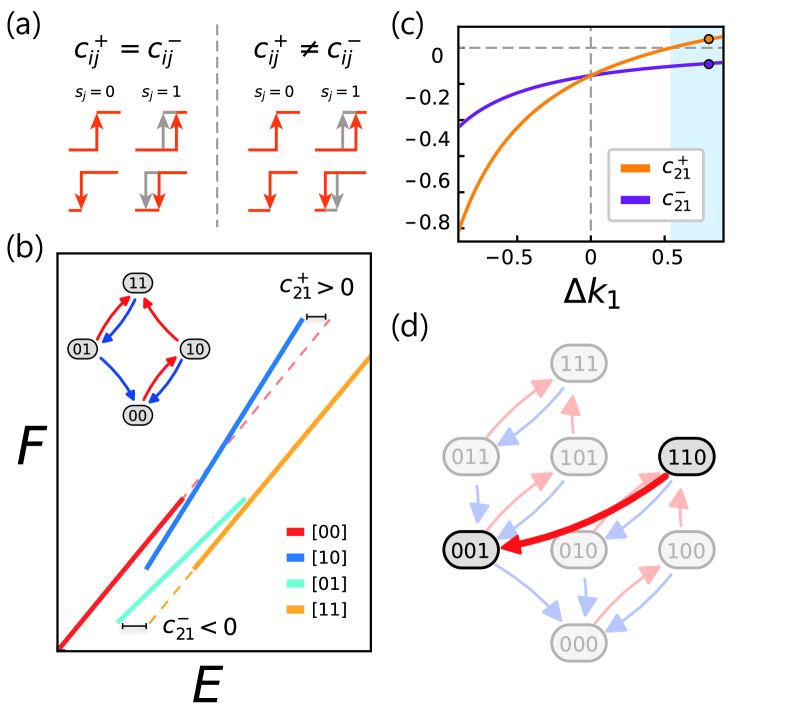
Without interactions, hysteron switches up when is increased above the bare switching field , and down when is decreased below . Interactions are encoded by introducing state dependent switching fields111Note that each state of hysterons requires (not ) critical fields , so that the switching thresholds of one hysteron depend on the phases of the others [21, 17]. For pairwise interactions the number of free parameters reduces to , yielding the ’canonical form’ [23, 4, 13]:
| (1) |
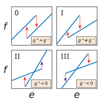
where are interaction coefficients. Assuming ’up-down’ symmetry (), reduces to (Fig. 2a); assuming reciprocity () further reduces to [18, 24]. Finally, in the absence of interactions (the so-called Preisach model) and [15, 22]. While the power of hysteron models is that they condense an energy landscape onto a set of switching fields, their Achilles heel is their lack of specific models for the switching fields and interaction coefficients.
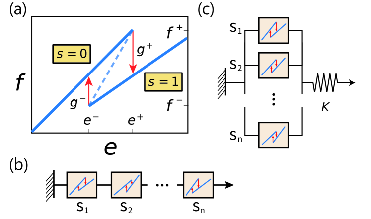
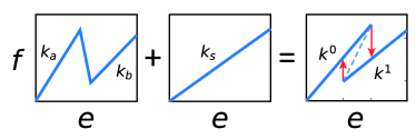
To explicitly calculate the switching fields for a given physical system, we now consider networks of physical hysterons. Each hysteron is characterized by a bilinear hysteretic relation between two conjugate physical variables, such as current and voltage [35], pressure and volume or flow [28, 36, 37], or, as we use here, force and displacement [29, 13] (Fig. 1):
| (2) |
where () is the stiffness at (), and is the intersection of the branch with the axis. These parameters determine the force jumps at the instabilities (Fig. 1a; see SI). is hysteretic between two local switching displacements . When physical hysterons are connected in a network, we can determine the switching fields and interactions as follows: (i) freeze the state so that the force-displacement relations are strictly linear; (ii) use force balance to determine as function of the driving ; (iii) determine state-dependent switching fields by calculating the values of where (Fig. 2b).
Linear networks.— We first consider mechanical hysterons in serial or parallel geometries (Fig. 1c-d). The corresponding force balance equations are scalar and, when the total displacement is controlled (), they produce pairwise interactions in the canonical form222Serially coupled hysterons do not experience interactions under controlled force [13]. For , parallel hysterons under controlled are non-interacting, and under controlled can be mapped to serially coupled hysterons under controlled .. These can be worked out explicitly from the collective force-displacement curves (Fig. 2b; see SI for the mapping to Eq. 1 and expressions for ). For serial coupling we obtain
| (3) |
For parallel coupling an additional spring of stiffness mediates the interactions (Fig. 1d) and we obtain:
| (4) |
For stiffness-symmetric hysterons (), the interactions are thus up-down symmetric () and global, i.e., hysteron affects all others equally (). Moreover, while serial coupling leads to [13], parallel coupling leads to : geometry controls the interactions. For stiffness-asymmetric hysterons (), the up-down symmetry is broken (as seen in experiments [4]) and tunable by , such that for large asymmetries and may even have opposite signs (Fig. 2c).
First, these interactions may produce avalanches whose up-down sequences follow from the signs of : (i) Symmetric hysterons in serial geometries produce avalanches that alternate between and and are of maximal length two [13]; (ii) Stiffness-asymmetric hysterons produce exotic, ’dissonant’ avalanches like , where an decrease in leads to an increase in the magnetization or vice versa333Crucially, the dissonant avalanches here are sequential. If the first hysteron triggers more than one flip, we consider the avalanche ill-defined due to race conditions [23] (Fig. 2d) [23]; (iii) In parallel geometries, both types of hysterons produce monotonic avalanches (only ’s or ’s) of arbitrary length. Recently, a new class of counter-snapping hysterons have been realized - where up (down) instabilities counter-intuitively lead to force jumps (drops) as opposed to the hysterons discussed here [38]. Our framework is directly generalizable to such cases by simply changing the sign of . This can lead to monotonic (alternating) avalanches in series (parallel), as we demonstrate in the SI.
Second, the t-graphs of linear networks all feature simple ’Preisach’ scaffolds, namely the switching order of the hysterons is state independent. This limits their complexity [39, 23, 13, 21]. It occurs because all hysterons experience the same force (displacement) in serial (parallel) networks, so that the scaffold follows the ordering of the critical forces (displacements ) [13].
Third, we numerically explored the range of t-graphs for three hysterons using random sampling [23, 13]. Their statistics appear in the SI. Out of hundreds of t-graphs, the vast majority obeys a hierarchical structure of nested loops leading to loop-return point memory (l-RPM), which hinders the emergence of complex behavior [39]; several t-graphs that break l-RPM lead to transients of length two under cyclic driving [17, 4, 13]. We also observe with low probability some longer avalanches, including a avalanche (for asymmetric hysterons in series). Hence, while we can control the (signs of) interactions by the hysteron parameters and geometry, the absence of scrambling in linear geometries severely limits their range of pathways and memory effects (see SI and [23, 4]).
2D networks.— Our understanding of the linear geometries suggests that 2D networks of hysterons may lead to scrambling, thus opening a route to advanced behavior such as multiperiodic responses where the system revisits its initial state after multiple driving cycles [18, 24]. We thus consider the paradigmatic case of a trigonal hub, where the two fixed and one moving corner of a triangle connect to a central, freely moving point via three symmetric hysterons with (Fig. 3a). Strikingly, the resulting interactions are controlled by the angles between hysterons and can become non-pairwise additive (i.e. more complex than the canonical form).
We derive exact expressions for the switching fields and interaction coefficients, using vectorial force balance on . For example, for , we obtain:
| (5) |
where () specify the geometry just before the transition for (), and .
This expression can be simplified in the limit , namely when the changes in length of the hysterons at instabilities are small so that the angles are essentially constant. In this limit, interactions are pairwise, up-down symmetric, and do not depend on the initial states. They can be simply expressed as:
| (6) |
where the geometrical factor arises from the connectivity of the trigonal hub (), is the mean angle between and at the instability of hysteron , averaged over . This expression has a clear geometrical interpretation. First, the jump between the branches, , provides the typical scale for the strength of interactions, as in the linear networks. Second, the factor represents how global driving is coupled to stretching of hysteron . Third, the factor captures the geometric coupling: consistent with our findings for serial and parallel couplings, this factor approaches -1 (1) for (), and approaches zero for perpendicular hysterons.
When , the angle changes are significant. Interactions are neither pairwise nor up-down symmetric, and depend on the initial states, e.g., (see SI). Yet, Eq. 6 still holds geometrical intuition, e.g., flipping may change . If as a result crosses , and have opposite signs (Fig. 3b; see Suppl. Video 1).
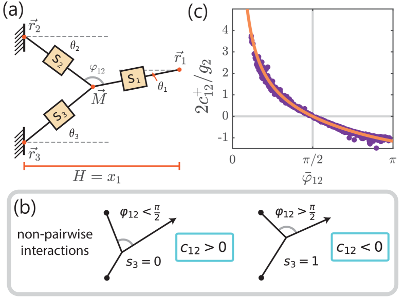
We complement our analytical analysis with numerical simulations, where we determine using overdamped dynamics: , where is a large damping constant and the forces are given by Eq. (2). Starting from any state we quasi-statically drive , follow and identify instabilities whenever . We find that the numerically calculated interaction coefficient closely matches the geometrical expression Eq. (6) (Fig. 3c; see SI for simulation parameters).
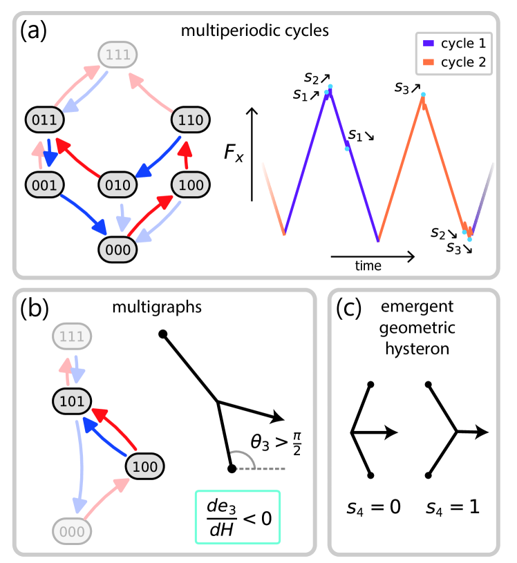
2D t-graphs.— The range of t-graphs that can be realized by 2D networks is huge, and we use our numerical scheme to generalize earlier t-graph sampling protocols [23, 13] to explore their diversity. First, we find that hysterons in a trigonal hub can easily host multiperiodic cycles (Fig. 4; see Suppl. Video 2). Such cycles are a hallmark of the complex behavior of interacting hysterons but cannot be realized in linear geometries as they require scrambling.
Second, the trigonal hub produces pathways where starting from a certain stable state , either increasing or decreasing the drive triggers the same transition. This violates the assumption of all hysteron models that transitions under increased (decreased) driving field are initiated by a hysteron flipping up (down). However, this effect can easily be understood geometrically, and is a general feature of higher dimensional networks: If the angle () between a hysteron and the driving is around , both an increase and a decrease of can lead to stretching of this hysteron, thus triggering the same flipping (Eq. 6). Such transitions lead to t-graph that is a multigraph (Fig. 4b; see Suppl, Video 3)444Multigraphs can occur in abstract hysteron models via avalanches [23], but here neither of the multitransitions are avalanches.. Similarly, both for and , the hysterons get stretched and all switch to phase 1 — hence, there is no guarantee that the hysterons reaches both phases for extreme driving.
Finally, networks can give rise to the emergence of buckling induced bistable degrees of freedom (Fig. 4c). This geometric degree of freedom can be mapped to an additional (fourth) hysteron, for example by defining its phase via left-or right leaning of the buckled structure [40]. Such geometric hysterons produce a wide variety of t-graphs, where we note that the saturated states (observed for extreme driving) generally include but not (see SI).
Conclusion and Outlook.— Networks of physical hysterons provide a direct link between real space configurations and interacting hysteron models. In particular, we have shown how geometry controls the sign and magnitude of the interactions which can become non-pair wise in the trigonal hub, and by extension, in larger 2D networks. Such network geometries also clarify that the unavoidable variation of the coupling between global driving and local deformations, potentially enhanced by non-affine deformations [41], can lead to non-monotonic behavior that exceeds current hysteron models. Together, our work demonstrates the potential for enhanced memory capabilities in hysteron networks [30].
We briefly mention directions for future research. First, straighforward extensions include 2D networks with stiffness asymmetry, self-crossing hysterons [38], general non-linearities, or mechanical hysterons with other degrees of freedom (e.g. shear or rotation) [31, 42, 43]. Second, the complex, non-pairwise interactions in 2D networks may provide a route to understanding the emergence of glassy dynamics in large networks [44, 45]. Third, our approach provides a route to avoid the occurrence of spurious loops, where after instability, the system cannot find a stable state but instead gets trapped in a infinite cycle. Such loops overwhelm hysteron models with arbitrary switching fields for large and/or strong interactions [23, 18, 21, 46], and also arise in coupled spin models [47]. While general conditions on the switching fields that avoid loops are missing [46], we note that physics-derived interactions do not lead to such loops; hence physical models allow to define ensembles of hysteron paramaters and interactions that lead to well-defined behavior. Finally, our explicit expressions for the geometry controlled interactions suggest that solving the inverse problem, i.e., translating a targeted pathway, t-graph, or set of switching fields to a specific hysteron network, is now within reach.
I Acknowledgements
We thank Yoav Lahini, Paul Baconnier, Lishuai Jin, Colin Meulblok, and Margot Teunisse for insightful discussions. We are also grateful to Muhittin Mungan and Yair Shokef for a careful reading of the manuscript. This work was funded by the European Research Council Grant ERC-101019474. D.S. acknowledges support from the Clore Israel Foundation.
II Supplemental Information
Appendix A 1. Bilinear Physical Hysterons
We consider mechanical hysterons where each of the two branches of the force-extension curve is linear. Their stiffness at is , and at is , so that tunes the stiffness asymmetry between the and branches. These hysterons are assumed to have zero rest length ( the branch crosses through ), the branch features an offset . These hysterons switch branch when the critical extensions are exceeded; specifically, when , ; similarly, , . These critical switching extensions define critical switching forces (the forces just before the instability): and . Finally, for (), the force jump ().
We can now classify hysterons based on their mechanical properties. We refer to symmetric hysterons with , or , as type 0. Asymmetric hysterons with , and both and , are referred to as type 1. Such hysterons with unequal natural stiffness can easily be realized [48]. Recently, bistable elements with self-crossing hysteresis loops have also been realized [38], yielding hysterons where either or . We refer to these respectively as type II and type III. We require that the overall dissipation is positive (). This classification is summarized in Fig. 5.
We note that hysterons based on two other conjugated variables can similarly be classified, connected and studied. These electronic elements with hysteretic voltage-current responses [35]; inflatable elements with hysteretic pressure-volume curves [37, 28]; or fluidic devices with hysteretic pressure-flow curves [36].
Physically, such hysterons are usually constructed by combining an element with a non-monotonic force-displacement curve, as shoiwn in Fig. 6. We consider a trilinear element, coupled to a spring of stiffness . Describing the trilinear element requires five parameters: The stiffness of the first branch ; the stiffness of the third branch ; the intersection of (the continuation of) the third branch with the axis ; the force at the first kink ; and the force at the second kink .
Coupled in series, the first branch reads
| (7) |
and the third branch
| (8) |
where we conveniently defined , , and .
We now consider the endpoints of these branches. This occurs when the force reaches . We denote these critical displacements and . The condition for an emergent hysteresis loop is simply that
| (9) |
Appendix B 2. Transition graphs, scaffolds, avalanches and scrambling
The t-graphs of coupled hysteron models feature nodes that represent the stable states and edges that represent the transitions from state to state that occur when is increased (decreased) past the relevant switching field. We can think of the t-graphs as composed of a scaffold that is dressed by (avalanche) transitions [21]. To define the scaffold, we first associate each state with a pair of critical hysterons and , which are the first hysterons that flip or when is increased or decreased:
| (10) |
where we note that the saturated states have only one critical hysteron. The scaffold is the collection of critical hysterons at all stable states [21]. Finally, we denote the landing states obtained by flipping the respective critical hysterons as and .
We now distinguish two types of transitions between states: single step transitions and avalanches. Denote the value of that initiates the transition as , then the stability of the landing states at determines the type of transition. For single step transitions, the landing state is stable at , and is one of the landing states; for avalanches, the landing state is unstable at , triggering additional transitions. However, note that all intermediate avalanches follow the scaffold. Hence. any possible transition is given by stitching together one or more steps specified by the scaffold [21].
We distinguish two classes of scaffolds: Preisach scaffolds and scrambled scaffolds [4, 23]: For Preisach scaffolds, the critical hysterons follow from a state-independent ordering of the upper and lower switching fields; hence if , then . All possible Preisach scaffolds can easily be generated from the Preisach model of non-interacting hysterons [22]. The much more numerous scrambled scaffolds feature state dependent orderings of their switching fields, so that the critical hysterons of different states are decoupled, allowing, e.g., and [23]. While t-graphs with avalanches based on a Preisach scaffold can exhibit non-trival properties, such as breaking of return point memory and transients [13], many more advanced properties are believed to require scrambling [23].
Appendix C 3. Mapping to abstract model for serially coupled hysterons
We consider mechanical hysterons coupled in series. We denote their state , where , representing the short and long configurations of the element respectively. We denote their individual forces and displacements and . Serial coupling boundary conditions dictates
| (11) |
| (12) |
We extend the existing framework of [13] by considering a varying stiffness for each hysteron. The stiffness at the () branch is (). is the stiffness difference that can take either positive or negative values. Conveniently, we write the force of the element as
| (13) |
where the stiffness difference is coupled to . is the intersection of the branch with the axis. The force drop is , while the force drop is . Next, force balance between elements gives
| (14) |
Plugging into Eq. 11 gives
| (15) |
Where we have denoted , the average inverse stiffness at ; and , the stiffness asymmetry. We have absorbed all state dependencies to the sum. This sum term, which represents the interactions with other elements , show that interactions do not exhibit ’up-down’ symmetry. To this end, we can map the system to the hysteron model
| (16) |
Where is the external field; are the bare thresholds; and , the interactions at and respectively (consistent with the notation for ).
We gauge out the self interaction (namely, we set ). This gauge is naturally consistent with the geometric interpretation for interactions presented in the main text. Altogether, the mapping gives
| (17) | |||||
| (18) | |||||
| (19) | |||||
| (20) | |||||
| (21) | |||||
| (22) |
The difference between the up and down interaction coefficients reads simply
| (23) |
Appendix D 4. Mapping to abstract model for parallelly coupled hysterons
We consider hysterons coupled in parallel, and allow their stiffnesses , to vary. If these are rigidly coupled so that , there are no interactions under controlled . However, when this assembly of hysterons is coupled in series to a Hookean spring of stiffness , length , and rest length , effective interactions arise. This geometry is described by:
| (24) | |||||
| (25) | |||||
| (26) |
| (27) |
Plugging this expression to Eq. 25, and using, we obtain:
| (28) |
As before, we use the expression for the state dependent switching fields to obtain the parameters of the abstract hysteron model:
| (29) | |||||
| (30) | |||||
| (31) | |||||
| (32) | |||||
| (33) | |||||
| (34) |
Hence, ferromagnetic interactions whose strength is inversely proportional to the spring constant emerge between parallely coupled hysterons. As for the serial case, including asymmetry () may introduce Anti-ferromagnetic interactions. Yet, similarly, these are by definition not capable of inducing AF avalanches. At each instability there’s a force drop and consequentially all elements can only increase their length.
The difference between the up and down interaction coefficients reads
| (35) |
Appendix E 5. Sampling t-graphs and avalanches
We now discuss the properties and statistics of t-graphs and avalanches, sampled for and for different hysteron types and different linear geometries. We draw random parameter sets for each type and each geometry (serial or parallel). Table 1 summarizes our results.
The first block summarizes the coupling coefficients for each type and geometry. For asymmetric hysterons, the possible signs of and are nearly freely controllable. For type II (type III) they are limited as by construction (), see Eqs. 23 and 35.
The second block shows the number of distinct t-graph topologies that we observed, and the number of these that obey l-RPM [39]. For type 0, it is possible to enumerate all possible t-graphs [13]. For the other, asymmetric hysterons, we did not manage to exhaustively sample the high-dimensional parameter space, even with parameter sets, so our numbers are lower bounds.
The third block summarizes the avalanche types. As discussed in the text, avalanches are inherited from the signs of interaction coefficients . We observe three types of avalanches. (i) Alternating (alt) avalanches, which go back and forth between and flips. The Preisach scaffold that underlies all t-graphs in linear geometries limits these to be of length 2 (namely or ) [13]. They are driven by negative, antiferromagnetic interactions, namely in series or in parallel; (ii) Dissonant (disso) avalanches, where increasing the driving leads to a decrease in the magnetization , or vice versa ( or ). These require a combination of negative and positive interactions, hence requiring asymmetry; (iii) Monotonic (mono) avalanches which only involve transitions or transitions. These are driven by positive, ferromagnetic interactions, namely in series or in parallel.
For example, type 0 hysterons in parallel have only positive interactions (), and therefore only exhibit monotonic avalanches. As another example, for type II hysterons in series, we have and . Therefore we find monotonic avalanches when increasing , and alternating avalanches when decreasing . Due to the asymmetry, dissonant avalanches can also occur when decreasing . All the table entries can be worked out by considering the signs of interactions and force jumps and following this logic.
We note that longer mixed avalanches (which combine and flips) also exist yet are extremely rare. We observed a single length 4 avalanche for type I hysterons in series (probability ). This avalanche occurs when a dissonant avalanche is extended with one extra flip. By symmetry, avalanches should exist yet were not sampled. Furthermore, even longer avalanches are expected to exist in larger systems.
| Coupling coefficients | Sampling statistics | Avalanches | |||||||
|---|---|---|---|---|---|---|---|---|---|
| Network | sym.? | signs of | # t-graphs | # l-RPM | type | ||||
| Serial 0 | Y | 44 | 37 | alt | . | . | |||
| Serial I | N | 100 | 77 | alt / disso | |||||
| Serial II | N | 66 | 57 | mono / alt | |||||
| Serial III | N | 66† | 57† | alt / mono | |||||
| Parallel 0 | Y | 58 | 58 | mono | |||||
| Parallel I | N | 137 | 116 | mono | |||||
| Parallel II | N | 52 | 45 | alt / mono | . ‡ | ||||
| Parallel III | N | 52† | 45† | mono / alt | . ‡ | ||||
Appendix F 6. Trigonal hub geometry
We consider three hysterons coupled in a 2D geometry as illustrated in Fig. 3a. For simplicity we set and . The hysterons are freely rotating and can change their angles which are defined with respect to the horizontal axis. The external ends are pinned at , while the central point is free to move on both axes. The horizontal displacement of the system is controlled externally. Without loss of generality, we set it as the external field . We also set . The boundary conditions now depend on . In the axis we have
| (36) |
where we denoted .
In the axis we denote
| (37) |
| (38) |
where and are constants given by the geometry. This represents the fact that distances in the axis are fixed (since we drive along ).
Force balance on the central point gives
| (39) |
| (40) |
F.1 6.1. - a representative example
We focus on the interaction exerts on the transition , and follow the full derivation.
| (41) |
Naively, one could suggest the following mapping to a hysteron model
| (42) | |||
| (43) | |||
| (44) | |||
| (45) |
However, this mapping turns to be incorrect. Its bare thresholds and interaction coefficients depend on the angles . These are in turn determined by force balance in a non-linear manner, and obtain different values for different states . As the angles are different in each state we expect . Furthermore, activating hysteron will change all angles and therefore the coupling . Namely, interactions are no longer pairwise. To understand the geometry dependence of interactions, let us focus on the interaction that exerts on as a representative example.
The interaction coefficient includes changes in the bare threshold induced by flipping . We denote the angles and the angles at which reaches instability , at and respectively. The interaction coefficient reads
| (46) |
We shall show that, in fact, represents an intuitive and repeatable geometric dependence in the limit . It is already apparent that in this limit . Thus for convenience we mark the smaller terms in teal.
To simplify the calculation we treat the three terms , , separately.
For the first term we have
| (47) |
where we used . We denote the average angle.
To resolve , we now examine . This is simply the vertical displacement of the central point, between the two instabilities. It’s exact value can be obtained from force balance in the axis. At the instability we have
| (50) | |||
| (51) |
Subtracting the two equations we get
| (52) |
Now, we explicitly subtract the sines on the LHS using to get
| (53) |
| (54) |
We can now write the second term of Eq. 61 as
| (55) |
Combining all contributions we get
| (56) | ||||
or if we subtract the sines explicitly
| (57) | ||||
We can now use the approximation , namely that flipping hysterons induces small length changes. In other words, this means that each instability also leads to small changes in the rest angles. Therefore, we can approximate , or . This allows to simplify the above expression. First, we can drop the term. Second, we can replace with , the angle formed between and . This gives
| (58) |
In this form, Eq. 58 can be understood through a simple geometrical intuition. First, the strength of the interaction is proportional to . This angle determines how switching changes the length . Next, the threshold diverges as . This represents how external driving stretches . Finally, matches the analytical 1d solution when and ( is serially coupled to which are coupled in parallel).
We can even simplify further: for mechanical balance give a simple relation . It turns to hold for large angles on average, and we can approximate by an equation with one parameter only:
| (59) |
Thus, geometry dependence of interactions is systematic despite the breakdown of the simple mapping to the hysteron model.
This derivation also shows explicitly that interactions are inherently non-pairwise, and sheds light on their nature. When displacements at instabilities are large, namely , the coefficient explicitly depends on . Furthermore, flipping has another indirect effect - by varying the angle . This provides intuition for the emergence of strong non-pairwise interactions. If flipping changes such that it crosses when is flipped, the interaction can change its sign. In essence, changing the geometry can toggle between positive and negative (parallel-like and serial-like) coupling.
F.2 6.2. All coefficients
We can now derive all interaction coefficients in a similar manner. We begin with the up coefficients
Due to relabeling symmetry between and , it suffices to consider and .
Similarly to Eq. 41, we write as a function of :
| (60) |
The first coefficient reads
| (61) |
where we have used the same notation of angles, this time with respect to the instability and both states of . Neglecting the smaller term from gives our previous derivation, with relabeling between and and multiplying by 2:
| (62) |
The next coefficient reads
| (63) |
This expression is yet again similar to Eq. 61, but the second term has a plus sign instead of a minus sign, because and are at the opposite side of , compared to the central point . Explicitly subtracting the cosines in the first term (as done above), now gives a minus sign for the same reason
| (64) |
Altogether this gives
| (65) |
having plugged .
This concludes the derivation for the up coefficients . For the down coefficients we have exactly the same derivation, with the addition of a negligible term from . For example, reads
| (66) |
The last term will give a minute correction, which is negligible when we approximate . Thus Eq. 58 holds here as well. Note that in this limit, the angles at both and instabilities are the same, therefore .
Altogether we have a unified formula for all coefficients:
| (67) |
with being a geometrical factor that arises from the connectivity of the trigonal hub, , , and the angles assessed with respect to the instability . As noted above, the interaction coefficients are top-down symmetric, i.e. .
Appendix G 7. Emergent geometric hysteron in 2D
Aside of its three built-in hysterons, the trigonal hub geometry can host additional bistable degrees of freedom which arise from geometric non-linearities [40]. When is manipulated externally, the edges of hysterons , can buckle to the left or to the right of the axis so that two stable states with the central point and may emerge (see Fig. 4). The transitions between these states are hysteretic [40]. Such buckling occurs if the rest lengths of two hysterons and are together longer than the distance between them (). So far, we have considered type 0 hysterons with rest length at () equal to (); in the remainder of this section, we consider a positive rest-length for , by taking the force displacement relation .
We now associate the global buckling mode to an additional hysteron, denoting () for states with (). We include this hysteron in the numerical scheme for t-graph sampling, and identify changes in by tracking . We randomize the hysteron parameters , , , and , and compute the corresponding t-graphs systematically. Indeed, exhibits hysteretic transitions. Note that we do not limit self-intersection, namely the edges of the hub are free to cross each other without an additional steric interaction.
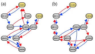
The range of transition graphs proliferates with the emergent degree of freedom . Fig. 7 shows several examples. We stress, however, that an exhaustive sampling of the parameter space and graph properties is difficult, and a task we leave to future works. Instead, we highlight a peculiar feature that signals the breakdown of naive hysteron models. In the trigonal hub, saturated states (where all hysterons are at the 0 or 1 state) are not necessarily absorbing states which define a closed loop in the transition graph [39]. Instead, the absorbing states (highlighted in Fig. 7) are and , namely when all three hysterons are in the long state, and the whole trigonal hub is polarized to the left () or to the right ().
Appendix H 8. Figure parameters
In this section we provide the hysteron parameters corresponding to the figures of the main text and supplementary videos.
Fig. 2b,c - Two hysterons of type I are coupled in series. The corresponding parameters are: ; ; ; ; ; ; . For panel c we calculate for different values of asymmetry , while the rest of the parameters are fixed.
Fig. 2d - Three hysterons of type I are coupled in series, and exhibit a dissonant avalanche. The corresponding parameters are: ; ; ; ; ; ; . Note that here we allow . As explained in previous sections, the hysteresis is emergent from the coupling of several elements, such that the hysteron model satisfies .
Fig. 3b - Three hysterons of type 0 are connected in a trigonal hub. We randomize sets of positions and parameters. Importantly, we draw and , thus maintaining the approximation used to derive the interaction coefficient .
Fig. 4a - Three hysterons of type 0 are connected in a trigonal hub, and exhibit a multiperiodic cycle of period , when driven along . The corresponding parameters are: ; ; ; ; ; .
Fig. 4b - Three hysterons of type 0 are connected in a trigonal hub, and give rise to a multigraph, where from state driving either up or down leads to the same transition . The corresponding parameters are: ; ; ; ; ; .
Appendix I 9. Supplementary videos
This section accompanies the supplementary movies, in which we visualize some exotic behaviors and pathways exhibited by the trigonal hub. The notation is as follows: hysterons are labeled in the same order as in the main text ( on the right, on the top left, and on the bottom left); short hysterons are colored in blue; long hysterons are colored in red.
Suppl. video 1 - Three hysterons of type 0 are connected in a trigonal hub, and demonstrate strong non-pairwise interactions, where flipping changes the sign of . In the video, we examine the instability for both states of . When , hysteron promotes hysteron to flip earlier, therefore . When , hysteron hinders hysteron from flipping, therefore and the interaction has changed its sign. Note that visually, in the former case , while in the latter case as discussed in the main text.
The corresponding parameters here are: ; ; ; ; .
Suppl. video 2 - This video visualizes the multiperiodic cycle of Figure 4a in the main text. starting from , after one full cycle the hub arrives at . It returns back to the initial state only after a second driving cycle, thus realizing a multiperiodic cycle with a period . The hysteron parameters appear in the previous section.
Suppl. video 3 - This video visualizes the multigraph shown in Figure 4b in the main text. Here, starting from and , driving either up or down leads to the same transition . Notice that is rather perpendicular to the driving axis. When is decreased so that is stretched, in other words due to the geometry of the hub. The hysteron parameters appear in the previous section.
References
- Mungan et al. [2019] M. Mungan, S. Sastry, K. Dahmen, and I. Regev, Networks and hierarchies: How amorphous materials learn to remember, Physical review letters 123, 178002 (2019).
- Regev et al. [2021] I. Regev, I. Attia, K. Dahmen, S. Sastry, and M. Mungan, Topology of the energy landscape of sheared amorphous solids and the irreversibility transition, Physical Review E 103, 062614 (2021).
- Keim et al. [2020] N. C. Keim, J. Hass, B. Kroger, and D. Wieker, Global memory from local hysteresis in an amorphous solid, Physical Review Research 2, 012004 (2020).
- Bense and van Hecke [2021] H. Bense and M. van Hecke, Complex pathways and memory in compressed corrugated sheets, Proceedings of the National Academy of Sciences 118, e2111436118 (2021).
- Shohat et al. [2022] D. Shohat, D. Hexner, and Y. Lahini, Memory from coupled instabilities in unfolded crumpled sheets, Proceedings of the National Academy of Sciences 119, e2200028119 (2022).
- Keim et al. [2019] N. C. Keim, J. D. Paulsen, Z. Zeravcic, S. Sastry, and S. R. Nagel, Memory formation in matter, Reviews of Modern Physics 91, 035002 (2019).
- Galloway et al. [2022] K. Galloway, E. Teich, X. Ma, C. Kammer, I. Graham, N. Keim, C. Reina, D. Jerolmack, A. Yodh, and P. Arratia, Relationships between structure, memory and flow in sheared disordered materials, Nature Physics 18, 565 (2022).
- Keim and Nagel [2011] N. C. Keim and S. R. Nagel, Generic transient memory formation in disordered systems with noise, Physical review letters 107, 010603 (2011).
- Paulsen et al. [2014] J. D. Paulsen, N. C. Keim, and S. R. Nagel, Multiple transient memories in experiments on sheared non-brownian suspensions, Physical review letters 113, 068301 (2014).
- Mukherji et al. [2019] S. Mukherji, N. Kandula, A. Sood, and R. Ganapathy, Strength of mechanical memories is maximal at the yield point of a soft glass, Physical review letters 122, 158001 (2019).
- Shohat and Lahini [2023] D. Shohat and Y. Lahini, Dissipation indicates memory formation in driven disordered systems, Physical Review Letters 130, 048202 (2023).
- Kwakernaak and van Hecke [2023] L. J. Kwakernaak and M. van Hecke, Counting and sequential information processing in mechanical metamaterials, Physical Review Letters 130, 268204 (2023).
- Liu et al. [2024] J. Liu, M. Teunisse, G. Korovin, I. R. Vermaire, L. Jin, H. Bense, and M. van Hecke, Controlled pathways and sequential information processing in serially coupled mechanical hysterons, Proceedings of the National Academy of Sciences 121, e2308414121 (2024).
- Treml et al. [2018] B. Treml, A. Gillman, P. Buskohl, and R. Vaia, Origami mechanologic, Proceedings of the National Academy of Sciences 115, 6916 (2018).
- Preisach [1935] F. Preisach, Über die magnetische nachwirkung, Zeitschrift für physik 94, 277 (1935).
- Paulsen and Keim [2019] J. D. Paulsen and N. C. Keim, Minimal descriptions of cyclic memories, Proceedings of the Royal Society A 475, 20180874 (2019).
- Lindeman and Nagel [2021] C. W. Lindeman and S. R. Nagel, Multiple memory formation in glassy landscapes, Science Advances 7, eabg7133 (2021).
- Keim and Paulsen [2021] N. C. Keim and J. D. Paulsen, Multiperiodic orbits from interacting soft spots in cyclically sheared amorphous solids, Science Advances 7, eabg7685 (2021).
- Jules et al. [2022] T. Jules, A. Reid, K. E. Daniels, M. Mungan, and F. Lechenault, Delicate memory structure of origami switches, Physical Review Research 4, 013128 (2022).
- Ding and van Hecke [2022] J. Ding and M. van Hecke, Sequential snapping and pathways in a mechanical metamaterial, The Journal of Chemical Physics 156 (2022).
- Teunisse and van Hecke [2024] M. H. Teunisse and M. van Hecke, Transition graphs of interacting hysterons: Structure, design, organization and statistics, arXiv preprint arXiv:2404.11344 (2024).
- Terzi and Mungan [2020] M. M. Terzi and M. Mungan, State transition graph of the preisach model and the role of return-point memory, Physical Review E 102, 012122 (2020).
- van Hecke [2021] M. van Hecke, Profusion of transition pathways for interacting hysterons, Physical Review E 104, 054608 (2021).
- Szulc et al. [2022] A. Szulc, M. Mungan, and I. Regev, Cooperative effects driving the multi-periodic dynamics of cyclically sheared amorphous solids, The Journal of Chemical Physics 156 (2022).
- Jalowiec et al. [2023] T. R. Jalowiec, C. W. Lindeman, and N. C. Keim, Isolating the enhanced memory of a glassy system, arXiv preprint arXiv:2306.07177 (2023).
- Kumar et al. [2022] D. Kumar, S. Patinet, C. E. Maloney, I. Regev, D. Vandembroucq, and M. Mungan, Mapping out the glassy landscape of a mesoscopic elastoplastic model, The Journal of Chemical Physics 157 (2022).
- Nicolas et al. [2018] A. Nicolas, E. E. Ferrero, K. Martens, and J.-L. Barrat, Deformation and flow of amorphous solids: Insights from elastoplastic models, Reviews of Modern Physics 90, 045006 (2018).
- Muhaxheri and Santangelo [2024] G. Muhaxheri and C. D. Santangelo, Bifurcations of inflating balloons and interacting hysterons, arXiv preprint arXiv:2403.10721 (2024).
- Puglisi and Truskinovsky [2000] G. Puglisi and L. Truskinovsky, Mechanics of a discrete chain with bi-stable elements, Journal of the Mechanics and Physics of Solids 48, 1 (2000).
- Sirote-Katz et al. [2024] C. Sirote-Katz, D. Shohat, C. Merrigan, Y. Lahini, C. Nisoli, and Y. Shokef, Emergent disorder and mechanical memory in periodic metamaterials, Nature Communications 15, 4008 (2024).
- Hyatt and Harne [2023] L. P. Hyatt and R. L. Harne, Programming metastable transition sequences in digital mechanical materials, Extreme Mechanics Letters 59, 101975 (2023).
- El Elmi and Pasini [2024] A. El Elmi and D. Pasini, Tunable sequential pathways through spatial partitioning and frustration tuning in soft metamaterials, Soft Matter 20, 1186 (2024).
- Yang et al. [2023] T. Yang, D. Hathcock, Y. Chen, P. L. McEuen, J. P. Sethna, I. Cohen, and I. Griniasty, Bifurcation instructed design of multistate machines, Proceedings of the National Academy of Sciences 120, e2300081120 (2023).
- Paulsen and Keim [2024] J. D. Paulsen and N. C. Keim, Mechanical memories in solids, from disorder to design, arXiv preprint arXiv:2405.08158 (2024).
- Strukov et al. [2008] D. B. Strukov, G. S. Snider, D. R. Stewart, and R. S. Williams, The missing memristor found, nature 453, 80 (2008).
- Martínez-Calvo et al. [2024] A. Martínez-Calvo, M. D. Biviano, A. H. Christensen, E. Katifori, K. H. Jensen, and M. Ruiz-García, The fluidic memristor as a collective phenomenon in elastohydrodynamic networks, Nature Communications 15, 3121 (2024).
- Djellouli et al. [2024] A. Djellouli, B. Van Raemdonck, Y. Wang, Y. Yang, A. Caillaud, D. Weitz, S. Rubinstein, B. Gorissen, and K. Bertoldi, Shell buckling for programmable metafluids, Nature 628, 545 (2024).
- Ducarme et al. [2024] P. Ducarme, B. Weber, M. van Hecke, and J. Overvelde, in preparation, (2024).
- Mungan and Terzi [2019] M. Mungan and M. M. Terzi, The structure of state transition graphs in systems with return point memory: I. general theory, in Annales Henri Poincaré, Vol. 20 (Springer, 2019) pp. 2819–2872.
- Lindeman et al. [2023] C. W. Lindeman, V. F. Hagh, C. I. Ip, and S. R. Nagel, Competition between energy and dynamics in memory formation, Physical review letters 130, 197201 (2023).
- Ellenbroek et al. [2009] W. G. Ellenbroek, Z. Zeravcic, W. van Saarloos, and M. van Hecke, Non-affine response: Jammed packings vs. spring networks, Europhysics Letters 87, 34004 (2009).
- Kamp et al. [2024] L. M. Kamp, M. Zanaty, A. Zareei, B. Gorissen, R. J. Wood, and K. Bertoldi, Reprogrammable sequencing for physically intelligent under-actuated robots, arXiv preprint arXiv:2409.03737 (2024).
- Paulsen [2024] J. D. Paulsen, Mechanical hysterons with tunable interactions of general sign, preprint (2024).
- Shohat et al. [2023] D. Shohat, Y. Friedman, and Y. Lahini, Logarithmic aging via instability cascades in disordered systems, Nature Physics 19, 1890 (2023).
- Shohat et al. [2024] D. Shohat, Y. Lahini, and D. Hexner, Are crumpled sheets marginally stable?, arXiv preprint arXiv:2408.08030 (2024).
- Baconnier and van Hecke [2024] P. Baconnier and M. van Hecke, in preparation, (2024).
- Eissfeller and Opper [1994] H. Eissfeller and M. Opper, Mean-field monte carlo approach to the sherrington-kirkpatrick model with asymmetric couplings, Physical Review E 50, 709 (1994).
- Meeussen and van Hecke [2023] A. Meeussen and M. van Hecke, Multistable sheets with rewritable patterns for switchable shape-morphing, Nature 621, 516 (2023).