Quaternion Nuclear Norm minus Frobenius Norm Minimization for Color Image Reconstruction

Abstract

Color image restoration methods typically represent images as vectors in Euclidean space or combinations of three monochrome channels. However, they often overlook the correlation between these channels, leading to color distortion and artifacts in the reconstructed image. To address this, we present Quaternion Nuclear Norm Minus Frobenius Norm Minimization (QNMF), a novel approach for color image reconstruction. QNMF utilizes quaternion algebra to capture the relationships among RGB channels comprehensively. By employing a regularization technique that involves nuclear norm minus Frobenius norm, QNMF approximates the underlying low-rank structure of quaternion-encoded color images. Theoretical proofs are provided to ensure the method’s mathematical integrity. Demonstrating versatility and efficacy, the QNMF regularizer excels in various color low-level vision tasks, including denoising, deblurring, inpainting, and random impulse noise removal, achieving state-of-the-art results.

1 Introduction

Color images find applications in various fields including video processing, computer vision, medical imaging, remote sensing, and multimedia processing. However, during generation, transmission, and storage, images unavoidably degrade due to factors like noise, blurring, downsampling, and other forms of corruption. This degradation can be represented by the equation:

$$\mathbf{Y}=\mathbf{A}\mathbf{X}+\mathbf{N},$$ (1)

where $\mathbf{X}$ represents the original image, $\mathbf{Y}$ represents the observed degraded image, $\mathbf{A}$ stands for a linear degradation operator, such as a blurring kernel, and $\mathbf{N}$ denotes additive independent Gaussian white noise with a zero mean. Eq. (1) poses a classical inverse problem due to its ill-posed nature, presenting significant challenges in data science, particularly in the realm of color image restoration methods.

Various research efforts have focused on solving image reconstruction problems using methods such as total variation (TV) [1], non-local self-similarity (NSS) [2, 3], dictionary learning [4, 5], low rank [6, 7], tensor [8, 9], and deep learning [10, 11]. While these algorithms have shown significant success with grayscale images, their application to color images has posed significant challenges. Grayscale images have a single channel, while color images have three channels: R, G, and B, exhibiting color correlation. Applying grayscale algorithms independently to each channel disrupts this correlation, leading to color artifacts and distortions in the final restored result.

Two successful strategies have been proposed to address the challenge of channel correlation in color images. The first strategy involves converting color images from the standard RGB space to a less correlated color space, such as YCbCr or HSV, and then independently denoising each channel of the converted image. Pioneering work in this approach extended block matching and 3D filtering (BM3D) [2] to color block matching and 3D filtering (CBM3D) [3]. CBM3D converts an sRGB image to a luminance-chrominance space, performs block matching in the luminance space, and then filters each channel independently. This approach has been followed by a substantial body of work [12]. In addition to the YCbCr space, other researchers have explored the opponent transformation [12]. Recently, Jia et al. [1] proposed the saturation-value total variation (SV-TV) for the HSV color space. These studies effectively circumvent the challenges posed by channel correlation through color space conversion. However, this conversion leads to a complex noise structure and can even result in the loss of noise independence, transforming it into correlated noise [13]. Furthermore, the conversion of color space does not effectively exploit the correlation between colors.

An alternative solution considers coupling between channels. This can be achieved by vectorizing the three channels, fully accounting for cross-channel information. Kong et al. [14] have further extended this approach by transforming color image patches into vectors, treating them as a unified entity. These methods allow for simultaneous processing of all three channels, unlike independent processing. They can also be generalized to a tensor form [8, 15], interpreting the color image as a multidimensional tensor with dimensions corresponding to the spatial and spectral channels. Xu et al. [16] noted that noise intensity is not always uniform across the three channels of a color image. To address this, they proposed a diagonal form of the weight matrix to model noise differences between the channels, an idea that was subsequently expanded upon [17]. However, this strategy reverts to independent channel processing when the noise intensity approaches uniformity, thereby losing the capacity for information exchange between channels.

Additionally, data-driven methods have demonstrated exceptional performance in image reconstruction. Deep learning, unlike traditional methods, primarily focuses on learning the mapping between degraded images and their corresponding clean images using pairwise data. Consequently, these methods circumvent the challenge of extending traditional algorithms from grayscale to color images. In 2016, Zhang et al. proposed DnCNN [10], a creative approach based on residual learning that significantly enhanced reconstruction performance. Since then, advancements in the deep learning community [18] have consistently surpassed state-of-the-art results for image reconstruction. Currently, the most advanced image reconstruction algorithms are based on Transformer [19] and diffusion models [20]. Despite the excellent performance of these deep learning algorithms, their computational complexity and high computational cost pose challenges for real-world applications.

The main challenge in color image restoration is effectively utilizing inter-channel correlation to minimize color distortion and artifacts while preserving image structure. Given the human visual system’s sensitivity to color, degradation from color anomalies significantly impacts subjective evaluations of image quality. Recent advances have been made in traditional algorithms for processing color images. Quaternions, generalizations of complex numbers, consist of a real part and three imaginary parts, precisely encoding the three channels of a color image. This captures the coupling relations between channels, allowing the color image to be processed as a whole, leveraging non-trivial algebraic structure. Quaternion multiplication facilitates complete information exchange between channels. Recent studies [21, 22] demonstrate that the color image processing method based on quaternion representation delivers excellent color image performance. Figure 1 succinctly illustrates the advantages of the quaternion method in color processing. In the smoothing region, even subtle processing errors between channels can lead to significant color artifacts, whereas the quaternion-based QNMF yields excellent visual results.

GT	SV-TV	CBM3D	McWNNM	QNMF

Figure 1: Comparison of color image denoising algorithms with different strategies in terms of color distortion and artifacts. The images are $45\times 45$ patches, sourced from the Kodak dataset, and are corrupted by noise with $\sigma=60$.

To better address color distortion and artifacts while preserving more image details, we propose a new nonconvex quaternion hybrid norm, termed the Quaternion Nuclear Norm Minus Frobenius Norm (QNMF). The QNMF effectively handles various rank components, enabling improved approximation of the rank norm. We employ QNMF as a quaternionic low-rank regularizer for a wide range of low-level vision tasks, thus enhancing algorithm performance and robustness. Additionally, we offer a rigorous mathematical proof to ensure the theoretical soundness of QNMF. The main contributions of this paper are as follows:

• To enhance the approximation of the rank norm, this paper introduces QNMF as a quaternionic low-rank regularizer, applicable to various color image tasks.

• We prove the global optimality of our proposed QNMF model and demonstrate the convergence of the algorithm.

• Numerous experiments were conducted, demonstrating that the proposed QNMF is capable of addressing various tasks including color image denoising, deblurring, matrix completion, and robust principal component analysis (RPCA), and achieved state-of-the-art results.

The paper is structured as follows: Section 2 covers the fundamentals of quaternion algebra and quaternion low-rank correlation methods. Our proposed nuclear norm minus Frobenius norm and its application to color image processing are introduced in Section 3. Section 4 presents simulation experiments comparing our approach with other state-of-the-art methods. Conclusions are outlined in Section 5.

2 Related work

2.1 Quaternion Basics

As a generalization of the real space $\mathbb{R}$ and the complex space $\mathbb{C}$, the quaternion space $\mathbb{Q}$ is defined as $\mathbb{Q}=\{a_{0}+a_{1}\mathbf{i}+a_{2}\mathbf{j}+a_{3}\mathbf{k}|a_{0},a_{1},a_{2},a_{3}\in\mathbb{R}\}$, where $\{1,\mathbf{i},\mathbf{j},\mathbf{k}\}$ forms a basis of $\mathbb{Q}$, and the imaginary units $\mathbf{i},\mathbf{j},\mathbf{k}$ satisfy $\mathbf{i}^{2}=\mathbf{j}^{2}=\mathbf{k}^{2}=\mathbf{i}\mathbf{j}\mathbf{k}=-1$, $\mathbf{i}\mathbf{j}=\mathbf{k}=-\mathbf{j}\mathbf{i}$, $\mathbf{j}\mathbf{k}=\mathbf{i}=-\mathbf{k}\mathbf{j}$, $\mathbf{k}\mathbf{i}=\mathbf{j}=-\mathbf{i}\mathbf{k}$. Quaternion multiplication, one of the most important properties of the quaternion space $\mathbb{Q}$, does not satisfy the law of exchange. For example, a quaternion variable is denoted by having a dot on the variable, such as $\dot{\mathbf{a}}$ and $\dot{\mathbf{A}}$.

Let $\dot{\mathbf{a}}=a_{0}+a_{1}\mathbf{i}+a_{2}\mathbf{j}+a_{3}\mathbf{k}\in\mathbb{Q}$, $\dot{\mathbf{b}}=b_{0}+b_{1}\mathbf{i}+b_{2}\mathbf{j}+b_{3}\mathbf{k}\in\mathbb{Q}$ and $\lambda\in\mathbb{R}$, their operations are

$$\dot{\mathbf{a}}+\dot{\mathbf{b}}=(a_{0}+b_{0})+(a_{1}+b_{1})\mathbf{i}+(a_{2}+b_{2})\mathbf{j}+(a_{3}+b_{3})\mathbf{k},$$

$$\lambda\dot{\mathbf{a}}=(\lambda a_{0})+(\lambda a_{1})\mathbf{i}+(\lambda a_{2})\mathbf{j}+(\lambda a_{3})\mathbf{k},$$

$$\dot{\mathbf{a}}\dot{\mathbf{b}}=(a_{0}b_{0}-a_{1}b_{1}-a_{2}b_{2}-a_{3}b_{3})+(a_{0}b_{1}+a_{1}b_{0}+a_{2}b_{3}-a_{3}b_{2})\mathbf{i}$$

$$~{}~{}+(a_{0}b_{2}-a_{1}b_{3}+a_{2}b_{0}+a_{3}b_{1})\mathbf{j}+(a_{0}b_{3}+a_{1}b_{2}-a_{2}b_{1}-a_{3}b_{0})\mathbf{k}.$$

The conjugate and modulus of $\dot{\mathbf{a}}$ are defined as

$$\dot{\mathbf{a}}^{*} =a_{0}-a_{1}\mathbf{i}-a_{2}\mathbf{j}-a_{3}\mathbf{k},$$ (2)

$$|\dot{\mathbf{a}}| =\sqrt{a_{0}^{2}+a_{1}^{2}+a_{2}^{2}+a_{3}^{2}}.$$

If $a_{0}=0$, $\dot{\mathbf{a}}$ is called pure quaternion. Each quaternion $\dot{\mathbf{a}}$ can be uniquely represented as

$$\dot{\mathbf{a}}=a_{0}+a_{1}\mathbf{i}+(a_{2}+a_{3}\mathbf{i})\mathbf{j}=c_{1}+c_{2}\mathbf{j},$$

where $c_{1}=a_{0}+a_{1}\mathbf{i}$ and $c_{2}=a_{2}+a_{3}\mathbf{i}$ are complex numbers.

For a quaternion matrix, defined as $\dot{\mathbf{X}}=(\dot{x}_{ij})\in\mathbb{Q}^{m\times n}$, where $\dot{\mathbf{X}}=\mathbf{X}_{0}+\mathbf{X}_{1}\mathbf{i}+\mathbf{X}_{2}\mathbf{j}+\mathbf{X}_{3}\mathbf{k}$ and $\mathbf{X}_{l}\in\mathbb{R}^{m\times n}(l=0,1,2,3)$ are real matrices. For a color image, it can be represented as a pure quaternion matrix with real part 0, i.e., each channel is represented as an imaginary part

$$\dot{\mathbf{X}}_{RGB}=\mathbf{X}_{R}\mathbf{i}+\mathbf{X}_{G}\mathbf{j}+\mathbf{X}_{B}\mathbf{k},$$ (3)

where $\mathbf{X}_{R}$, $\mathbf{X}_{G}$ and $\mathbf{X}_{B}$ are the R, G, and B channels of the color image.

The norms of quaternion vectors and matrices are defined as follows. The $l_{1}$ and $l_{2}$ norms of the quaternion vector are $||\dot{\mathbf{a}}||_{1}:=\sum_{i=0}^{3}|a_{i}|$ and $||\dot{\mathbf{a}}||_{2}:=\sqrt{\sum_{i=0}^{3}|a_{i}|^{2}}$, respectively. The Frobenius norm of a quaternionic matrix is $||\dot{\mathbf{X}}||_{F}:=\sqrt{\sum_{i,j}|\dot{x}_{ij}|^{2}}=\sqrt{\sum_{k}^{\min{\{i,j\}}}\sigma_{\dot{\mathbf{X}},k}^{2}}$, where $\sigma_{\dot{\mathbf{X}},k}$ denotes the $k$-th singular value. The singular value decomposition of a quaternion matrix $\dot{\mathbf{X}}$ is given by the following lemma.

Lemma 2.1.

(QSVD [23]) Given a quaternion matrix $\dot{\mathbf{X}}\in\mathbb{Q}^{m\times n}$ with rank $r$. There are two unitary quaternion matrices $\dot{\mathbf{U}}\in\mathbb{Q}^{m\times m}$ and $\dot{\mathbf{V}}\in\mathbb{Q}^{n\times n}$ satisfying $\dot{\mathbf{X}}=\dot{\mathbf{U}}\left(\begin{array}[]{cc}\mathbf{\Sigma_{r}}&0\\ 0&0\end{array}\right)\dot{\mathbf{V}}^{\top}$, where $\mathbf{\Sigma_{r}}=\mathrm{diag}(\sigma_{1},\dots,\sigma_{r})\in\mathbb{R}^{r\times r}$, and all singular values $\sigma_{i}>0,i=1,\dots,r$.

2.2 Quaternion Low Rank Methods

Real-valued low-rank methods excel in grayscale image processing but face hurdles with color images, often resulting in color distortion and artifacts due to disregarding RGB channel correlation. Recognizing the significance of inter-channel correlation, quaternion-based color image processing methods have garnered increasing interest in recent years.

Yu et al. [22] introduced quaternion-weighted nuclear norm minimization (QWNNM) for color image denoising, drawing inspiration from [6, 24]. Extending this approach, Huang et al. [25] adapted QWNNM for processing color image deblurring. Mathematically, QWNNM is defined as:

$$\min_{\dot{\mathbf{X}}}\frac{\gamma}{2}||\dot{\mathbf{A}}\dot{\mathbf{X}}-\dot{\mathbf{Y}}||^{2}_{F}+||\dot{\mathbf{X}}||_{w,*}$$ (4)

where $\dot{\mathbf{A}}\in\mathbb{Q}^{m\times m}$ represents a 2D quaternion degradation matrix, while $\dot{\mathbf{X}}$ and $\dot{\mathbf{Y}}$ stand for the potential image and the observed degraded image, respectively. The term $||\cdot||_{w,*}$ is defined as

$$||\dot{\mathbf{X}}||_{w,*}=\sum_{i}|w_{i}\sigma_{\dot{\mathbf{X}},i}|,$$

where $\sigma_{\dot{\mathbf{X}},i}$ is the $i$-th singular value of $\dot{\mathbf{X}}$ and the weight $w_{i}$ is computed as $w_{i}=\frac{c}{\sigma_{\dot{\mathbf{X}},i}+\epsilon}$, where $c$ is a constant and $\epsilon$ is a small number.

The studies by Yu et al. [22] and Huang et al. [25] illustrate the effectiveness of quaternion representation in color image processing by leveraging inter-channel correlation. Combining the weighted Schatten p-norm minimization [26] with quaternion representation, Zhang et al. [27] proposed the QWSNM model, defined as:

$$||\dot{\mathbf{X}}||_{w,S_{p}}=\left(\sum_{i=1}^{\min{\{n,m\}}}w_{i}\sigma_{\dot{\mathbf{X}},i}^{p}\right)^{\frac{1}{p}},$$ (5)

where $p>0$. The QWSNM offers precise control over each singular value. Notably, when $p=1$, QWNNM emerges as a special instance of QWSNM. However, the inclusion of the Schatten p-norm increases the computational complexity of QWSNM relative to QWNNM.

Several recent works [28, 29] have highlighted that convex alternatives to rank norms can yield suboptimal solutions. In response, various nonconvex alternatives to rank norms have emerged [21, 30]. Building upon these insights, we introduce a novel quaternion nonconvex hybrid norm, termed quaternion nuclear norm minus Frobenius norm, tailored for color image processing.

3 Quaternion Nuclear Norm minus Frobenius Norm Minimization

In this section, we introduce the quaternion nuclear norm minus Frobenius norm minimization (QNMF) problem, extending it to the image linear inverse problem.

3.1 QNMF model

To address the color image denoising problem, we propose a novel approach by combining quaternion representation with the nuclear-Frobenius hybrid norm. This leads to the formulation of the quaternion nuclear norm minus Frobenius norm minimization problem:

$$\dot{\mathbf{X}}=\arg\min_{\dot{\mathbf{X}}}\frac{1}{2}||\dot{\mathbf{Y}}-\dot{\mathbf{X}}||^{2}_{F}+\lambda(||\dot{\mathbf{X}}||_{*}-\alpha||\dot{\mathbf{X}}||_{F}),$$ (6)

where $\dot{\mathbf{Y}}$ represents the observed noisy color image, and $\lambda>0$ and $\alpha>0$ are regularization parameters. The global optimal solution of model (6) can be obtained according to the following theorem.

Theorem 3.1.

Given $\dot{\mathbf{Y}}\in\mathbb{Q}^{m\times n}$, without loss of generality, we assume that $m\geq n$. Let $\dot{\mathbf{Y}}=\dot{\mathbf{U}}\mathbf{\Sigma_{\dot{Y}}}\dot{\mathbf{V}}^{\top}$ be the QSVD of $\dot{\mathbf{Y}}$, where $\mathbf{\Sigma_{\dot{Y}}}=\mathrm{diag}(\sigma_{\dot{\mathbf{Y}},1},\sigma_{\dot{\mathbf{Y}},2},\dots,\sigma_{\dot{\mathbf{Y}},m})$. The global optimum of model (6) can be expressed as $\dot{\mathbf{X}}=\hat{\dot{\mathbf{U}}}\mathbf{\Sigma_{\dot{X}}}\hat{\dot{\mathbf{V}}}^{\top}$, where $\mathbf{\Sigma_{\dot{X}}}=\mathrm{diag}(\sigma_{\dot{\mathbf{X}},1},\sigma_{\dot{\mathbf{X}},2},\dots,\sigma_{\dot{\mathbf{X}},m})$ is a diagonal nonnegative matrix and $(\sigma_{\dot{\mathbf{X}},1},\sigma_{\dot{\mathbf{X}},2},\dots,\sigma_{\dot{\mathbf{X}},m})$ is the solution to the following optimization problem:

$$\arg \min_{\mathbf{\Sigma_{\dot{X}}}}\frac{1}{2}||\mathbf{\Sigma_{\dot{Y}}}-\mathbf{\Sigma_{\dot{X}}}||^{2}_{2}+\lambda(||\mathbf{\Sigma_{\dot{X}}}||_{1}-\alpha||\mathbf{\Sigma_{\dot{X}}}||_{2})$$ (7)

$$\mathrm{s.t.}\sigma_{\dot{\mathbf{X}},1}\geq\sigma_{\dot{\mathbf{X}},2}\geq\dots\geq\sigma_{\dot{\mathbf{X}},m}\geq 0,$$

and the globally optimal solution $\mathbf{\tilde{\Sigma}_{\dot{X}}}$ is $\mathbf{\tilde{\Sigma}_{\dot{X}}}=\frac{||\mathbf{z}||_{2}+\alpha\lambda}{||\mathbf{z}||_{2}}\mathbf{z}$, where $\mathbf{z}=\max(\mathbf{\Sigma_{\dot{Y}}}-\lambda,0)$.

Proof.

Let $\dot{\mathbf{X}}=\hat{\dot{\mathbf{U}}}\mathbf{\Sigma_{\dot{X}}}\hat{\dot{\mathbf{V}}}^{\top}$ and $\dot{\mathbf{Y}}=\dot{\mathbf{U}}\mathbf{\Sigma_{\dot{Y}}}\dot{\mathbf{V}}^{\top}$ be the QSVD decomposition of $\dot{\mathbf{X}}$ and $\dot{\mathbf{Y}}$.

$$\frac{1}{2}||\dot{\mathbf{Y}}-\dot{\mathbf{X}}||^{2}_{F}+\lambda(||\dot{\mathbf{X}}||_{*}-\alpha||\dot{\mathbf{X}}||_{F})$$ (8)

$$=\frac{1}{2}\mathrm{tr}(\dot{\mathbf{Y}}^{\top}\dot{\mathbf{Y}}+\dot{\mathbf{X}}^{\top}\dot{\mathbf{X}}-2\dot{\mathbf{X}}^{\top}\dot{\mathbf{Y}})+\lambda(||\dot{\mathbf{X}}||_{*}-\alpha||\dot{\mathbf{X}}||_{F})$$

$$=\frac{1}{2}(||\mathbf{\Sigma_{\dot{Y}}}||^{2}_{2}+||\mathbf{\Sigma_{\dot{X}}}||^{2}_{2})-\mathrm{tr}(\dot{\mathbf{X}}^{\top}\dot{\mathbf{Y}})+\lambda||\mathbf{\Sigma_{\dot{X}}}||_{1}-\lambda\alpha||\mathbf{\Sigma_{\dot{X}}}||_{2}.$$

According to the Von Neumann’s trace inequality, when $\dot{\mathbf{U}}=\hat{\dot{\mathbf{U}}}$ and $\dot{\mathbf{V}}=\hat{\dot{\mathbf{V}}}$, $\mathrm{tr}(\dot{\mathbf{X}}^{\top}\dot{\mathbf{Y}})\leq\mathbf{\Sigma_{\dot{X}}}^{\top}\mathbf{\Sigma_{\dot{Y}}}$. Then solving (6) can be instead computed by solving $\mathbf{\Sigma_{\dot{X}}}$ as

$$\arg \min_{\mathbf{\Sigma_{\dot{X}}}}\frac{1}{2}||\mathbf{\Sigma_{\dot{Y}}}-\mathbf{\Sigma_{\dot{X}}}||^{2}_{2}+\lambda(||\mathbf{\Sigma_{\dot{X}}}||_{1}-\alpha||\mathbf{\Sigma_{\dot{X}}}||_{2})$$ (9)

$$\mathrm{s.t.}\sigma_{\dot{\mathbf{X}},1}\geq\sigma_{\dot{\mathbf{X}},2}\geq\dots\geq\sigma_{\dot{\mathbf{X}},m}\geq 0,$$

where $\mathbf{\Sigma_{\dot{X}}}=\mathrm{diag}(\sigma_{\dot{\mathbf{X}},1},\sigma_{\dot{\mathbf{X}},2},\dots,\sigma_{\dot{\mathbf{X}},m})$. According to [31], the global optimal solution of model (9) can be obtained by

$$\mathbf{\tilde{\Sigma}_{\dot{X}}}=\frac{||\mathbf{z}||_{2}+\alpha\lambda}{||\mathbf{z}||_{2}}\mathbf{z},$$ (10)

where $\mathbf{z}=\max(\mathbf{\Sigma_{\dot{Y}}}-\lambda,0)$. ∎

According to Theorem 3.1, the globally optimal solution for the model (6) can be expressed as $\tilde{\dot{\mathbf{X}}}=\dot{\mathbf{U}}\mathbf{\tilde{\Sigma}_{\dot{X}}}\dot{\mathbf{V}}^{\top}$. Larger singular values hold more information and should be shrunk less. Therefore, we adjust the shrinkage threshold $\lambda$ accordingly. If $\sigma_{\dot{\mathbf{Y}},i}\leq\lambda$, we keep the current shrinkage threshold: $z_{i}=\max(\sigma_{\dot{\mathbf{Y}},i}-\lambda,0)=0$. However, if $\sigma_{\dot{\mathbf{Y}},i}>\lambda$, we reduce the shrinkage threshold to $\lambda/2$: $z_{i}=\sigma_{\dot{\mathbf{Y}},i}-\lambda/2$. We observe that $\frac{||\mathbf{z}||_{2}+\alpha\lambda/2}{||\mathbf{z}||_{2}}>1$, which could lead to $\tilde{\sigma}_{\dot{\mathbf{X}},i}=\frac{||\mathbf{z}||_{2}+\alpha\lambda/2}{||\mathbf{z}||_{2}}z_{i}>\sigma_{\dot{\mathbf{Y}},i}$. This is not allowed in singular value shrinkage. To prevent this, when $\frac{||\mathbf{z}||_{2}+\alpha\lambda/2}{||\mathbf{z}||_{2}}z_{i}>\sigma_{\dot{\mathbf{Y}},i}$, we set $\tilde{\sigma}_{\dot{\mathbf{X}},i}=\sigma_{\dot{\mathbf{Y}},i}$. In conclusion, the final solution for $\mathbf{\tilde{\Sigma}_{\dot{X}}}$ is presented as follows:

$$\tilde{\sigma}_{\dot{\mathbf{X}},i}=\left\{\begin{array}[]{cl}\sigma_{\dot{\mathbf{Y}},i},&\mathrm{if}\enspace\sigma_{\dot{\mathbf{Y}},i}>\frac{K\lambda}{2(K-1)};\\ K(\sigma_{\dot{\mathbf{Y}},i}-\lambda/2),&\mathrm{if}\enspace\lambda<\sigma_{\dot{\mathbf{Y}},i}\leq\frac{K\lambda}{2(K-1)};\\ 0,&\mathrm{if}\enspace\sigma_{\dot{\mathbf{Y}},i}\leq\lambda.\\ \end{array}\right.$$ (11)

where $K=1+\frac{\alpha\lambda}{2||\mathbf{z}||_{2}}$, $\mathbf{z}=\mathrm{diag}(z_{1},z_{2},\dots,z_{m})$, and

$$z_{i}=\left\{\begin{array}[]{cl}\sigma_{\dot{\mathbf{Y}},i}-\lambda/2,&\mathrm{if}\enspace\sigma_{\dot{\mathbf{Y}},i}>\lambda;\\ 0,&\mathrm{if}\enspace\sigma_{\dot{\mathbf{Y}},i}\leq\lambda.\end{array}\right.$$

Figure 2(a) illustrates the shrinkage process described in Eq. (11) on a $35\times 35$ patch with $\sigma=60$. We compare our proposed QNMF method with previous studies such as QWNNM [22] and QWSNM [27]. Similar to QWNNM and QWSNM, QNMF applies less shrinkage to larger singular values, but it avoids complex weight calculations. A key distinction is that QNMF offers a closed-form solution, eliminating the need for iterative shrinkage and simplifying computations. Figure 2(b) shows the variation in shrinkage among the three methods. QNMF incorporates truncation to prevent excessive increases in singular values, setting $\tilde{\sigma}_{\dot{\mathbf{X}},i}=\sigma_{\dot{\mathbf{Y}},i}$ when $\sigma_{\dot{\mathbf{Y}},i}>\frac{K\lambda}{2(K-1)}$. This approach is similar to truncated nuclear norms (TNN) [32], but with a significant difference: while TNN uses a fixed truncation threshold, QNMF adjusts dynamically.

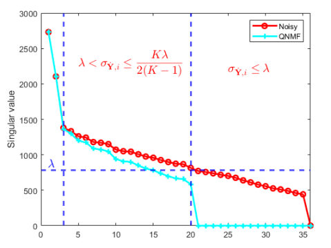
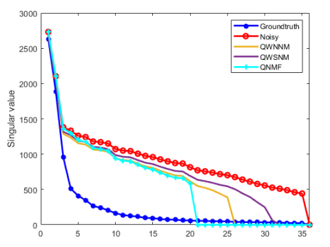
(a)	(b)

Figure 2: Singular value shrinkage diagrammed.

3.2 QNMF for image linear inverse problem

We extend QNMF to the image linear inverse problem given by:

$$\dot{\mathbf{X}}=\arg\min_{\dot{\mathbf{X}}}\frac{\gamma}{2}||\dot{\mathbf{A}}\dot{\mathbf{X}}-\dot{\mathbf{Y}}||^{2}_{F}+\lambda(||\dot{\mathbf{X}}||_{*}-\alpha||\dot{\mathbf{X}}||_{F})$$ (12)

where $\dot{\mathbf{A}}\in\mathbb{Q}^{m\times m}$ represents a 2D quaternion degradation matrix.For instance, if $\dot{\mathbf{A}}=\dot{\mathbf{I}}$, it pertains to the denoising problem discussed in subsection 3.1. Alternatively, if $\dot{\mathbf{A}}$ denotes a blur kernel, it corresponds to color image deblurring. $\dot{\mathbf{X}}\in\mathbb{Q}^{m\times n}$ and $\dot{\mathbf{Y}}\in\mathbb{Q}^{m\times n}$ represent the original and degraded images, respectively.

We utilize the alternating direction multiplier method (ADMM) to solve the model (12). This involves introducing an auxiliary variable $\dot{\mathbf{Z}}$ with the constraint $\dot{\mathbf{X}}=\dot{\mathbf{Z}}$, and the Lagrange multiplier $\dot{\mathbf{\eta}}$. The augmented Lagrange function of (12) is then expressed as

$$\mathcal{L}(\dot{\mathbf{X}},\dot{\mathbf{Z}},\dot{\mathbf{\eta}},\beta) =\frac{\gamma}{2}||\dot{\mathbf{A}}\dot{\mathbf{X}}-\dot{\mathbf{Y}}||^{2}_{F}+\lambda(||\dot{\mathbf{Z}}||_{*}-\alpha||\dot{\mathbf{Z}}||_{F})+\frac{\beta}{2}||\dot{\mathbf{X}}-\dot{\mathbf{Z}}||_{F}^{2}+\langle{\dot{\bm{\eta}},\dot{\mathbf{X}}-\dot{\mathbf{Z}}}\rangle.$$ (13)

where $\beta>0$ is the penalty parameter. The update strategy for (13) is as follows:

$$\left\{\begin{aligned} \dot{\mathbf{X}}^{(k+1)}&=\arg\min_{\dot{\mathbf{X}}}\mathcal{L}(\dot{\mathbf{X}},\dot{\mathbf{Z}}^{(k)},\dot{\mathbf{\eta}}^{(k)},\beta^{(k)}),\\ \dot{\mathbf{Z}}^{(k+1)}&=\arg\min_{\dot{\mathbf{Z}}}\mathcal{L}(\dot{\mathbf{X}}^{(k+1)},\dot{\mathbf{Z}},\dot{\mathbf{\eta}}^{(k)},\beta^{(k)}),\\ \dot{\mathbf{\eta}}^{(k+1)}&=\dot{\mathbf{\eta}}^{(k)}+\beta^{(k)}(\dot{\mathbf{X}}^{(k+1)}-\dot{\mathbf{Z}}^{(k+1)}),\\ \beta^{(k+1)}&=\mu\beta^{(k)},\quad(\mu>1).\\ \end{aligned}\right.$$ (14)

The minimization (13) readily splits into two subproblems: $\dot{\mathbf{X}}$ and $\dot{\mathbf{Z}}$.

The $\dot{\mathbf{X}}$ sub-problem is written as

$$\dot{\mathbf{X}}=\arg\min_{\dot{\mathbf{X}}}\frac{\gamma}{2}||\dot{\mathbf{A}}\dot{\mathbf{X}}-\dot{\mathbf{Y}}||^{2}_{F}+\frac{\beta}{2}||\dot{\mathbf{X}}-\dot{\mathbf{Z}}||_{F}^{2}+\langle{\dot{\mathbf{\eta}},\dot{\mathbf{X}}-\dot{\mathbf{Z}}}\rangle.$$ (15)

By quaternion theory [33], the closed solution of the problem is

$$\dot{\mathbf{X}}=(\gamma\dot{\mathbf{A}}^{*}\dot{\mathbf{A}}+\beta\dot{\mathbf{I}})^{-1}(\gamma\dot{\mathbf{A}}^{*}\dot{\mathbf{Y}}+\beta\dot{\mathbf{Z}}-\dot{\mathbf{\eta}}).$$ (16)

The left inverse of a quaternion matrix is defined as follows: if a quaternion matrix $\dot{\mathbf{U}}$ is known and there exists a quaternion matrix $\dot{\mathbf{V}}$ such that $\dot{\mathbf{V}}\dot{\mathbf{U}}=\mathbf{I}$, then $\dot{\mathbf{V}}$ is the left inverse of $\dot{\mathbf{U}}$, denoted as $\dot{\mathbf{U}}^{-1}$. To avoid complex inverse operations, this can be efficiently solved using the quaternion fast Fourier transform [34].

According to (13), the $\dot{\mathbf{Z}}$ subproblem can be reformulated as

$$\dot{\mathbf{Z}}=\arg\min_{\dot{\mathbf{Z}}}\,\lambda(||\dot{\mathbf{Z}}||_{*}-\alpha||\dot{\mathbf{Z}}||_{F})+\frac{\beta}{2}||\dot{\mathbf{Z}}-(\dot{\mathbf{X}}+\frac{\dot{\mathbf{\eta}}}{\beta})||_{F}^{2}.$$ (17)

Therefore, the $\dot{\mathbf{Z}}$ subproblem can be solved using (11). The entire optimization process is summarized in Algorithm 1. Subsequently, we provide weak convergence results for Algorithm 1.

Theorem 3.2.

Suppose that the parameter sequence $\{\beta^{(k)}\}$ is unbounded and the sequences $\{\dot{\mathbf{X}}^{(k)}\}$ and $\{\dot{\mathbf{Z}}^{(k)}\}$ are generated by Algorithm 1, which satisfies:

$$\lim_{k\rightarrow+\infty}||\dot{\mathbf{X}}^{(k+1)}-\dot{\mathbf{Z}}^{(k+1)}||_{F}=0,$$ (18)

$$\lim_{k\rightarrow+\infty}||\dot{\mathbf{X}}^{(k+1)}-\dot{\mathbf{X}}^{(k)}||_{F}=0,$$ (19)

$$\lim_{k\rightarrow+\infty}||\dot{\mathbf{Z}}^{(k+1)}-\dot{\mathbf{Z}}^{(k)}||_{F}=0.$$ (20)

The detailed proof of Theorem 3.2 is available in Appendix A. It’s noteworthy that the proof hinges on the unboundedness of $\beta^{(k)}$. Rapid increases in $\beta^{(k)}$ can prematurely halt iterations, hindering the attainment of a satisfactory solution. Thus, smaller $\mu$ values are employed in the experiments to restrain the rapid growth of $\beta^{(k)}$.

1

Input :  Observation $\dot{\mathbf{Y}}$; Initialize $\dot{\mathbf{X}}^{(0)}=\dot{\mathbf{Y}}$, $\dot{\mathbf{Z}}^{(0)}=\dot{\mathbf{X}}^{(0)}$, $\dot{\mathbf{\eta}}^{(0)}=0$; Parameters $\gamma$, $\lambda$, $\beta$, $\mu$, $\alpha$, $K$;

2

Output :  The reconstructed image $\dot{\mathbf{X}}^{(K)}$;

3

4for $k=0,1,\dots,K-1$ do

5      Update $\dot{\mathbf{X}}^{(k+1)}$ by (16) ;

6      Update $\dot{\mathbf{Z}}^{(k+1)}$ by (17) ;

7      Update $\dot{\mathbf{\eta}}^{(k+1)}=\dot{\mathbf{\eta}}^{(k)}+\beta^{(k)}(\dot{\mathbf{X}}^{(k+1)}-\dot{\mathbf{Z}}^{(k+1)})$ ;

8      Update $\beta^{(k+1)}=\mu\beta^{(k)}$ ;

9     

10      end for

Algorithm 1 QNMF Algorithm

3.3 QNMF for matrix completion

In this section, we apply QNMF to tackle the matrix completion problem and introduce a model based on QNMF:

$$\min_{\dot{\mathbf{X}}}||\dot{\mathbf{X}}||_{*}-\alpha||\dot{\mathbf{X}}||_{F}\quad s.t\quad\mathcal{P}_{\Omega}(\dot{\mathbf{X}})=\mathcal{P}_{\Omega}(\dot{\mathbf{Y}}),$$ (21)

where $\Omega$ is a binary mask matrix of the same size as $\dot{\mathbf{Y}}$. Zeroes in $\Omega$ indicate unobserved values. $\mathcal{P}_{\Omega}(\dot{\mathbf{Y}})=\Omega\odot\dot{\mathbf{Y}}$, where $\odot$ denotes the Hadamard product. This constraint ensures consistency between the estimated $\dot{\mathbf{X}}$ and the observed $\dot{\mathbf{Y}}$ at the observed entries.

By introducing the auxiliary variable $\dot{\mathbf{Z}}$, and the Lagrange multiplier $\dot{\mathbf{\eta}}$, the augmented Lagrange function for (21) is expressed as:

$$\mathcal{L}(\dot{\mathbf{X}},\dot{\mathbf{Z}},\dot{\mathbf{\eta}},\beta) =\lambda(||\dot{\mathbf{X}}||_{*}-\alpha||\dot{\mathbf{X}}||_{F})+\frac{\beta}{2}||\dot{\mathbf{Y}}-\dot{\mathbf{X}}-\dot{\mathbf{Z}}||_{F}^{2}$$ (22)

$$~{}~{}~{}+\langle{\dot{\mathbf{\eta}},\dot{\mathbf{Y}}-\dot{\mathbf{X}}-\dot{\mathbf{Z}}}\rangle\quad s.t\quad\mathcal{P}_{\Omega}(\dot{\mathbf{Z}})=0.$$

The update strategy for (22) is as follows:

$$\left\{\begin{aligned} \dot{\mathbf{Z}}^{(k+1)}&=\arg\min_{\dot{\mathbf{Z}}}\mathcal{L}(\dot{\mathbf{X}}^{(k+1)},\dot{\mathbf{Z}},\dot{\mathbf{\eta}}^{(k)},\beta^{(k)}),\quad s.t\quad||\mathcal{P}_{\Omega}(\dot{\mathbf{Z}})||_{F}^{2}=0,\\ \dot{\mathbf{X}}^{(k+1)}&=\arg\min_{\dot{\mathbf{X}}}\mathcal{L}(\dot{\mathbf{X}},\dot{\mathbf{Z}}^{(k)},\dot{\mathbf{\eta}}^{(k)},\beta^{(k)}),\\ \dot{\mathbf{\eta}}^{(k+1)}&=\dot{\mathbf{\eta}}^{(k)}+\beta^{(k)}(\dot{\mathbf{Y}}-\dot{\mathbf{X}}^{(k+1)}-\dot{\mathbf{Z}}^{(k+1)}),\\ \beta^{(k+1)}&=\mu\beta^{(k)},\quad(\mu>1).\\ \end{aligned}\right.$$ (23)

The $\dot{\mathbf{Z}}$ subproblem is

$$\dot{\mathbf{Z}}=\arg\min_{\dot{\mathbf{Z}}}\,||\dot{\mathbf{Y}}-\dot{\mathbf{Z}}+\frac{\dot{\mathbf{\eta}}}{\beta}-\dot{\mathbf{X}}||_{F}^{2}\;s.t\;||\mathcal{P}_{\Omega}(\dot{\mathbf{Z}})||_{F}^{2}=0.$$ (24)

This quadratic problem can be easily solved. The $\dot{\mathbf{X}}$ subproblem is

$$\dot{\mathbf{X}}=\arg\min_{\dot{\mathbf{X}}}\,\lambda(||\dot{\mathbf{X}}||_{*}-\alpha||\dot{\mathbf{X}}||_{F})+\frac{\beta}{2}||(\dot{\mathbf{Y}}-\dot{\mathbf{Z}}+\frac{\dot{\mathbf{\eta}}}{\beta})-\dot{\mathbf{X}}||_{F}^{2}.$$ (25)

The solution of this subproblem is therefore given in (11). The entire algorithmic procedure is described in Algorithm 2.

Theorem 3.3.

Suppose that the parameter sequence $\{\beta^{(k)}\}$ is unbounded and the sequences $\{\dot{\mathbf{X}}^{(k)}\}$ and $\{\dot{\mathbf{Z}}^{(k)}\}$ are generated by Algorithm 2, which satisfies:

$$\lim_{k\rightarrow+\infty}||\dot{\mathbf{X}}^{(k+1)}-\dot{\mathbf{X}}^{(k)}||_{F}=0,$$ (26)

$$\lim_{k\rightarrow+\infty}||\dot{\mathbf{Y}}-\dot{\mathbf{X}}^{(k+1)}-\dot{\mathbf{Z}}^{(k+1)}||_{F}=0.$$ (27)

The proof of Theorem 3.3 mirrors that of Theorem 3.4 discussed subsequently; refer to the proof of Theorem 3.4 for specifics. It is not reiterated in this paper.

1

Input :  Observation $\dot{\mathbf{Y}}$; Mask matrix $\Omega$; Initialize $\dot{\mathbf{X}}^{(0)}=\dot{\mathbf{Y}}$, $\dot{\mathbf{\eta}}^{(0)}=0$; Parameters $\lambda$, $\beta$, $\mu$, $\alpha$, $K$;

2

Output :  The reconstructed image $\dot{\mathbf{X}}^{(K)}$;

3

4for $k=0,1,\dots,K-1$ do

5      Update $\dot{\mathbf{Z}}^{(k+1)}$ by (24) ;

6      Update $\dot{\mathbf{X}}^{(k+1)}$ by (25) ;

7      Update $\dot{\mathbf{\eta}}^{(k+1)}=\dot{\mathbf{\eta}}^{(k)}+\beta^{(k)}(\dot{\mathbf{Y}}-\dot{\mathbf{X}}^{(k+1)}-\dot{\mathbf{Z}}^{(k+1)})$ ;

8      Update $\beta^{(k+1)}=\mu\beta^{(k)}$ ;

9     

10      end for

Algorithm 2 QNMF-MC Algorithm

3.4 QNMF for robust PCA

In practice, observed data are often corrupted by outliers or sparse noise, significantly impacting the Frobenius norm data fidelity term used in low-rank estimation. To address this issue, Candés et al. [35] introduced robust principal component analysis (RPCA) based on the nuclear norm, utilizing the $\mathcal{L}1$-norm for modeling errors. Building upon this, we extend QNMF to RPCA, resulting in a QNMF-based RPCA model:

$$\min_{\dot{\mathbf{X}},\dot{\mathbf{Z}}}\lambda(||\dot{\mathbf{X}}||_{*}-\alpha||\dot{\mathbf{X}}||_{F})+\rho||\dot{\mathbf{Z}}||_{1}\;s.t\;\dot{\mathbf{Y}}=\dot{\mathbf{X}}+\dot{\mathbf{Z}}.$$ (28)

where $\dot{\mathbf{Z}}$ is sparse error. According to ADMM, its augmented Lagrange function is

$$\mathcal{L}(\dot{\mathbf{X}},\dot{\mathbf{Z}},\dot{\mathbf{\eta}},\beta) =\lambda(||\dot{\mathbf{X}}||_{*}-\alpha||\dot{\mathbf{X}}||_{F})+\rho||\dot{\mathbf{Z}}||_{1}+\frac{\beta}{2}||\dot{\mathbf{Y}}-\dot{\mathbf{X}}-\dot{\mathbf{Z}}||_{F}^{2}+\langle{\dot{\mathbf{\eta}},\dot{\mathbf{Y}}-\dot{\mathbf{X}}-\dot{\mathbf{Z}}}\rangle.$$ (29)

The update strategy for (29) is as follows:

$$\left\{\begin{aligned} \dot{\mathbf{Z}}^{(k+1)}&=\arg\min_{\dot{\mathbf{Z}}}\mathcal{L}(\dot{\mathbf{X}}^{(k+1)},\dot{\mathbf{Z}},\dot{\mathbf{\eta}}^{(k)},\beta^{(k)}),\\ \dot{\mathbf{X}}^{(k+1)}&=\arg\min_{\dot{\mathbf{X}}}\mathcal{L}(\dot{\mathbf{X}},\dot{\mathbf{Z}}^{(k)},\dot{\mathbf{\eta}}^{(k)},\beta^{(k)}),\\ \dot{\mathbf{\eta}}^{(k+1)}&=\dot{\mathbf{\eta}}^{(k)}+\beta^{(k)}(\dot{\mathbf{Y}}-\dot{\mathbf{X}}^{(k+1)}-\dot{\mathbf{Z}}^{(k+1)}),\\ \beta^{(k+1)}&=\mu\beta^{(k)},\quad(\mu>1).\\ \end{aligned}\right.$$ (30)

The $\dot{\mathbf{Z}}$ subproblem is

$$\dot{\mathbf{Z}}=\arg\min_{\dot{\mathbf{Z}}}\,\rho||\dot{\mathbf{Z}}||_{1}+\frac{\beta}{2}||(\dot{\mathbf{Y}}-\dot{\mathbf{X}}+\frac{\dot{\mathbf{\eta}}}{\beta})-\dot{\mathbf{Z}}||_{F}^{2}.$$ (31)

According to the soft-threshold shrinkage, the solution for $\dot{\mathbf{Z}}$ is

$$\dot{\mathbf{Z}}=\frac{\dot{\mathbf{Y}}-\dot{\mathbf{X}}+\frac{\dot{\mathbf{\eta}}}{\beta}}{\left|\dot{\mathbf{Y}}-\dot{\mathbf{X}}+\frac{\dot{\mathbf{\eta}}}{\beta}\right|+\epsilon}\max\left(\left|\dot{\mathbf{Y}}-\dot{\mathbf{X}}+\frac{\dot{\mathbf{\eta}}}{\beta}\right|-\frac{\rho}{\beta},0\right),$$ (32)

where $|\cdot|$ is the modulus of the quaternion and $\epsilon$ is a small number. The $\dot{\mathbf{X}}$ subproblem is consistent with (25). The whole algorithmic procedure is described in Algorithm 3.

1

Input :  Observation $\dot{\mathbf{Y}}$; Initialize $\dot{\mathbf{X}}^{(0)}=\dot{\mathbf{Y}}$, $\dot{\mathbf{Z}}^{(0)}=0$, $\dot{\mathbf{\eta}}^{(0)}=0$; Parameters $\rho$, $\lambda$, $\beta$, $\mu$, $\alpha$, $K$;

2

Output :  The reconstructed image $\dot{\mathbf{X}}^{(K)}$;

3

4for $k=0,1,\dots,K-1$ do

5      Update $\dot{\mathbf{Z}}^{(k+1)}$ by (32) ;

6      Update $\dot{\mathbf{X}}^{(k+1)}$ by (25) ;

7      Update $\dot{\mathbf{\eta}}^{(k+1)}=\dot{\mathbf{\eta}}^{(k)}+\beta^{(k)}(\dot{\mathbf{Y}}-\dot{\mathbf{X}}^{(k+1)}-\dot{\mathbf{Z}}^{(k+1)})$ ;

8      Update $\beta^{(k+1)}=\mu\beta^{(k)}$ ;

9     

10      end for

Algorithm 3 QNMF-RPCA Algorithm

Theorem 3.4.

Suppose that the parameter sequence $\{\beta^{(k)}\}$ is unbounded and the sequences $\{\dot{\mathbf{X}}^{(k)}\}$ and $\{\dot{\mathbf{Z}}^{(k)}\}$ are generated by Algorithm 3, which satisfies:

$$\lim_{k\rightarrow+\infty}||\dot{\mathbf{X}}^{(k+1)}-\dot{\mathbf{X}}^{(k)}||_{F}=0,$$ (33)

$$\lim_{k\rightarrow+\infty}||\dot{\mathbf{Z}}^{(k+1)}-\dot{\mathbf{Z}}^{(k)}||_{F}=0.$$ (34)

$$\lim_{k\rightarrow+\infty}||\dot{\mathbf{Y}}-\dot{\mathbf{X}}^{(k+1)}-\dot{\mathbf{Z}}^{(k+1)}||_{F}=0.$$ (35)

The proof details of Theorem 3.4 are provided in the supplementary material.

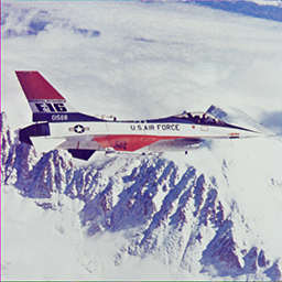
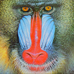
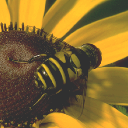
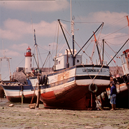
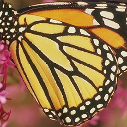
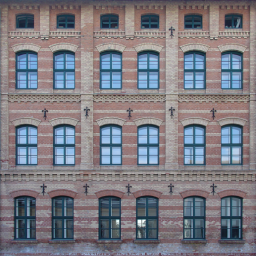
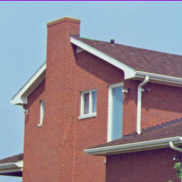
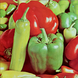
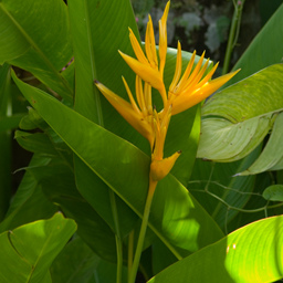
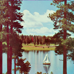
Figure 3: CSet12.

4 Experiments

4.1 Experiment Setting

In this section, we conducted experiments to verify the effectiveness and potential of the proposed QNMF in color image processing. We utilized 12 representative color images, each with dimensions of $256\times 256$, collectively referred to as CSet12 (Figure 3). To ensure the generalizability of our approach, we included the McMaster [36] and Kodak [37] datasets in our denoising experiments alongside CSet12. The McMaster dataset comprises 18 color images of size $500\times 500$, while the Kodak dataset contains 24 color images of size $768\times 512$. For real image denoising, we utilized three datasets: cc [38], PolyU [39], and SIDD [40], extracting 15 patches of dimensions $512\times 512$ from each.

We assessed the restoration quality using peak signal-to-noise ratio (PSNR) and structural similarity (SSIM). Subsequently, we present the outcomes of our proposed algorithm across various tasks, including color image denoising, deblurring, matrix completion, and RPCA. All experiments were executed in MATLAB on a PC with 3.40 GHz and 64 GB RAM.

4.2 Color image denoising

This subsection provides a comparative analysis of QNMF with other state-of-the-art color image denoising algorithms. The comparison includes six algorithms: CBM3D [3] and SV-TV [1] for color space transformation; McWNNM [16] for vectorization; and QLRMA [21], QWNNM [22], and QWSNM [27] based on quaternionic representation. We utilized three datasets, CSet12, McMaster, and Kodak, where the images were corrupted by Gaussian noise with mean zero and standard deviation $\sigma=5,10,20,30,40,50,60$.

The rank of an image is typically not exactly low but exhibits a long-tailed distribution. Consequently, directly applying low-rank regularization may not yield optimal results. According to the non-local self-similarity (NNS) prior for images, images can be represented by several sets of similar patches, each tending to be low-rank. Using the NNS prior for image denoising involves processing image patches instead of the entire image, as detailed in [6] and [7]. For various noise levels $\sigma$, we set the parameters of QNMF as follows: for $\sigma\leq 5$, $m=4$, $n=80$, $K=4$; for $5<\sigma\leq 20$, $m=4$, $n=80$, $K=6$; for $20<\sigma\leq 40$, $m=5$, $n=90$, $K=8$; for $40<\sigma\leq 60$, $m=5$, $n=120$, $K=9$; and for $\sigma>60$, $m=5$, $n=140$, $K=10$. Similar patches are sought within a $30\times 30$ search window. The crucial parameters $\lambda$ and $\alpha$ are set to $\lambda=2c$, where $c=\sqrt{5\sqrt{2n}\sigma}$, and $\alpha=4$.

Table 1: Comparison of denoising PSNR/SSIM values in CSet12, McMaster and Kodak datasets. The best results are shown in bold.

CSet12 (12)
$\sigma$	CBM3D [3]	McWNNM [16]	SV-TV [1]	QLRMA [21]	QWSNM [27]	QWNNM [22]	Ours
5	38.51/0.9679	38.34/0.9656	34.89/0.9477	37.73/0.9624	39.15/0.9719	39.13/0.9726	39.14/0.9725
10	34.74/0.9398	35.12/0.9428	32.17/0.9064	34.10/0.9310	35.44/0.9460	35.39/0.9477	35.50/0.9482
20	31.31/0.8950	30.01/0.8685	28.93/0.8133	29.42/0.8443	31.89/0.9017	31.87/0.9054	32.00/0.9065
30	29.38/0.8567	27.32/0.8026	26.64/0.7180	28.43/0.8218	30.00/0.8671	29.77/0.8671	30.02/0.8705
40	28.06/0.8231	25.77/0.7498	24.87/0.6335	27.26/0.7916	28.58/0.8339	28.42/0.8358	28.61/0.8386
50	27.01/0.7920	24.62/0.7040	23.43/0.5623	26.08/0.7546	27.44/0.8038	27.50/0.8106	27.54/0.8126
60	26.18/0.7647	23.74/0.6668	22.20/0.5024	25.36/0.7282	26.59/0.7761	26.67/0.7845	26.71/0.7861
Av.	30.74/0.8627	29.27/0.8143	27.59/0.7262	29.77/0.8334	31.30/0.8715	31.25/0.8748	31.36/0.8764
McMaster (18)
$\sigma$	CBM3D [3]	McWNNM [16]	SV-TV [1]	QLRMA [21]	QWSNM [27]	QWNNM [22]	Ours
5	39.18/0.9606	39.09/0.9587	35.14/0.9345	38.56/0.9558	39.90/0.9660	39.89/0.9671	39.96/0.9675
10	35.91/0.9336	36.29/0.9376	33.05/0.8988	35.36/0.9263	36.62/0.9422	36.56/0.9436	36.70/0.9445
20	32.71/0.8896	31.65/0.8712	30.26/0.8209	31.59/0.8720	33.24/0.8995	33.26/0.9038	33.38/0.9051
30	30.85/0.8516	29.15/0.8146	28.32/0.7419	30.02/0.8240	31.46/0.8672	31.29/0.8684	31.48/0.8701
40	29.53/0.8190	27.60/0.7689	26.79/0.6683	28.93/0.7998	30.05/0.8360	29.95/0.8385	30.08/0.8388
50	28.54/0.7903	26.43/0.7296	25.54/0.6026	27.85/0.7683	28.99/0.8100	29.09/0.8161	29.14/0.8171
60	27.73/0.7636	25.54/0.6964	24.45/0.5441	27.17/0.7478	28.11/0.7847	28.21/0.7910	28.28/0.7916
Av.	32.06/0.8583	30.82/0.8253	29.08/0.7444	31.35/0.8420	32.62/0.8722	32.61/0.8755	32.72/0.8764
Kodak (24)
$\sigma$	CBM3D [3]	McWNNM [16]	SV-TV [1]	QLRMA [21]	QWSNM [27]	QWNNM [22]	Ours
5	40.30/0.9704	39.26/0.9616	36.68/0.9440	38.30/0.9567	40.38/0.9695	40.45/0.9711	40.51/0.9714
10	36.57/0.9433	36.22/0.9357	33.18/0.8896	34.83/0.9194	36.61/0.9409	36.66/0.9443	36.77/0.9452
20	33.00/0.8919	31.07/0.8414	29.75/0.7935	30.11/0.8308	32.90/0.8846	33.05/0.8938	33.13/0.8959
30	31.02/0.8471	28.72/0.7736	27.70/0.7076	29.57/0.8036	31.02/0.8393	31.05/0.8509	31.16/0.8525
40	29.69/0.8099	27.35/0.7243	26.18/0.6297	28.49/0.7662	29.64/0.7993	29.70/0.8121	29.79/0.8136
50	28.68/0.7785	26.33/0.6855	24.94/0.5607	27.54/0.7356	28.60/0.7667	28.77/0.7789	28.85/0.7847
60	27.90/0.7521	25.54/0.6552	23.89/0.5009	26.90/0.7096	27.79/0.7400	27.95/0.7510	28.06/0.7564
Av.	32.45/0.8562	30.64/0.7968	28.90/0.7180	30.82/0.8174	32.42/0.8486	32.52/0.8574	32.61/0.8600

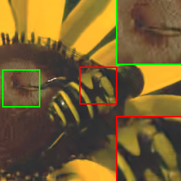
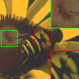
PSNR/SSIM	$\sigma=30$	31.65/0.8521	30.76/0.8496	27.86/0.6347
(a) GT	(b) NY	(c) CBM3D	(d) McWNNM	(e) SV-TV
	31.02/0.8213	32.47/0.8804	32.35/0.8809	32.57/0.8853
	(f) QLRMA	(g) QWSNM	(h) QWNNM	(i) Ours
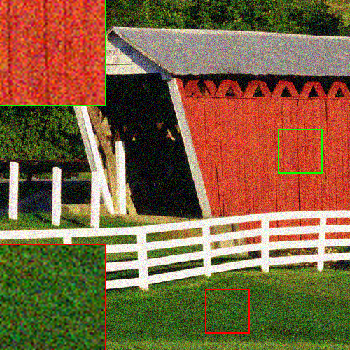
PSNR/SSIM	$\sigma=30$	29.86/0.8252	28.36/0.7768	27.77/0.7403
(a) GT	(b) NY	(c) CBM3D	(d) McWNNM	(e) SV-TV
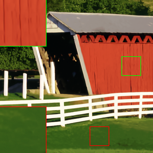
	29.10/0.7946	30.37/0.8326	30.33/0.8417	30.54/0.8469
	(f) QLRMA	(g) QWSNM	(h) QWNNM	(i) Ours

Figure 4: Comparison of visual results for color image denoising. The first two rows of images are from CSet12. The last two rows of images are from the McMaster dataset.

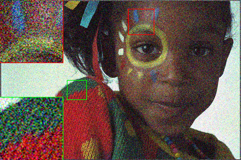
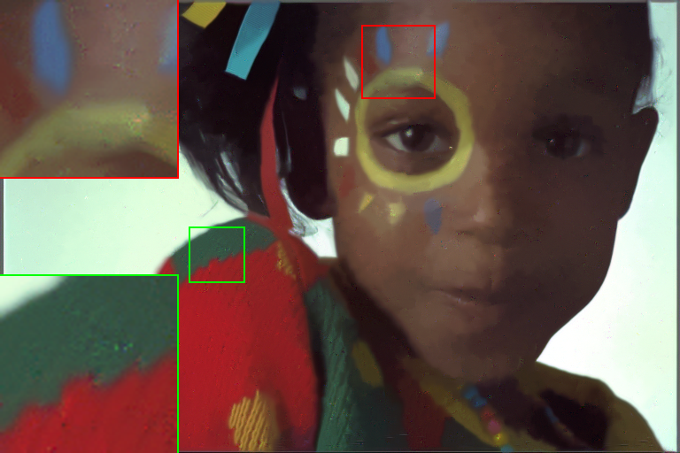
PSNR/SSIM	$\sigma=50$	30.22/0.8037	28.26/0.7495	26.02/0.5511
(a) GT	(b) NY	(c) CBM3D	(d) McWNNM	(e) SV-TV
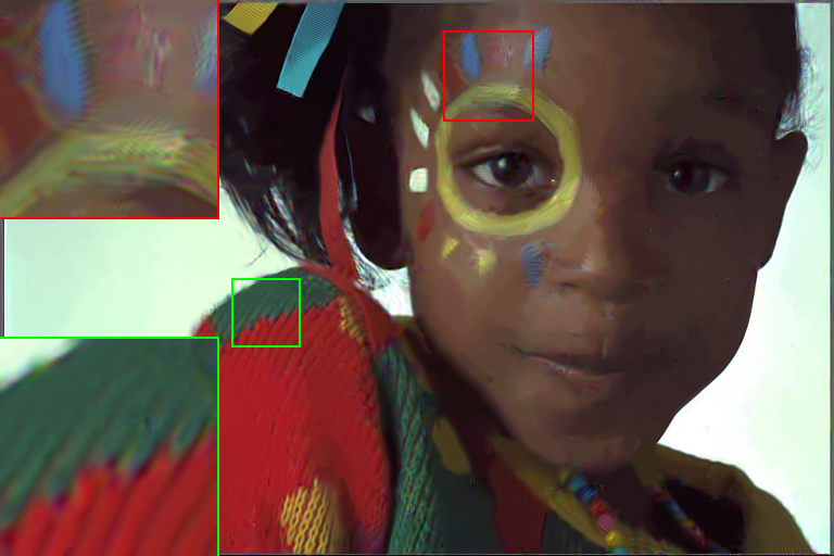
	29.44/0.7819	30.25/0.8014	30.34/0.8075	30.48/0.8091
	(f) QLRMA	(g) QWSNM	(h) QWNNM	(i) Ours
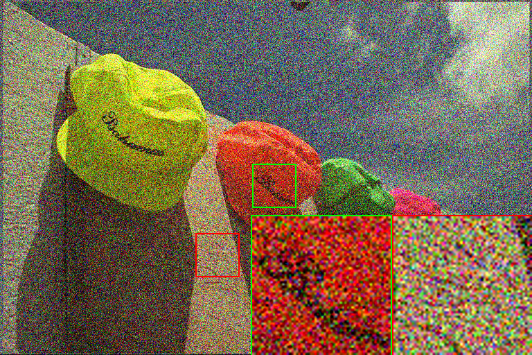
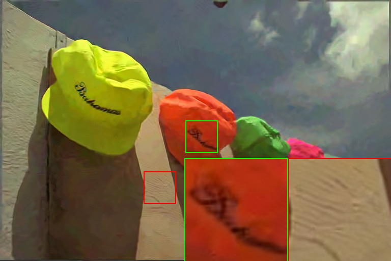
PSNR/SSIM	$\sigma=60$	30.52/0.8243	28.60/0.7630	25.07/0.4679
(a) GT	(b) NY	(c) CBM3D	(d) McWNNM	(e) SV-TV
	29.84/0.7994	30.52/0.8226	30.68/0.8278	30.82/0.8262
	(f) QLRMA	(g) QWSNM	(h) QWNNM	(i) Ours

Figure 5: Comparison of visual results for color image denoising. All images are from the Kodak dataset.

Table 1 illustrates the comparative results of color image denoising, showcasing the consistent state-of-the-art performance of the proposed QNMF across various datasets and noise levels. In general, the algorithm based on quaternion representation outperforms methods focusing on vectorization or color space transformation. Specifically, among quaternion representation-based approaches, QWNNM excels in handling high noise levels ($\sigma\geq 50$), while QWSNM is particularly effective for low to medium noise levels ($\sigma<50$). However, the proposed QNMF demonstrates robust performance across all noise levels.

The visual comparison of reconstructed images is depicted in Figures 4 and 5. SV-TV exhibits significant noise residuals. CBM3D, another color space transformation algorithm, generates numerous color artifacts, particularly noticeable in smooth image regions like the sky in the hat image (in Figure 5). These abrupt color changes stem from processing errors in smooth areas, which are highly discernible to the human eye, significantly influencing the perceived image quality. McWNNM, utilizing vectorization, produces fewer color artifacts but tends to oversmooth the image, leading to a loss of texture detail. Algorithms based on quaternion representation offer notable advantages in image color, attributed to the transformation and computation of inter-channel information facilitated by quaternion operations. Among these quaternion-based approaches, QNMF stands out for superior color and detail preservation, whereas both QWNNM and QWSNM suffer from excessive smoothing.

Table 2: Comparison of real denoising PSNR/SSIM values in cc, PolyU and SIDD datasets. The best results are shown in bold.

Real dataset	CBM3D [3]	McWNNM [16]	SV-TV [1]	QLRMA [21]	QWSNM [27]	QWNNM [22]	Ours
cc [38]	36.62/0.9379	35.99/0.9247	35.72/0.9348	36.29/0.9346	37.75/0.9555	37.69/0.9542	37.83/0.9566
PolyU [39]	37.93/0.9630	36.26/0.9513	37.15/0.9536	32.79/0.9115	37.88/0.9612	38.06/0.9622	38.10/0.9625
SIDD [40]	36.10/0.9093	34.40/0.8720	32.84/0.8147	32.49/0.7971	36.44/0.9137	36.49/0.9155	36.53/0.9166
Av.	36.88/0.9367	35.55/0.9160	35.24/0.9010	33.86/0.8811	37.36/0.9435	37.41/0.9440	37.49/0.9452

(a) GT	(b) NY	(c) CBM3D	(d) McWNNM	(e) SV-TV
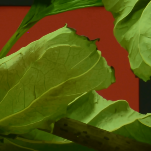
	(f) QLRMA	(g) QWSNM	(h) QWNNM	(i) Ours
(a) GT	(b) NY	(c) CBM3D	(d) McWNNM	(e) SV-TV
	(f) QLRMA	(g) QWSNM	(h) QWNNM	(i) Ours

Figure 6: Comparison of visual results for real color image denoising. The first two rows of images are from the cc dataset. The last two rows of images are from the SIDD dataset.

4.3 Real image denoising

In real image denoising, the algorithm setup remains consistent with the previous subsection. To address blind denoising, where the noise intensity level is unknown, we employed the noise intensity estimator proposed by [41] to estimate the $\sigma$ parameter for each algorithm.

Table 3: Comparison of debluring PSNR/SSIM values in CSet12 datasets. The best results are shown in bold.

Blur kernel	UB(9,9)/$\sigma=15$	GB(25,1.6)/$\sigma=15$	MB(20,60)/$\sigma=15$
SNSS [5]	20.02/0.5511	20.74/0.6438	19.95/0.5571
SV-TV [1]	22.57/0.6030	16.09/0.3634	19.77/0.4870
QD-SV-TV [4]	21.37/0.5551	22.75/0.6110	19.79/0.4944
QWSNM [27]	24.42/0.6879	26.15/0.7642	23.83/0.6687
QWNNM [25]	24.39/0.6862	26.02/0.7572	24.07/0.6819
Ours	24.45/0.6908	26.20/0.7665	24.19/0.6857

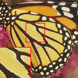
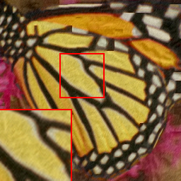
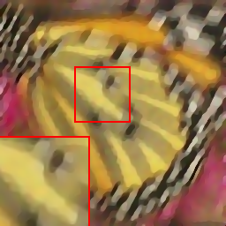
(a) GT	(b) Blur	(c) SNSS	(d) SV-TV
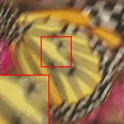
(e) QD-SV-TV	(f) QWSNM	(g) QWNNM	(h) Ours

Figure 7: Comparison of visual results of color image deblurring. The blurring kernel is MB(20,60)/$\sigma=15$.

Table 2 illustrates the results on three real image datasets, indicating that the proposed QNMF consistently performs well and achieves state-of-the-art results across all three datasets. This aligns with its performance in the denoising experiments discussed earlier. The visual comparison is presented in Figure 6. QNMF maintains its superiority, preserving more image details compared to other methods. For example, our algorithm better preserves leaf texture while effectively eliminating noise (see the first two rows of Figure 6).

4.4 Color image debluring

Taking color image deblurring as an example, we explored the potential of the proposed QNMF in low-level vision tasks. We considered three common blur kernels: a $9\times 9$ uniform kernel, a Gaussian kernel with a standard deviation of 1.6, and the motion kernel with a motion length of 20 and a motion angle of 60. All of these blurred images were affected by additive Gaussian noise with $\sigma=15$. Four algorithms, namely SV-TV [1], QWNNM [25], QWSNM [27], QD-SV-TV based on quaternion dictionary learning [4], and SNSS [5] based on gaussian mixture model, were used for comparison.

The parameters of the deblurring algorithm were set as follows: $\beta=8.5$, $\gamma=115$ for uniform blur; $\beta=7.5$, $\gamma=65$ for Gaussian blur; $\beta=7.5$, $\gamma=115$ for motion blur. 155 similar patches of $6\times 6$ were searched in the search window of 30. $\alpha$ was still set to 4.

Table 3 displays the reconstruction performance of the comparison algorithms for the three types of blurs. QWSNM shows superior performance under uniform and Gaussian blurs, while QWNNM excels at handling motion blur. The proposed QNMF consistently achieves state-of-the-art results across all three blurs. In Figure 7, a visual comparison between the proposed QNMF and state-of-the-art algorithms under motion blur is presented. The reconstruction outcomes of SV-TV and QD-SV-TV are unsatisfactory. Both QWNNM and QWSNM exhibit reconstruction artifacts, whereas the proposed QNMF demonstrates smooth reconstruction results. These findings underscore the remarkable potential of QNMF in addressing the color image linear inverse problem.

Table 4: Comparison of PSNR/SSIM values for color image matrix completion. The best results are marked in bold. The second best results are marked in red. Ours-G indicates processing on the global image and Ours-NNS indicates processing using image patches.

Miss rate	50%	60%	75%	80%
TRPCA [9]	24.26/ 0.7636	22.97/0.6901	20.70/0.5397	19.71/0.4745
QMC [42]	23.76/0.7594	22.75/ 0.6940	20.73/ 0.5504	19.82/ 0.4866
QWSNM [27]	25.47/0.6993	23.62/0.6124	19.14/0.3827	14.42/0.2097
QWNNM [25]	24.63/0.6577	22.80/0.5680	19.60/0.3942	17.04/0.2769
Ours-G	26.27/0.7594	24.36/0.6717	21.52/0.5083	20.37/0.4415
Ours-NNS	31.80/0.9397	29.85/0.9114	27.05/0.8512	23.81/0.7714

Table 5: Comparison of PSNR/SSIM values for color image random impulse noise removal. The best results are marked in bold. The second best results are marked in red. Ours-G indicates processing on the global image and Ours-NNS indicates processing using image patches.

Random rate	3%	5%	7%	10%
TRPCA [9]	29.56/ 0.9398	29.38/ 0.9343	29.14/0.9279	28.80/0.9170
QMC [42]	27.53/0.9119	27.37/0.9062	27.23/0.9004	26.99/ 0.8904
QWSNM [27]	24.32/0.7513	24.29/0.7489	24.25/0.7468	24.18/0.7438
QWNNM [25]	24.40/0.7582	24.39/0.7558	24.33/0.7534	24.28/0.7498
Ours-G	33.21/0.9462	32.07/0.9362	30.86/ 0.9164	29.34/0.8895
Ours-NNS	32.70/0.9093	30.98/0.8815	30.32/0.8617	29.58/0.8582

4.5 Matrix completion and Robust PCA

In this subsection, we evaluated the performance of QNMF in matrix completion and RPCA. For matrix completion, we assessed observation missing rates of 50%, 60%, 75%, and 80%. For RPCA, we added 3%, 5%, 7%, and 10% random impulse noise to the color images. We compared QNMF with tensor-based TRPCA [9], quaternion matrix completion (QMC) [42], QWNNM, and QWSNM. TRPCA, QMC, QWNNM, and QWSNM used global image computation. In contrast, QNMF utilized both NNS-based patch computation (Ours-NNS) and global image computation (Ours-G). For parameter settings, refer to [24, 26], with $\alpha$ set to 4.

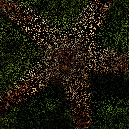
(a) GT	(b) Miss (80%)	(c) TRPCA	(d) QMC
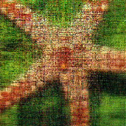
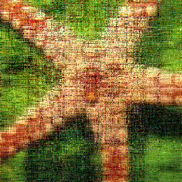
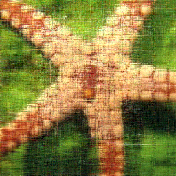
(e) QWSNM	(f) QWNNM	(g) Ours-G	(f) Ours-NNS

Figure 8: Comparison of visual results for color image matrix completion. The missing rate is 80%.

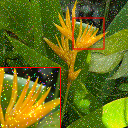
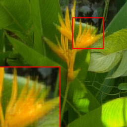
(a) GT	(b) NY (10%)	(c) TRPCA	(d) QMC
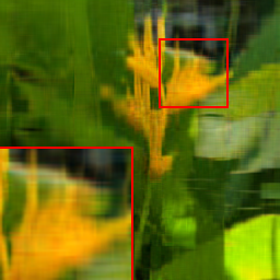
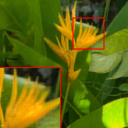
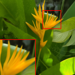
(e) QWSNM	(f) QWNNM	(g) Ours-G	(f) Ours-NNS

Figure 9: Comparison of visual results for random impulse noise removal from color images. The random rate is 10%.

Table 4 presents the numerical results of matrix completion, where QNMF-NNS achieves the best performance. QNMF-G ranks second in PSNR, while TRPCA and QMC perform well in SSIM. However, QWNNM and QWSNM, which excel in denoising and deblurring, exhibit subpar performance in matrix completion. Figure 8 illustrates the visual comparison of completion results for 80% missing data. Notably, the reconstructions by QWNNM and QWSNM exhibit significant noise, while those of TRPCA and QMC are overly smooth. QNMF-G stands out visually among global algorithms by preserving more details. QNMF-NNS leverages non-local self-similarity prior for superior results. Table 5 and Figure 9 present quantitative and qualitative RPCA results, respectively. The performance comparisons are similar to those in matrix completion, with QNMF-NNS not consistently optimal. QNMF-G outperforms QNMF-NNS particularly when random noise is minimal, as fewer pixel mutations interfere with the image, potentially leading to smoother outcomes with NNS utilization.

4.6 Ablation experiment

In the QNMF model (6), the parameter $\alpha$ is crucial. When $\alpha=0$, the QNMF model simplifies to the QNNM model. Setting $\alpha$ is critical because a value that is too large can truncate the shrinkage of singular values, making it ineffective. Therefore, $\alpha$ should be within a reasonable range to ensure effective singular value shrinkage. We evaluated the impact of $\alpha$ on the performance of the Gaussian denoising algorithm for various noise levels ($\sigma=5,20,40,60$). We tested $\alpha$ values of 0.5, 1, 2, 3, 4, 5, and 6, and plotted the performance curves in Figure 10. The trends for both PSNR and SSIM are similar with respect to $\alpha$. For $\alpha$ values between 0.5 and 3, the algorithm’s performance improves as $\alpha$ increases. However, for $\alpha$ values greater than 4, the performance begins to decline due to insufficient singular value shrinkage. Based on these observations, we typically set $\alpha=4$ in practical applications of the QNMF algorithm to balance performance and effective singular value shrinkage.

’

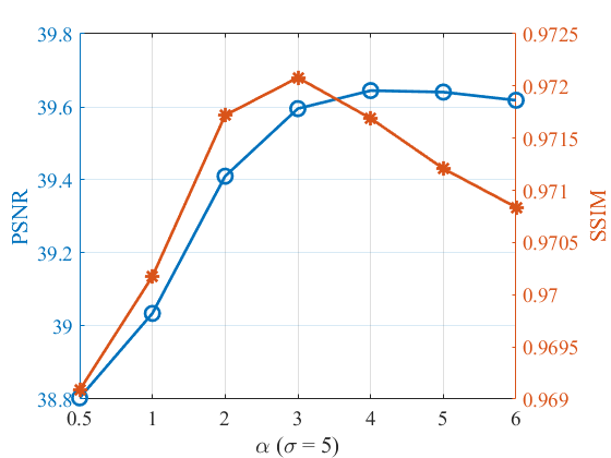
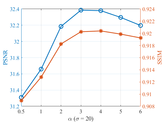
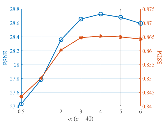
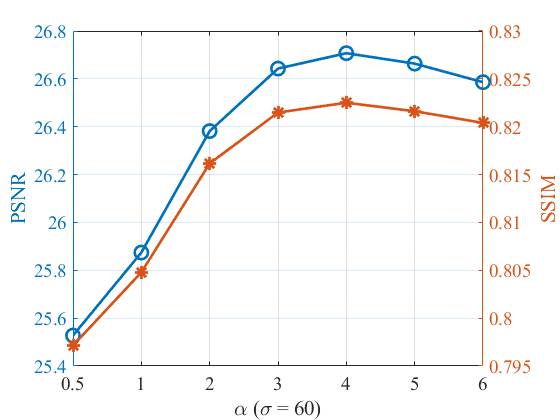
Figure 10: The effect of the value $\alpha$ on the denoising performance.

Table 6: The running time (s) of all algorithms on a PC with Intel (R) Core (TM) i7-13700KF 3.40 GHz and 64G RAM.

Denoising, $\sigma=40$
Size	CBM3D [3]	McWNNM [16]	SV-TV [1]	QLRMA [21]	QWSNM [27]	QWNNM [22]	Ours
256$\times$256	2.02	111.57	3.01	577.46	955.33	580.60	620.86
500$\times$500	7.38	460.51	11.53	2289.23	3379.72	2289.69	2423.98
Debluring, GB(25,1.6)/$\sigma=15$
Size	–	SNSS [5]	SV-TV [1]	QD-SV-TV [4]	QWSNM [27]	QWNNM [25]	Ours
256$\times$256	–	324.42	3.09	22.82	3959.28	3831.23	2154.88
Matrix completion, miss=80%
Size	–	–	TRPCA [9]	QMC [42]	QWSNM [27]	QWNNM [25]	Ours
256$\times$256	–	–	15.02	168.13	21.07	20.85	10.83

To demonstrate the computational complexity of different algorithms, we tested their runtimes on a PC with an Intel (R) Core (TM) i7-13700KF 3.40 GHz processor and 64GB RAM. The runtimes are shown in Table 6. CBM3D and SV-TV exhibit rapid runtimes, while low-rank class algorithms generally require longer runtimes. Notably, the proposed QNMF algorithm has an advantageous runtime among quaternion-based algorithms.

5 Limitation and Conclusion

Our comparison of runtimes reveals that algorithms utilizing the low-rank nature of images generally have longer runtimes. This is due to the fact that image rank often follows a long-tailed distribution, making direct use of low-rank priors less effective. To better exploit low-rank priors, similar image patches are typically combined with the self-similarity of images to form low-rank matrices. While this method improves results, it also increases computational complexity. Furthermore, algorithms based on quaternion algebra typically rely on QSVD, which is slower than SVD in the real number domain. These challenges highlight the need for future optimization efforts to enhance computational speed. Currently, deep learning algorithms are at the forefront of image reconstruction. Incorporating a priori knowledge from traditional algorithms into these learnable models will be a key area of focus moving forward.

In this paper, we investigate the quaternion nucleus norm minus Frobenius norm minimization (QNMF) problem and apply it to various image processing tasks. Initially, we introduce a strategy for solving the QNMF problem while minimizing the loss of F-norm fidelity, offering a closed-form solution. Subsequently, we extend the application of QNMF to address the color image linear inverse problem, matrix completion (MC), and robust principal component analysis (RPCA) using the ADMM framework. We provide rigorous proofs for all these methodologies to ensure their theoretical soundness. We validate the effectiveness of QNMF across various tasks, such as color image denoising, deblurring, inpainting, and random impulse noise removal. Experimental results confirm that the proposed method outperforms existing techniques, especially in preserving color fidelity and reducing artifacts. The ability to handle various rank components and the availability of closed-form solutions make QNMF a promising tool for future research in color image reconstruction and related applications. In the future, we will consider whether other quaternion hybrid norms can approximate the rank norm more accurately, such as the quaternion nuclear norm over Frobenius norm. Meanwhile, considering that QSVD has high computational complexity, QSVD-free quaternion methods will also be the focus of our future work.

Appendix

A. Proof of Theorem 3.2

Proof.

First, we prove that the sequence $\{\dot{\mathbf{\eta}}^{(k)}\}$ generated by Algorithm 1 is upper bounded.

$$||\dot{\mathbf{\eta}}^{(k+1)}||_{F}^{2} =||\dot{\mathbf{\eta}}^{(k)}+\beta^{(k)}(\dot{\mathbf{X}}^{(k+1)}-\dot{\mathbf{Z}}^{(k+1)})||_{F}^{2}$$ (36)

$$={\beta^{(k)}}^{2}||({\beta^{(k)}}^{-1}\dot{\mathbf{\eta}}^{(k)}+\dot{\mathbf{X}}^{(k+1)})-\dot{\mathbf{Z}}^{(k+1)}||_{F}^{2}$$

$$={\beta^{(k)}}^{2}||\dot{\mathbf{U}}^{(k)}\Sigma^{(k)}\mathbf{V}^{(k)\top}-\dot{\mathbf{U}}^{(k)}\Sigma^{(k)}_{\dot{\mathbf{Z}}}\mathbf{V}^{(k)\top}||_{F}^{2}$$

$$={\beta^{(k)}}^{2}\sum^{M}_{i=1}(\sigma^{(k)}_{i}-\sigma^{(k)}_{\dot{\mathbf{Z}},i})^{2}$$

$$\leq{\beta^{(k)}}^{2}\sum_{i=1}^{M}(\lambda/\beta^{(k)})^{2}$$

$$=\lambda^{2}M.$$

For the last inequality, if $\sigma^{(k)}_{i}\geq\lambda/\beta^{(k)}$, then $\sigma^{(k)}_{\dot{\mathbf{Z}},i}=\frac{||z||_{2}+\alpha\lambda/\beta^{(k)}}{||z||_{2}}\max(\sigma^{(k)}_{i}-\lambda/\beta^{(k)},0)$. Obviously $\sigma^{(k)}_{i}-\sigma^{(k)}_{\dot{\mathbf{Z}},i}\leq\lambda/\beta^{(k)}$ holds. If $\sigma^{(k)}_{i}<\lambda/\beta^{(k)}$, $\sigma^{(k)}_{i}-\sigma^{(k)}_{\dot{\mathbf{Z}},i}=\sigma^{(k)}_{i}<\lambda/\beta^{(k)}$. Hence, the sequence $\{\dot{\mathbf{\eta}}^{(k)}\}$ generated by Algorithm 1 is upper bounded.

Then, we prove that the sequence of Lagrange function $\{\mathcal{L}(\dot{\mathbf{X}}^{(k+1)},\dot{\mathbf{Z}}^{(k+1)},\dot{\mathbf{\eta}}^{(k+1)},\beta^{(k+1)})\}$ is also upper bounded. According to the update rule for $\dot{\mathbf{\eta}}^{(k)}$, it can be obtained

$$\mathcal{L}(\dot{\mathbf{X}}^{(k+1)},\dot{\mathbf{Z}}^{(k+1)},\dot{\mathbf{\eta}}^{(k+1)},\beta^{(k+1)})$$ (37)

$$~{}=\mathcal{L}(\dot{\mathbf{X}}^{(k+1)},\dot{\mathbf{Z}}^{(k+1)},\dot{\mathbf{\eta}}^{(k)},\beta^{(k)})+\langle{\dot{\mathbf{\eta}}^{(k+1)}-\dot{\mathbf{\eta}}^{(k)},\dot{\mathbf{X}}^{(k+1)}-\dot{\mathbf{Z}}^{(k+1)}}\rangle+\frac{\beta^{(k+1)}-\beta^{(k)}}{2}||\dot{\mathbf{X}}^{(k+1)}-\dot{\mathbf{Z}}^{(k+1)}||_{F}^{2}$$

$$~{}=\mathcal{L}(\dot{\mathbf{X}}^{(k+1)},\dot{\mathbf{Z}}^{(k+1)},\dot{\mathbf{\eta}}^{(k)},\beta^{(k)})+\langle{\dot{\mathbf{\eta}}^{(k+1)}-\dot{\mathbf{\eta}}^{(k)},\frac{\dot{\mathbf{\eta}}^{(k+1)}-\dot{\mathbf{\eta}}^{(k)}}{\beta^{(k)}}}\rangle+\frac{\beta^{(k+1)}-\beta^{(k)}}{2}||\frac{\dot{\mathbf{\eta}}^{(k+1)}-\dot{\mathbf{\eta}}^{(k)}}{\beta^{(k)}}||_{F}^{2}$$

$$~{}=\mathcal{L}(\dot{\mathbf{X}}^{(k+1)},\dot{\mathbf{Z}}^{(k+1)},\dot{\mathbf{\eta}}^{(k)},\beta^{(k)})+\frac{\beta^{(k+1)}+\beta^{(k)}}{2{\beta^{(k)}}^{2}}||\dot{\mathbf{\eta}}^{(k+1)}-\dot{\mathbf{\eta}}^{(k)}||_{F}^{2}.$$

Since $\{\dot{\mathbf{\eta}}^{(k)}\}$ is bounded, the sequence $\{\dot{\mathbf{\eta}}^{(k+1)}-\dot{\mathbf{\eta}}^{(k)}\}$ is also bounded. Suppose that the upper bound of the sequence $\{\dot{\mathbf{\eta}}^{(k+1)}-\dot{\mathbf{\eta}}^{(k)}\}$ is $M_{0}$, i.e., $\forall k\geq 0,||\dot{\mathbf{\eta}}^{(k+1)}-\dot{\mathbf{\eta}}^{(k)}||_{F}\leq M_{0}$. Meanwhile, the inequality $\mathcal{L}(\dot{\mathbf{X}}^{(k+1)},\dot{\mathbf{Z}}^{(k+1)},\dot{\mathbf{\eta}}^{(k)},\beta^{(k)})\leq\mathcal{L}(\dot{\mathbf{X}}^{(k)},\dot{\mathbf{Z}}^{(k)},\dot{\mathbf{\eta}}^{(k)},\beta^{(k)})$ always holds because $\dot{\mathbf{X}}$ and $\dot{\mathbf{Z}}$ are globally optimal solutions to the corresponding subproblems. Therefore, we have

$$\mathcal{L}(\dot{\mathbf{X}}^{(k+1)},\dot{\mathbf{Z}}^{(k+1)},\dot{\mathbf{\eta}}^{(k+1)},\beta^{(k+1)})$$ (38)

$$~{}\leq\mathcal{L}(\dot{\mathbf{X}}^{(k+1)},\dot{\mathbf{Z}}^{(k+1)},\dot{\mathbf{\eta}}^{(k)},\beta^{(k)})+\frac{\beta^{(k+1)}+\beta^{(k)}}{2{\beta^{(k)}}^{2}}M_{0}^{2}$$

$$~{}\leq\mathcal{L}(\dot{\mathbf{X}}^{(1)},\dot{\mathbf{Z}}^{(1)},\dot{\mathbf{\eta}}^{(0)},\beta^{(0)})+M_{0}^{2}\sum_{k=0}^{\infty}\frac{1+\mu}{2\beta^{(0)}\mu^{k}}$$

$$~{}\leq\mathcal{L}(\dot{\mathbf{X}}^{(1)},\dot{\mathbf{Z}}^{(1)},\dot{\mathbf{\eta}}^{(0)},\beta^{(0)})+\frac{M_{0}^{2}}{\beta^{(0)}}\sum_{k=0}^{\infty}\frac{1}{\mu^{k-1}}$$

$$~{}<-\infty.$$

Hence, $\{\mathcal{L}(\dot{\mathbf{X}}^{(k+1)},\dot{\mathbf{Z}}^{(k+1)},\dot{\mathbf{\eta}}^{(k+1)},\beta^{(k+1)})\}$ is upper bounded.

Next, we prove that the sequences $\{\dot{\mathbf{X}}^{(k)}$} and $\{\dot{\mathbf{Z}}^{(k)}\}$ are upper bounded. From formula (13), we have

$$\frac{\gamma}{2}||\dot{\mathbf{A}}\dot{\mathbf{X}}^{(k+1)}-\dot{\mathbf{Y}}||^{2}_{F}+\lambda(||\dot{\mathbf{Z}}^{(k+1)}||_{*}-\alpha||\dot{\mathbf{Z}}^{(k+1)}||_{F})$$ (39)

$$=\mathcal{L}(\dot{\mathbf{X}}^{(k+1)},\dot{\mathbf{Z}}^{(k+1)},\dot{\mathbf{\eta}}^{(k)},\beta^{(k)})-\langle{\dot{\mathbf{\eta}}^{(k)},\dot{\mathbf{X}}^{(k+1)}-\dot{\mathbf{Z}}^{(k+1)}}\rangle-\frac{\beta^{(k)}}{2}||\dot{\mathbf{X}}^{(k+1)}-\dot{\mathbf{Z}}^{(k+1)}||_{F}^{2}$$

$$=\mathcal{L}(\dot{\mathbf{X}}^{(k+1)},\dot{\mathbf{Z}}^{(k+1)},\dot{\mathbf{\eta}}^{(k)},\beta^{(k)})-\langle{\dot{\mathbf{\eta}}^{(k)},\frac{\dot{\mathbf{\eta}}^{(k+1)}-\dot{\mathbf{\eta}}^{(k)}}{\beta^{(k)}}}\rangle-\frac{\beta^{(k)}}{2}||\frac{\dot{\mathbf{\eta}}^{(k+1)}-\dot{\mathbf{\eta}}^{(k)}}{\beta^{(k)}}||_{F}^{2}$$

$$=\mathcal{L}(\dot{\mathbf{X}}^{(k+1)},\dot{\mathbf{Z}}^{(k+1)},\dot{\mathbf{\eta}}^{(k)},\beta^{(k)})+\frac{||\dot{\mathbf{\eta}}^{(k)}||_{F}^{2}-||\dot{\mathbf{\eta}}^{(k+1)}||_{F}^{2}}{2\beta^{(k)}}.$$

From this, we get that $\{\dot{\mathbf{A}}\dot{\mathbf{X}}^{(k)}-\dot{\mathbf{Y}}\}$ and $\{\dot{\mathbf{Z}}^{(k)}\}$ are upper bounded. Since $\dot{\mathbf{\eta}}^{(k+1)}=\dot{\mathbf{\eta}}^{(k)}+\beta^{(k)}(\dot{\mathbf{X}}^{(k+1)}-\dot{\mathbf{Z}}^{(k+1)})$, $\{\dot{\mathbf{X}}^{(k)}\}$ is also upper bounded. Thus, there exists at least one accumulation point for $\{\dot{\mathbf{X}}^{(k)},\dot{\mathbf{Z}}^{(k)}\}$. Further, we can get

$$\lim_{k\rightarrow+\infty}||\dot{\mathbf{X}}^{(k+1)}-\dot{\mathbf{Z}}^{(k+1)}||_{F} =\lim_{k\rightarrow+\infty}\frac{1}{\beta^{(k)}}||\dot{\mathbf{\eta}}^{(k+1)}-\dot{\mathbf{\eta}}^{(k)}||_{F}$$ (40)

$$=0,$$

and that the accumulation point is a feasible solution to the objective function. Thus, the first equation in (18) is proved.

Finally, we demonstrate that the change in the sequences $\{\dot{\mathbf{X}}^{(k)}\}$ and $\{\dot{\mathbf{Z}}^{(k)}\}$ converges to 0 with iteration. By $\dot{\mathbf{X}}^{(k)}=\frac{1}{\beta^{(k-1)}}(\dot{\mathbf{\eta}}^{(k)}-\dot{\mathbf{\eta}}^{(k-1)})+\dot{\mathbf{Z}}^{(k)}$, we get

$$\lim_{k\rightarrow+\infty}||\dot{\mathbf{X}}^{(k+1)}-\dot{\mathbf{X}}^{(k)}||_{F}$$ (41)

$$~{}=\lim_{k\rightarrow+\infty}||(\gamma\dot{\mathbf{A}}^{*}\dot{\mathbf{A}}+\beta^{(k)}\dot{\mathbf{I}})^{-1}(\gamma\dot{\mathbf{A}}^{*}\dot{\mathbf{Y}}+\beta^{(k)}\dot{\mathbf{Z}}^{(k)}-\dot{\mathbf{\eta}}^{(k)})-\frac{1}{\beta^{(k-1)}}(\dot{\mathbf{\eta}}^{(k)}-\dot{\mathbf{\eta}}^{(k-1)})-\dot{\mathbf{Z}}^{(k)}||_{F}$$

$$~{}=\lim_{k\rightarrow+\infty}||(\gamma\dot{\mathbf{A}}^{*}\dot{\mathbf{A}}+\beta^{(k)}\dot{\mathbf{I}})^{-1}(\gamma\dot{\mathbf{A}}^{*}\dot{\mathbf{Y}}-\gamma\dot{\mathbf{A}}^{*}\dot{\mathbf{A}}\dot{\mathbf{Z}}^{(k)}-\dot{\mathbf{\eta}}^{(k)})-\frac{1}{\beta^{(k-1)}}(\dot{\mathbf{\eta}}^{(k)}-\dot{\mathbf{\eta}}^{(k-1)})||_{F}$$

$$~{}\leq\lim_{k\rightarrow+\infty}||(\gamma\dot{\mathbf{A}}^{*}\dot{\mathbf{A}}+\beta^{(k)}\dot{\mathbf{I}})^{-1}(\gamma\dot{\mathbf{A}}^{*}\dot{\mathbf{Y}}-\gamma\dot{\mathbf{A}}^{*}\dot{\mathbf{A}}\dot{\mathbf{Z}}^{(k)}-\dot{\mathbf{\eta}}^{(k)})||_{F}+\frac{1}{\beta^{(k-1)}}||\dot{\mathbf{\eta}}^{(k)}-\dot{\mathbf{\eta}}^{(k-1)}||_{F}$$

$$~{}=0.$$

Similarly, we get

$$\lim_{k\rightarrow+\infty}||\dot{\mathbf{Z}}^{(k+1)}-\dot{\mathbf{Z}}^{(k)}||_{F}$$ (42)

$$~{}=\lim_{k\rightarrow+\infty}||\frac{1}{\beta^{(k)}}(\dot{\mathbf{\eta}}^{(k)}-\dot{\mathbf{\eta}}^{(k+1)})+\dot{\mathbf{X}}^{(k+1)}-\dot{\mathbf{Z}}^{(k)}||_{F}$$

$$~{}=\lim_{k\rightarrow+\infty}||\dot{\mathbf{X}}^{(k)}+\frac{1}{\beta^{(k-1)}}\dot{\mathbf{\eta}}^{(k-1)}-\dot{\mathbf{Z}}^{(k)}+\dot{\mathbf{X}}^{(k+1)}-\dot{\mathbf{X}}^{(k)}+\frac{1}{\beta^{(k)}}(\dot{\mathbf{\eta}}^{(k)}-\dot{\mathbf{\eta}}^{(k+1)})-\frac{1}{\beta^{(k-1)}}\dot{\mathbf{\eta}}^{(k-1)}||_{F}$$

$$~{}\leq\lim_{k\rightarrow+\infty}||\dot{\mathbf{X}}^{(k)}+\frac{1}{\beta^{(k-1)}}\dot{\mathbf{\eta}}^{(k-1)}-\dot{\mathbf{Z}}^{(k)}||_{F}+||\dot{\mathbf{X}}^{(k+1)}-\dot{\mathbf{X}}^{(k)}||_{F}+||\frac{1}{\beta^{(k)}}(\dot{\mathbf{\eta}}^{(k)}-\dot{\mathbf{\eta}}^{(k+1)})-\frac{1}{\beta^{(k-1)}}\dot{\mathbf{\eta}}^{(k-1)}||_{F}$$

$$~{}=\lim_{k\rightarrow+\infty}||\dot{\mathbf{X}}^{(k)}+\frac{1}{\beta^{(k-1)}}\dot{\mathbf{\eta}}^{(k-1)}-\dot{\mathbf{Z}}^{(k)}||_{F}+||\dot{\mathbf{X}}^{(k+1)}-\dot{\mathbf{X}}^{(k)}||_{F}+||\frac{1}{\beta^{(k)}}(\dot{\mathbf{\eta}}^{(k+1)}-\dot{\mathbf{\eta}}^{(k)})||_{F}+||\frac{1}{\beta^{(k-1)}}\dot{\mathbf{\eta}}^{(k-1)}||_{F}$$

$$~{}=\lim_{k\rightarrow+\infty}||\frac{1}{\beta^{(k-1)}}\dot{\mathbf{\eta}}^{(k)}||_{F}+||\dot{\mathbf{X}}^{(k+1)}-\dot{\mathbf{X}}^{(k)}||_{F}+||\dot{\mathbf{X}}^{(k+1)}-\dot{\mathbf{Z}}^{(k+1)}||_{F}+||\frac{1}{\beta^{(k-1)}}\dot{\mathbf{\eta}}^{(k-1)}||_{F}$$

$$~{}=0.$$

∎

Supplementary Material

B. Proof of Theorem 3.4

Proof.

First, we prove that the sequence $\{\dot{\mathbf{\eta}}^{(k)}\}$ generated by Algorithm 3 is upper bounded.

$$||\dot{\mathbf{\eta}}^{(k+1)}||_{F}^{2} =||\dot{\mathbf{\eta}}^{(k)}+\beta^{(k)}(\dot{\mathbf{Y}}-\dot{\mathbf{X}}^{(k+1)}-\dot{\mathbf{Z}}^{(k+1)})||_{F}^{2}$$ (43)

$$={\beta^{(k)}}^{2}||({\beta^{(k)}}^{-1}\dot{\mathbf{\eta}}^{(k)}+\dot{\mathbf{Y}}-\dot{\mathbf{Z}}^{(k+1)})-\dot{\mathbf{X}}^{(k+1)}||_{F}^{2}$$

$$={\beta^{(k)}}^{2}||\dot{\mathbf{U}}^{(k)}\Sigma^{(k)}\mathbf{V}^{(k)\top}-\dot{\mathbf{U}}^{(k)}\Sigma^{(k)}_{\dot{\mathbf{X}}}\mathbf{V}^{(k)\top}||_{F}^{2}$$

$$={\beta^{(k)}}^{2}\sum^{M}_{i=1}(\sigma^{(k)}_{i}-\sigma^{(k)}_{\dot{\mathbf{X}},i})^{2}$$

$$\leq{\beta^{(k)}}^{2}\sum_{i=1}^{M}(\lambda/\beta^{(k)})^{2}$$

$$=\lambda^{2}M.$$

For the last inequality, if $\sigma^{(k)}_{i}\geq\lambda/\beta^{(k)}$, then $\sigma^{(k)}_{\dot{\mathbf{X}},i}=\frac{||x||_{2}+\alpha\lambda/\beta^{(k)}}{||x||_{2}}\max(\sigma^{(k)}_{i}-\lambda/\beta^{(k)},0)$. Obviously $\sigma^{(k)}_{i}-\sigma^{(k)}_{\dot{\mathbf{X}},i}\leq\lambda/\beta^{(k)}$ holds. If $\sigma^{(k)}_{i}<\lambda/\beta^{(k)}$, $\sigma^{(k)}_{i}-\sigma^{(k)}_{\dot{\mathbf{X}},i}=\sigma^{(k)}_{i}<\lambda/\beta^{(k)}$. Hence, the sequence $\{\dot{\mathbf{\eta}}^{(k)}\}$ generated by Algorithm 3 is upper bounded.

Then, we prove that the sequence of Lagrange function $\{\mathcal{L}(\dot{\mathbf{X}}^{(k+1)},\dot{\mathbf{Z}}^{(k+1)},\dot{\mathbf{\eta}}^{(k+1)},\beta^{(k+1)})\}$ is also upper bounded. According to the update rule for $\dot{\mathbf{\eta}}^{(k)}$, it can be obtained

$$\mathcal{L}(\dot{\mathbf{X}}^{(k+1)},\dot{\mathbf{Z}}^{(k+1)},\dot{\mathbf{\eta}}^{(k+1)},\beta^{(k+1)})$$ (44)

$$~{}=\mathcal{L}(\dot{\mathbf{X}}^{(k+1)},\dot{\mathbf{Z}}^{(k+1)},\dot{\mathbf{\eta}}^{(k)},\beta^{(k)})+\langle{\dot{\mathbf{\eta}}^{(k+1)}-\dot{\mathbf{\eta}}^{(k)},\dot{\mathbf{Y}}-\dot{\mathbf{X}}^{(k+1)}-\dot{\mathbf{Z}}^{(k+1)}}\rangle+\frac{\beta^{(k+1)}-\beta^{(k)}}{2}||\dot{\mathbf{Y}}-\dot{\mathbf{X}}^{(k+1)}-\dot{\mathbf{Z}}^{(k+1)}||_{F}^{2}$$

$$~{}=\mathcal{L}(\dot{\mathbf{X}}^{(k+1)},\dot{\mathbf{Z}}^{(k+1)},\dot{\mathbf{\eta}}^{(k)},\beta^{(k)})+\langle{\dot{\mathbf{\eta}}^{(k+1)}-\dot{\mathbf{\eta}}^{(k)},\frac{\dot{\mathbf{\eta}}^{(k+1)}-\dot{\mathbf{\eta}}^{(k)}}{\beta^{(k)}}}\rangle+\frac{\beta^{(k+1)}-\beta^{(k)}}{2}||\frac{\dot{\mathbf{\eta}}^{(k+1)}-\dot{\mathbf{\eta}}^{(k)}}{\beta^{(k)}}||_{F}^{2}$$

$$~{}=\mathcal{L}(\dot{\mathbf{X}}^{(k+1)},\dot{\mathbf{Z}}^{(k+1)},\dot{\mathbf{\eta}}^{(k)},\beta^{(k)})+\frac{\beta^{(k+1)}+\beta^{(k)}}{2{\beta^{(k)}}^{2}}||\dot{\mathbf{\eta}}^{(k+1)}-\dot{\mathbf{\eta}}^{(k)}||_{F}^{2}.$$

Since $\{\dot{\mathbf{\eta}}^{(k)}\}$ is bounded, the sequence $\{\dot{\mathbf{\eta}}^{(k+1)}-\dot{\mathbf{\eta}}^{(k)}\}$ is also bounded. Suppose that the upper bound of the sequence $\{\dot{\mathbf{\eta}}^{(k+1)}-\dot{\mathbf{\eta}}^{(k)}\}$ is $M_{1}$, i.e., $\forall k\geq 0,||\dot{\mathbf{\eta}}^{(k+1)}-\dot{\mathbf{\eta}}^{(k)}||_{F}\leq M_{1}$. Meanwhile, the inequality $\mathcal{L}(\dot{\mathbf{X}}^{(k+1)},\dot{\mathbf{Z}}^{(k+1)},\dot{\mathbf{\eta}}^{(k)},\beta^{(k)})\leq\mathcal{L}(\dot{\mathbf{X}}^{(k)},\dot{\mathbf{Z}}^{(k)},\dot{\mathbf{\eta}}^{(k)},\beta^{(k)})$ always holds because $\dot{\mathbf{X}}$ and $\dot{\mathbf{Z}}$ are globally optimal solutions to the corresponding subproblems. Therefore, we have

$$\mathcal{L}(\dot{\mathbf{X}}^{(k+1)},\dot{\mathbf{Z}}^{(k+1)},\dot{\mathbf{\eta}}^{(k+1)},\beta^{(k+1)})$$

$$~{}\leq\mathcal{L}(\dot{\mathbf{X}}^{(k+1)},\dot{\mathbf{Z}}^{(k+1)},\dot{\mathbf{\eta}}^{(k)},\beta^{(k)})+\frac{\beta^{(k+1)}+\beta^{(k)}}{2{\beta^{(k)}}^{2}}M_{1}^{2}$$

$$~{}\leq\mathcal{L}(\dot{\mathbf{X}}^{(1)},\dot{\mathbf{Z}}^{(1)},\dot{\mathbf{\eta}}^{(0)},\beta^{(0)})+M_{1}^{2}\sum_{k=0}^{\infty}\frac{1+\mu}{2\beta^{(0)}\mu^{k}}$$ (45)

$$~{}\leq\mathcal{L}(\dot{\mathbf{X}}^{(1)},\dot{\mathbf{Z}}^{(1)},\dot{\mathbf{\eta}}^{(0)},\beta^{(0)})+\frac{M_{1}^{2}}{\beta^{(0)}}\sum_{k=0}^{\infty}\frac{1}{\mu^{k-1}}$$

$$~{}<-\infty.$$

Hence, $\{\mathcal{L}(\dot{\mathbf{X}}^{(k+1)},\dot{\mathbf{Z}}^{(k+1)},\dot{\mathbf{\eta}}^{(k+1)},\beta^{(k+1)})\}$ is upper bounded.

Next, we prove that the sequences $\{\dot{\mathbf{X}}^{(k)}$} and $\{\dot{\mathbf{Z}}^{(k)}\}$ are upper bounded.

$$\lambda(||\dot{\mathbf{X}}^{(k+1)}||_{*}-\alpha||\dot{\mathbf{X}}^{(k+1)}||_{F})+\rho||\dot{\mathbf{Z}}^{(k+1)}||_{1}$$ (46)

$$=\mathcal{L}(\dot{\mathbf{X}}^{(k+1)},\dot{\mathbf{Z}}^{(k+1)},\dot{\mathbf{\eta}}^{(k)},\beta^{(k)})-\langle{\dot{\mathbf{\eta}}^{(k)},\dot{\mathbf{Y}}-\dot{\mathbf{X}}^{(k+1)}-\dot{\mathbf{Z}}^{(k+1)}}\rangle-\frac{\beta^{(k)}}{2}||\dot{\mathbf{Y}}-\dot{\mathbf{X}}^{(k+1)}-\dot{\mathbf{Z}}^{(k+1)}||_{F}^{2}$$

$$=\mathcal{L}(\dot{\mathbf{X}}^{(k+1)},\dot{\mathbf{Z}}^{(k+1)},\dot{\mathbf{\eta}}^{(k)},\beta^{(k)})-\langle{\dot{\mathbf{\eta}}^{(k)},\frac{\dot{\mathbf{\eta}}^{(k+1)}-\dot{\mathbf{\eta}}^{(k)}}{\beta^{(k)}}}\rangle-\frac{\beta^{(k)}}{2}||\frac{\dot{\mathbf{\eta}}^{(k+1)}-\dot{\mathbf{\eta}}^{(k)}}{\beta^{(k)}}||_{F}^{2}$$

$$=\mathcal{L}(\dot{\mathbf{X}}^{(k+1)},\dot{\mathbf{Z}}^{(k+1)},\dot{\mathbf{\eta}}^{(k)},\beta^{(k)})+\frac{||\dot{\mathbf{\eta}}^{(k)}||_{F}^{2}-||\dot{\mathbf{\eta}}^{(k+1)}||_{F}^{2}}{2\beta^{(k)}}.$$

From this, we get that $\{\dot{\mathbf{X}}^{(k)}\}$ and $\{\dot{\mathbf{Z}}^{(k)}\}$ are upper bounded. Thus, there exists at least one accumulation point for $\{\dot{\mathbf{X}}^{(k)},\dot{\mathbf{Z}}^{(k)}\}$. Further, we can get

$$\lim_{k\rightarrow+\infty}||\dot{\mathbf{Y}}-\dot{\mathbf{X}}^{(k+1)}-\dot{\mathbf{Z}}^{(k+1)}||_{F} =\lim_{k\rightarrow+\infty}\frac{1}{\beta^{(k)}}||\dot{\mathbf{\eta}}^{(k+1)}-\dot{\mathbf{\eta}}^{(k)}||_{F}$$ (47)

$$=0,$$

and that the accumulation point is a feasible solution to the objective function. Thus, the first equation in (32) is proved.

Finally, we demonstrate that the change in the sequences $\{\dot{\mathbf{X}}^{(k)}\}$ and $\{\dot{\mathbf{Z}}^{(k)}\}$ converges to 0 with iteration. For $\dot{\mathbf{Z}}$ subproblem, by $\dot{\mathbf{Z}}^{(k)}=\dot{\mathbf{Y}}-\dot{\mathbf{X}}^{(k)}+\frac{\dot{\mathbf{\eta}}^{(k-1)}-\dot{\mathbf{\eta}}^{(k)}}{\beta^{(k-1)}}$, we get

$$\lim_{k\rightarrow+\infty}||\dot{\mathbf{Z}}^{(k+1)}-\dot{\mathbf{Z}}^{(k)}||_{F}$$ (48)

$$~{}=\lim_{k\rightarrow+\infty}||\mathcal{S}_{\frac{\rho}{\beta^{(k)}}}(\dot{\mathbf{Y}}-\dot{\mathbf{X}}^{(k)}+\frac{\dot{\mathbf{\eta}}^{(k)}}{\beta^{(k)}})-(\dot{\mathbf{Y}}-\dot{\mathbf{X}}^{(k)}+\frac{\dot{\mathbf{\eta}}^{(k)}}{\beta^{(k)}})+(\frac{\dot{\mathbf{\eta}}^{(k)}}{\beta^{(k-1)}}-\frac{\dot{\mathbf{\eta}}^{(k-1)}}{\beta^{(k-1)}}+\frac{\dot{\mathbf{\eta}}^{(k)}}{\beta^{(k)}})||_{F}$$

$$~{}\leq\lim_{k\rightarrow+\infty}||\mathcal{S}_{\frac{\rho}{\beta^{(k)}}}(\dot{\mathbf{Y}}-\dot{\mathbf{X}}^{(k)}+\frac{\dot{\mathbf{\eta}}^{(k)}}{\beta^{(k)}})-(\dot{\mathbf{Y}}-\dot{\mathbf{X}}^{(k)}+\frac{\dot{\mathbf{\eta}}^{(k)}}{\beta^{(k)}})||_{F}+||\frac{\dot{\mathbf{\eta}}^{(k)}}{\beta^{(k-1)}}-\frac{\dot{\mathbf{\eta}}^{(k-1)}}{\beta^{(k-1)}}+\frac{\dot{\mathbf{\eta}}^{(k)}}{\beta^{(k)}}||_{F}$$

$$~{}\leq\lim_{k\rightarrow+\infty}\frac{\rho\sqrt{mn}}{\beta^{(k)}}+||\frac{(\mu+1)\dot{\mathbf{\eta}}^{(k)}-\mu\dot{\mathbf{\eta}}^{(k-1)}}{\beta^{(k)}}||_{F}$$

$$~{}=0,$$

where $\mathcal{S}_{\frac{\rho}{\beta^{(k)}}}$ is the soft-threshold operation with parameter $\frac{\rho}{\beta^{(k)}}$, $m$ and $n$ are the size of $\dot{\mathbf{Y}}$.

Similarly, we prove that $\lim_{k\rightarrow+\infty}||\dot{\mathbf{X}}^{(k+1)}-\dot{\mathbf{X}}^{(k)}||_{F}=0$. By Algorithm 3, we get

$$\dot{\mathbf{X}}^{(k+1)}=\dot{\mathbf{Y}}-\dot{\mathbf{Z}}^{(k+1)}+\frac{\dot{\mathbf{\eta}}^{(k)}-\dot{\mathbf{\eta}}^{(k+1)}}{\beta^{(k)}},$$

$$\dot{\mathbf{X}}^{(k)}=\dot{\mathbf{U}}^{(k-1)}\mathcal{S}^{\mathrm{QNMF}}_{\frac{\lambda}{\beta^{(k-1)}}}(\Sigma^{(k-1)})\dot{\mathbf{V}}^{(k-1)\top},$$

where $\dot{\mathbf{U}}^{(k-1)}\Sigma^{(k-1)}\dot{\mathbf{V}}^{(k-1)\top}$ is the QSVD of $\dot{\mathbf{Y}}-\dot{\mathbf{Z}}^{(k)}+\frac{\dot{\mathbf{\eta}^{(k-1)}}}{\beta^{(k-1)}}$, $\mathcal{S}^{\mathrm{QNMF}}_{\frac{\lambda}{\beta^{(k-1)}}}$ is the QNMF closed solution operator provided by Theorem III.1 and Eq. (8). Then, we have

$$\lim_{k\rightarrow+\infty}||\dot{\mathbf{X}}^{(k+1)}-\dot{\mathbf{X}}^{(k)}||_{F}$$ (49)

$$~{}=\lim_{k\rightarrow+\infty}||\dot{\mathbf{Y}}-\dot{\mathbf{Z}}^{(k+1)}+\frac{\dot{\mathbf{\eta}}^{(k)}-\dot{\mathbf{\eta}}^{(k+1)}}{\beta^{(k)}}-\dot{\mathbf{X}}^{(k)}||_{F}$$

$$~{}=\lim_{k\rightarrow+\infty}||\dot{\mathbf{Y}}-\dot{\mathbf{Z}}^{(k+1)}+\frac{\dot{\mathbf{\eta}}^{(k)}-\dot{\mathbf{\eta}}^{(k+1)}}{\beta^{(k)}}-\dot{\mathbf{X}}^{(k)}+(\dot{\mathbf{Z}}^{(k)}+\frac{\dot{\mathbf{\eta}}^{(k-1)}}{\beta^{(k-1)}})-(\dot{\mathbf{Z}}^{(k)}+\frac{\dot{\mathbf{\eta}}^{(k-1)}}{\beta^{(k-1)}})||_{F}$$

$$~{}\leq\lim_{k\rightarrow+\infty}||(\dot{\mathbf{Y}}-\dot{\mathbf{Z}}^{(k)}+\frac{\dot{\mathbf{\eta}}^{(k-1)}}{\beta^{(k-1)}})-\dot{\mathbf{X}}^{(k)}||_{F}+||\dot{\mathbf{Z}}^{(k)}-\dot{\mathbf{Z}}^{(k+1)}||_{F}+||\frac{\dot{\mathbf{\eta}}^{(k)}-\dot{\mathbf{\eta}}^{(k+1)}}{\beta^{(k)}}-\frac{\dot{\mathbf{\eta}}^{(k-1)}}{\beta^{(k-1)}}||_{F}$$

$$~{}=\lim_{k\rightarrow+\infty}||\Sigma^{(k-1)}-\mathcal{S}^{\mathrm{QNMF}}_{\frac{\lambda}{\beta^{(k-1)}}}(\Sigma^{(k-1)})||_{F}+||\dot{\mathbf{Z}}^{(k)}-\dot{\mathbf{Z}}^{(k+1)}||_{F}+||\frac{\dot{\mathbf{\eta}}^{(k)}-(\mu+1)\dot{\mathbf{\eta}}^{(k+1)}}{\beta^{(k)}}||_{F}$$

$$~{}\leq\lim_{k\rightarrow+\infty}\frac{\lambda\sqrt{mn}}{\beta^{(k-1)}}+||\dot{\mathbf{Z}}^{(k)}-\dot{\mathbf{Z}}^{(k+1)}||_{F}+||\frac{\dot{\mathbf{\eta}}^{(k)}-(\mu+1)\dot{\mathbf{\eta}}^{(k+1)}}{\beta^{(k)}}||_{F}$$

$$~{}=0$$

∎

References

- Jia et al. [2019] Z. Jia, M. K. Ng, W. Wang, Color image restoration by saturation-value total variation, SIAM J. Imaging Sci. 12 (2019) 972–1000. doi:10.1137/18M1230451.
- Dabov et al. [2007a] K. Dabov, A. Foi, V. Katkovnik, K. Egiazarian, Image denoising by sparse 3-d transform-domain collaborative filtering, IEEE Trans. Image Process. 16 (2007a) 2080–2095. doi:10.1109/TIP.2007.901238.
- Dabov et al. [2007b] K. Dabov, A. Foi, V. Katkovnik, K. Egiazarian, Color image denoising via sparse 3d collaborative filtering with grouping constraint in luminance-chrominance space, in: Proc. IEEE Int. Conf. Image Process., volume 1, IEEE, 2007b, pp. I–313. doi:10.1109/ICIP.2007.4378954.
- Huang et al. [2021] C. Huang, M. K. Ng, T. Wu, T. Zeng, Quaternion-based dictionary learning and saturation-value total variation regularization for color image restoration, IEEE Trans. Multimedia 24 (2021) 3769–3781. doi:10.1109/TMM.2021.3107162.
- Zha et al. [2020] Z. Zha, X. Yuan, J. Zhou, C. Zhu, B. Wen, Image restoration via simultaneous nonlocal self-similarity priors, IEEE Trans. Image Process. 29 (2020) 8561–8576. doi:10.1109/TIP.2020.3015545.
- Gu et al. [2014] S. Gu, L. Zhang, W. Zuo, X. Feng, Weighted nuclear norm minimization with application to image denoising, in: Proc. IEEE Conf. Comput. Vis. Pattern Recognit., 2014, pp. 2862–2869. doi:10.1109/CVPR.2014.366.
- Guo et al. [2022] J. Guo, Y. Guo, Q. Jin, M. Kwok-Po Ng, S. Wang, Gaussian patch mixture model guided low-rank covariance matrix minimization for image denoising, SIAM J. Imaging Sci. 15 (2022) 1601–1622. doi:10.1137/21M1454262.
- Jiang et al. [2023] W. Jiang, J. Zhang, C. Zhang, L. Wang, H. Qi, Robust low tubal rank tensor completion via factor tensor norm minimization, Pattern Recognit. 135 (2023) 109169. doi:10.1016/j.patcog.2022.109169.
- Yang et al. [2020] J.-H. Yang, X.-L. Zhao, T.-Y. Ji, T.-H. Ma, T.-Z. Huang, Low-rank tensor train for tensor robust principal component analysis, Appl. Math. Comput. 367 (2020) 124783. doi:10.1016/j.amc.2019.124783.
- Zhang et al. [2017] K. Zhang, W. Zuo, Y. Chen, D. Meng, L. Zhang, Beyond a gaussian denoiser: Residual learning of deep cnn for image denoising, IEEE Trans. Image Process. 26 (2017) 3142–3155. doi:10.1109/TIP.2017.2662206.
- Guo et al. [2021] Y. Guo, A. Davy, G. Facciolo, J.-M. Morel, Q. Jin, Fast, nonlocal and neural: A lightweight high quality solution to image denoising, IEEE Signal Processing Letters 28 (2021) 1515–1519. doi:10.1109/LSP.2021.3099963.
- Hurault et al. [2018] S. Hurault, T. Ehret, P. Arias, Epll: an image denoising method using a gaussian mixture model learned on a large set of patches, Image Processing On Line 8 (2018) 465–489. doi:10.5201/ipol.2018.242.
- Guo et al. [2024] Y. Guo, Q. Jin, J.-M. Morel, G. Facciolo, How to best combine demosaicing and denoising?, Inverse Probl. Imaging 18 (2024) 571–599. doi:10.3934/ipi.2023044.
- Kong and Yang [2019] Z. Kong, X. Yang, Color image and multispectral image denoising using block diagonal representation, IEEE Trans. Image Process. 28 (2019) 4247–4259. doi:10.1109/TIP.2019.2907478.
- Miao et al. [2020] J. Miao, K. I. Kou, W. Liu, Low-rank quaternion tensor completion for recovering color videos and images, Pattern Recognit. 107 (2020) 107505. doi:10.1016/j.patcog.2020.107505.
- Xu et al. [2017] J. Xu, L. Zhang, D. Zhang, X. Feng, Multi-channel weighted nuclear norm minimization for real color image denoising, in: Proc. IEEE Int. Conf. Comput. Vis., 2017, pp. 1096–1104. doi:10.1109/ICCV.2017.125.
- Shan et al. [2023] Y. Shan, D. Hu, Z. Wang, T. Jia, Multi-channel nuclear norm minus frobenius norm minimization for color image denoising, Signal Processing 207 (2023) 108959. doi:10.1016/j.sigpro.2023.108959.
- Tian et al. [2023] C. Tian, M. Zheng, W. Zuo, B. Zhang, Y. Zhang, D. Zhang, Multi-stage image denoising with the wavelet transform, Pattern Recognit. 134 (2023) 109050. doi:10.1016/j.patcog.2022.109050.
- Shamsolmoali et al. [2024] P. Shamsolmoali, M. Zareapoor, H. Zhou, X. Li, Y. Lu, Distance-based weighted transformer network for image completion, Pattern Recognit. 147 (2024) 110120. doi:10.1016/j.patcog.2023.110120.
- Xia et al. [2023] B. Xia, Y. Zhang, S. Wang, Y. Wang, X. Wu, Y. Tian, W. Yang, L. Van Gool, Diffir: Efficient diffusion model for image restoration, in: Proc. IEEE/CVF Int. Conf. Comput. Vis., 2023, pp. 13095–13105. doi:10.1109/ICCV51070.2023.01204.
- Chen et al. [2019] Y. Chen, X. Xiao, Y. Zhou, Low-rank quaternion approximation for color image processing, IEEE Trans. Image Process. 29 (2019) 1426–1439. doi:10.1109/TIP.2019.2941319.
- Yu et al. [2019] Y. Yu, Y. Zhang, S. Yuan, Quaternion-based weighted nuclear norm minimization for color image denoising, Neurocomputing 332 (2019) 283–297. doi:10.1016/j.neucom.2018.12.034.
- Zhang [1997] F. Zhang, Quaternions and matrices of quaternions, Linear Alg. Appl. 251 (1997) 21–57. doi:10.1016/0024-3795(95)00543-9.
- Gu et al. [2017] S. Gu, Q. Xie, D. Meng, W. Zuo, X. Feng, L. Zhang, Weighted nuclear norm minimization and its applications to low level vision, Int. J. Comput. Vis. 121 (2017) 183–208. doi:10.1007/s11263-016-0930-5.
- Huang et al. [2022] C. Huang, Z. Li, Y. Liu, T. Wu, T. Zeng, Quaternion-based weighted nuclear norm minimization for color image restoration, Pattern Recognit. 128 (2022) 108665. doi:10.1016/j.patcog.2022.108665.
- Xie et al. [2016] Y. Xie, S. Gu, Y. Liu, W. Zuo, W. Zhang, L. Zhang, Weighted schatten -norm minimization for image denoising and background subtraction, IEEE Trans. Image Process. 25 (2016) 4842–4857. doi:10.1109/TIP.2016.2599290.
- Zhang et al. [2024] Q. Zhang, L. He, Y. Wang, L.-J. Deng, J. Liu, Quaternion weighted schatten p-norm minimization for color image restoration with convergence guarantee, Signal Processing 218 (2024) 109382. doi:10.1016/j.sigpro.2024.109382.
- Wang et al. [2021] Y. Wang, Q. Yao, J. Kwok, A scalable, adaptive and sound nonconvex regularizer for low-rank matrix learning, in: Proceedings of the Web Conference 2021, 2021, pp. 1798–1808. doi:10.1145/3442381.3450142.
- Yu and Yang [2023] Q. Yu, M. Yang, Low-rank tensor recovery via non-convex regularization, structured factorization and spatio-temporal characteristics, Pattern Recognit. 137 (2023) 109343. doi:10.1016/j.patcog.2023.109343.
- Yang et al. [2022] L. Yang, J. Miao, K. I. Kou, Quaternion-based color image completion via logarithmic approximation, Information Sciences 588 (2022) 82–105. doi:10.1016/j.ins.2021.12.055.
- Lou and Yan [2018] Y. Lou, M. Yan, Fast l1–l2 minimization via a proximal operator, J. Sci. Comput. 74 (2018) 767–785. doi:10.1007/s10915-017-0463-2.
- Yang et al. [2021] L. Yang, K. I. Kou, J. Miao, Weighted truncated nuclear norm regularization for low-rank quaternion matrix completion, J. Vis. Commun. Image Represent. 81 (2021) 103335. doi:10.1016/j.jvcir.2021.103335.
- Xu and Mandic [2015] D. Xu, D. P. Mandic, The theory of quaternion matrix derivatives, IEEE Trans. Signal Process. 63 (2015) 1543–1556. doi:10.1109/TSP.2015.2399865.
- Sangwine [1996] S. J. Sangwine, Fourier transforms of colour images using quaternion or hypercomplex, numbers, Electron. Lett. 32 (1996) 1979–1980. doi:10.1049/el:19961331.
- Candès et al. [2011] E. J. Candès, X. Li, Y. Ma, J. Wright, Robust principal component analysis?, Journal of the ACM (JACM) 58 (2011) 1–37. doi:10.1145/1970392.1970395.
- Dubois [2005] E. Dubois, Frequency-domain methods for demosaicking of bayer-sampled color images, IEEE Signal Process. Lett. 12 (2005) 847–850. doi:10.1109/LSP.2005.859503.
- Zhang et al. [2011] L. Zhang, X. Wu, A. Buades, X. Li, Color demosaicking by local directional interpolation and nonlocal adaptive thresholding, J. Electron. Imaging 20 (2011) 023016. doi:10.1117/1.3600632.
- Nam et al. [2016] S. Nam, Y. Hwang, Y. Matsushita, S. J. Kim, A holistic approach to cross-channel image noise modeling and its application to image denoising, in: Proc. IEEE Conf. Comput. Vis. Pattern Recognit., 2016, pp. 1683–1691. doi:10.1109/CVPR.2016.186.
- Xu et al. [2018] J. Xu, H. Li, Z. Liang, D. Zhang, L. Zhang, Real-world noisy image denoising: A new benchmark, arXiv preprint arXiv:1804.02603 (2018).
- Abdelhamed et al. [2018] A. Abdelhamed, S. Lin, M. S. Brown, A high-quality denoising dataset for smartphone cameras, in: Proc. IEEE/CVF Conf. Comput. Vis. Pattern Recognit., 2018, pp. 1692–1700. doi:10.1109/CVPR.2018.00182.
- Chen et al. [2015] G. Chen, F. Zhu, P. A. Heng, An efficient statistical method for image noise level estimation, in: Proc. IEEE Int. Conf. Comput. Vis., 2015, pp. 477–485. doi:10.1109/ICCV.2015.62.
- Jia et al. [2019] Z. Jia, M. K. Ng, G.-J. Song, Robust quaternion matrix completion with applications to image inpainting, Numer. Linear Algebr. Appl. 26 (2019) e2245. doi:10.1002/nla.2245.