In-Situ Fine-Tuning of Wildlife Models in IoT-Enabled Camera Traps for Efficient Adaptation

Abstract.

Wildlife monitoring via camera traps has become an essential tool in ecology, but the deployment of machine learning models for on-device animal classification faces significant challenges due to domain shifts and resource constraints. This paper introduces WildFiT, a novel approach that reconciles the conflicting goals of achieving high domain generalization performance and ensuring efficient inference for camera trap applications. WildFiT leverages continuous background-aware model fine-tuning to deploy ML models tailored to the current location and time window, allowing it to maintain robust classification accuracy in the new environment without requiring significant computational resources. This is achieved by background-aware data synthesis, which generates training images representing the new domain by blending background images with animal images from the source domain. We further enhance fine-tuning effectiveness through background drift detection and class distribution drift detection, which optimize the quality of synthesized data and improve generalization performance. Our extensive evaluation across multiple camera trap datasets demonstrates that WildFiT achieves significant improvements in classification accuracy and computational efficiency compared to traditional approaches.

1. Introduction

Wildlife ecology plays a crucial role in understanding and preserving our planet’s biodiversity. In recent years, camera traps have emerged as an indispensable tool for wildlife researchers and conservationists, providing unprecedented insights into animal behavior, population dynamics, and habitat use. These unobtrusive devices, capable of capturing images or videos when triggered by animal movement, have revolutionized the field of wildlife monitoring and result in significant growth in the deployment of camera traps (Science, 2024).

However, the sheer volume of data generated by these devices presents a significant challenge. Many camera trap deployments occur in areas far from the power grid and reliable internet connectivity, making it impractical to transmit all captured images. This limitation has spurred the development of on-device animal detection and classification systems (Tabak et al., 2019; Beery et al., 2018; Science, 2024), which aim to process images locally and transmit only those containing animals of interest to conserve power and bandwidth.

The Generalizability Problem. A key challenge in deploying these intelligent camera traps on IoT devices is the issue of generalizability i.e. the ability of a machine learning (ML) model to perform well on data from new, unseen domains that differ from the domains on which the model was trained (Blanchard et al., 2011; Zhou et al., 2022). In the context of camera traps, the data used to train the model (i.e. the source domain) is data collected from other locations where the camera traps were deployed, while the environment where the model is expected to perform well (i.e. the target domain) is the new location where the camera trap is deployed. A model with strong domain generalization capability can accurately classify animals even if the images are taken in different locations, under different lighting conditions, or during different seasons, without needing to be retrained for each new setting.

However, each new deployment site presents a unique set of environmental conditions that a camera trap model must contend with. This includes spatial domain shift—variations in lighting, vegetation, terrain, and local fauna across different locations—and temporal domain shift—weather, seasonal and other time-based changes that alter image appearance. Figure 1 illustrates the two domain shifts in camera trap applications.

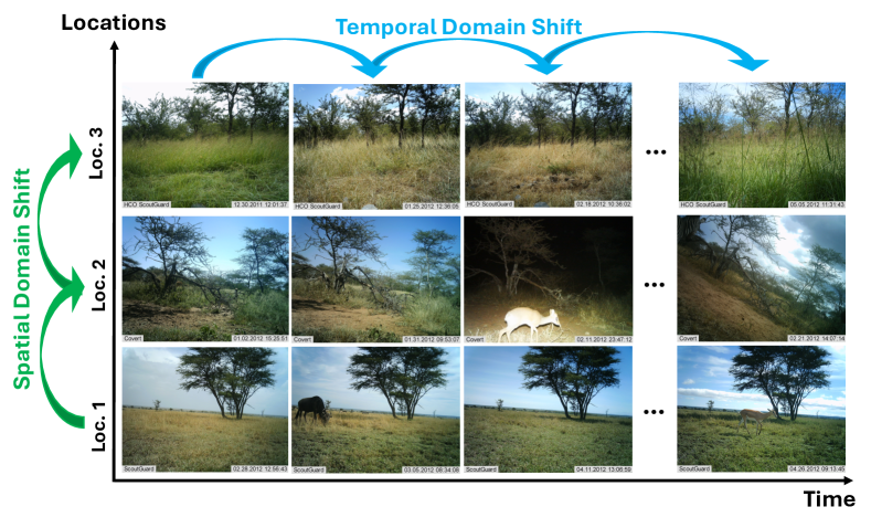
Figure 1. Spatial and temporal domain shifts in camera trap applications. In particular, Location 2’s camera position shifted over time while Location 1 and 3’s backgrounds show seasonal changes.

Locs.	Before	After	Acc.	Before	After	Acc.
	Spatial	Spatial	Drop	Temporal	Temporal	Drop
	Shift	Shift		Shift	Shift
1	78.8	66.4	12.4	80.6	52.1	28.5
2	78.8	19.3	59.5	67.9	59.2	8.7
3	78.8	66.3	12.5	87.9	63.8	24.1

Table 1. The wildlife classification model accuracy before and after spatial and temporal domain shifts on 3 test locations (R06, R09, and T11) of Serengeti S4 (Snapshot Serengeti, [n. d.])

The challenge of achieving robust domain generalization capability is compounded by the limited resources available on IoT devices. While a wide range of methods for domain generalization have proven effective (e.g. domain alignment (Muandet et al., 2013), meta-learning (Li et al., 2018), data augmentation (Volpi et al., 2018; Li et al., 2021), and ensemble learning (Arpit et al., 2022; Yeo et al., 2021)), the wide range of variations in data means that the model needs increased capacity (e.g., more layers, parameters) to learn and represent the broader set of features that distinguish one domain from another. This presents a significant challenge for enabling easy generalization on resource-constrained devices.

Performance degradation due to domain shifts. Table 1 shows the performance gap caused by spatial and temporal domain shifts when using EfficientNet-B0, a small classification model that is typically used on IoT platforms. To demonstrate the impact of spatial domain shifts, we trained a wildlife classification model using images from 154 camera trap locations in the Serengeti S4 dataset (details in §4.1). The ”Before Spatial Shift” accuracy is measured on samples from the same 154 locations, excluding those used in training. Testing the model on three new, unseen locations reveals that spatial domain shifts can cause accuracy drops of 12%–60%.

We use the same three locations to highlight the impact of temporal domain shifts. The data from each location is split into three equal chunks. The model is trained using data from the mentioned 154 locations, along with 20% of the beginning of the first chunk. ”Before Temporal Shift” accuracy is computed on the remaining 80% of the first chunk. To assess ”After Temporal Shift” accuracy, we test on the last chunk, which likely has the greatest temporal shift, resulting in a 9-28% performance drop.

We see that both these shifts can have substantial impact on performance. A model trained on data from one location may perform poorly when deployed in a different environment with unfamiliar backgrounds or lighting conditions. In addition, the specific species of animals that are frequent in an area can vary across locations and seasons, further complicating the classification task.

Our goal. In this paper, we aim to reconcile the conflicting goals of achieving high domain generalization performance and ensuring efficient inference for camera trap applications via continuous model fine-tuning. The basic idea is to deploy an ML model that is tailored to the current location and time window, allowing for both high efficiency and accuracy for the current domain. Whenever the domain shifts, the model can be fine-tuned to maintain robust classification accuracy on a new domain – that is, new animal images from different locations and time periods.

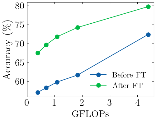
(a) A new location.

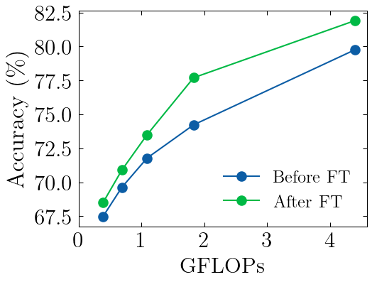
(b) A different time.

Figure 2. The trade-off between model complexity and generalization accuracy on images from a new location (a) and different time period (b). We evaluate five models, increasing in complexity from EfficientNet-B0 to B4, on location T08 of the Serengeti S4 dataset.

This approach is motivated by the observation that smaller models, when fine-tuned on the target domain, can achieve the accuracy of larger models. Figure 2 illustrates the trade-off between domain generalization performance, measured by classification accuracy on unseen images, and model complexity, measured by the number of floating-point operations (FLOPs), and the effectiveness of fine-tuning on the smaller models. We see that models from the EfficientNet family (Tan and Le, 2019), ranging from lightweight EfficientNet-B0 to complex EfficientNet-B4, have significant gaps in their generalization performance in images collected from a new location and at a different time. Larger models exhibit better domain generalization capability, while smaller models, though more efficient, perform worse on unseen data.

However, fine-tuning the smaller model can narrow the gap significantly. We can see that EfficientNet-B0, after fine-tuning using images from a new location, outperforms EfficientNet-B3 (before fine-tuning) while using significantly fewer FLOPs (6% accuracy gain but 4.7$\times$ fewer FLOPs) and is not far from EfficientNet-B4 (5% lower accuracy but 11.2$\times$ fewer FLOPs). Thus, our core argument is that instead of developing a single large model, we can use smaller, adaptable models that are both accurate and computationally efficient, meeting the resource constraints of camera traps while effectively handling domain shifts.

Research Challenges. The basic idea of continuous model fine-tuning presents several challenges. First of all, fine-tuning must be proactive. When temporal or spatial domain shifts occur, the model must be adapted to the new domain before a dataset of animal images from that domain is collected. This is crucial for maintaining high accuracy, as the model must be prepared to correctly classify incoming animal images. Existing domain adaptation approaches fall short in this context because they assume that target data, whether labeled or not, are available for model fine-tuning – an assumption that does not apply in our scenario.

In addition, fine-tuning must be both efficient so that it can be executed locally on an IoT device if needed and effective, achieving rapid updates with minimal time costs and high classification accuracy. In particular, the fine-tuning methods should be amenable to execution on-device since we cannot assume that camera trap nodes deployed in remote areas have good internet connectivity. Thus, we need methods that can adapt smaller, resource-efficient models to new environments without relying on extensive data transfer or manual annotation. Such in-situ fine-tuning allows the model to adapt to the new environment directly on the device, using only the data it can collect and process locally. This approach is crucial because we cannot fully observe or anticipate the characteristics of a new environment without actually deploying the camera trap.

WildFiT. To address these challenges, we identify and leverage domain-specific opportunities unique to camera trap applications. In these applications, the camera is typically static, resulting in relatively stable background scenes across images. While collecting images containing the target animals in a new domain is impractical—since the model needs to be adapted beforehand—background images without animals are easily obtainable from new locations or during different time periods.

To enable rapid, effective, and proactive fine-tuning, we propose a method called background-aware data synthesis. This technique generates training images that closely represent the new domain by blending these background images with animal images from the source domain. The synthesized images are then used to fine-tune the classification model. This approach allows for proactive fine-tuning by generating a diverse set of training images that reflect the target domain’s environmental conditions, without requiring actual animal images after a domain shift. Additionally, the synthesis pipeline is simple and efficient, making it suitable for real-time application alongside other data augmentation techniques during model fine-tuning. We refer to this process as background-aware fine-tuning.

To further enhance the effectiveness of fine-tuning, we introduce two additional optimizations. The first, background drift detection, continuously monitors the camera trap environment to collect representative background images for background-aware data synthesis. This method is based on the premise that not all background images contribute equally to fine-tuning performance; instead, using a set of recent and representative background images can help synthesize higher-quality datasets, thereby improving model accuracy. The second optimization, class distribution drift detection, utilizes recent animal class distributions detected by the on-device classification model to inform the background-aware data synthesis process. It aligns the distribution of synthesized animal images with the observed recent class distributions, further enhancing fine-tuning performance.

We conducted extensive evaluation of the performance of WildFiT across three camera trap datasets and two IoT processors. Our results show that:

• WildFiT’s background-aware data synthesis outperforms no fine-tuning by 23% in accuracy on average and outperforms other computationally efficient approaches (Yun et al., 2019; ZHANG, 2017) by 10.4%, all while being computationally more efficient (6.9ms vs 10-11ms on a CPU).

• Our method also achieves 1.7% higher accuracy on average compared to diffusion model-based synthesis approaches (Song et al., 2023; Zhang et al., 2023), while being three orders of magnitude faster (6.2 ms on CPU vs 6 — 13 seconds per image on NVIDIA RTX8000) and requiring no additional memory.

• End-to-end results show that WildFiT significantly outperforms several domain adaptation approaches such as using pseudo labels or even using ground-truth labels of animals in the new location to fine-tune.

• Our ablation study shows that the Background Drift Detection module improves accuracy by 2.4–6% for the different datasets compared to using only background-aware synthesis. The Class Distribution Drift Detection module further enhances performance, adding about 1–3.4% accuracy improvement.

• We show that running WildFiT fully (synthesis + standard augmentation + data loading) on a batch of 12 images takes about half to quarter of a second on Raspberry Pi 4 and 5. These show that WildFiT is highly practical for real-world use on IoT devices.

2. Background and Related Works

This section first introduces camera trap applications and then discusses related works and their limitations.

2.1. Camera Trap Applications

A camera trap is a camera that is automatically triggered by motion in its vicinity, like the presence of an animal or a human being. Camera trap applications play a critical role in wildlife monitoring, conservation, and ecological research by providing invaluable data on animal behavior, population dynamics, and biodiversity (Science, 2024). These automated systems capture vast amounts of image and video data from remote and often inaccessible locations, offering insights that would be impossible to obtain through manual observation.

ML in Camera Trap Applications. The sheer volume of data generated by camera traps presents a significant challenge for timely analysis and interpretation. This is where machine learning (ML) becomes indispensable. ML algorithms enable the efficient processing and classification of camera trap images, automating the identification of species, tracking of animal movements, and detection of rare or endangered species. These ML models can be deployed directly on camera trap devices, particularly when these devices are equipped with edge computing capabilities. This allows the camera traps to process data locally, rather than sending all the data to a central server for analysis. Deploying ML models on these devices reduces the need for constant data transmission, which is crucial for conserving battery life and managing limited bandwidth, especially in remote locations. Due to the constraints of IoT devices, such as limited computational power, memory, and energy, these ML models are often lightweight and optimized for efficiency. Techniques like model compression, pruning, and quantization are commonly used to make the models suitable for deployment on such resource-constrained devices (Rastikerdar et al., 2024).

The Generalization Problem. The generalization problem in camera trap applications is caused by domain shifts, which refer to the distribution shift between a set of training (source) data and a set of test (target) data. Domain shifts can cause a well-trained ML model to perform arbitrarily worse on the target data. Mathematically, let $\mathcal{X}$ be the input (feature) space and $\mathcal{Y}$ be the target (label) space. A domain is defined as a joint distribution $P(X,Y)$ on $\mathcal{X}\times\mathcal{Y}$. In the context of wildlife classification, $\mathcal{X}$ represents images containing animals of interest (also called animal images) while $\mathcal{Y}$ represents the set of animal labels or classes. We have training data $\mathcal{S}=\{(x,y)\}$ sampled from the source domain distribution $P^{\mathcal{S}}(X,Y)$. The goal of domain generalization is to learn a predictive model $f:\mathcal{X}\rightarrow\mathcal{Y}$ using source domain data $\mathcal{S}$ such that the prediction error on an unseen target domain data $\mathcal{T}=\{(x^{\mathcal{T}})\}$, sampled from the target domain distribution $P^{\mathcal{T}}(X,Y)$ ( $P^{\mathcal{T}}(X,Y)\neq P^{\mathcal{S}}(X,Y))$, is minimized.

2.2. Related Work and Limitations

While there is extensive literature on how to deal with domain shifts, we show that existing approaches cannot solve the generalization problem in camera trap applications due to various limitations.

Domain Adaptation. Domain adaptation (DA) focuses on adapting a model trained on the source domain to perform well on a different but related target domain. Typically, DA methods assume the availability of labeled or unlabeled target data for model adaptation, making them a poor fit for wildlife monitoring applications. For example, when cameras are deployed in new locations, it is impractical to collect images of animals from each new site in advance. The limitations of this approach are further highlighted in § 3.2 to motivate the importance of data synthesis.

Some DA approaches, known as zero-shot DA, attempt to generalize to unseen target domains by leveraging auxiliary information about the target domain even if they don’t have direct target domain data during training. For example, ZDDA (Peng et al., 2018) and CoCoGAN (Wang and Jiang, 2019) learn from the task-irrelevant dual-domain pairs, while Poda (Fahes et al., 2023) uses natural language descriptions of the target domain. These approaches cannot be applied, as they rely on auxiliary information that is unavailable for wildlife animal classification tasks.

Domain Generalization. Domain generalization (DG) aims to create models that are inherently robust to domain shifts by ensuring good performance across various source domains. Unlike DA, DG assumes no access to target domain data during training. DG methods can be categorized into domain alignment (Muandet et al., 2013), meta-learning (Li et al., 2018), ensemble learning (Zhou, 2012), and foundation models (Bommasani et al., 2021). However, achieving strong generalization often requires computationally complex models, as seen in recent foundation models (Bommasani et al., 2021), and are therefore not suitable for resource-constrained IoT devices.

Data Augmentation. Data augmentation approaches can generally improve the robustness of ML models. The existing literature roughly falls into the following groups: hand-engineered transformations (Shi et al., 2020), adversarial attacks (Volpi et al., 2018), learned augmentation models (Huang and Belongie, 2017; Choi et al., 2019), feature-level augmentation (ZHANG, 2017; Yun et al., 2019), and more recently generative models such as diffusion models (Trabucco et al., 2023).

The most relevant for us are feature-level augmentation techniques such as CutMix (Yun et al., 2019) and MixUp (ZHANG, 2017) that generate synthetic images by blending objects of interest with background images. Despite their efficiency, we show that these generic techniques do not produce high-quality synthetic animal images, resulting in limited, if any, performance improvement. This is because these methods often strive to augment images in a domain-agnostic way, which can improve model robustness but may not capture the specific characteristics of new deployment environments.

Diffusion models, on the other hand, offer the potential for high quality, realistic, image synthesis that can better match target scenes. Off-the-shelf diffusion models can be leveraged to generate synthetic target domain animal images by combining a source domain animal image with a target domain background (Zhang et al., 2023; Song et al., 2023; Niu et al., 2021). However, these incur immense computational cost making them infeasible for rapid, in-situ adaptation to changing scenes, even with cloud resources. In addition, fine-tuning these models to specific wildlife applications would require substantial datasets and fine-tuning, which is often not feasible in practice.

Drift Detection. While the previous approaches focus on adapting to or generalizing across domains, WildFiT goes a step further by incorporating drift detection techniques to continuously optimize its adaptation process. Drift detection in ML traditionally focuses on identifying changes in data distribution that can impact model performance over time. The literature includes various approaches, such as statistical hypothesis testing, distance-based metrics, and ensemble methods (Van Looveren et al., 2019; Lipton et al., 2018). WildFiT leverages statistical methods such as Least-Squares Density Difference (LSDD), which are frequently employed to detect shifts in data streams (Rabanser et al., 2019). These methods are chosen for their computational efficiency, making them suitable for execution on IoT devices.

3. Design of WildFiT

WildFiT is a wildlife classification system designed to achieve both high domain generalization performance in recognizing animals of interest and high efficiency in on-device inference. It bridges the gap between various techniques discussed in § 2.2, combining strengths from multiple areas while overcoming their individual limitations:

• Adaptability without target data: Unlike traditional DA methods, WildFiT adapts to new environments without requiring labeled or unlabeled target data. It differs from zero-shot DA in its use of easily obtainable background images as auxiliary information and its ability to continuously adapt in-situ.

• Generalization with efficiency: Unlike existing domain generalization (DG) approaches, WildFiT leverages domain-specific information (background images) to perform proactive model fine-tuning, enabling the use of smaller and more efficient models while maintaining strong performance across domain shifts.

• Targeted augmentation: Unlike generic augmentation methods, WildFiT performs domain-specific data synthesis using background images from the new deployment location. This targeted approach, combined with computationally efficient synthesis techniques, improves data quality and allows rapid and effective adaptation to domain shifts without significant computational resources.

• Continuous adaptation: Through drift detection, WildFiT dynamically adjusts to gradual or abrupt changes in environments. This distinguishes WildFiT from traditional DA methods, which often assume a static target domain. By continuously adapting to changing conditions, WildFiT enhances long-term effectiveness in wildlife monitoring applications.

This combination of features allows WildFiT to address the specific challenges of wildlife monitoring applications more comprehensively than existing approaches. We next provide an overview of WildFiT and then detail the key system components that address the challenges of continuous model fine-tuning.

3.1. Overview of WildFiT

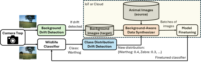
Figure 3. Overview of WildFiT for cloud-assisted and local-only (unattended) scenarios. In case the communication or the cloud is not available, the system relies on on-device fine-tuning to adapt to domain shifts. The yellow-colored components sit on the device, together with the rest of the components. In cloud-assisted mode, the yellow-colored components can be offloaded to the cloud.

Figure 3 illustrates the design of WildFiT. WildFiT runs a wildlife classification model on an IoT device to identify animals of interest captured by a motion-triggered camera. Concurrent to the inference on every incoming frame, WildFiT includes three main components to enable rapid, effective, and proactive model fine-tuning.

The first component, the Background-Aware Data Synthesizer (“Synthesizer” for short), creates training images that mimic the target domain by integrating objects (e.g., animals of interest) from the source domain into background images captured in the target environment. The synthesized data are used to adapt the wildlife classifier to the target domain.

The second component, the Background Drift Detector (BDD), identifies changes in background images that suggest a shift in the environmental setting. By detecting these drifts, the system can update the background images used in the synthesizer, enabling the fine-tuning of the IoT model before animals in these new environments occur.

The third component, the Class Distribution Drift Detector (CDD), monitors the class distribution based on the IoT model’s predictions on recent frames. This allows the system to fine-tune the model whenever a drift in class distribution is detected. WildFiT then adjusts the distribution of synthesized images from the Synthesizer to match the recent class distribution and updates the model accordingly.

Usage Scenarios. WildFiT operates in both cloud-assisted and unattended modes. When cloud assistance is available, the Synthesizer and model finetuning run on the cloud. The cloud maintains a repository of background images and the class distribution, initialized when a camera trap is installed at a new location and updated over time. If the BDD executed on the device identifies a new background image indicating an environmental shift, the image is sent to the cloud to update the repository. Similarly, when the CDD on the device detects a change in class distribution, the new distribution is sent to the cloud for repository updates and triggers a model fine-tuning. WildFiT fine-tunes the model in the cloud using a mix of synthesized images, background images from the target domain, and training images from the source domain, and then updates the on-device model accordingly.

For unattended operations, where cloud availability is not an option, WildFiT relies on local model fine-tuning. To support local fine-tuning, the IoT device stores training images from the source domain as well as animals of interest for data synthesis. In § 4.5, we demonstrate that such on-device storage requirement is feasible on the evaluated IoT platforms. We next describe the three key components of WildFiT in more detail.

3.2. Background-Aware Data Synthesizer

The Synthesizer tackles a crucial challenge for WildFiT: the lack of high quality training samples (i.e., animal images) from the target domain, which are essential for adapting the on-device classification model after a domain shift. This section first highlights the importance of data synthesis in overcoming the challenge and then elaborates on the proposed synthesis pipeline.

The Importance of Data Synthesis. Since fine-tuning requires target domain data, we explain why traditional domain adaptation methods, which rely on collecting data from the target domain, are not an ideal solution. Domain adaptation approaches react to domain shifts by retraining the model with a mix of target domain data and source domain data. This involves waiting for animals to appear after a domain change and manually generating their ground truth labels or generating their pseudolabels using the wildlife classification model trained on the source domain data. These labels or pseudolabels are then used to fine-tune the model and adapt to the changing environment. Although this approach is computationally efficient, it suffers from two major drawbacks, as we show empirically in Section 4.5. First, due to the poor performance of the classification model after domain shifts, pseudolabels can be highly noisy, resulting in limited performance improvement from fine-tuning. Second, since animals appear relatively infrequently, there can be a significant delay in collecting enough animal images from the target domain. Concurrently, the background continues to change, so adaptation is ineffective and fine-tuning is constantly catching up to the current environment. Due to the lack of sufficient target domain data before the domain shifts again, the performance is still sub-optimal even when ground truth labels are available.

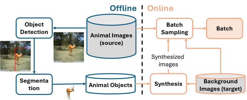
Figure 4. The background-aware synthesis pipeline.

The Proposed Synthesizer. Our proposed Synthesizer addresses these challenges by eliminating the need for target domain data. It leverages the insight that background images from the target domain are readily available in camera trap applications and can be used to generate synthetic animal images that closely align with the target domain’s data distribution. Figure 4 illustrates the synthesis pipeline, which consists of an offline phase executed once and an online phase executed during model fine-tuning to create synthetic images on-the-fly.

The offline phase: This phase creates a repository of animal objects by extracting them from the training images. We utilize MegaDetector V5 (Morris, [n. d.]) to identify the bounding box around each object, then pass the image and the bounding box information to the Segment Anything model (Kirillov et al., 2023) to extract the object’s mask and isolate the object image.

The online phase: The online phase samples animal objects and blends them with background images to synthesize animal images. This involves overlaying the object onto a random background image from the target domain. While the placement of the object could be random, our observations indicate that placing the object in a location corresponding to its original position yields higher accuracy. Therefore, we use the bounding box data from MegaDetector V5 to accurately position the object within the background. Additionally, we synthesize images containing multiple animals (herds) to effectively represent similar scenarios in the target domain.

3.3. Background Drift Detector

WildFiT needs to adapt the model to temporal domain shifts. However, transmitting or storing all background images is impractical due to communication limitations in cloud-assisted scenarios and storage constraints on IoT devices in local-only scenarios. Therefore, it is essential to detect background images that indicate significant temporal shifts and provide valuable new information. This requires knowing when to transmit (in cloud-assisted scenarios) or store (in local-only scenarios) a background image.

To address this challenge, we developed the Background Drift Detector (BDD), which evaluates whether the current background image significantly differs from those recently collected and, if so, updates the background image repository. Unlike traditional drift detection methods discussed in § 2.2, our detector specifically targets shifts in background images rather than animal images. Reliable drift detection in images remains an unsolved problem due to the high dimensionality of images, often requiring computationally intensive dimension reduction techniques to identify appropriate representations for hypothesis testing (Rabanser et al., 2019), making them unsuitable for IoT devices. Our drift detector BDD, however, leverages domain-specific knowledge to achieve both high efficiency and effectiveness.

BDD operates on IoT devices and works as follows. It maintains the last $N$ collected backgrounds ($bg_{pool}$) on the device to compare against the current background ($bg_{cur}$). Initially, from the pool ($bg_{pool}$), it identifies backgrounds collected within one hour before or after the times of the current background ($bg_{cur\pm 1hr}$). From this subset, the background with the closest date to $bg_{cur}$ is selected. If multiple candidates remain, the one with the closest time to $bg_{cur}$ is chosen as $bg_{ref}$. Finally, both $bg_{cur}$ and $bg_{ref}$ are analyzed using the Least-Squares Density Difference (LSDD) method (Bu et al., 2018; Van Looveren et al., 2019), which compares their pixel-level distributions. A drift is determined based on a p-test with a 5% significance level. Detected images are incorporated into the previously collected background images and consumed by the Synthesizer.

3.4. Class Distribution Drift Detector

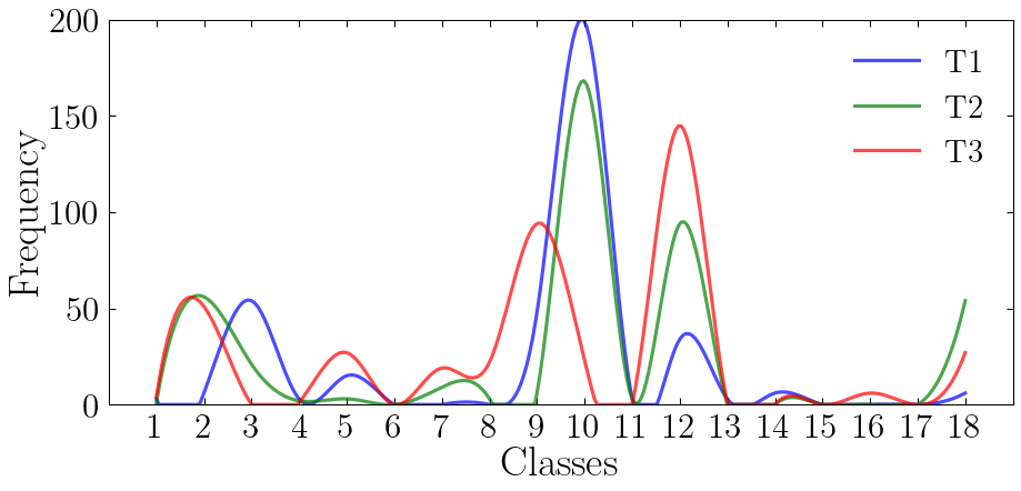
Figure 5. Class distribution changes across time (location U10 from Serengeti S4 dataset)

To further optimize the adaptation process in WildFiT, we introduce a module called the Class Distribution Drift Detector (CDD), which tracks the distribution of predictions on the IoT device and detects when a drift in class distributions occurs. This module is motivated by the observation that the animal class distribution changes across locations and across time. By continuously aligning the synthesized image distribution to the target domain distribution, CDD is expected to further boost finetuning performance.

Figure 5 shows the class distribution of a test location in the Serengeti S4 dataset (Snapshot Serengeti, [n. d.]) across three consecutive time windows. The distribution exhibits drift over time. Specifically, comparing the T1 curve with T2 and T3 reveals increasing divergence as time progresses, with T3 showing a pronounced drift and T2 exhibiting a lighter shift.

CDD operates on IoT devices and works as follows. We use the Chi-Squared statistical test for drift detection, as it is well-suited for categorical data. Once at least $C$ samples are collected, the recent class distribution and the class distribution from the previous fine-tuning cycle are input into the Chi-Squared drift detector. Using a p-test with a 5% significance level, it determines whether a drift has occurred. If a drift is detected, we fine-tune the IoT model based on the new class distribution.

4. Evaluation

We first describe the experiment settings in §4.1, and then evaluate the three key system components Background-Aware Data Synthesizer, Background Drift Detector (BDD), and Class Distribution Drift Detector (CDD) in §4.2-4.4. We further perform end-to-end evaluations of WildFiT in §4.5, and ablation studies in §4.7.

4.1. Experiment Settings

Datasets. We utilize three datasets as shown in Table 2: two from the Serengeti Safari Camera Trap network (referred to as D1 and D2) (Snapshot Serengeti, [n. d.]), and one from the Enonkishu Camera Trap dataset (referred to as D3) (Snapshot Enonkishu, [n. d.]). These datasets are chosen since they have temporal data over relatively long durations and across several locations captured by trail cameras, hence they exhibit real-world temporal and spatial domain drifts. The Camera Trap datasets normally include a lot of species plus an empty class whose images show a scene with no species in it. Some species lack enough samples for both training and testing sets. Therefore, we selected the 18 most frequent species from the Serengeti dataset and 10 from the Enonkishu dataset for classification. Including the empty class, this results in 19 classes for Serengeti and 11 for Enonkishu. Table 2 lists the data statistics. “Train” are the locations whose animal images are used to train the classification model while “Test” refers to those used to evaluate spatial domain shifts.

	Train		Test
Dataset	# Locations	# Images	# Locations	# Images
Serengeti S1 (D1)	153	3692	15	48063
Serengeti S4 (D2)	154	6650	27	82263
Enonkishu (D3)	11	1043	5	11003

Table 2. Summary of training and test data statistics across different datasets.

Implementation of WildFiT. The wildlife classifier is trained in PyTorch using a two-stage pipeline on the source domain data to ensure high model quality. It employs the EfficientNet-B0 model pre-trained on ImageNet (Deng et al., 2009). In the first stage, the classification head is trained for 5 epochs with a learning rate (lr) of 1e-3 while keeping the backbone frozen. In the second stage, the entire network is trained for 30 epochs with an lr of 1e-5, using an early stopping criterion of 2 epochs. For fine-tuning over time (BDD and ADD), we maintain the same lr of 1e-5. The Adam optimizer (Kingma, 2014) is used along with a cross-entropy loss function.

The background repository is initialized with $40$ images and expands as BDD detects new samples. The last 20 background images are stored on the device for drift detection. The wildlife classifier is fine-tuned weekly by default, using a combination of source domain images and those synthesized with the latest background repository. If the latest class distribution contains at least $C=100$ predictions, it is used for fine-tuning; otherwise, the previous distribution is applied.

Additional model finetuning can be triggered by the CDD module. When $C=100$ new predictions are collected, the class distribution of these predictions is compared to the previous one using a Chi-Squared test. If drift is detected, the model is fine-tuned with the new class distribution. After fine-tuning, the process restarts by collecting another $C=100$ predictions for the next CDD cycle.

We profiled the latency of WildFiT’s synthesis pipeline and EfficientNet-B0 fine-tuning on Raspberry Pi 4B and Pi 5. A cluster of NVIDIA RTX8000 48GB GPUs was used for model training.

4.2. Eval. of Background-Aware Synthesis

Baselines. We compare our approach against three classes of techniques that offer different compute-accuracy tradeoffs:

(1) No fine-tuning (No-FT), which serves as a lower bound baseline. Our goal is to significantly outperform this approach, demonstrating the clear benefits of our method.

(2) Computationally efficient approaches, which are efficient enough to feasibly execute on-device on IoT hardware. These include: (a) CutMix (Yun et al., 2019) (CUT), a data augmentation technique that combines two images by cutting and pasting patches and mixing their labels proportionally. We adapted CutMix to synthesize images by pairing a source image with a background image from the target domain. (b) MixUp (ZHANG, 2017) (MIX), a data augmentation technique that creates new training samples by linearly blending pairs of images and their labels. Similar to CutMix, we adapted MixUp to blend source images with target backgrounds. These approaches are in the same computational ballpark as our techniques. Our objective is to outperform these methods while having similar or better computational efficiency.

(3) Diffusion model-based approaches, which are currently infeasible to execute on-device and may even be too slow or expensive to run repeatedly in a cloud environment. These include: (a) Object-Stitch (Obj-St) (Song et al., 2023), an object compositing method based on conditional diffusion models, specifically designed for blending objects into background images. (b) ControlCom (CC) (Zhang et al., 2023), a method that synthesizes realistic composite images from foreground and background elements using a diffusion model. For these approaches, we focus on achieving similar accuracy while offering significant benefits in terms of on-device capability, cost-effectiveness, and continuous adaptability to changing domains.

For this evaluation, we first randomly selected 250 background images from each test location within the target domain and excluded them from the test set for each location. The selected backgrounds are used to synthesize animal images, which are then mixed with the training data and background images in each batch to fine-tune the classification model. The fine-tuned models are evaluated on images from the target domain using the D2 dataset.

Results on Classification Accuracy. Table 3 shows exhaustive results comparing our synthesis method against baselines across 27 test locations in D2 dataset. We see that: (1) compared to no fine-tuning, our synthesis scheme has a massive gain of 23% in accuracy on average (last row), (2) compared to computationally efficient approaches like CutMix (Yun et al., 2019) and MixUp (ZHANG, 2017), our method has a significant advantage of 10.4% on average, with 20-41% improvements in some locations where the spatial domain shift is large, and (3) compared to diffusion model-based approaches, our method generally performs better with 1.7% average gain (and in some locations more than 10%).

	Methods
Locs.	Ours	No FT	$\Delta 1$	Mix	Cut	$\Delta 2$	Obj-St	CC	$\Delta 3$
1	92.5	86.3	+6.2	84.2	86.9	+5.6	91.0	91.5	+1.0
2	93.3	85.8	+7.5	79.2	90.8	+2.5	90.8	91.7	+1.6
3	76.0	67.4	+8.6	35.7	49.9	+26.1	66.7	68.3	+7.7
4	92.7	80.2	+12.5	85.6	85.9	+6.8	88.9	90.2	+2.5
5	98.0	50.1	+47.9	97.5	97.5	+0.5	97.7	97.8	+0.2
6	93.0	19.3	+73.7	91.4	91.6	+1.4	92.1	92.1	+0.9
7	95.2	60.0	+35.2	91.8	92.8	+2.4	94.8	95.3	-0.1
8	93.4	43.9	+49.5	91.9	92.3	+1.1	94.1	94.6	-1.2
9	95.2	90.0	+5.2	94.2	94.6	+0.6	95.3	95.5	-0.3
10	85.1	78.4	+6.7	71.9	75.8	+9.3	87.0	87.5	-2.4
11	93.7	89.3	+4.4	86.8	89.4	+4.3	92.3	93.0	+0.7
12	89.7	92.2	-2.5	77.5	77.5	+12.2	88.8	90.0	-0.3
13	83.1	52.9	+30.2	81.5	83.2	-0.1	81.1	84.0	-0.9
14	90.0	33.9	+56.1	86.2	86.1	+3.8	89.2	90.1	-0.1
15	91.6	76.4	+15.2	83.5	87.4	+4.2	91.0	90.3	+0.6
16	83.7	61.9	+21.8	25.6	42.0	+41.7	64.3	70.4	+13.3
17	77.0	60.9	+16.1	51.1	54.3	+22.7	63.1	71.0	+6.0
18	82.6	56.3	+26.3	35.5	65.6	+17.0	73.9	78.7	+3.9
19	84.5	71.4	+13.1	51.3	62.1	+22.4	79.3	82.2	+2.3
20	74.9	66.4	+8.5	55.5	51.8	+19.4	72.5	75.7	-0.8
21	82.9	79.7	+3.2	67.3	73.1	+9.8	79.8	82.1	+0.8
22	89.5	50.3	+39.2	88.9	85.0	+0.6	90.4	91.8	-2.3
23	86.1	82.9	+3.2	66.3	72.6	+13.5	83.5	86.7	-0.6
24	83.6	66.7	+16.9	43.0	56.2	+27.4	66.0	73.5	+10.1
25	98.8	3.8	+95.0	98.2	98.4	+0.4	98.6	98.7	+0.1
26	86.3	79.2	+7.1	70.7	72.4	+13.9	83.2	84.0	+2.3
27	89.7	76.4	+13.3	76.5	79.4	+10.3	87.7	87.3	+2.0
All	88.2	65.2	+23.0	72.9	77.6	+10.4	84.6	86.4	+1.7

Table 3. Classification accuracy of our synthesis approach compared to baselines across 27 test locations in the D2 dataset. $\Delta 1$ represents the accuracy gain over no fine-tuning (No FT), $\Delta 2$ is the gain over the best resource-efficient alternative (MixUp or CutMix), and $\Delta 3$ is the gain over the best diffusion-based model (Object-Stitch or ControlCom). The last row shows the average across all locations.

Figure 6 presents example images synthesized by WildFiT and the alternatives. WildFiT produces images with similar visual quality to diffusion-based approaches but is much more computationally efficient, reflecting the comparable fine-tuning performance in Table 3. Notably, diffusion methods like ControlCom introduce artifacts (second and third rows), and Object-Stitch alters both the background and object, resulting in low fidelity in the third row.

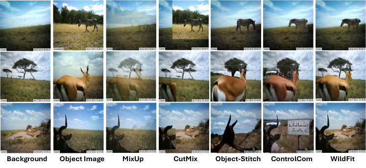
Figure 6. synthesized images from our approach and baselines.

Results on Synthesis Speed. Table 4 lists the time spent on synthesizing an image on an NVIDIA RTX8000 using different methods. We see that WildFiT has the lowest latency of 6.2ms per image, which is 40-50% lower latency for synthesis compared to other computationally lightweight methods MixUp and CutMix. Against diffusion model-based approaches Object-Stitch and ControlCom, WildFiT incurs three orders of magnitude less latency (6ms versus 6 — 13 seconds) while WildFiT synthesis does not require a GPU.

Methods	Latency	Device	Model Size
Mixup (ZHANG, 2017)	10.5 ms	CPU	$\mathrel{-}$
CutMix (Yun et al., 2019)	11.5 ms	CPU	$\mathrel{-}$
Object-Stitch (Obj-St) (Song et al., 2023)	6512 ms	GPU	4.9 GB
ControlCom (CC) (Zhang et al., 2023)	13198 ms	GPU	5.1 GB
WildFiT	6.2 ms	CPU	$\mathrel{-}$

Table 4. Computational efficiency for synthesizing a single image. We used NVIDIA RTX8000 for profiling both diffusion models.

4.3. Eval. of Background Drift Detection

The Background Drift Detector (BDD) module is designed to select representative background images for data synthesis. To assess its effectiveness. We compare our method against a periodic sampling approach, which selects background images at fixed intervals for model fine-tuning. The intervals tested are 4, 5, and 6 hours, meaning a minimum of 4, 5, or 6 hours must elapse between samples. We chose these numbers because they are close to the average sampling frequency of BDD, which is roughly one frame per 6 hours. We assess model accuracy by fine-tuning the classification model using synthesized images generated from the selected backgrounds. Both the BDD and baseline use the same fine-tuning procedure: the model is fine-tuned once per week, ensuring at least one week between fine-tuning cycles.

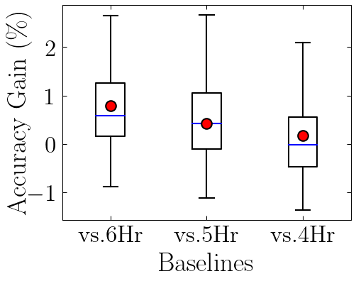
Figure 7. Accuracy gain of our method over periodic sampling baselines. Each box plot presents results aggregated across 27 test locations of the D2 dataset and the red dot shows the mean.

Figure 7 shows the accuracy gains over these sampling approaches. Overall, BDD has an accuracy gain of about 0.8% compared to regularly sampling at this frequency without being adaptive. Regularly sampling at higher frequencies bridges the gap with our method but results in more background sampling. BDD performs comparably to the approach that transmits every 4 hours, while samples 30% less.

4.4. Eval of Class Distr. Drift Detection

Class distribution drift detection monitors the distribution of animal classes and triggers model fine-tuning whenever a significant shift is detected. To assess the effectiveness of this module, we compare it against two baselines: (1) Init i.e. one-time fine-tuning of the model using the initial distribution of source domain data, followed by no subsequent fine-tuning over time, and (2) N-Week i.e. fine-tuning periodically at intervals of N weeks. We assessed this baseline with $N\in\{1,2,3\}$ weeks. For both our method and the baselines, we synthesize images using a sample of 250 background images. We measure the classification accuracy of the fine-tuned model aggregated on the 27 test locations of D2.

Figure 8 presents the finetuning frequency and accuracy gain of our approach (CDD) over various baselines, aggregated over 27 test locations from the D2 dataset. Compared to the Init baseline, CDD shows a mean accuracy improvement of approximately 2%, highlighting the effectiveness of our fine-tuning process. When compared to periodic fine-tuning schemes, CDD maintains competitive accuracy while reducing fine-tuning frequency. Specifically, CDD achieves mean accuracy improvements of 0.7%, 0.5%, and 0.2% over the 3-week, 2-week, and 1-week schemes, respectively. Importantly, CDD triggers fine-tuning on average 2.2 times, compared to 5.1, 2.4, and 1.7 times for the 1-week, 2-week, and 3-week schemes. This puts CDD on par with the 2-week scheme in terms of fine-tuning frequency, while still outperforming it in accuracy.

We note that minimizing fine-tuning frequency is crucial, as it introduces latency overhead in both cloud-assisted and local-only scenarios. In cloud-assisted settings, the IoT device must download the updated model, while local-only scenarios face significant computation overhead due to fine-tuning. Thus, our approach demonstrates a clear improvement in overall accuracy compared to periodic fine-tuning (N-Week), while maintaining a low fine-tuning frequency.

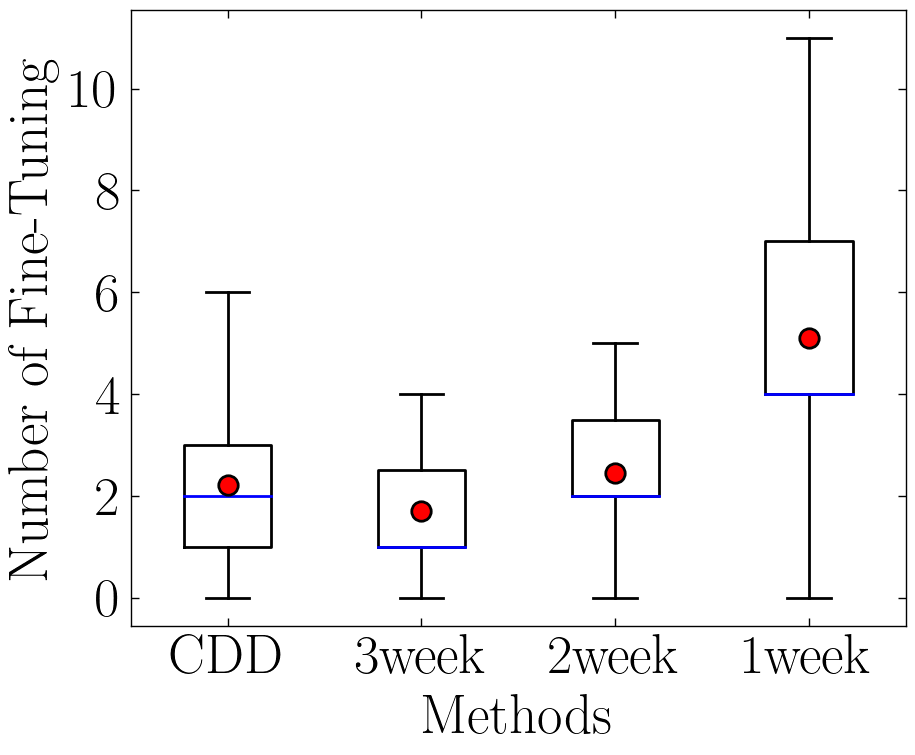
(a) Number of fine-tuning

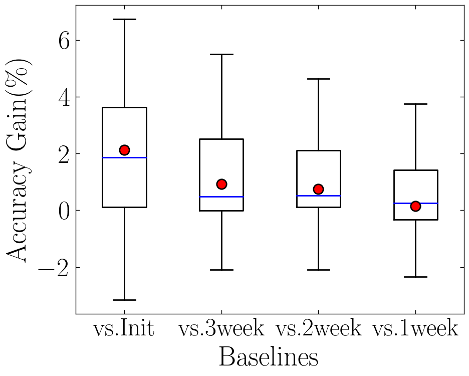
(b) Accuracy gain

Figure 8. (a) Number of Fine-tuning for different approaches and (b) accuracy gain for the model fine-tuned using our approach (i.e., fine-tuning whenever class distribution drift is detected) over baseline methods (i.e., no fine-tuning or periodic fine-tuning).

4.5. End-to-End Performance

This section reports the end-to-end evaluation of WildFiT’s performance in terms of model accuracy. The results apply to both the cloud-assisted and local-only scenarios. We compare the following approaches:

• Pseudolabel: This baseline assumes a few target domain animal images are collected for model fine-tuning. As ground truth labels are unavailable, it uses the IoT model (EfficientNet-B0 or B4), trained on the source domain, to generate pseudo-labels for fine-tuning.

• GTlabel: This approach assumes the target domain animal images have ground truth labels. While impractical, it gives us an upper-bound for the Pseudolabel method.

• WildFiT:Syn: This approach removes the Background Drift Detection (BDD) and the Class Distribution Drift Detection (CDD) modules from WildFiT to evaluate their importance. We start by initializing our background repository with the first 40 samples and perform a single round of model fine-tuning.

• WildFiT:Syn+BDD: This approach removes only the CDD module. Like WildFiT-Syn, the background repository is initialized with 40 images, but new backgrounds are added when BDD is triggered. Fine-tuning occurs at intervals of at least one week, meaning there must be at least one-week gap between fine-tuning sessions.

• WildFiT:All: This is the complete WildFiT system as shown in Figure 3.

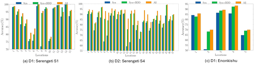
Figure 9. End-to-End performance of WildFiT with Synthesis alone, Synthesis + BDD, and Synthesis+BDD+CDD.

	Datasets
Methods	D1	D2	D3
Pseudolabel (B0)	56.1 (55.7)	64.4 (70.9)	64.2 (84.2)
Pseudolabel (B4)	58.3 (73.1)	67.0 (72.0)	66.7 (86.0)
GTlabel (B0)	82.2 (83.0)	80.8 (83.0)	78.6 (82.9)
GTlabel (B4)	82.0 (84.2)	84.3 (85.0)	81.3 (86.2)
WildFiT-Syn (B0)	89.1 (92.1)	80.3 (82.7)	74.3 (84.1)
WildFiT-Syn+BDD (B0)	92.5 (95.5)	86.9 (88.6)	80.1 (82.7)
WildFiT-All (B0)	93.5 (96.2)	90.3 (92.8)	81.9 (85.7)

Table 5. Mean and median (in parentheses) accuracies across test locations for end-to-end approaches.

For fair comparison, the number of sampled animal images in the Pseudolabel and GTlabel approaches is matched to the number of sampled background images using BDD in WildFiT, and the fine-tuning process is the same as WildFiT.

The results in Table 5 reveal several important insights about the performance of different approaches.

Comparison against pesudolabels. Firstly, the Pseudolabel approach performs poorly across all datasets, regardless of the model size. For instance, even with the larger EfficientNet-B4, the accuracy only reaches 58.3%, 67.0%, and 66.7% for D1, D2, and D3 respectively. This under-performance is primarily due to the inaccuracy of the pseudo-labels, highlighting the importance of proactive fine-tuning rather than relying on reactive approaches.

Comparison against ground truth labels. Even with ground truth labels, as in the GTlabel approach, performance remains suboptimal due to the infrequent and inconsistent appearance of animals. Different species appear at varying times, making it difficult to gather enough labeled data for effective fine-tuning. Additionally, by the time enough data is collected, temporal shifts may occur, further complicating adaptation. This is reflected in the GTlabel results, where even with EfficientNet-B4, accuracy reaches only 82.0%, 84.3%, and 81.3% for D1, D2, and D3, respectively.

Compared to both the above methods, WildFiT (last row) is significantly better with average accuracies of 93.5%, 90.3% and 81.9% for D1, D2 and D3 respectively.

4.6. Local-Only WildFiT

We now consider the performance of WildFiT in the case of unattended operation where fine-tuning occurs entirely at the IoT device deployed on-site without needing to communicate with the cloud. This is important in practice for Camera Trap deployments in remote locations where nodes often need to rely on solar power and have weak cellular connectivity.

Operation (batch=12)	RPi-4B	RPi-5
DataLoader (4 workers)	137 ms	106 ms
Standard Aug + DataLoader	386 ms	257 ms
- RandomFlip	7 ms	3 ms
- Rotation	14 ms	8 ms
- ColorJitter	170 ms	95 ms
- Normalization	58 ms	46 ms
WildFiT: Syn + StdAug + DL	417 ms	270 ms
Fine-tuning EfficientNetB0 (per iter)	66.78 s	36.12 s

Table 6. Performance comparison of synthesis and training operations on Raspberry Pi 4B (8GB) and Pi5 (8GB). DL refers to DataLoader.

We see from Table 6 that WildFiT is extremely efficient in generating synthetic images. For example, on the Raspberry Pi 5, WildFiT adds only 13ms to standard augmentation and data loading. The total time for synthesizing, applying standard augmentations, and loading a batch of 12 images is only 270 ms on the Raspberry Pi 5, which is significantly faster than the 36.12 seconds required for training a single batch with EfficientNetB0. This speed difference allows for the generation of a large number of synthetic images during the time it takes to train on a single batch, greatly enhancing the diversity and quantity of training data available. The results show that WildFiT has very low computational overhead and is highly practical for real-world use on resource-constrained platforms, while allowing our wildlife classification system to continuously adapt to changing environments.

The local-only setting requires approximately 1.8GB for storing 350 samples per class and 600MB for storing 100 samples per class (including both the original training set and extracted objects). Since devices like Raspberry Pi 4B and Pi5 have up to 8GB RAM and support up to 32GB SD cards, they can easily accommodate the necessary data for local-only operations.

4.7. Ablation Studies

Breakdown per module. The last three rows of Table 5 demonstrate that each stage of WildFiT contributes to performance improvement. The background-aware synthesis approach (Syn) alone is similar in performance to GTlabel (B0) and achieves 89.1%, 80.3%, and 74.3% accuracy for D1, D2, and D3 respectively. Adding Background Drift Detection (BDD) results in significant gains, improving accuracy by 2.4% for D1 and approximately 6% for both D2 and D3. The inclusion of Class Distribution Drift Detection (CDD), completing our full WildFiT approach, further enhances performance. It adds about 1-1.8% accuracy improvement for D1 and D3, and a more substantial 3.4% for D2.

Figure 9 provides an exhaustive breakdown of the performance of each stage of WildFiT on each location of the three datasets - D1, D2 and D3. We clearly see the diversity in the gains provided by each technique — the benefits of the synthesis method dominates in several locations but there are many locations where nearly all gains come from BDD or CDD. These results show that each component of our method provides benefits, with their impact varying across different datasets and locations depending on the types of shifts seen in these deployments.

	Training Size (Per Class)
Methods	100/class	350/class	700/class
No-FT	53.1	65.2	67.1
WildFiT	85.5	88.2	90.0
Accuracy gain	+32.4	+23.0	+22.9

Table 7. Effect of number of training samples (averaged over 27 test locations of D2 dataset).

Number of Training Data (Tr). Table 7 shows the effect of the number of training data instances per class on the performance of WildFiT vs no fine-tuning. The evaluation setting is the same as § 4.2. We see that WildFiT scales down very well — even when the number of training instances drops from 700 to 100, the loss in accuracy is only 5% whereas no fine-tuning drops by 15%.

5. Conclusions

This work introduces WildFiT, a novel approach to reconcile the conflicting goals of achieving high domain generalization performance and ensuring efficient inference for camera trap applications. By leveraging continuous model fine-tuning and background-aware data synthesis, we demonstrate that smaller, adaptable models can match the accuracy of larger models while maintaining computational efficiency on resource-constrained IoT devices. The effectiveness of WildFiT in handling both spatial and temporal domain shifts opens up new possibilities for wildlife monitoring in diverse and changing environments. While we focused on wildlife classification in this work, the principles of continuous adaptation and efficient on-device fine-tuning may have broader applicability in other IoT domains where environmental conditions are dynamic and impact how we approach model deployment in resource-constrained, real-world settings.

References

- (1)
- Arpit et al. (2022) Devansh Arpit, Huan Wang, Yingbo Zhou, and Caiming Xiong. 2022. Ensemble of averages: Improving model selection and boosting performance in domain generalization. Advances in Neural Information Processing Systems 35 (2022), 8265–8277.
- Beery et al. (2018) Sara Beery, Grant Van Horn, and Pietro Perona. 2018. Recognition in terra incognita. In Proceedings of the European conference on computer vision (ECCV). 456–473.
- Blanchard et al. (2011) Gilles Blanchard, Gyemin Lee, and Clayton Scott. 2011. Generalizing from several related classification tasks to a new unlabeled sample. Advances in neural information processing systems 24 (2011).
- Bommasani et al. (2021) Rishi Bommasani, Drew A Hudson, Ehsan Adeli, Russ Altman, Simran Arora, Sydney von Arx, Michael S Bernstein, Jeannette Bohg, Antoine Bosselut, Emma Brunskill, et al. 2021. On the opportunities and risks of foundation models. arXiv preprint arXiv:2108.07258 (2021).
- Bu et al. (2018) Li Bu, Cesare Alippi, and Dongbin Zhao. 2018. A pdf-Free Change Detection Test Based on Density Difference Estimation. IEEE Transactions on Neural Networks and Learning Systems 29, 2 (2018), 324–334. https://doi.org/10.1109/TNNLS.2016.2619909
- Choi et al. (2019) Jaehoon Choi, Taekyung Kim, and Changick Kim. 2019. Self-ensembling with gan-based data augmentation for domain adaptation in semantic segmentation. In Proceedings of the IEEE/CVF international conference on computer vision. 6830–6840.
- Deng et al. (2009) Jia Deng, Wei Dong, Richard Socher, Li-Jia Li, Kai Li, and Li Fei-Fei. 2009. Imagenet: A large-scale hierarchical image database. In 2009 IEEE conference on computer vision and pattern recognition. Ieee, 248–255.
- Fahes et al. (2023) Mohammad Fahes, Tuan-Hung Vu, Andrei Bursuc, Patrick Pérez, and Raoul De Charette. 2023. Poda: Prompt-driven zero-shot domain adaptation. In Proceedings of the IEEE/CVF International Conference on Computer Vision. 18623–18633.
- Huang and Belongie (2017) Xun Huang and Serge Belongie. 2017. Arbitrary style transfer in real-time with adaptive instance normalization. In Proceedings of the IEEE international conference on computer vision. 1501–1510.
- Kingma (2014) Diederik P Kingma. 2014. Adam: A method for stochastic optimization. arXiv preprint arXiv:1412.6980 (2014).
- Kirillov et al. (2023) Alexander Kirillov, Eric Mintun, Nikhila Ravi, Hanzi Mao, Chloe Rolland, Laura Gustafson, Tete Xiao, Spencer Whitehead, Alexander C Berg, Wan-Yen Lo, et al. 2023. Segment anything. In Proceedings of the IEEE/CVF International Conference on Computer Vision. 4015–4026.
- Li et al. (2018) Da Li, Yongxin Yang, Yi-Zhe Song, and Timothy Hospedales. 2018. Learning to generalize: Meta-learning for domain generalization. In Proceedings of the AAAI conference on artificial intelligence, Vol. 32.
- Li et al. (2021) Pan Li, Da Li, Wei Li, Shaogang Gong, Yanwei Fu, and Timothy M Hospedales. 2021. A simple feature augmentation for domain generalization. In Proceedings of the IEEE/CVF International Conference on Computer Vision. 8886–8895.
- Lipton et al. (2018) Zachary Lipton, Yu-Xiang Wang, and Alexander Smola. 2018. Detecting and correcting for label shift with black box predictors. In International conference on machine learning. PMLR, 3122–3130.
- Morris ([n. d.]) Dan Morris. [n. d.]. MegaDetector. https://github.com/agentmorris/MegaDetector/tree/main. Accessed: 2024-08-28.
- Muandet et al. (2013) Krikamol Muandet, David Balduzzi, and Bernhard Schölkopf. 2013. Domain generalization via invariant feature representation. In International conference on machine learning. PMLR, 10–18.
- Niu et al. (2021) Li Niu, Wenyan Cong, Liu Liu, Yan Hong, Bo Zhang, Jing Liang, and Liqing Zhang. 2021. Making images real again: A comprehensive survey on deep image composition. arXiv preprint arXiv:2106.14490 (2021).
- Peng et al. (2018) Kuan-Chuan Peng, Ziyan Wu, and Jan Ernst. 2018. Zero-shot deep domain adaptation. In Proceedings of the European Conference on Computer Vision (ECCV). 764–781.
- Rabanser et al. (2019) Stephan Rabanser, Stephan Günnemann, and Zachary Lipton. 2019. Failing loudly: An empirical study of methods for detecting dataset shift. Advances in Neural Information Processing Systems 32 (2019).
- Rastikerdar et al. (2024) Mohammad Mehdi Rastikerdar, Jin Huang, Shiwei Fang, Hui Guan, and Deepak Ganesan. 2024. CACTUS: Dynamically Switchable Context-aware micro-Classifiers for Efficient IoT Inference. In Proceedings of the 22nd Annual International Conference on Mobile Systems, Applications and Services. 505–518.
- Science (2024) LILA Science. 2024. LILA Datasets. https://lila.science/datasets. Accessed: 2024-08-21.
- Shi et al. (2020) Yichun Shi, Xiang Yu, Kihyuk Sohn, Manmohan Chandraker, and Anil K Jain. 2020. Towards universal representation learning for deep face recognition. In Proceedings of the IEEE/CVF conference on computer vision and pattern recognition. 6817–6826.
- Snapshot Enonkishu ([n. d.]) Snapshot Enonkishu. [n. d.]. Snapshot Enonkishu Dataset. https://lila.science/datasets/snapshot-enonkishu.
- Snapshot Serengeti ([n. d.]) Snapshot Serengeti. [n. d.]. Snapshot Serengeti Dataset. https://lila.science/datasets/snapshot-serengeti. Accessed: 2024-08-28.
- Song et al. (2023) Yizhi Song, Zhifei Zhang, Zhe Lin, Scott Cohen, Brian Price, Jianming Zhang, Soo Ye Kim, and Daniel Aliaga. 2023. ObjectStitch: Object Compositing With Diffusion Model. In Proceedings of the IEEE/CVF Conference on Computer Vision and Pattern Recognition. 18310–18319.
- Tabak et al. (2019) Michael A Tabak, Mohammad S Norouzzadeh, David W Wolfson, Steven J Sweeney, Kurt C VerCauteren, Nathan P Snow, Joseph M Halseth, Paul A Di Salvo, Jesse S Lewis, Michael D White, et al. 2019. Machine learning to classify animal species in camera trap images: Applications in ecology. Methods in Ecology and Evolution 10, 4 (2019), 585–590.
- Tan and Le (2019) Mingxing Tan and Quoc Le. 2019. EfficientNet: Rethinking Model Scaling for Convolutional Neural Networks. In Proceedings of the 36th International Conference on Machine Learning (Proceedings of Machine Learning Research, Vol. 97), Kamalika Chaudhuri and Ruslan Salakhutdinov (Eds.). PMLR, 6105–6114. https://proceedings.mlr.press/v97/tan19a.html
- Trabucco et al. (2023) Brandon Trabucco, Kyle Doherty, Max Gurinas, and Ruslan Salakhutdinov. 2023. Effective data augmentation with diffusion models. arXiv preprint arXiv:2302.07944 (2023).
- Van Looveren et al. (2019) Arnaud Van Looveren, Janis Klaise, Giovanni Vacanti, Oliver Cobb, Ashley Scillitoe, Robert Samoilescu, and Alex Athorne. 2019. Alibi Detect: Algorithms for outlier, adversarial and drift detection. https://github.com/SeldonIO/alibi-detect
- Volpi et al. (2018) Riccardo Volpi, Hongseok Namkoong, Ozan Sener, John C Duchi, Vittorio Murino, and Silvio Savarese. 2018. Generalizing to unseen domains via adversarial data augmentation. Advances in neural information processing systems 31 (2018).
- Wang and Jiang (2019) Jinghua Wang and Jianmin Jiang. 2019. Conditional coupled generative adversarial networks for zero-shot domain adaptation. In Proceedings of the IEEE/CVF international conference on computer vision. 3375–3384.
- Yeo et al. (2021) Teresa Yeo, Oğuzhan Fatih Kar, and Amir Zamir. 2021. Robustness via cross-domain ensembles. In Proceedings of the IEEE/CVF International Conference on Computer Vision. 12189–12199.
- Yun et al. (2019) Sangdoo Yun, Dongyoon Han, Seong Joon Oh, Sanghyuk Chun, Junsuk Choe, and Youngjoon Yoo. 2019. Cutmix: Regularization strategy to train strong classifiers with localizable features. In Proceedings of the IEEE/CVF international conference on computer vision. 6023–6032.
- Zhang et al. (2023) Bo Zhang, Yuxuan Duan, Jun Lan, Yan Hong, Huijia Zhu, Weiqiang Wang, and Li Niu. 2023. Controlcom: Controllable image composition using diffusion model. arXiv preprint arXiv:2308.10040 (2023).
- ZHANG (2017) Hongyi ZHANG. 2017. mixup: Beyond Empirical Risk Minimization. arXiv preprint arXiv:1710.09412 (2017).
- Zhou et al. (2022) Kaiyang Zhou, Ziwei Liu, Yu Qiao, Tao Xiang, and Chen Change Loy. 2022. Domain generalization: A survey. IEEE Transactions on Pattern Analysis and Machine Intelligence 45, 4 (2022), 4396–4415.
- Zhou (2012) Zhi-Hua Zhou. 2012. Ensemble methods: foundations and algorithms. CRC press.