Generalized Independence Test for Modern Data

Mingshuo Liulabel=e1]mshliu@ucdavis.edu Liu and Zhou contributed equally.[    Doudou Zhoulabel=e2]ddzhou@nus.edu.sg\orcid0000-0002-0830-2287 [    Hao Chenlabel=e3]hxchen@ucdavis.edu\orcid0000-0002-4597-2773 [ Department of Statistics, University or California, Davispresep=, ]e1,e3 Department of Statistics and Data Science, National University of Singaporepresep=, ]e2
Abstract

The test of independence is a crucial component of modern data analysis. However, traditional methods often struggle with the complex dependency structures found in high-dimensional data. To overcome this challenge, we introduce a novel test statistic that captures intricate relationships using similarity and dissimilarity information derived from the data. The statistic exhibits strong power across a broad range of alternatives for high-dimensional data, as demonstrated in extensive simulation studies. Under mild conditions, we show that the new test statistic converges to the $\chi^{2}_{4}$ distribution under the permutation null distribution, ensuring straightforward type I error control. Furthermore, our research advances the moment method in proving the joint asymptotic normality of multiple double-indexed permutation statistics. We showcase the practical utility of this new test with an application to the Genotype-Tissue Expression dataset, where it effectively measures associations between human tissues.

62G10,
62G20,
Combinatorial central limit theorem,
similarity/dissimilarity graphs,
rank-based method,
non-Euclidean data,
high-dimensional/non-parametric statistics,
keywords:
[class=MSC]
keywords:
\startlocaldefs\endlocaldefs

, and

1 Introduction

Testing the independence between variables is a fundamental question across diverse research areas. For instance, Wilks (1935) used the likelihood ratio statistic to test independence for several sets of normally distributed random variables; Feige and Pearce (1979) explored the independence relationships between economic variables such as money supply and nominal income; Martin and Betensky (2005) investigated quasi-independence between failure and truncation times in survival analysis; and Liu et al. (2010) examined gene associations in genome-wide association studies. Additionally, fields such as graphical models and causal inference often require that conditional independence structures be encoded in a graph, and that potential outcomes be independent of the treatment assignment as a preliminary condition (Imbens and Rubin, 2015; Maathuis et al., 2018).

Given two random variables, $X$ and $Y$, with marginal distributions $P_{X}$ and $P_{Y}$ over the spaces $\mathcal{X}$ and $\mathcal{Y}$, respectively, and their joint distribution $P_{XY}$ on $\mathcal{X}\times\mathcal{Y}$, the goal is to test the hypothesis:

$\displaystyle H_{0}:P_{XY}=P_{X}P_{Y}\quad\text{ versus }\quad H_{1}:P_{XY}\neq P_{X}P_{Y}$

based on the paired samples $\{(X_{i},Y_{i})\}_{i=1}^{n}$ drawn independently and identically from $P_{XY}$.

For univariate data, where $X\in\mathbb{R}$ and $Y\in\mathbb{R}$, classical methods such as Pearson correlation (Pearson, 1895), Spearman’s $\rho$ (Spearman, 1904), and Kendall’s $\tau$ (Kendall, 1938) provide traditional means of analysis. These test statistics can be expressed in the following generalized coefficient form (before standardization):

$$\Gamma=\sum_{i=1}^{n}\sum_{j=1}^{n}A_{ij}B_{ij}\,.$$ (1)

Here, $A_{ij}$ and $B_{ij}$ represent measures of certain properties between observations $(X_{i},X_{j})$ and $(Y_{i},Y_{j})$, respectively. The specific configurations:

  • $A_{ij}=X_{i}-X_{j},B_{ij}=Y_{i}-Y_{j}$;

  • $A_{ij}=\text{rank}(X_{i})-\text{rank}(X_{j}),B_{ij}=\text{rank}(Y_{i})-\text{rank}(Y_{j})$;

  • $A_{ij}=\text{sign}(X_{i}-X_{j}),B_{ij}=\text{sign}(Y_{i}-Y_{j})$

correspond to the Pearson correlation, Spearman’s $\rho$, and Kendall’s $\tau$ measures, respectively. However, these methods are not effective for detecting non-monotonic dependency structures, prompting the development of various alternative measures of statistical association (Hirschfeld, 1935; Hoeffding, 1994; Blum, Kiefer and Rosenblatt, 1961). Recently, the binary expansion technique has been utilized by Zhang (2019) for the testing, and Chatterjee (2021) introduced a new coefficient of correlation that is 00 if and only if the variables are independent and $1$ if and only if one variable is a measurable function of the other.

Nowadays, data analysis faces significant challenges due to the advent of multivariate and high-dimensional data. There has been considerable interest in testing independence in these complex datasets. For example, in the Gait data, researchers examined the relationship between the angular rotations of the hip and knee, and in the Canadian Weather data, they investigated the relationship between the time series of temperature and precipitation (Sarkar and Ghosh, 2018). Additionally, in gene expression (RNA-seq) and chromatin accessibility (ATAC-seq) studies, testing independence is crucial because RNA-seq and ATAC-seq are widely assumed to co-vary, and their dimensions reach tens of thousands (Cai, Lei and Roeder, 2023). For multivariate or high-dimensional data, parametric models are typically tailored to specific distributions and often struggle to accommodate data from diverse contexts.

In the non-parametric domain, Friedman and Rafsky (1983) utilized similarity graphs constructed from pairwise distances among observations. Their test statistics can also be expressed in the form of (1). Specifically, two similarity graphs, $G^{X}$ and $G^{Y}$, are generated for observations derived from random variables $X$ and $Y$, respectively. The connectivity within these graphs serves as the basis for defining the association measures: $A_{ij}=1$ if and only if observations $X_{i}$ and $X_{j}$ are connected in $G^{X}$, and $A_{ij}=0$ otherwise. In their first test statistic, $B_{ij}$’s are defined similarly to $A_{ij}$’s but for the $Y$ observations. In their second statistic, $B_{ij}$ quantifies the rank of $Y_{j}$ in relation to $Y_{i}$, based on ascending pairwise distances among $Y$ observations. The rationale behind the first test statistic is its ability to identify scenarios where proximity in the $X$ domain correlates with proximity in the $Y$ domain. Additionally, the second measure incorporates both short and long distances within the $Y$ domain. Subsequently, Székely, Rizzo and Bakirov (2007) and Gretton et al. (2007); Zhang and Zhu (2024) approached the problem by defining $A_{ij}$ and $B_{ij}$ through centered pairwise distances and kernel values, respectively. In this way, these methods leveraged more similarity information than graph-based approaches.

Rank-based methods are notable for their robustness and simplicity. Several rank-based tests have been developed for testing independence. Heller, Heller and Gorfine (2013) used the ranks of pairwise distances between the sample values of $X$ and of $Y$ to construct the test statistic by constructing contingency tables for all sample points. Moon and Chen (2022) generalized the sign covariance introduced by Bergsma and Dassios (2014) to test the independence between multivariate random variables, extending Kendall’s $\tau$ by incorporating interpoint ranking. They proposed a $U$-statistic that incorporates interpoint ranking of $X$ and $Y$. Shi, Drton and Han (2022) combined distance covariance (Székely, Rizzo and Bakirov, 2007) with the center-outward ranks and signs developed by Hallin et al. (2017), resulting in a consistent and distribution-free test in the family of multivariate distributions with non-vanishing Lebesgue probability densities. Deb and Sen (2023) leveraged multivariate ranks derived from measure transport theory, achieving a test statistic that remains distribution-free with respect to $P_{X}$ and $P_{Y}$ under the null hypothesis. A common limitation across these methodologies is the absence of practical asymptotic formulas. Specifically, determining critical values in Deb and Sen (2023) requires substantial sample sizes to establish thresholds, while other approaches rely on permutation testing or estimating the quantile of a quadratic form, which can be computationally intensive. Additionally, compared to Heller, Heller and Gorfine (2013), Biswas, Sarkar and Ghosh (2016); Sarkar and Ghosh (2018); Guo and Modarres (2020) used interpoint distances directly, rather than ranks, for their testing procedures.

Besides the methods mentioned above, a number of other nonparametric tests for multivariate or high-dimensional data have been proposed, utilizing tools such as mutual information (Berrett and Samworth, 2019), binary expansion (Zhang, Zhao and Zhou, 2023), and deep neural networks (Cai, Lei and Roeder, 2023).

Despite the progress in this field, existing methods still exhibit limitations when applied to certain straightforward scenarios. Consider a $p$-dimensional paired samples $\{(X_{i},Y_{i})\}_{i=1}^{n}$, where the dependency structure is defined as $Y_{ij}=\log(|X_{ij}|)$, $i=1,\ldots,n$, $j=1,\ldots,p$. Here, $n=150$ represents the sample size, and $p=50$ represents the dimension. The values of $X_{ij}$ are generated independently from $N(0,1)$. We perform a comparison of ten existing independence tests. These tests cover a range of approaches, including: two graph-based methods (Friedman and Rafsky, 1983) (FR1 and FR2), distance correlation using the R package energy (Székely, Rizzo and Bakirov, 2007) (dCov), rank of distances using R package HHG (Heller, Heller and Gorfine, 2013) (HHG), projection correlation (Zhu et al., 2017) (pCov), mutual information using R package IndepTest (Berrett and Samworth, 2019) (MINT), interpoint-ranking sign covariance (Moon and Chen, 2022) (IPR), a test by combining distance covariance with the center-outward ranks and signs (Shi, Drton and Han, 2022) (Hallin), a multivariate rank-based test using measure transportation (Deb and Sen, 2023) (RdCov), and a circularly permuted classification based test (Cai, Lei and Roeder, 2023) (CPC). The tuning parameters for these comparative methods are set to their default values.

The results are shown in Table 1. We observe that, except for FR1 and FR2, which have power values of 0.49 and 0.54, respectively, all other methods have power less than 0.2. Even for FR2, the power of 0.54 is not particularly high.

To address these limitations, we introduce the Generalized Independence Test (GIT), a novel methodology designed for high-dimensional and non-Euclidean data contexts. Although GIT is not restricted to rank-based measures, we illustrate its application in this paper using ranks derived from similarity and dissimilarity graphs. As shown in Table 1, one version of our method, GIT-$\text{R}_{\text{r}k\text{NF}}$ (‘New’ in the table), based on Ranks from robust $k$-Nearest neighbor graph and robust $k$-Farthest point graph to be introduced in Section 2, delivers strong performance for the example discussed above. In comparison, the FR1 and FR2 methods from Friedman and Rafsky (1983) exhibit moderate power but achieve only about half the power of GIT-$\text{R}_{\text{r}k\text{NF}}$.

Table 1: The estimated power for $Y_{ij}=\log(|X_{ij}|)$ based on 100 replications.
Method New FR1 FR2 dCov HHG pCov MINT IPR Hallin RdCov CPC
Power $\mathbf{0.97}$ 0.49 0.54 0.16 0.13 0.12 0.01 0.14 0.06 0.08 0.10

The rest of the paper is organized as follows. The details of the new test are presented in Section 2. Extensive performance analysis in Section 3 shows that GIT is particularly powerful at capturing complex dependency structures. In Section 4, we prove that the proposed test statistic is asymptotic distribution-free, enabling straightforward type-I error control. In Section 5, we apply GIT to Genotype-Tissue Expression data, and conclude with discussions in Section 6. The proofs of the theorems and corollaries are provided in the Supplement Material.

2 Generalized independence test

We begin by introducing the general formulation of our test statistic, which is derived from sample similarity and dissimilarity matrices. Let $\mathbf{S}^{Z}=[S^{Z}_{ij}]_{i,j=1}^{n}\in\mathbb{R}^{n\times n}$ and $\mathbf{D}^{Z}=[D^{Z}_{ij}]_{i,j=1}^{n}\in\mathbb{R}^{n\times n}$ represent the similarity and dissimilarity matrices for observations in sample $Z$, where $Z\in\{X,Y\}$. Optional measures of similarity and dissimilarity will be outlined later in this section. From these matrices, we define four generalized correlations as follows:

$\displaystyle T_{1}=\sum_{i=1}^{n}\sum_{j\neq i}^{n}D^{X}_{ij}D^{Y}_{ij},\,T_{2}=\sum_{i=1}^{n}\sum_{j\neq i}^{n}D^{X}_{ij}S^{Y}_{ij},\,T_{3}=\sum_{i=1}^{n}\sum_{j\neq i}^{n}S^{X}_{ij}D^{Y}_{ij},\,T_{4}=\sum_{i=1}^{n}\sum_{j\neq i}^{n}S^{X}_{ij}S^{Y}_{ij}\,.$ (2)

These correlations are designed to effectively capture various types of dependency between $X$ and $Y$, acknowledging the complexity of real-world dependency. To address these diverse scenarios, we propose the Generalized Independence Test (GIT), formulated as:

$$T=(T_{1}-\mu_{1},T_{2}-\mu_{2},T_{3}-\mu_{3},T_{4}-\mu_{4})\mathbf{\Sigma}^{-1}(T_{1}-\mu_{1},T_{2}-\mu_{2},T_{3}-\mu_{3},T_{4}-\mu_{4})^{\top},$$ (3)

where $\mu_{s}=\mathbb{E}(T_{s})$ for $s\in\{1,2,3,4\}$, and $\mathbf{\Sigma}=\textup{Cov}\big{(}(T_{1},T_{2},T_{3},T_{4})^{\top}\big{)}$. Here, $\mathbb{E}$ and Cov denote the expectation and covariance under the permutation null distribution, calculated for the dataset $\{(X_{i},Y_{\pi(i)})\}_{i=1}^{n}$, where $\pi$ denotes a permutation of $\{1,\ldots,n\}$ with each permutation equally probable.

By constructing $T$ in this way, we aim to capture the intricate dependency structure that can arise when the patterns of similarity and dissimilarity in $X$ are related to those in $Y$. For instance, similarity in $X$ might correspond to dissimilarity in $Y$, which would be reflected in $T_{3}$, or to similarity in $Y$, which would correspond to $T_{4}$. Similarly, $T_{1}$ and $T_{2}$ capture other types of relationships between $X$ and $Y$. This formulation of $T$ ensures that any deviation of the four generalized correlations from their expected values under the null hypothesis of independence contributes to the overall test statistic, potentially resulting in a large value for $T$. We will reject the null hypothesis if $T$ exceeds the critical value for a specified nominal level.

Our test statistic offers a versatile framework, allowing flexibility in the choice of similarity and dissimilarity matrices, including those based on unweighted graphs and weighted graphs. Following are some examples.

Example 1 (Unweighted Graph). Similarity and dissimilarity graphs, denoted as $G_{S}^{Z}$ and $G_{D}^{Z}$, can be used to define the similarity and dissimilarity matrices as follows:

$$S_{ij}^{Z}=\begin{cases}1,&\text{if }(i,j)\in G_{S}^{Z},\\ 0,&\text{otherwise},\end{cases}\text{ and }~{}D_{ij}^{Z}=\begin{cases}1,&\text{if }(i,j)\in G_{D}^{Z},\\ 0,&\text{otherwise}.\end{cases}$$

Several options are available for constructing similarity graphs, such as the $k$-nearest neighbor graph ($k$-NNG) and the $k$-minimum spanning tree ($k$-MST)111The MST is a spanning tree connecting all observations while minimizing the sum of distances of edges in the tree. The $k$-MST is the union of the $1$st, …, $k$th MSTs, where the $k$th MST is a spanning tree that connects all observations while minimizing the sum of distances across edges excluding edges in the $(k-1)$-MST. (Friedman and Rafsky, 1979). Similarly, for dissimilarity graphs, one can opt for the $k$-farthest point graph, where each observation points to its $k$ farthest points, or the $k$-maximal spanning tree, which is constructed in a manner similar to the $k$-MST but maximizes the sum of distances. These dissimilarity graphs are constructed using the same principles as those for similarity graphs but are designed to maximize certain criteria based on a dissimilarity measure. For example, in the $k$-NNG, each observation $Z_{i}$ is connected to its $k$ nearest neighbors $Z_{j}$ based on maximizing $-\|Z_{i}-Z_{j}\|$, where $\|\cdot\|$ indicates the Euclidean norm. Conversely, in the $k$-farthest point graph, each $Z_{i}$ is connected to the $k$ farthest observations by maximizing $\|Z_{i}-Z_{j}\|$.

Example 2 (Weighted Graph: Pairwise Distances). After constructing the similarity and dissimilarity graphs, we assign weights based on pairwise distances. For example, the weights can be defined as follows:

$$S_{ij}^{Z}=\begin{cases}\frac{1}{\|Z_{i}-Z_{j}\|},&\text{if }(i,j)\in G_{S}^{Z},\\ 0,&\text{otherwise},\end{cases}\text{ and }~{}D_{ij}^{Z}=\begin{cases}\|Z_{i}-Z_{j}\|,&\text{if }(i,j)\in G_{D}^{Z},\\ 0,&\text{otherwise}.\end{cases}$$

Example 3 (Weighted Graph: Kernels). Similar to Example 2, but using kernel values as weights. For instance, the weights can be defined with appropriate choices of $\sigma_{ZS}^{2}$ and $\sigma_{ZD}^{2}$:

$$S_{ij}^{Z}=\begin{cases}\exp\big(-\frac{\|Z_{i}-Z_{j}\|^{2}}{2\sigma_{ZS}^{2}}\big{missing}),&\text{if }(i,j)\in G_{S}^{Z},\\ 0,&\text{otherwise},\end{cases}\text{ and }~{}D_{ij}^{Z}=\begin{cases}\exp\big(\frac{\|Z_{i}-Z_{j}\|^{2}}{2\sigma_{ZD}^{2}}\big{missing}),&\text{if }(i,j)\in G_{D}^{Z},\\ 0,&\text{otherwise}.\end{cases}$$

Example 4 (Weighted Graph: Graph-induced Ranks). The matrices $\mathbf{S}^{Z}$ and $\mathbf{D}^{Z}$ are constructed using the graph-induced rank proposed by Zhou and Chen (2023). For two graphs $G^{1}$ and $G^{2}$ sharing the same vertices, their union, $G^{1}\cup G^{2}$, combines all edges from both graphs. If they have no shared edges, $G^{1}\cap G^{2}=\varnothing$. Starting with an edgeless graph $G^{0}$, we iteratively build a sequence of graphs $\{G^{l}\}_{l=0}^{k}$ as follows:

$$G^{l+1}=G^{l}\cup\widetilde{G}^{l+1},\widetilde{G}^{l+1}=\arg\max_{G^{\prime}\in\mathcal{G}^{l+1}}\sum_{(i,j)\in G^{\prime}}S(Z_{i},Z_{j}),$$

where $\mathcal{G}^{l+1}$ contains graphs disjoint from $G^{l}$, i.e., $\mathcal{G}^{l+1}=\{G^{\prime}\in\mathcal{G}:G^{\prime}\cap G^{l}=\varnothing\}$, and $\mathcal{G}$ is a graph set whose elements satisfy specific user-defined constraints. $S(\cdot,\cdot)$ is a similarity measure, such as $S(Z_{i},Z_{j})=-\|Z_{i}-Z_{j}\|$. This method can be used to construct common similarity graphs, like $k$-NNG and $k$-MST.

The graph-induced rank matrix $\widetilde{\mathbf{R}}=[\widetilde{R}_{ij}]_{i,j=1}^{n}$ is then defined as

$$\widetilde{R}_{ij}=\sum_{l=1}^{k}\mathbb{I}\big{(}(i,j)\in G^{l}\big{)},\quad 1\leq i,j\leq n\,,$$

where $\mathbb{I}(A)$ is 1 if event $A$ occurs and 0 otherwise. This rank assigns greater weights to edges with higher similarity, enriching the unweighted graph with more detailed similarity information. For instance, an edge in the $l$th-NNG of a $k$-NNG has a rank of $k-l+1$. This rank-based approach improves robustness by reducing sensitivity to outliers compared to direct distance measurements.

While initially defined for similarity graphs, this rank can also be extended to dissimilarity matrices by applying it to dissimilarity graphs, such as the $k$-farthest point graph or the $k$-maximal spanning tree. Thus, $\mathbf{S}^{Z}$ represents the graph-induced rank matrix for similarity graphs, and $\mathbf{D}^{Z}$ is the analogous matrix for dissimilarity graphs. Here, the graph-induced rank matrices are not necessarily symmetric. We can follow Zhou and Chen (2023) to symmetrize them by replacing $\widetilde{\mathbf{R}}$ with $\frac{1}{2}(\widetilde{\mathbf{R}}+\widetilde{\mathbf{R}}^{\top})$.

Example 5 (Weighted Graph: Ranks Based on Robust Graphs). This example introduces ranks based on the robust $k$-Nearest Neighbor Graph (r$k$-NNG) proposed by Zhu and Chen (2023). Given a distance metric $D(\cdot,\cdot)$, let $R_{i}(Z_{j})$ denote the rank of the distance $D(Z_{i},Z_{j})$ among the set of distances $\{D(Z_{i},Z_{l}):l\neq i,j\}$. Define $|G_{i}|$ as the degree of $i$-th node in a graph $G$ constructed on observations $\{Z_{i}\}_{i=1}^{n}$, and let $O_{i}$ be the set of $k$ observations excluding $Z_{i}$. The r$k$-NNG is the graph that minimizes

$\displaystyle\sum_{i=1}^{n}\sum_{x\in O_{i}}R_{i}(x)+\lambda\sum_{i=1}^{n}|G_{i}|^{2},$

where $\lambda$ is a hyper-parameter that penalizes hubs (nodes with high degree). With $\widetilde{G}$ representing the r$k$-NNG, the ranks based on $\widetilde{G}$, $\widetilde{\mathbf{R}}=[\widetilde{R}_{ij}]_{i,j=1}^{n}$ is then defined, where $\widetilde{R}_{ij}$ represents the rank of the distance $D(Z_{i},Z_{j})$ among all observations connected to $Z_{i}$, i.e.,

$\displaystyle\widetilde{R}_{ij}=\begin{cases}\sum_{x\in O_{i}}\mathbb{I}(D(Z_{i},Z_{j})\leq D(Z_{i},x)),&\text{if }(i,j)\in\widetilde{G},\\ 0,&\text{otherwise}.\end{cases}.$

Then, $\mathbf{S}^{Z}$ can be defined as $\widetilde{\mathbf{R}}$. Similarly, $\mathbf{D}^{Z}$ can be defined in the same way, but using the robust $k$-farthest point graph, where the distance $D(Z_{i},Z_{j})$ used in constructing the robust $k$-NNG is replaced by the similarity measure $S(Z_{i},Z_{j})=-D(Z_{i},Z_{j})$.

The choices of $\mathbf{S}^{Z}$ and $\mathbf{D}^{Z}$ are not limited to the examples above; many other options are available. Our focus is not on identifying the best choice but rather on providing a general framework of (3). We will illustrate performance using ranks based on robust $k$-NNG and robust $k$-farthest point graph (Example 5) in the following due to their robustness and ability to capture extensive information. As defined in Example 5, $\mathbf{S}^{Z}$ and $\mathbf{D}^{Z}$ are not necessarily symmetric. We symmetrize them, as the test performance remains comparable after symmetrization while it simplifies theoretical analysis. In the following, we refer to the Generalized Independence Test (3) with symmetrized $\mathbf{S}^{Z}$ and $\mathbf{D}^{Z}$ defined in Example 5 as GIT-$\text{R}_{\text{r}k\text{NF}}$. Further exploration of potentially better choices may be pursued in future work.

In the following, we briefly discuss the choice of $k$ in GIT-$\text{R}_{\text{r}k\text{NF}}$. The hyper-parameter $\lambda$ is set to 0.3, following the recommendation by Zhu and Chen (2023). Determining the optimal value of $k$ for constructing similarity and dissimilarity graphs remains an open problem, with no standard rule of thumb. To examine how $k=\lfloor n^{\alpha}\rfloor$ affects the power of GIT-$\text{R}_{\text{r}k\text{NF}}$, where $\alpha\in(0,1)$ and $\lfloor x\rfloor$ denotes the greatest integer less than or equal to $x$, we vary the value of $\alpha$ and estimate the power of the test. For this assessment, we generate $X_{ij}$ and $\epsilon_{ij}$ independently for $i\in[n]$ and $j\in[p]$, with $p=100$. The data are generated according to $Y_{ij}=\frac{1}{|X_{ij}+a|}+b\epsilon_{ij}$ under the following scenarios, with the real numbers $a$ and $b$ selected to ensure moderate power for each case:
(i): $X_{ij},\epsilon_{ij}\sim N(0,1),a=1.6$. $n=50,b=0$; $n=100,b=2.2$; $n=150,b=3.2$.
(ii): $X_{ij},\epsilon_{ij}\sim t_{10},a=1.8$. $n=50,b=0$; $n=100,b=1.9$; $n=150,b=2.9$.
(iii): $X_{ij},\epsilon_{ij}\sim\exp(N(0,1)),a=0.05$. $n=50,b=0$; $n=100,b=0.45$; $n=150,b=0.6$.

Refer to caption
Figure 1: Power changes with $k=\lfloor n^{\alpha}\rfloor$.

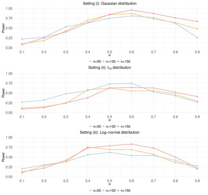
Figure 1 presents the results for Settings (i)-(iii), showing that setting $k=\lfloor\sqrt{n}\rfloor$ achieves satisfactory power across these scenarios. Since the choice of $k$ is not the main focus of this paper, we consistently use $k=\lfloor\sqrt{n}\rfloor$ in the following analysis.

3 Performance analysis

In this section, we compare the performance of GIT-$\text{R}_{\text{r}k\text{NF}}$ with seven other methods: FR1, FR2, dCov, HHG, pCov, IPR, and RdCov, as introduced in Section 1. Our simulation settings encompass a range of distributions to provide a comprehensive evaluation across potential real-world scenarios. In each setting, we generate $X$ and $Y$ samples with their components from (1) Gaussian, (2) $t_{10}$, and (3) log-normal distributions, covering light- to heavy-tailed and symmetric to asymmetric characteristics across low, moderate, and high-dimensional data.

Specifically, we set $\mathcal{X}=\mathcal{Y}=\mathbb{R}^{p}$ with $p\in\{20,100,400,1000\}$ and the sample size $n\in\{50,100,150\}$. We evaluate the empirical power of each method through Settings 1.1 to 4.3, which are constructed under the alternative hypothesis. The nominal level is set as $0.05$. The empirical power is assessed on $200$ replications. The $p$-values for GIT-$\text{R}_{\text{r}k\text{NF}}$ are analytically approximated using Theorem 3 from Section 4, while the $p$-values for the other methods are approximated through $500$ random permutations. Signal and noise levels are chosen so that the best method under each setting has moderate power. In these settings, all observations in $Y$ have one fixed dependency relationship with $X$, except in Settings 3.1 to 3.3, where two dependency structures are used to create complex relationships. The setting details are provided below, with their dependency structures roughly summarized in Table 2.

For $i\in[n],j,l\in[p],Z\in\{X,Y\}$, we obtain $\sigma_{i},\sigma_{i}^{Z}\in\mathbb{R},U_{i},U_{i}^{Z},\epsilon_{i},\epsilon_{i}^{Z},B_{i}^{Z},L_{i}\in\mathbb{R}^{p},\mathbf{\Theta}_{i}=[\Theta_{i,jl}]_{j,l=1}^{p}\in\mathbb{R}^{p\times p}$, by generating $\sigma_{i},\sigma_{i}^{Z},U_{ij},U_{ij}^{Z},\epsilon_{ij},\epsilon_{ij}^{Z},B_{i}^{Z},L_{ij},\Theta_{i,jl}$ independently, except in Settings 4.1 to 4.3 where $\epsilon_{i1}^{Z}=\ldots=\epsilon_{ip}^{Z}$,

  • Setting 1.1: $U_{ij}\sim N(0,1),B_{i}^{X},B_{i}^{Y}\sim\mathrm{Bernoulli}(0.5)$, $\epsilon_{ij}^{X},\epsilon_{ij}^{Y}\sim N(0,1.5^{2})$, $X_{ij}=(-1)^{B_{i}^{X}}$ $\log(|U_{ij}|)+\epsilon_{ij}^{X},Y_{ij}=(-1)^{B_{i}^{Y}}\big{(}5-\log(|U_{ij}|)\big{)}+\epsilon_{ij}^{Y}$.

  • Setting 1.2: $U_{ij}\sim t_{10},B_{i}^{X},B_{i}^{Y}\sim\mathrm{Bernoulli}(0.5)$, $\epsilon_{ij}^{X},\epsilon_{ij}^{Y}\sim 1.5\cdot t_{10}$, $X_{ij}=(-1)^{B_{i}^{X}}$ $\log(|U_{ij}|)+\epsilon_{ij}^{X},Y_{ij}=(-1)^{B_{i}^{Y}}\big{(}5-\log(|U_{ij}|)\big{)}+\epsilon_{ij}^{Y}$.

  • Setting 1.3: $U_{ij}\sim\exp\big(N(-2,1)\big{missing}),B_{i}^{X},B_{i}^{Y}\sim\mathrm{Bernoulli}(0.5)$, $\epsilon_{ij}^{X},\epsilon_{ij}^{Y}\sim\exp\big(N(-0.5,1)\big{missing})$, $X_{j}=(-1)^{B_{i}^{X}}\log(|U_{ij}|)+\epsilon_{ij}^{X},Y_{ij}=(-1)^{B_{i}^{Y}}\big{(}5-\log(|U_{ij}|)\big{)}+\epsilon_{ij}^{Y}$.

  • Setting 2.1: $\sigma_{i}\sim N(0,1),\sigma_{i}^{X},\sigma_{i}^{Y}|\sigma_{i}\sim N(0,\sigma_{i}^{2})$, $U_{ij}^{X}|\sigma_{i}^{X}\sim N\big{(}0,(2-\sigma_{i}^{X})^{2}\big{)},$
    $U_{ij}^{Y}|\sigma_{i}^{Y}\sim N(0,(\sigma_{i}^{Y})^{2})$, $X_{ij}=U_{ij}^{X}+\epsilon_{ij}^{X},Y_{ij}=U_{ij}^{Y}+\epsilon_{ij}^{Y}$, where

    • $\epsilon_{ij}^{X},\epsilon_{ij}^{Y}\sim N(0,0.6^{2})$ for $p=20$,

    • $\epsilon_{ij}^{X},\epsilon_{ij}^{Y}\sim N(0,1)$ for $p\in\{100,400,1000\}$.

  • Setting 2.2: $\sigma_{i}\sim t_{10},\sigma_{i}^{X},\sigma_{i}^{Y}|\sigma_{i}\sim\sigma_{i}t_{10}$, $U_{ij}^{X}|\sigma_{i}^{X}\sim(2-\sigma_{i}^{X})t_{10},U_{ij}^{Y}|\sigma_{i}^{Y}\sim\sigma_{i}^{Y}t_{10}$, $X_{ij}=U_{ij}^{X}+\epsilon_{ij}^{X},Y_{ij}=U_{ij}^{Y}+\epsilon_{ij}^{Y}$, where

    • $\epsilon_{ij}^{X},\epsilon_{ij}^{Y}\sim 0.4\cdot t_{10}$ for $p=20$,

    • $\epsilon_{ij}^{X},\epsilon_{ij}^{Y}\sim t_{10}$ for $p\in\{100,400,1000\}$.

  • Setting 2.3: $\sigma_{i}\sim\exp\big(N(0,1)\big{missing}),\sigma_{i}^{X},\sigma_{i}^{Y}|\sigma_{i}\sim\exp\big(N(0,\sigma_{i}^{2})\big{missing})$, $U_{ij}^{X}|\sigma_{i}^{X}\sim\exp\big(N(0,(5-\sigma_{i}^{X})^{2})\big{missing}),U_{ij}^{Y}|\sigma_{i}^{Y}\sim\exp\big(N(0,(\sigma_{i}^{Y})^{2})\big{missing})$, $X_{ij}=U_{ij}^{X}+\epsilon_{ij}^{X},Y_{ij}=U_{ij}^{Y}+\epsilon_{ij}^{Y}$, where

    • $\epsilon_{ij}^{X},\epsilon_{ij}^{Y}\sim 0.2\cdot\exp\big(N(0,1)\big{missing})$ for $p\in\{20,100,400\}$,

    • $\epsilon_{ij}^{X},\epsilon_{ij}^{Y}\sim 0.1\cdot\exp\big(N(0,1)\big{missing})$ for $p=1000$.

  • Setting 3.1: $X_{ij}\sim N(0,1),\epsilon_{ij}\sim N(0,1.2^{2}),Y_{ij}=\log(|X_{ij}|)+\epsilon_{ij}$ for $i\leq\frac{n}{2}$, $Y_{ij}=\exp(0.6\cdot X_{ij})+\epsilon_{ij}$ for $i>\frac{n}{2}$.

  • Setting 3.2: $X_{ij}\sim t_{10},\epsilon_{ij}\sim t_{10},Y_{ij}=\log(|X_{ij}|)+\epsilon_{ij}$ for $i\leq\frac{n}{2}$, $Y_{ij}=\exp(0.5\cdot X_{ij})+\epsilon_{ij}$ for $i>\frac{n}{2}$.

  • Setting 3.3: $X_{ij}\sim\exp\big(N(-4,1)\big{missing}),$ $Y_{ij}=\log(X_{ij})+\epsilon_{ij}$ for $i\leq\frac{n}{2}$, $Y_{ij}=\exp(0.7\cdot X_{ij})+\epsilon_{ij}$ for $i>\frac{n}{2}$, where

    • $\epsilon_{ij}\sim\exp\big(N(-4,2.9^{2})\big{missing})$ for $p=20$,

    • $\epsilon_{ij}\sim\exp\big(N(-4,2.3^{2})\big{missing})$ for $p=100$,

    • $\epsilon_{ij}\sim\exp\big(N(-4,2^{2})\big{missing})$ for $p\in\{400,1000\}$.

  • Setting 4.1: $L_{ij},\Theta_{i,jl}\sim N(0,1)$, $\epsilon_{i1}^{X},\epsilon_{i1}^{Y}\sim N(0,8^{2}),$ $X_{i}=L_{i}^{\top}\sin\mathbf{\Theta}_{i}+\epsilon_{i}^{X}$, $Y_{i}=L_{i}^{\top}\cos\Theta_{i}$ $+\epsilon_{i}^{Y}$.

  • Setting 4.2: $L_{ij},\Theta_{i,jl}\sim t_{10}$, $\epsilon_{i1}^{X},\epsilon_{i1}^{Y}\sim 10\cdot t_{10},$ $X_{i}=L_{i}^{\top}\sin\mathbf{\Theta}_{i}+\epsilon_{i}^{X}$, $Y_{i}=L_{i}^{\top}\cos\mathbf{\Theta}_{i}+\epsilon_{i}^{Y}$.

  • Setting 4.3: $L_{ij},\Theta_{i,jl}\sim\exp\big(N(0,1)\big{missing})$, $\epsilon_{i1}^{X},\epsilon_{i1}^{Y}\sim\exp(N(0,25^{2})),$ $X_{i}=L_{i}^{\top}\sin\mathbf{\Theta}_{i}+\epsilon_{i}^{X}$, $Y_{i}=L_{i}^{\top}\cos\mathbf{\Theta}_{i}+\epsilon_{i}^{Y}$.

Table 2: Dependency structures in Settings 1.1 to 4.1: Variance (dependent variance among variables); Hierarchical (layered dependency structure); Concatenated (multiple dependency types across samples); Non-monotonic (non-monotonic dependency trends).
Setting Dependency Structure
Variance Hierarchical Concatenated Non-monotonic
1.1-1.3 $\checkmark$ $\checkmark$
2.1-2.3 $\checkmark$ $\checkmark$ $\checkmark$
3.1-3.3 $\checkmark$ $\checkmark$
4.1-4.3 $\checkmark$ $\checkmark$
Refer to caption
Figure 2: Estimated power for Settings 1.1 to 1.3
Refer to caption
Figure 3: Estimated power for Settings 2.1 to 2.3
Refer to caption
Figure 4: Estimated power for Settings 3.1 to 3.3
Refer to caption
Figure 5: Estimated power for Settings 4.1 to 4.3
Refer to caption
Figure 6: Estimated power of components for Settings 4.1

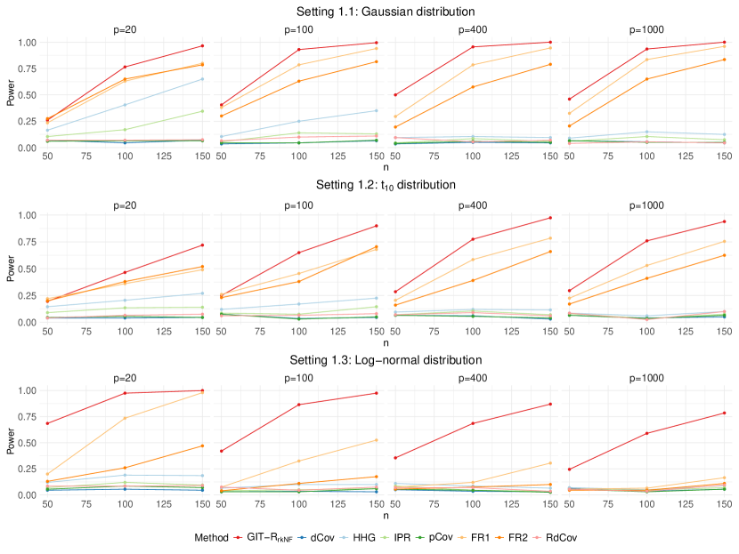
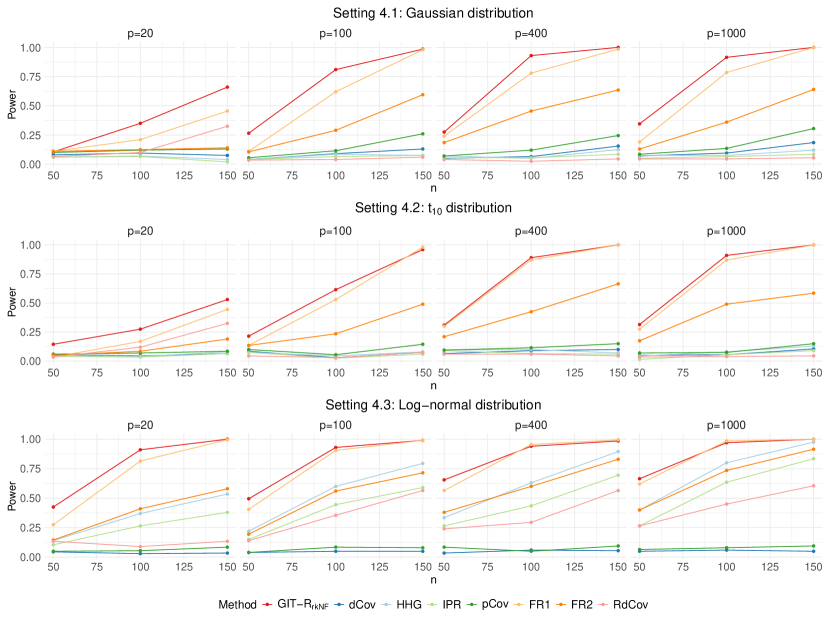
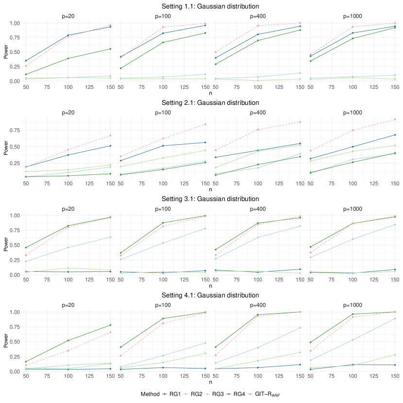
We begin by analyzing the estimated power for Settings 1.1 through 4.3, as shown in Figures 2 to 5. Following this, we examine the contributions of each component in GIT-$\text{R}_{\text{r}k\text{NF}}$ by evaluating the empirical power of the test and its individual components, named by RG1, RG2, RG3, and RG4, which are based on the test statistic

$$\frac{|T_{s}-\mathbb{E}(T_{s})|}{\sqrt{\textup{Var}(T_{s})}},~{}~{}s\in\{1,2,3,4\}.$$

Figure 6 compares these components, highlighting the relative importance of each pairwise relationship for settings generated from Gaussian distributions. Similar results for the other two distributions are provided in Supplement S8.

We first examine the results for Settings 1.1-1.3, as shown in Figure 2. In Setting 1.1 for the Gaussian distribution, GIT-$\text{R}_{\text{r}k\text{NF}}$ exhibits the highest power, with FR1 and FR2 also showing moderate power, while most other methods have negligible power. Notably, HHG maintains moderate power only at $p=20$. For the $t_{10}$ distribution in Setting 1.2, GIT-$\text{R}_{\text{r}k\text{NF}}$ again achieves the highest power, with FR1, and FR2 also showing adequate power. Finally, for the log-normal distribution in Setting 1.3, GIT-$\text{R}_{\text{r}k\text{NF}}$ significantly outperforms all other methods. FR1 and FR2 show moderate power at low dimensions but their power drops sharply at high dimensions.

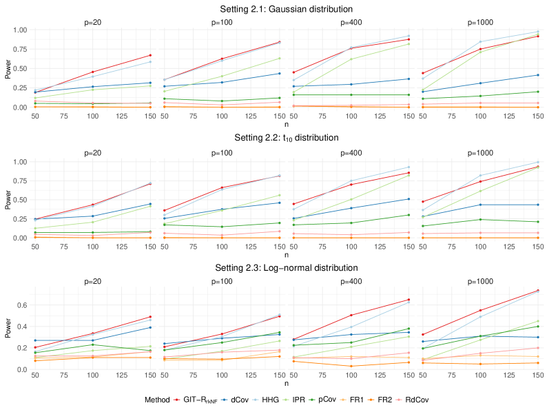
Figure 3 shows the performance for Settings 2.1-2.3. In Setting 2.1 for the Gaussian distribution, GIT-$\text{R}_{\text{r}k\text{NF}}$ performs optimally at $p=20$, followed by HHG. For $p=100,400$ and $1000$, GIT-$\text{R}_{\text{r}k\text{NF}}$ and HHG exhibit superior performance, while IPR also demonstrates satisfactory results. However, other methods show low power in these scenarios. In Setting 2.2 for the $t_{10}$ distribution, GIT-$\text{R}_{\text{r}k\text{NF}}$ and HHG outperform all other methods, while dCov and IPR also perform well for $p=20$. Notably, IPR exhibits satisfactory power for $p=400$ and $1000$, while the power for other methods remains relatively low. In Setting 2.3 for the log-normal distribution, GIT-$\text{R}_{\text{r}k\text{NF}}$ outperforms all other methods, closely followed by HHG.

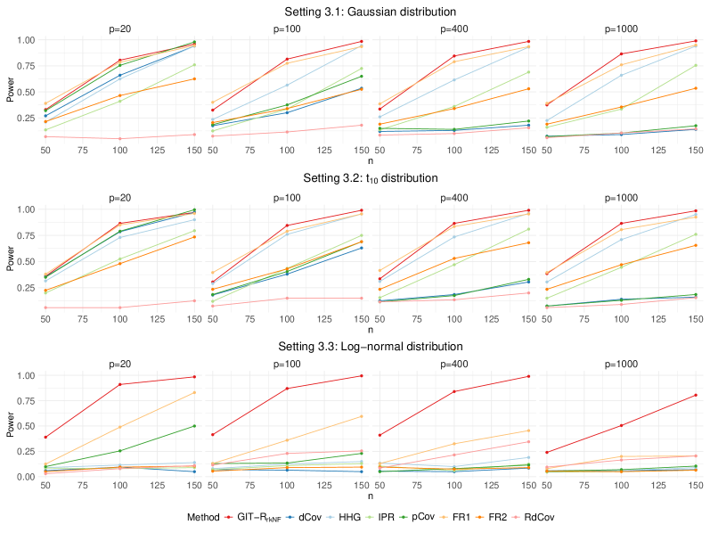
From Figure 4, for the multivariate Gaussian distribution in Setting 3.1, most methods demonstrate satisfactory power, except for RdCov, which has almost no power. As the dimension increases, GIT-$\text{R}_{\text{r}k\text{NF}}$ performs the best, followed closely by FR1, with HHG also showing good power. In Setting 3.2, under the $t_{10}$ distribution, most methods perform well at low dimensions. As the dimension increases, GIT-$\text{R}_{\text{r}k\text{NF}}$ performs the best, followed closely by FR1 and HHG. For the log-normal distribution in Setting 3.3, GIT-$\text{R}_{\text{r}k\text{NF}}$ exhibits outstanding power compared to all other methods across all dimensions. While FR1 and pCov perform moderately well at low dimensions, with FR1 outperforming pCov, their gap in performance relative to GIT-$\text{R}_{\text{r}k\text{NF}}$ widens as the dimension increases.

From Figure 5, we observe that for the multivariate Gaussian distribution in Setting 4.1, GIT-$\text{R}_{\text{r}k\text{NF}}$ performs the best, with FR1 also showing good performance. FR2 achieves about half the power of GIT-$\text{R}_{\text{r}k\text{NF}}$, while the other methods exhibit insufficient power. For the $t_{10}$ distribution in Setting 4.2, GIT-$\text{R}_{\text{r}k\text{NF}}$ and FR1 continue to lead, and followed by FR2. All other methods exhibit negligible power. In Setting 4.3, for the log-normal distribution, GIT-$\text{R}_{\text{r}k\text{NF}}$ and FR1 outperm all other methods, followed by FR2, HHG and IPR.

We now examine the individual components of GIT-$\text{R}_{\text{r}k\text{NF}}$. As shown in Figure 6, RG1 and RG4 are the most influential in Setting 1.1, indicating a dependency involving the alignment of dissimilarity in $X$ with dissimilarity in $Y$, as well as similarity in $X$ with similarity in $Y$. In Setting 2.1, RG1 and RG3 significantly enhance the performance of GIT-$\text{R}_{\text{r}k\text{NF}}$, suggesting that the dependency involves the alignment of dissimilarity in $X$ with dissimilarity in $Y$, and similarity in $X$ with dissimilarity in $Y$. Conversely, in Setting 3.1, RG2 and RG4 are the most impactful, indicating a dependency involving the alignment of dissimilarity in $X$ with similarity in $Y$, and similarity in $X$ with similarity in $Y$. Finally, in Setting 4.1, RG4 merges as the most influential component, highlighting a strong dependency between similarity in $X$ and similarity in $Y$.

In summary, GIT-$\text{R}_{\text{r}k\text{NF}}$ consistently demonstrates superior performance across a variety of distributions and settings, particularly under complex dependency between $X$ and $Y$. FR1 and HHG generally perform well, but their effectiveness is not stable when the dependency becomes complicated. Additionally, FR1 tends to underperform in settings involving high dimensions or log-normal distributions. Based on these comprehensive results, we recommend GIT-$\text{R}_{\text{r}k\text{NF}}$ for its overall effectiveness across diverse settings.

4 Theoretical properties

In this section, we study the asymptotic properties of the test statistic, which are crucial for deriving an analytic approximation of the $p$-value. Recall the test statistic

$$T=(T_{1}-\mu_{1},T_{2}-\mu_{2},T_{3}-\mu_{3},T_{4}-\mu_{4})\mathbf{\Sigma}^{-1}(T_{1}-\mu_{1},T_{2}-\mu_{2},T_{3}-\mu_{3},T_{4}-\mu_{4})^{\top}.$$

We begin by analyzing $T_{s},s=1,2,3,4$, which can be written in the form:

$$T_{s}=\sum_{i=1}^{n}\sum_{j=1}^{n}A_{ij}^{(s)}B_{ij}^{(s)},$$

where $\mathbf{A}^{(1)}=\mathbf{A}^{(2)}=\mathbf{D}^{X}$, $\mathbf{A}^{(3)}=\mathbf{A}^{(4)}=\mathbf{S}^{X}$, $\mathbf{B}^{(1)}=\mathbf{B}^{(3)}=\mathbf{D}^{Y}$ and $\mathbf{B}^{(2)}=\mathbf{B}^{(4)}=\mathbf{S}^{Y}$, with all matrices symmetric and having zero as diagonals. We study their limiting distribution under the permutation null distribution, based on the permuted data $\{(X_{i},Y_{\pi(i)})\}_{i=1}^{n}$, where $\pi$ denotes a permutation of $\{1,\ldots,n\}$ with each permutation equally probable.

4.1 Moment properties

We first derive the analytic expressions for $\mathbb{E}(T_{s})$ and $\textup{Cov}(T_{s},T_{s^{\prime}}),$ $s,s^{\prime}\in\{1,2,3,4\}$ through combinatorial analysis. To simplify the notations, for $\mathbf{C}^{(s)}\in\{\mathbf{A}^{(s)},\mathbf{B}^{(s)}\}$, we denote

$\displaystyle C_{1}^{(s)}=\sum_{i=1}^{n}\sum_{j=1}^{n}C_{ij}^{(s)},\quad C_{i\cdot}^{(s)}=\sum_{j=1}^{n}C_{ij}^{(s)},\text{ for }i\in\{1,\ldots,n\},$
$\displaystyle C_{2}^{(ss^{\prime})}=\sum_{i=1}^{n}\sum_{j=1}^{n}C_{ij}^{(s)}C_{ij}^{(s^{\prime})},\quad C_{3}^{(ss^{\prime})}=\sum_{i=1}^{n}C_{i\cdot}^{(s)}C_{i\cdot}^{(s^{\prime})}.$
Theorem 1.

Under the permutation null distribution, we have that for $s,s^{\prime}\in\{1,2,3,4\}$,

$$\mathbb{E}(T_{s})=\frac{A_{1}^{(s)}B_{1}^{(s)}}{n(n-1)},$$

and

$\displaystyle\textup{Cov}(T_{s},T_{s^{\prime}})=$ $\displaystyle\frac{4(n+1)(A_{3}^{(ss^{\prime})}-\frac{A_{1}^{(s)}A_{1}^{(s^{\prime})}}{n})(B_{3}^{(ss^{\prime})}-\frac{B_{1}^{(s)}B_{1}^{(s^{\prime})}}{n})}{n(n-1)(n-2)(n-3)}$ (4)
$\displaystyle+\frac{2(A_{2}^{(ss^{\prime})}-\frac{A_{1}^{(s)}A_{1}^{(s^{\prime})}}{n(n-1)})(B_{2}^{(ss^{\prime})}-\frac{B_{1}^{(s)}B_{1}^{(s^{\prime})}}{n(n-1)})}{n(n-3)}$
$\displaystyle-\frac{4(A_{2}^{(ss^{\prime})}-\frac{A_{1}^{(s)}A_{1}^{(s^{\prime})}}{n(n-1)})(B_{3}^{(ss^{\prime})}-\frac{B_{1}^{(s)}B_{1}^{(s^{\prime})}}{n})}{n(n-2)(n-3)}$
$\displaystyle-\frac{4(A_{3}^{(ss^{\prime})}-\frac{A_{1}^{(s)}A_{1}^{(s^{\prime})}}{n})(B_{2}^{(ss^{\prime})}-\frac{B_{1}^{(s)}B_{1}^{(s^{\prime})}}{n(n-1)})}{n(n-2)(n-3)}.$

The proof of Theorem 1 is presented in Supplement S1. For the test statistic $T$ to be well-defined, it is crucial that the covariance matrix $\mathbf{\Sigma}$ is positive-definite. This condition is not restrictive and it is feasible to verify the finite-sample positive-definiteness of $\mathbf{\Sigma}$. If ${\rm rank}(\mathbf{\Sigma})<4$, it implies that the statistics $T_{s}$, for $s\in\{1,2,3,4\}$, are linearly dependent. In such cases, using only the linearly independent statistics is sufficient to construct the test statistic. In the following, we will explore the asymptotic distribution of $T_{s}$ under the permutation null distribution and examine the conditions under which $\Sigma$ is asymptotically positive-definite.

4.2 Asymptotic properties

The asymptotic normality of the generalized correlation coefficient, $\Gamma$ (1), has been previously studied by Daniels (1944); Pham, Möcks and Sroka (1989). More recently, Huang and Sen (2024) introduced a novel set of conditions allowing for more flexible scaling relationships than those in Pham, Möcks and Sroka (1989). To understand how these results apply to our statistics $T_{s}$ for $s=1,\dots,4$, we review the conditions in these earlier works. Let $G^{X}$ and $G^{Y}$ represent the similarity or dissimilarity graphs constructed from the $X$ and $Y$ samples, as described in Section 2. We allow $k$ to vary with $n$ such that $k\asymp n^{\alpha}$ for some $\alpha\in[0,1]$. It is important to note that the conditions in Daniels (1944) hold only when $\alpha=1$, and the conditions in Pham, Möcks and Sroka (1989, Theorem 3.2) only apply when $\alpha=0$. However, the conditions in Huang and Sen (2024, Theorem C.1) and Pham, Möcks and Sroka (1989, Theorem 3.1) cannot be satisfied when $\mathbf{A}^{(s)}$ and $\mathbf{B}^{(s)}$ are derived from unweighted graphs or weighted graphs using graph-induced ranks and ranks based on robust graph, as discussed in Supplement 6. Interestingly, as shown in Figure 1, optimal performance of GIT-$\text{R}_{\text{r}k\text{NF}}$ often occurs when $\alpha\in[0.4,0.7]$. Recognizing the gap between $\alpha=0$ and $\alpha=1$, and the practical need for using $\alpha\in(0,1)$, we propose a set of conditions to bridge this gap. Specially, our conditions can potentially be satisfied when $\alpha\in(0,1]$.

We first introduce the following notations. For two sequences of nonnegative real numbers $\{a_{n}\}$ and $\{b_{n}\}$, we denote $a_{n}=o(b_{n})$ or $a_{n}\prec b_{n}$ if $a_{n}$ is dominated by $b_{n}$ asymptotically, i.e., $\lim_{n\rightarrow\infty}a_{n}/b_{n}=0$, $a_{n}\asymp b_{n}$ if $a_{n}$ is bounded both above and below by $b_{n}$ up to a constant factor asymptotically, $a_{n}=O\big{(}b_{n}\big{)}$ or $a_{n}\precsim b_{n}$ if $a_{n}$ is bounded above by $b_{n}$ up to a constant factor asymptotically.

To simplify the derivation, we consider an centered versions of the matrices $\mathbf{C}^{(s)}$, $\mathbf{C}^{(s)}\in\{\mathbf{A}^{(s)},\mathbf{B}^{(s)}\},s\in\{1,2,3,4\}$, such that $\sum_{i=1}^{n}\sum_{j=1}^{n}C_{ij}^{(s)}=0$. If this does not hold, we will replace $C_{ij}^{(s)}$ by $C_{ij}^{(s)}-\frac{C_{1}^{(s)}\mathbb{I}(i\neq j)}{n(n-1)}$, and this centering will not change the value of the generalized test statistic $T$ in (3). Then these centered matrices satisfy the following Condition 1 automatically.

Condition 1.

$C_{ii}^{(s)}=0,C_{ij}^{(s)}=C_{ji}^{(s)},i,j\in\{1,\ldots,n\}$, $C^{(s)}_{1}=0$, for $\mathbf{C}^{(s)}\in\{\mathbf{A}^{(s)},$ $\mathbf{B}^{(s)}\}$ and $s\in\{1,2,3,4\}$.

Let $s^{\prime}\in\{1,2,3,4\}$, we further define

$\displaystyle C^{(s)}_{0+}=\max_{1\leq i,j\leq n}|C^{(s)}_{ij}|,~{}C_{i\star}^{(s)}=\sum_{j=1}^{n}|C_{ij}^{(s)}|,~{}C_{1+}^{(s)}=\max_{1\leq i\leq n}C_{i\star}^{(s)},$
$\displaystyle C_{2+}^{(ss^{\prime})}=\sum_{i=1}^{n}\sum_{j=1}^{n}|C_{ij}^{(s)}C_{ij}^{(s^{\prime})}|,~{}C_{3+}^{(ss^{\prime})}=\sum_{i=1}^{n}|C_{i\star}^{(s)}C_{i\star}^{(s^{\prime})}|.$

Notably, $C_{2+}^{(ss)}=C_{2}^{(ss)}$. We proceed to introduce the following Conditions 2-4. Satisfying any one of these conditions is sufficient for the asymptotic normality of $T_{s}$’s, as stated in Theorem 2. These conditions essentially capture the different dominant terms in the variances associated with each statistic, as shown in Corollary 1.

Condition 2.

$C_{0+}^{(s)}C_{1+}^{(s)}\prec C_{2+}^{(ss)}$, $\max\{n^{2}(A_{0+}^{(s)}B_{0+}^{(s)})^{2},$ $(A_{1+}^{(s)}B_{1+}^{(s)})^{2},$ $n^{-1}A_{3+}^{(ss)}B_{3+}^{(ss)}\}$
$\prec A_{2+}^{(ss)}B_{2+}^{(ss)}$.

Condition 3.

$\max\{n^{3}(A_{0+}^{(s)}B_{0+}^{(s)})^{2},$ $n(A_{1+}^{(s)}B_{1+}^{(s)})^{2},$ $nA_{2+}^{(ss)}B_{2+}^{(ss)}\}\prec A_{3+}^{(ss)}B_{3+}^{(ss)}$ $\asymp~{}~{}$ $A_{3}^{(ss)}B_{3}^{(ss)}$.

Condition 4.

$C_{0+}^{(s)}C_{1+}^{(s)}\prec C_{2+}^{(ss)}\prec C_{3+}^{(ss)}$, $\max\{n^{3}(A_{0+}^{(s)}B_{0+}^{(s)})^{2},n(A_{1+}^{(s)}B_{1+}^{(s)})^{2}\}\prec~{}~{}$ $nA_{2+}^{(ss)}B_{2+}^{(ss)}$ $\asymp A_{3+}^{(ss)}B_{3+}^{(ss)}$ $\asymp A_{3}^{(ss)}B_{3}^{(ss)}$.

Theorem 2.

Assume that $\mathbf{A}^{(s)}$ and $\mathbf{B}^{(s)}$ satisfy Condition 1. If $\mathbf{A}^{(s)}$ and $\mathbf{B}^{(s)}$ further satisfy one of Conditions 2-4, we then have

$$\frac{T_{s}}{\sqrt{{\rm Var}(T_{s})}}\stackrel{{\scriptstyle\mathcal{D}}}{{\rightarrow}}N(0,1)~{}\text{ when }n\rightarrow\infty$$ (5)

under the permutation null distribution, where $\stackrel{{\scriptstyle\mathcal{D}}}{{\rightarrow}}$ denotes convergence in distribution.

The proof of Theorem 2 is provided in Supplement S2. This proof predominantly utilizes the technique of moments matching, a method that has been crucial in showing the asymptotic behavior for the double-indexed linear permutation statistics including graph-based statistics (Henze, 1988; Petrie, 2016; Huang and Sen, 2024) and kernel-based statistics (Song and Chen, 2023a, b). However, we introduce a novel approach to bound the terms in the high-order moments of $T_{s}$, which simplifies the problem to controlling the orders of the terms $C_{0+}^{(s)},C_{1+}^{(s)},C_{2+}^{(ss)},$ and $C_{3+}^{(ss)}$. Furthermore, Conditions 2-4 illustrate how different scaling conditions can influence the dominant terms in the asymptotic variance of $T_{s}$, as shown by Corollary 1.

Corollary 1.

If $\mathbf{A}^{(s)}$ and $\mathbf{B}^{(s)}$ satisfy Conditions 1 and 2, we have

$$\lim_{n\rightarrow\infty}\frac{{\rm Var}(T_{s})}{2n^{-2}A_{2}^{(ss)}B_{2}^{(ss)}}=1.$$

If $\mathbf{A}^{(s)}$ and $\mathbf{B}^{(s)}$ satisfy Conditions 1 and 3, we have

$$\lim_{n\rightarrow\infty}\frac{{\rm Var}(T_{s})}{4n^{-3}A_{3}^{(ss)}B_{3}^{(ss)}}=1.$$

If $\mathbf{A}^{(s)}$ and $\mathbf{B}^{(s)}$ satisfy Conditions 1 and 4, we have

$$\lim_{n\rightarrow\infty}\frac{{\rm Var}(T_{s})}{2n^{-2}A_{2}^{(ss)}B_{2}^{(ss)}+4n^{-3}A_{3}^{(ss)}B_{3}^{(ss)}}=1.$$
Remark 1.

To better understand Conditions 2-4, we simplify the choice of graphs and restate the conditions under these simplified graphs in Tables 3 and 4.

Table 3: Some scenarios satisfying Conditions 2-4 for unweighted graphs (Example 1), assuming $k\asymp n^{\alpha}$, $\max_{i}|G_{i}^{X}|\asymp$ $\max_{i}|G_{i}^{Y}|\asymp$ $n^{\beta}\lesssim n$ and $C_{3+}\asymp n^{\nu}$, where $|G_{i}^{X}|$ and $|G_{i}^{Y}|$ are degrees of $i$-th node in graphs $G^{X}$ and $G^{Y}$. We also assume $C_{3}\asymp n^{\nu}$ in Conditions 3 and 4.
Condition $0\leq\alpha\leq 1$ $\alpha\leq\beta\leq 1$ $1+2\alpha\leq\nu\leq 1+\alpha+\beta$
Condition 2 $0<\alpha<\frac{1}{2}$ $\beta<\frac{1+\alpha}{2}$ $\nu<\frac{3}{2}+\alpha$
Condition 3 $0<\alpha\leq 1$ $\beta<\frac{\nu}{2}-\frac{1}{4}$ $\nu>\frac{3}{2}+\alpha$
Condition 4 $0<\alpha\leq\frac{1}{2}$ $\beta<\frac{1+\alpha}{2}=\frac{\nu}{2}-\frac{1}{4}$ $\nu=\frac{3}{2}+\alpha$
Table 4: Some scenarios satisfying Conditions 2-4 for weighted graphs with graph-induced ranks (Example 4) or ranks based on robust graph (Example 5), assuming $k\asymp n^{\alpha}$, $A_{1+}\asymp B_{1+}\asymp n^{\beta}\lesssim nk$ and $C_{3+}\asymp n^{\nu}$. We also assume $C_{3}\asymp n^{\nu}$ in Conditions 3 and 4.
Condition $0\leq\alpha\leq 1$ $2\alpha\leq\beta\leq 1+\alpha$ $1+4\alpha\leq\nu\leq 1+2\alpha+\beta$
Condition 2 $0<\alpha<\frac{1}{2}$ $\beta<\frac{1+3\alpha}{2}$ $\nu<\frac{3}{2}+3\alpha$
Condition 3 $0<\alpha\leq 1$ $\beta<\frac{\nu}{2}-\frac{1}{4}$ $\nu>\frac{3}{2}+3\alpha$
Condition 4 $0<\alpha\leq\frac{1}{2}$ $\beta<\frac{1+3\alpha}{2}=\frac{\nu}{2}-\frac{1}{4}$ $\nu=\frac{3}{2}+3\alpha$

In addition to the asymptotic distribution of $\Gamma_{s},s\in\{1,2,3,4\}$, we also consider the joint distribution of $(\Gamma_{1},\Gamma_{2},\Gamma_{3},\Gamma_{4})$. We proceed by introducing the following Conditions 5-7. For the asymptotic properties in Theorem 3, only one of these conditions needs to be satisfied. For each condition, it needs to hold simultaneously for all pairs $s,s^{\prime}\in\{1,2,3,4\}$ with $s\neq s^{\prime}$.

Condition 5.

$A_{2+}^{(ss^{\prime})},B_{2+}^{(ss^{\prime})}$ satisfy either $|A_{2}^{(ss^{\prime})}|\asymp A_{2+}^{(ss^{\prime})}$, $|B_{2}^{(ss^{\prime})}|\asymp B_{2+}^{(ss^{\prime})}$, or $A_{2+}^{(ss^{\prime})}\prec\sqrt{A_{2+}^{(ss)}A_{2+}^{(s^{\prime}s^{\prime})}}$, $B_{2+}^{(ss^{\prime})}\prec\sqrt{B_{2+}^{(ss)}B_{2+}^{(s^{\prime}s^{\prime})}}$, and $C_{0+}^{(s)}$, $C_{1+}^{(s)},$ $C_{2+}^{(ss)},$ $C_{3+}^{(ss)}$ satisfy Condition 2, with $\mathbf{C}^{(s)}\in\{\mathbf{A}^{(s)},\mathbf{B}^{(s)}\}$.

Condition 6.

$A_{3+}^{(ss^{\prime})},B_{3+}^{(ss^{\prime})}$ satisfy either $|A_{3}^{(ss^{\prime})}|\asymp A_{3+}^{(ss^{\prime})}$, $|B_{3}^{(ss^{\prime})}|\asymp B_{3+}^{(ss^{\prime})}$, or $A_{3+}^{(ss^{\prime})}\prec\sqrt{A_{3+}^{(ss)}A_{3+}^{(s^{\prime}s^{\prime})}}$, $A_{3+}^{(ss^{\prime})}\prec\sqrt{A_{3+}^{(ss)}A_{3+}^{(s^{\prime}s^{\prime})}}$, and $C_{0+}^{(s)}$, $C_{1+}^{(s)},$ $C_{2+}^{(ss)},$ $C_{3+}^{(ss)}$ satisfy Condition 3, with $\mathbf{C}^{(s)}\in\{\mathbf{A}^{(s)},\mathbf{B}^{(s)}\}$.

Condition 7.

$A_{2+}^{(ss^{\prime})}$, $B_{2+}^{(ss^{\prime})}$, $A_{3+}^{(ss^{\prime})}$, $B_{3+}^{(ss^{\prime})}$ satisfy either $|A_{2}^{(ss^{\prime})}|\asymp A_{2+}^{(ss^{\prime})}$, $|B_{2}^{(ss^{\prime})}|\asymp B_{2+}^{(ss^{\prime})}$, $|A_{3}^{(ss^{\prime})}|\asymp A_{3+}^{(ss^{\prime})}$, $|B_{3}^{(ss^{\prime})}|\asymp B_{3+}^{(ss^{\prime})}$, or $A_{2+}^{(ss^{\prime})}\prec\sqrt{A_{2+}^{(ss)}A_{2+}^{(s^{\prime}s^{\prime})}}$, $B_{2+}^{(ss^{\prime})}\prec\sqrt{B_{2+}^{(ss)}B_{2+}^{(s^{\prime}s^{\prime})}}$, $A_{3+}^{(ss^{\prime})}\prec\sqrt{A_{3+}^{(ss)}A_{3+}^{(s^{\prime}s^{\prime})}}$, $B_{3+}^{(ss^{\prime})}\prec\sqrt{B_{3+}^{(ss)}B_{3+}^{(s^{\prime}s^{\prime})}}$, and $C_{0+}^{(s)}$, $C_{1+}^{(s)},$ $C_{2+}^{(ss)},$ $C_{3+}^{(ss)}$ satisfy Condition 4, with $\mathbf{C}^{(s)}\in\{\mathbf{A}^{(s)},\mathbf{B}^{(s)}\}$.

Theorem 3.

Assume that $\mathbf{A}^{(s)}$ and $\mathbf{B}^{(s)}$ for $s\in\{1,2,3,4\}$ satisfy Condition 1. If $\mathbf{A}^{(s)}$ and $\mathbf{B}^{(s)}$ further satisfy one of Conditions 5-7, and if $\textup{Cov}\big{(}(T_{1},T_{2},T_{3},T_{4})^{\top}\big{)}$ is invertible, then we have

$\displaystyle(T_{1},T_{2},T_{3},T_{4})\textup{Cov}^{-1}\big{(}(T_{1},T_{2},T_{3},T_{4})^{\top}\big{)}(T_{1},T_{2},T_{3},T_{4})^{\top}\stackrel{{\scriptstyle\mathcal{D}}}{{\rightarrow}}\chi_{4}^{2},$ (6)

under the permutation null distribution.

The proof of Theorem 3 is provided in Supplement S3, and discussions about the invertibility of $\textup{Cov}\big{(}(T_{1},T_{2},T_{3},T_{4})^{\top}\big{)}$ are detailed in Theorem 4.

All of Conditions 5-7 imply that the correlation can be $O(1)$ or $o(1)$ for $T_{s},T_{s^{\prime}}$ with $s\neq s^{\prime}$. Take Condition 5 as an example. The correlation $\textup{Cov}(T_{s},T_{s^{\prime}})/\sqrt{\textup{Var}(T_{s})\textup{Var}(T_{s^{\prime}})}$ is either $o(1)$ or dominated by

$$A_{2}^{(ss^{\prime})}B_{2}^{(ss^{\prime})}/\sqrt{A_{2}^{(ss)}B_{2}^{(ss)}A_{2}^{(s^{\prime}s^{\prime})}B_{2}^{(s^{\prime}s^{\prime})}},$$

which may be of order $O(1)$ when $|A_{2}^{(ss^{\prime})}|\asymp A_{2+}^{(ss^{\prime})}$, $|B_{2}^{(ss^{\prime})}|\asymp B_{2+}^{(ss^{\prime})}$, but will be of order $o(1)$ when $|A_{2}^{(ss^{\prime})}|\prec A_{2+}^{(ss^{\prime})}$, $|B_{2}^{(ss^{\prime})}|\prec B_{2+}^{(ss^{\prime})}$.

Regarding the joint normality of multiple double-indexed permutation statistics, to the best of our knowledge, only Daniels (1944) has investigated the asymptotic behavior of bivariate double-indexed permutation statistics. In Daniels (1944), it is required that $|A_{3}^{(ss^{\prime})}|$ be of order $n^{3}A_{0+}^{(s)}A_{0+}^{(s^{\prime})}$ and $|B_{3}^{(ss^{\prime})}|$ be of order $n^{3}B_{0+}^{(s)}B_{0+}^{(s^{\prime})}$ for $s\leq s^{\prime},s,s^{\prime}\in\{1,2\}$. These are much stronger conditions compared to Condition 6. To see this, note that it can be shown that $|C_{3}^{(ss^{\prime})}|\leq C_{3+}^{(ss^{\prime})}\leq n^{3}C_{0+}^{(s)}C_{0+}^{(s^{\prime})}$, where $\mathbf{C}^{(s)}\in\{\mathbf{A}^{(s)},\mathbf{B}^{(s)}\}$ and $s$ and $s^{\prime}$ can be the same. Thus, $|C_{3}^{(ss^{\prime})}|\asymp n^{3}C_{0+}^{(s)}C_{0+}^{(s^{\prime})}$ implies $|C_{3}^{(ss^{\prime})}|\asymp C_{3+}^{(ss^{\prime})}\asymp n^{3}C_{0+}^{(s)}C_{0+}^{(s^{\prime})}$. By similar reasoning, we have $A_{3+}^{(ss)}B_{3+}^{(ss)}\asymp n^{6}(A_{0+}^{(s)}B_{0+}^{(s)})^{2}$, and it is straightforward to show that $n^{6}(A_{0+}^{(s)}B_{0+}^{(s)})^{2}$ exceeds the order of $\max\{n^{3}(A_{0+}^{(s)}B_{0+}^{(s)})^{2},$ $n(A_{1+}^{(s)}B_{1+}^{(s)})^{2},$ $nA_{2+}^{(ss)}B_{2+}^{(ss)}\}$. Therefore, Condition 6 is much more relaxed than the conditions in Daniels (1944). Moreover, in our case, satisfying any one of Conditions 5, 6, or 7 is sufficient. Additionally, Daniels (1944) restricts $\alpha=1$, whereas our conditions allow for $\alpha\in(0,1]$. Furthermore, Daniels (1944) restricts $\textup{Corr}(T_{1},T_{2})$ to be of order $1$, while our conditions permit $\textup{Corr}(T_{1},T_{2})$ to be either of order $1$ or $o(1)$. Overall, our framework offers greater generality for joint normality compared to Daniels (1944).

We proceed to consider the asymptotic invertibility of $\textup{Cov}\big{(}(T_{1},T_{2},T_{3},T_{4})^{\top}\big{)}$. Given four matrices or vectors $\mathbf{H}^{(1)},\mathbf{H}^{(2)},\mathbf{H}^{(3)},\mathbf{H}^{(4)}$ with $\|\mathbf{H}^{(s)}\|=1$, where $\|\cdot\|$ denotes the Frobenius norm when $\mathbf{H}^{(s)}$ is a matrix and the Euclidean norm when $\mathbf{H}^{(s)}$ is a vector, we will say that they are asymptotically linearly independent if they satisfy the following condition: there do not exist sequences $\{a_{s}(n)\}$ for $s\in\{1,2,3,4\}$ such that

$$\lim_{n\rightarrow\infty}\Big{\|}\sum_{s=1}^{4}a_{s}(n)\mathbf{H}^{(s)}\Big{\|}^{2}=0~{}\text{ where }\max_{s\in\{1,2,3,4\}}\lim_{n\rightarrow\infty}|a_{s}(n)|>0.$$
Theorem 4.

$\textup{Cov}\big{(}(T_{1},T_{2},T_{3},T_{4})^{\top}\big{)}$ is asymptotically invertible if and only if:

  • Under Condition 5 or 7, the four of $\tilde{A}_{2}^{(1)}(\tilde{B}_{2}^{(1)})^{\top}$, $\tilde{A}_{2}^{(2)}(\tilde{B}_{2}^{(2)})^{\top}$, $\tilde{A}_{2}^{(3)}(\tilde{B}_{2}^{(3)})^{\top}$, $\tilde{A}_{2}^{(4)}(\tilde{B}_{2}^{(4)})^{\top}$ are asymptotically linearly independent, where

    $$\tilde{C}_{2}^{(s)}=\big{(}C_{2}^{(ss)}\big{)}^{-\frac{1}{2}}(C_{11}^{(s)},C_{12}^{(s)},\ldots,C_{nn}^{(s)})\in\mathbb{R}^{n^{2}},$$

    for $\mathbf{C}^{(s)}\in\{\mathbf{A}^{(s)},\mathbf{B}^{(s)}\},s\in\{1,2,3,4\}$.

  • Under Condition 6, the four of $\tilde{A}_{3}^{(1)}(\tilde{B}_{3}^{(1)})^{\top}$, $\tilde{A}_{3}^{(2)}(\tilde{B}_{3}^{(2)})^{\top}$, $\tilde{A}_{3}^{(3)}(\tilde{B}_{3}^{(3)})^{\top}$, $\tilde{A}_{3}^{(4)}(\tilde{B}_{3}^{(4)})^{\top}$ are asymptotically linearly independent, where

    $\displaystyle\tilde{C}_{3}^{(s)}=\big{(}C_{3}^{(ss)}\big{)}^{-\frac{1}{2}}(C_{1.}^{(s)},\ldots,C_{n.}^{(s)})\in\mathbb{R}^{n},$ (7)

    for $\mathbf{C}^{(s)}\in\{\mathbf{A}^{(s)},\mathbf{B}^{(s)}\},s\in\{1,2,3,4\}$.

The proof of Theorem 4 is provided in Supplement S4. Additionally, we present two corollaries that provide sufficient conditions when $\tilde{A}_{2}^{(s)}$ and $\tilde{B}_{2}^{(s)}$ are considered separately, with their proofs also included in Supplement S4.

Corollary 2.

$\textup{Cov}\big{(}(T_{1},T_{2},T_{3},T_{4})^{\top}\big{)}$ is asymptotically invertible if:

  • Under Condition 5 or 7, either the four of $\tilde{A}_{2}^{(1)},\tilde{A}_{2}^{(2)},\tilde{A}_{2}^{(3)},\tilde{A}_{2}^{(4)}$ or the four of $\tilde{B}_{2}^{(1)},$ $\tilde{B}_{2}^{(2)},$ $\tilde{B}_{2}^{(3)},$ $\tilde{B}_{2}^{(4)}$ are asymptotically linearly independent.

  • Under Condition 6, either the four of $\tilde{A}_{3}^{(1)},\tilde{A}_{3}^{(2)},\tilde{A}_{3}^{(3)},\tilde{A}_{3}^{(4)}$ or the four of $\tilde{B}_{3}^{(1)},$ $\tilde{B}_{3}^{(2)},$ $\tilde{B}_{3}^{(3)},$ $\tilde{B}_{3}^{(4)}$ are asymptotically linearly independent.

Corollary 3.

In our test statistic in (3), with $\mathbf{A}^{(1)}=\mathbf{A}^{(2)}$, $\mathbf{A}^{(3)}=\mathbf{A}^{(4)}$, $\mathbf{B}^{(1)}=\mathbf{B}^{(3)}$, $\mathbf{B}^{(2)}=\mathbf{B}^{(4)}$, $\textup{Cov}\big{(}(T_{1},T_{2},T_{3},T_{4})^{\top}\big{)}$ is asymptotically invertible if and only if:

  • Under Condition 5 or 7, $\tilde{A}_{2}^{(1)}$ and $\tilde{A}_{2}^{(3)}$ are asymptotically linearly independent, and $\tilde{B}_{2}^{(1)}$ and $\tilde{B}_{2}^{(2)}$ are asymptotically linearly independent.

  • Under Condition 6, $\tilde{A}_{3}^{(1)}$ and $\tilde{A}_{3}^{(3)}$ are asymptotically linearly independent, and $\tilde{B}_{3}^{(1)}$ and $\tilde{B}_{3}^{(2)}$ are asymptotically linearly independent.

Next, we evaluate the analytic $p$-value approximation based on the limiting distribution in Theorem 3. Specifically, we examine the empirical size of GIT-$\text{R}_{\text{r}k\text{NF}}$ when $X$ and $Y$ are independent. The empirical size is calculated from $500$ replications, with $p$-values computed analytically using Theorem 3. We consider dimensions $p\in\{20,100,400,1000\}$ and sample sizes $n\in\{50,100,150\}$, for $i\in[n],j\in[p]$ in the following settings:

  • Setting 5.1: $X_{ij},Y_{ij}\overset{iid}{\sim}N(0,1)$.

  • Setting 5.2: $X_{ij},Y_{ij}\overset{iid}{\sim}t_{10}$.

  • Setting 5.3: $X_{ij},Y_{ij}\overset{iid}{\sim}\exp\big(N(0,1)\big{missing})$.

The empirical sizes for Settings 5.1 to 5.3 are presented in Table 5. The results show that the empirical size of GIT-$\text{R}_{\text{r}k\text{NF}}$ is reasonably well controlled across different distributions and dimensions.

Table 5: Empirical sizes of GIT-$\text{R}_{\text{r}k\text{NF}}$ at 0.05 significance level for Settings 5.1, 5.2, and 5.3.
$p$ Setting 5.1 Setting 5.2 Setting 5.3
$n=50$ $n=100$ $n=150$ $n=50$ $n=100$ $n=150$ $n=50$ $n=100$ $n=150$
20 0.046 0.058 0.056 0.032 0.054 0.060 0.054 0.052 0.052
100 0.050 0.054 0.046 0.042 0.046 0.052 0.046 0.038 0.046
400 0.030 0.050 0.066 0.068 0.044 0.044 0.058 0.056 0.042
1000 0.066 0.048 0.052 0.042 0.040 0.058 0.056 0.052 0.046

5 Real data analysis

The Genotype-Tissue Expression (GTEx) project is a pioneering genomics initiative aimed at exploring the relationship between genetic variation and gene expression in humans. To illustrate the proposed tests, we analyze gene expression data from GTExPortal (version V8)222https://www.gtexportal.org/home/datasets. Previous analyses have primarily focused on the association between tissues (Urbut et al., 2019; Zhou et al., 2020; Khunsriraksakul et al., 2022). In this section, we aim to provide robust statistical evidence of the dependence relationships between gene expressions in two specific tissues.

The dataset used in our study is from Khunsriraksakul et al. (2022), which has been adjusted for several covariates, including sex, sequencing platform, the top three genetic principal components, and probabilistic estimation of expression residuals (PEER) factors. The question of whether the human tumor virus, Epstein–Barr Virus (EBV), promotes breast cancer remains unresolved, and the mechanisms involved are still not fully understood (Hu et al., 2016; Arias-Calvachi et al., 2022). Our analysis focuses on testing the independence of gene expressions between breast mammary cells and EBV-transformed lymphocytes, using $66$ common samples. The number of gene expressions analyzed totals $25,849$ for breast mammary cells and $22,759$ for EBV-transformed lymphocytes.

To evaluate our method GIT-$\text{R}_{\text{r}k\text{NF}}$, we compare it against other methods shown to be effective in simulation studies, including dCov, HHG, IPR, FR1, and FR2. We conducted $1,000$ permutations the compared methods to estimate the $p$-values, which are summarized in Table 6.

Table 6: The $p$-values of different methods.
GIT-$\text{R}_{\text{r}k\text{NF}}$ dCov HHG IPR FR1 FR2
$p$-value $\mathbf{0.005}$ 0.334 0.513 0.617 0.769 0.879

From Table 6, it is evident that GIT-$\text{R}_{\text{r}k\text{NF}}$ successfully detects dependency between breast mammary cells and EBV-transformed lymphocytes at the $0.05$ nominal level, with an approximate $p$-value of $0.005$. This result aligns with some findings in biological literature. Hu et al. (2016) showed that mammary epithelial cells (MECs) express CD21 and can be infected by EBV, and EBV infection of MECs leads to changes in gene expression. The data-driven covariance matrix with largest mash weight in Urbut et al. (2019) showed that there is a strong correlation between breast mammary and cells EBV-transformed lymphocytes. In contrast, the other competing methods fail to identify this dependency. This further validates that our method can capture complicated relationships between two random vectors and uncover meaningful relationships in real-world datasets.

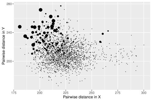
To further investigate the contributions from different components, we analyze RG1 through RG4 to assess the pairwise distance relationships between observations of $X$ and observations of $Y$ that contribute to the significance of GIT-$\text{R}_{\text{r}k\text{NF}}$. From Table 7, we can see that among the four components of GIT-$\text{R}_{\text{r}k\text{NF}}$, only RG3 shows a significant result, with an approximate $p$-value of $0.006$.

Table 7: The $p$-values of RG1-RG4.
RG1 RG2 RG3 RG4
$p$-value 0.192 0.326 $\mathbf{0.006}$ 0.690

The effectiveness of RG3 and GIT-$\text{R}_{\text{r}k\text{NF}}$ is illustrated in Figure 7, which depicts pairwise distances between $X$ and $Y$, for paired samples that are connected in both similarity graph of $X$ and dissimilarity graph of $Y$. The figure suggests a reverse relationship between the pairwise distances in $X$ and those in $Y$, a dynamic often missed by traditional distance-based methods.

Additionally, we compute the analytic $p$-value approximation for GIT-$\text{R}_{\text{r}k\text{NF}}$, which yields 0.008, closely matching the permutation $p$-value. This result is reassuring, as it supports the accuracy of the analytic $p$-value approximation for small $p$-values, even with a modest sample size of 66.

Refer to caption
Figure 7: Scatter plot of pairwise distances in $X$ and $Y$, with point size represents the magnitude of $S_{ij}^{X}D_{ij}^{Y}/25$, rounded to the nearest integer.

6 Discussion

In our test statistic $T$, we combine information from $T_{s}$ for $s\in\{1,2,3,4\}$. However, it may not always be necessary to consider all components simultaneously. For instance, if the focus is on a specific type of dependence, one could use a standardized statistic:

$$\widetilde{T}_{s}=\frac{T_{s}-\mathbb{E}(T_{s})}{\sqrt{\textup{Var}(T_{s})}},$$

for a particular $s\in\{1,2,3,4\}$. Alternatively, the test statistic could be the maximum:

$$M=\max\big{\{}|\widetilde{T}_{1}|,|\widetilde{T}_{2}|,|\widetilde{T}_{3}|,|\widetilde{T}_{4}|\big{\}}.$$

Exploring these alternative test statistics will be left for future work. Additionally, we may also investigate a date-driven approach to selecting the optimal $k$ when constructing the similarity and dissimilarity graphs.

Finally, we emphasize our theoretical contribution in relaxing the conditions required for the asymptotic normality of the double-indexed statistic $T_{s}$. This relaxation may have significant implications for various statistical problems, including distance covariance (Park, Shao and Yao, 2015; Székely and Rizzo, 2014), multivariate two-sample test statistics (Friedman and Rafsky, 1979; Schilling, 1986) and spatial statistics (Mantel, 1967; Kashlak and Yuan, 2022). For instance, our theoretical framework could extend the work of Huang and Sen (2024) to allow for denser graphs when estimating kernel-based measures of dissimilarity between distributions.

{acks}

[Acknowledgments] Mingshuo Liu and Hao Chen are supported in part by NSF award DMS-2311399. Doudou Zhou is supported in part by NUS Start-up Grant A-0009985-00-00. We are grateful to Lida Wang for generously providing the data for the Genotype-Tissue Expression analysis, and we thank Wei Zhong for kindly sharing the code for the pCov method.

References

  • Arias-Calvachi et al. (2022) {barticle}[author] \bauthor\bsnmArias-Calvachi, \bfnmClaudia\binitsC., \bauthor\bsnmBlanco, \bfnmRancés\binitsR., \bauthor\bsnmCalaf, \bfnmGloria M\binitsG. M. and \bauthor\bsnmAguayo, \bfnmFrancisco\binitsF. (\byear2022). \btitleEpstein–Barr virus association with breast cancer: evidence and perspectives. \bjournalBiology \bvolume11 \bpages799. \endbibitem
  • Bergsma and Dassios (2014) {barticle}[author] \bauthor\bsnmBergsma, \bfnmWicher\binitsW. and \bauthor\bsnmDassios, \bfnmAngelos\binitsA. (\byear2014). \btitleA consistent test of independence based on a sign covariance related to Kendall’s tau. \bjournalBernoulli \bvolume20 \bpages1006–1028. \endbibitem
  • Berrett and Samworth (2019) {barticle}[author] \bauthor\bsnmBerrett, \bfnmThomas B\binitsT. B. and \bauthor\bsnmSamworth, \bfnmRichard J\binitsR. J. (\byear2019). \btitleNonparametric independence testing via mutual information. \bjournalBiometrika \bvolume106 \bpages547–566. \endbibitem
  • Biswas, Sarkar and Ghosh (2016) {barticle}[author] \bauthor\bsnmBiswas, \bfnmMunmun\binitsM., \bauthor\bsnmSarkar, \bfnmSoham\binitsS. and \bauthor\bsnmGhosh, \bfnmAnil K\binitsA. K. (\byear2016). \btitleOn some exact distribution-free tests of independence between two random vectors of arbitrary dimensions. \bjournalJournal of Statistical Planning and Inference \bvolume175 \bpages78–86. \endbibitem
  • Blum, Kiefer and Rosenblatt (1961) {barticle}[author] \bauthor\bsnmBlum, \bfnmJ. R.\binitsJ. R., \bauthor\bsnmKiefer, \bfnmJ.\binitsJ. and \bauthor\bsnmRosenblatt, \bfnmM.\binitsM. (\byear1961). \btitleDistribution Free Tests of Independence Based on the Sample Distribution Function. \bjournalThe Annals of Mathematical Statistics \bvolume32 \bpages485 – 498. \bdoi10.1214/aoms/1177705055 \endbibitem
  • Cai, Lei and Roeder (2023) {barticle}[author] \bauthor\bsnmCai, \bfnmZhanrui\binitsZ., \bauthor\bsnmLei, \bfnmJing\binitsJ. and \bauthor\bsnmRoeder, \bfnmKathryn\binitsK. (\byear2023). \btitleAsymptotic Distribution-Free Independence Test for High-Dimension Data. \bjournalJournal of the American Statistical Association \bvolume0 \bpages1–21. \endbibitem
  • Chatterjee (2021) {barticle}[author] \bauthor\bsnmChatterjee, \bfnmSourav\binitsS. (\byear2021). \btitleA new coefficient of correlation. \bjournalJournal of the American Statistical Association \bvolume116 \bpages2009–2022. \endbibitem
  • Daniels (1944) {barticle}[author] \bauthor\bsnmDaniels, \bfnmHenry E\binitsH. E. (\byear1944). \btitleThe relation between measures of correlation in the universe of sample permutations. \bjournalBiometrika \bvolume33 \bpages129–135. \endbibitem
  • Deb and Sen (2023) {barticle}[author] \bauthor\bsnmDeb, \bfnmNabarun\binitsN. and \bauthor\bsnmSen, \bfnmBodhisattva\binitsB. (\byear2023). \btitleMultivariate Rank-Based Distribution-Free Nonparametric Testing Using Measure Transportation. \bjournalJournal of the American Statistical Association \bvolume118 \bpages192–207. \endbibitem
  • Feige and Pearce (1979) {barticle}[author] \bauthor\bsnmFeige, \bfnmEdgar L\binitsE. L. and \bauthor\bsnmPearce, \bfnmDouglas K\binitsD. K. (\byear1979). \btitleThe casual causal relationship between money and income: Some caveats for time series analysis. \bjournalThe Review of Economics and Statistics \bpages521–533. \endbibitem
  • Friedman and Rafsky (1979) {barticle}[author] \bauthor\bsnmFriedman, \bfnmJerome H.\binitsJ. H. and \bauthor\bsnmRafsky, \bfnmLawrence C.\binitsL. C. (\byear1979). \btitleMultivariate Generalizations of the Wald-Wolfowitz and Smirnov Two-Sample Tests. \bjournalThe Annals of Statistics \bvolume7 \bpages697–717. \endbibitem
  • Friedman and Rafsky (1983) {barticle}[author] \bauthor\bsnmFriedman, \bfnmJerome H.\binitsJ. H. and \bauthor\bsnmRafsky, \bfnmLawrence C.\binitsL. C. (\byear1983). \btitleGraph-Theoretic Measures of Multivariate Association and Prediction. \bjournalThe Annals of Statistics \bvolume11 \bpages377–391. \endbibitem
  • Gretton et al. (2007) {binproceedings}[author] \bauthor\bsnmGretton, \bfnmArthur\binitsA., \bauthor\bsnmFukumizu, \bfnmKenji\binitsK., \bauthor\bsnmTeo, \bfnmChoon\binitsC., \bauthor\bsnmSong, \bfnmLe\binitsL., \bauthor\bsnmSchölkopf, \bfnmBernhard\binitsB. and \bauthor\bsnmSmola, \bfnmAlex\binitsA. (\byear2007). \btitleA Kernel Statistical Test of Independence. In \bbooktitleAdvances in Neural Information Processing Systems (\beditor\bfnmJ.\binitsJ. \bsnmPlatt, \beditor\bfnmD.\binitsD. \bsnmKoller, \beditor\bfnmY.\binitsY. \bsnmSinger and \beditor\bfnmS.\binitsS. \bsnmRoweis, eds.) \bvolume20. \bpublisherCurran Associates, Inc. \endbibitem
  • Guo and Modarres (2020) {barticle}[author] \bauthor\bsnmGuo, \bfnmLingzhe\binitsL. and \bauthor\bsnmModarres, \bfnmReza\binitsR. (\byear2020). \btitleNonparametric tests of independence based on interpoint distances. \bjournalJournal of Nonparametric Statistics \bvolume32 \bpages225–245. \endbibitem
  • Hallin et al. (2017) {barticle}[author] \bauthor\bsnmHallin, \bfnmMarc\binitsM. \betalet al. (\byear2017). \btitleOn Distribution and Quantile Functions, Ranks and Signs in $\mathbb{R}^{d}$. \endbibitem
  • Heller, Heller and Gorfine (2013) {barticle}[author] \bauthor\bsnmHeller, \bfnmRuth\binitsR., \bauthor\bsnmHeller, \bfnmYair\binitsY. and \bauthor\bsnmGorfine, \bfnmMalka\binitsM. (\byear2013). \btitleA consistent multivariate test of association based on ranks of distances. \bjournalBiometrika \bvolume100 \bpages503–510. \endbibitem
  • Henze (1988) {barticle}[author] \bauthor\bsnmHenze, \bfnmNorbert\binitsN. (\byear1988). \btitleA multivariate two-sample test based on the number of nearest neighbor type coincidences. \bjournalThe Annals of Statistics \bvolume16 \bpages772–783. \endbibitem
  • Hirschfeld (1935) {binproceedings}[author] \bauthor\bsnmHirschfeld, \bfnmHermann O\binitsH. O. (\byear1935). \btitleA connection between correlation and contingency. In \bbooktitleMathematical Proceedings of the Cambridge Philosophical Society \bvolume31 \bpages520–524. \bpublisherCambridge University Press. \endbibitem
  • Hoeffding (1994) {barticle}[author] \bauthor\bsnmHoeffding, \bfnmWassily\binitsW. (\byear1994). \btitleA non-parametric test of independence. \bjournalThe Collected Works of Wassily Hoeffding \bpages214–226. \endbibitem
  • Hu et al. (2016) {barticle}[author] \bauthor\bsnmHu, \bfnmHai\binitsH., \bauthor\bsnmLuo, \bfnmMan-Li\binitsM.-L., \bauthor\bsnmDesmedt, \bfnmChristine\binitsC., \bauthor\bsnmNabavi, \bfnmSheida\binitsS., \bauthor\bsnmYadegarynia, \bfnmSina\binitsS., \bauthor\bsnmHong, \bfnmAlex\binitsA., \bauthor\bsnmKonstantinopoulos, \bfnmPanagiotis A\binitsP. A., \bauthor\bsnmGabrielson, \bfnmEdward\binitsE., \bauthor\bsnmHines-Boykin, \bfnmRebecca\binitsR., \bauthor\bsnmPihan, \bfnmGerman\binitsG. \betalet al. (\byear2016). \btitleEpstein–Barr virus infection of mammary epithelial cells promotes malignant transformation. \bjournalEBioMedicine \bvolume9 \bpages148–160. \endbibitem
  • Huang and Sen (2024) {barticle}[author] \bauthor\bsnmHuang, \bfnmZhen\binitsZ. and \bauthor\bsnmSen, \bfnmBodhisattva\binitsB. (\byear2024). \btitleA Kernel Measure of Dissimilarity between ${M}$ Distributions. \bjournalJournal of the American Statistical Association \bvolume0 \bpages1–27. \endbibitem
  • Imbens and Rubin (2015) {bbook}[author] \bauthor\bsnmImbens, \bfnmGuido W\binitsG. W. and \bauthor\bsnmRubin, \bfnmDonald B\binitsD. B. (\byear2015). \btitleCausal Inference in Statistics, Social, and Biomedical Sciences. \bpublisherCambridge University Press. \endbibitem
  • Kashlak and Yuan (2022) {barticle}[author] \bauthor\bsnmKashlak, \bfnmAdam B\binitsA. B. and \bauthor\bsnmYuan, \bfnmWeicong\binitsW. (\byear2022). \btitleComputation-free nonparametric testing for local spatial association with application to the US and Canadian electorate. \bjournalSpatial Statistics \bvolume48 \bpages100617. \endbibitem
  • Kendall (1938) {barticle}[author] \bauthor\bsnmKendall, \bfnmMaurice G\binitsM. G. (\byear1938). \btitleA new measure of rank correlation. \bjournalBiometrika \bvolume30 \bpages81–93. \endbibitem
  • Khunsriraksakul et al. (2022) {barticle}[author] \bauthor\bsnmKhunsriraksakul, \bfnmChachrit\binitsC., \bauthor\bsnmMcGuire, \bfnmDaniel\binitsD., \bauthor\bsnmSauteraud, \bfnmRenan\binitsR., \bauthor\bsnmChen, \bfnmFang\binitsF., \bauthor\bsnmYang, \bfnmLina\binitsL., \bauthor\bsnmWang, \bfnmLida\binitsL., \bauthor\bsnmHughey, \bfnmJordan\binitsJ., \bauthor\bsnmEckert, \bfnmScott\binitsS., \bauthor\bsnmDylan Weissenkampen, \bfnmJ\binitsJ., \bauthor\bsnmShenoy, \bfnmGanesh\binitsG. \betalet al. (\byear2022). \btitleIntegrating 3D genomic and epigenomic data to enhance target gene discovery and drug repurposing in transcriptome-wide association studies. \bjournalNature Communications \bvolume13 \bpages3258. \endbibitem
  • Liu et al. (2010) {barticle}[author] \bauthor\bsnmLiu, \bfnmJimmy Z\binitsJ. Z., \bauthor\bsnmMcrae, \bfnmAllan F\binitsA. F., \bauthor\bsnmNyholt, \bfnmDale R\binitsD. R., \bauthor\bsnmMedland, \bfnmSarah E\binitsS. E., \bauthor\bsnmWray, \bfnmNaomi R\binitsN. R., \bauthor\bsnmBrown, \bfnmKevin M\binitsK. M., \bauthor\bsnmHayward, \bfnmNicholas K\binitsN. K., \bauthor\bsnmMontgomery, \bfnmGrant W\binitsG. W., \bauthor\bsnmVisscher, \bfnmPeter M\binitsP. M., \bauthor\bsnmMartin, \bfnmNicholas G\binitsN. G. \betalet al. (\byear2010). \btitleA versatile gene-based test for genome-wide association studies. \bjournalThe American Journal of Human Genetics \bvolume87 \bpages139–145. \endbibitem
  • Maathuis et al. (2018) {bbook}[author] \bauthor\bsnmMaathuis, \bfnmMarloes\binitsM., \bauthor\bsnmDrton, \bfnmMathias\binitsM., \bauthor\bsnmLauritzen, \bfnmSteffen\binitsS. and \bauthor\bsnmWainwright, \bfnmMartin\binitsM. (\byear2018). \btitleHandbook of Graphical Models. \bpublisherCRC Press. \endbibitem
  • Mantel (1967) {barticle}[author] \bauthor\bsnmMantel, \bfnmNathan\binitsN. (\byear1967). \btitleThe detection of disease clustering and a generalized regression approach. \bjournalCancer research \bvolume27 \bpages209–220. \endbibitem
  • Martin and Betensky (2005) {barticle}[author] \bauthor\bsnmMartin, \bfnmEmily C\binitsE. C. and \bauthor\bsnmBetensky, \bfnmRebecca A\binitsR. A. (\byear2005). \btitleTesting quasi-independence of failure and truncation times via conditional Kendall’s tau. \bjournalJournal of the American Statistical Association \bvolume100 \bpages484–492. \endbibitem
  • Moon and Chen (2022) {barticle}[author] \bauthor\bsnmMoon, \bfnmHaeun\binitsH. and \bauthor\bsnmChen, \bfnmKehui\binitsK. (\byear2022). \btitleInterpoint-ranking sign covariance for the test of independence. \bjournalBiometrika \bvolume109 \bpages165–179. \endbibitem
  • Park, Shao and Yao (2015) {barticle}[author] \bauthor\bsnmPark, \bfnmTrevor\binitsT., \bauthor\bsnmShao, \bfnmXiaofeng\binitsX. and \bauthor\bsnmYao, \bfnmShun\binitsS. (\byear2015). \btitlePartial martingale difference correlation. \bjournalElectronic Journal of Statistics \bvolume9 \bpages1492 – 1517. \bdoi10.1214/15-EJS1047 \endbibitem
  • Pearson (1895) {barticle}[author] \bauthor\bsnmPearson, \bfnmKarl\binitsK. (\byear1895). \btitleNote on Regression and Inheritance in the Case of Two Parents. \bjournalProceedings of the Royal Society of London \bvolume58 \bpages240–242. \endbibitem
  • Petrie (2016) {barticle}[author] \bauthor\bsnmPetrie, \bfnmAdam\binitsA. (\byear2016). \btitleGraph-theoretic multisample tests of equality in distribution for high dimensional data. \bjournalComputational Statistics $\&$ Data Analysis \bvolume96 \bpages145–158. \endbibitem
  • Pham, Möcks and Sroka (1989) {barticle}[author] \bauthor\bsnmPham, \bfnmDinh Tuan\binitsD. T., \bauthor\bsnmMöcks, \bfnmJoachim\binitsJ. and \bauthor\bsnmSroka, \bfnmLothar\binitsL. (\byear1989). \btitleAsymptotic normality of double-indexed linear permutation statistics. \bjournalAnnals of the Institute of Statistical Mathematics \bvolume41 \bpages415–427. \endbibitem
  • Sarkar and Ghosh (2018) {barticle}[author] \bauthor\bsnmSarkar, \bfnmSoham\binitsS. and \bauthor\bsnmGhosh, \bfnmAnil K\binitsA. K. (\byear2018). \btitleSome multivariate tests of independence based on ranks of nearest neighbors. \bjournalTechnometrics \bvolume60 \bpages101–111. \endbibitem
  • Schilling (1986) {barticle}[author] \bauthor\bsnmSchilling, \bfnmMark F\binitsM. F. (\byear1986). \btitleMultivariate two-sample tests based on nearest neighbors. \bjournalJournal of the American Statistical Association \bvolume81 \bpages799–806. \endbibitem
  • Shi, Drton and Han (2022) {barticle}[author] \bauthor\bsnmShi, \bfnmHongjian\binitsH., \bauthor\bsnmDrton, \bfnmMathias\binitsM. and \bauthor\bsnmHan, \bfnmFang\binitsF. (\byear2022). \btitleDistribution-free consistent independence tests via center-outward ranks and signs. \bjournalJournal of the American Statistical Association \bvolume117 \bpages395–410. \endbibitem
  • Song and Chen (2023a) {bmisc}[author] \bauthor\bsnmSong, \bfnmHoseung\binitsH. and \bauthor\bsnmChen, \bfnmHao\binitsH. (\byear2023a). \btitlePractical and powerful kernel-based change-point detection. \bnotearXiv:2206.01853. \endbibitem
  • Song and Chen (2023b) {barticle}[author] \bauthor\bsnmSong, \bfnmHoseung\binitsH. and \bauthor\bsnmChen, \bfnmHao\binitsH. (\byear2023b). \btitleGeneralized kernel two-sample tests. \bjournalBiometrika. \endbibitem
  • Spearman (1904) {barticle}[author] \bauthor\bsnmSpearman, \bfnmC\binitsC. (\byear1904). \btitleThe Proof and Measurement of Association between Two Things. \bjournalAmerican Journal of Psychology \bvolume15 \bpages72–101. \endbibitem
  • Székely, Rizzo and Bakirov (2007) {barticle}[author] \bauthor\bsnmSzékely, \bfnmGábor J.\binitsG. J., \bauthor\bsnmRizzo, \bfnmMaria L.\binitsM. L. and \bauthor\bsnmBakirov, \bfnmNail K.\binitsN. K. (\byear2007). \btitleMeasuring and testing dependence by correlation of distances. \bjournalThe Annals of Statistics \bvolume35 \bpages2769 – 2794. \endbibitem
  • Székely and Rizzo (2014) {barticle}[author] \bauthor\bsnmSzékely, \bfnmGábor J.\binitsG. J. and \bauthor\bsnmRizzo, \bfnmMaria L.\binitsM. L. (\byear2014). \btitlePartial distance correlation with methods for dissimilarities. \bjournalThe Annals of Statistics \bvolume42 \bpages2382 – 2412. \bdoi10.1214/14-AOS1255 \endbibitem
  • Urbut et al. (2019) {barticle}[author] \bauthor\bsnmUrbut, \bfnmSarah M\binitsS. M., \bauthor\bsnmWang, \bfnmGao\binitsG., \bauthor\bsnmCarbonetto, \bfnmPeter\binitsP. and \bauthor\bsnmStephens, \bfnmMatthew\binitsM. (\byear2019). \btitleFlexible statistical methods for estimating and testing effects in genomic studies with multiple conditions. \bjournalNature Genetics \bvolume51 \bpages187–195. \endbibitem
  • Wilks (1935) {barticle}[author] \bauthor\bsnmWilks, \bfnmSS\binitsS. (\byear1935). \btitleOn the independence of k sets of normally distributed statistical variables. \bjournalEconometrica, Journal of the Econometric Society \bpages309–326. \endbibitem
  • Zhang (2019) {barticle}[author] \bauthor\bsnmZhang, \bfnmKai\binitsK. (\byear2019). \btitleBET on Independence. \bjournalJournal of the American Statistical Association \bvolume114 \bpages1620–1637. \bdoi10.1080/01621459.2018.1537921 \endbibitem
  • Zhang, Zhao and Zhou (2023) {bmisc}[author] \bauthor\bsnmZhang, \bfnmKai\binitsK., \bauthor\bsnmZhao, \bfnmZhigen\binitsZ. and \bauthor\bsnmZhou, \bfnmWen\binitsW. (\byear2023). \btitleBEAUTY Powered BEAST. \endbibitem
  • Zhang and Zhu (2024) {barticle}[author] \bauthor\bsnmZhang, \bfnmJin-Ting\binitsJ.-T. and \bauthor\bsnmZhu, \bfnmTianming\binitsT. (\byear2024). \btitleA fast and accurate kernel-based independence test with applications to high-dimensional and functional data. \bjournalJournal of Multivariate Analysis \bvolume202 \bpages105320. \endbibitem
  • Zhou and Chen (2023) {binproceedings}[author] \bauthor\bsnmZhou, \bfnmDoudou\binitsD. and \bauthor\bsnmChen, \bfnmHao\binitsH. (\byear2023). \btitleA new ranking scheme for modern data and its application to two-sample hypothesis testing. In \bbooktitleThe Thirty Sixth Annual Conference on Learning Theory \bpages3615–3668. \bpublisherPMLR. \endbibitem
  • Zhou et al. (2020) {barticle}[author] \bauthor\bsnmZhou, \bfnmDan\binitsD., \bauthor\bsnmJiang, \bfnmYi\binitsY., \bauthor\bsnmZhong, \bfnmXue\binitsX., \bauthor\bsnmCox, \bfnmNancy J\binitsN. J., \bauthor\bsnmLiu, \bfnmChunyu\binitsC. and \bauthor\bsnmGamazon, \bfnmEric R\binitsE. R. (\byear2020). \btitleA unified framework for joint-tissue transcriptome-wide association and Mendelian randomization analysis. \bjournalNature genetics \bvolume52 \bpages1239–1246. \endbibitem
  • Zhu and Chen (2023) {bmisc}[author] \bauthor\bsnmZhu, \bfnmYejiong\binitsY. and \bauthor\bsnmChen, \bfnmHao\binitsH. (\byear2023). \btitleRobust graph-based methods for overcoming the curse of dimensionality. \bnotearXiv:2307.15205. \endbibitem
  • Zhu et al. (2017) {barticle}[author] \bauthor\bsnmZhu, \bfnmLiping\binitsL., \bauthor\bsnmXu, \bfnmKai\binitsK., \bauthor\bsnmLi, \bfnmRunze\binitsR. and \bauthor\bsnmZhong, \bfnmWei\binitsW. (\byear2017). \btitleProjection correlation between two random vectors. \bjournalBiometrika \bvolume104 \bpages829–843. \endbibitem