A numerical study of the zeroes of the grand partition function of hard needles of length $k$ on stripes of width $k$

Abstract

We study numeically, the distribution of the zeroes of the grand partition function of $k$-mers on a $k\times L$ strip in the complex activity plane. We find that our results match the analytical theorem given by Heilmann and Leib for $k=2$, but for $k=3$. we find that the zeroes are surprisingly, bounded in a region which leads to interesting results regarding the density of the system as a function of activity and density of zeroes along lines of zeroes with multiple line segments in the complex plane.

I Motivation and history

The study of the zeros of the partition function has a long and rich history in statistical mechanics, beginning with the pioneering work of Lee and Yang [1, 2]. They introduced a profound approach to understanding phase transitions through the analysis of the zeros of the partition function in the complex plane. By studying the grand canonical partition function of the Ising model, they demonstrated that phase transitions could be characterized by the accumulation of zeros along lines in the complex fugacity plane. The celebrated Lee-Yang theorem showed that for the Ising model, these zeros lie on the unit circle in the complex plane, and the density of zeros near the real axis determines the nature of the phase transition. This method provided a powerful tool to probe critical behavior, as the distribution of zeros allows for the identification of critical points and the characterization of different phases. Their results have since been generalized to a wide range of models, making partition function zeros a cornerstone of modern studies in phase transitions. Building on this foundation, Fisher [3] extended the Lee-Yang framework by applying the analysis of partition function zeros to lattice gas models, which are equivalent to the Ising model in many respects. In his work, he demonstrated that the zeros of the partition function for lattice gases exhibit similar properties, particularly in their distribution in the complex plane, allowing for the characterization of phase transitions such as condensation. This provided a broader applicability of the Lee-Yang results, allowing us to understand critical behavior in systems beyond spin models. More recent work by Baxter and Temperley has focused on models such as the hard hexagon and hard square models in two dimensions, where exact solutions provide valuable insights into critical phenomena. Baxter [4], in particular, solved the hard hexagon model exactly, revealing the nature of phase transitions in low-dimensional systems with hard-core interactions. Temperley and Lieb [5] contributed to the understanding of two-dimensional lattice systems by analyzing the exact solutions of the percolation and dimer models, establishing key connections between lattice models and algebraic structures, which shed light on the universality and critical behavior in such systems. These studies have proven crucial in advancing the understanding of phase transitions and conformal invariance in two dimensions. The models of hard rods are good minimal models for many phase transitions as well, e.g., those observed in aqueous solutions tobacco mosaic viruses [6], liquid crystals [7] , carbon nanotube nematic gels [8], etc.

In our work, we use the transfer matrix technique to generate the polynomial partion functions on $k\times L$ strips for $k=3$, and L varying from 1 to 500. We consider the problem of studying the numerical structure of zeroes of the partition function for $k$-mers on a $k\times L$ lattice with $k=2,3$. Recursion relation methods have been highly powerful for studying such problems, and are the main tool utilized in this paper. We define $Z_{L}(h_{1},h_{2},...h_{k})$ as the grand partition function on a strip with corresponding boundary conditions defined by $\{h_{1},h_{2},...h_{k}\}$, where $0\leq h_{i}\leq k-1$ are the number of lattice sites occupied by $k$-mer on row $i$ and column $L$ to the right. As a simple example, if we denote $\Omega(L,Z)$ as the partition function for a $k$-mer on a $1\times L$ strip, with the activity of each $k$-mer being $z$, then it is straightforward to derive the recursion relation:

$$\Omega(L,z)=\Omega(L-1,z)+z\Omega(L-k,z)$$ (1)

We find that for trimers ($k=3$) on a $3\times L$ strip, the partition function zeros are bounded in a region of activity ($z$) with $-17.34\leq\mathcal{R}e(z)\leq 0$, as compared to dimers on 2D lattice structures which are unbounded. We utilize a novel method involving the phase discontinuity of the term $ln(\lambda_{max}(z))$ across branch cuts to analyze the power law relations of density of zeroes for such systems. These line of zeroes are found by analysing the absolute ratio of the two largest eigenvalues of the transfer matrix, and then a general gradient-based algorithm can be utilized to check the distance of the ratio from 1. These bounded zeros also give rise to possible corrections in the density of filled sites in the lattice as a function of real positive $z$, far away from the bounded region of zeros.

The paper is organized as follows: In Sec. II, we discuss the simplest case of a dimer on the $1\times L$ strip (Sec. II.1) and extend the model in the scenario of the "dimer on a ladder problem ($2\times L$ strip)"(Sec. II.2), with the final results and the plots highlighted in Sec. II.3 . In Sec. III, we look at the $k=3$ case, highlighting the methods utilized for studying the finite $L$ (Sec. III.1) and the corresponding Mathematica plots and results (Sec. III.2). Sec. III.3 discusses a novel way of finding the zeroes in the thermodynamic limit ($L\to\infty$) and highlights these in the complex plane. Sec. IV summarizes the work, and discusses some open questions regarding this system. Acknowledgments and Appendices follow after that. We discuss the transfer matrix and branch cut calculations in the appendices.

II Dimers on strips and Transfer Matrix method

II.1 Dimer on $1\times L$ strip

We set k = 2 in Eq. (1). Writing it in matrix form gives us (we omit the z from the brackets, as it is implied):

$$\begin{bmatrix}\Omega_{L+1}\\ \Omega_{L}\end{bmatrix} =\begin{pmatrix}1&z\\ 1&0\\ \end{pmatrix}\begin{bmatrix}\Omega_{L}\\ \Omega_{L-1}\end{bmatrix}$$ (2)

Clearly, if we label the square matrix as $T$, we see that it is $T$ multiplied repeatedly on an initial column vector, which is of the form:

$$\begin{pmatrix}\Omega_{L+1}\\ \Omega_{L}\end{pmatrix} =T^{L-1}\begin{pmatrix}\Omega_{2}\\ \Omega_{1}\end{pmatrix}$$ (3)

We can easily find the partition functions $\Omega_{2}$ and $\Omega_{1}$. For L = 1, there is only one site, and no dimer can be placed, thus $\Omega_{1}=1$, whereas for L=2, either there is no dimer or there is one dimer, implying that $\Omega_{2}=1+z$. Using spectral decomposition, we can write $T^{L-1}=UD^{L-1}U^{T}$, where D is a diagonal matrix of eigenvalues of $T$, exponentiating which gives:

$$T^{L-1} =U\begin{bmatrix}\lambda_{1}&0\\ 0&\lambda_{2}\end{bmatrix}^{L-1}U^{T}$$ (4)

$$=U\begin{bmatrix}\lambda_{1}^{L-1}&0\\ 0&\lambda_{2}^{L-1}\end{bmatrix}U^{T}$$ (5)

We see that the matrix equation seems to imply that $\Omega(L,z)$ will have a form that is a linear combination of eigenvalues raised to the power $L$:

$$\Omega(L,z)=c_{1}\lambda_{1}^{L}+c_{2}\lambda_{2}^{L}$$ (6)

The eigenvalues for the $T$ matrix are $\lambda=\frac{1\pm\sqrt{1+4z}}{2}$. To determine the constants, we use the two values of $\Omega(L,z)$ at $L=1$ and $L=2$ and solve for the obtained linear equations to give:

$$\Omega(L,z)=\frac{1}{2}\left(\frac{1+\sqrt{1+4z}}{2}\right)^{L}+\frac{1}{2}\left(\frac{1-\sqrt{1+4z}}{2}\right)^{L}$$ (7)

The zeroes of this partition function can be arrived at from solving the equation:

$$\left(\frac{1+\sqrt{1+4z}}{1-\sqrt{1+4z}}\right)^{L}=-1$$ (8)

which becomes,

$$\frac{1+\sqrt{1+4z_{r}}}{1-\sqrt{1+4z_{r}}}=e^{\frac{i\pi(2r+1)}{L}},$$ (9)

with $r$ going from $0$ to $L-1$, $z_{r}$ is the $r$-th root of $\Omega(L,z)$. The LHS has mod 1 only if $1+4z<0$, implying that zeroes lie on the negative real axis. In the limit of large $L$, one can define the density of zeroes (per total length $L$) along the negative real line as follows. Define $\phi_{L}(z)$ to be the density of zeroes (per total length $L$), and that $\phi(z)=\lim_{L\to\infty}\phi_{L}(z)$. We note that from Eq. (9):

$$z_{r} =-\frac{1}{4}-tan^{2}(\frac{\pi}{2L}(2r+1))$$ (10)

$$r =\frac{L}{\pi}tan^{-1}(\sqrt{-(z_{r}+1/4)})$$ (11)

We note that $\lim_{L\to\infty}\frac{r}{L}=\int_{z_{0}}^{z}\phi(t)dt$. Thus, we have from Eq. (11):

$$\int_{z_{0}}^{z}\phi(t)dt =\frac{1}{\pi}tan^{-1}(\sqrt{z_{0}-z})$$ (12)

$$\phi(z) =\frac{1}{2\pi\sqrt{z_{0}-z}}\left(\frac{1}{1+(z_{0}-z)}\right)$$ (13)

This density function, for values close to $z_{0}$, is $\approx|z-z_{0}|^{c}$, with $c=-0.5$, which is the critical exponent, as defined in Lee-Yang’s work [1] (or $c=0.5$, if we take the power law to go like $1/|z-z_{0}|^{c}$). It diverges at the endpoint of the line of zeroes, i.e., at $z_{0}=\frac{-1}{4}$.

II.2 Dimer on a ladder i.e. $2\times L$ strip

Let us discuss the possible configurations for horizontal dimers across last two columns for a strip of length $L$. We can number the columns with label $x$ going from 1 to $L$ (see Fig. 1):

• No dimer goes across column $x=L-1$ and $x=L$

• Exactly one dimer goes across $x=L-1$ and $x=L$

• Two dimers go across $x=L-1$ and $x=L$

We label the sum over each such configuration (or partition function for each such configuration) as $Z_{1}(L),Z_{2}(L),Z_{3}(L)$. The following recursion relations are obtained:

$$Z_{1}(L) =(1+z)Z_{1}(L-1)+Z_{2}(L-1)+Z_{3}(L-1)$$ (14)

$$Z_{2}(L) =2zZ_{1}(L-1)+zZ_{2}(L-1)$$ (15)

$$Z_{3}(L) =z^{2}Z_{1}(L-1)$$ (16)

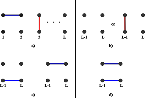
Figure 1: a) The numbering of columns in the strip. b) No dimers going across the last two columns. c) One dimer going across the last two columns. c) Two dimers going across the last two columns

We can motivate these recursion relations as follows: For the first relation, clearly, an additional vertical dimer can be added in the $x=L-1$ column in addition to not adding anything. For the second relation, two horizontal dimers can go across in the case of $Z_{1}(L)$ and one horizontal dimer in the case of $Z_{2}(L-1)$. For the third relation, the only scenario possible is two horizontal dimers going across for the case $Z_{1}(L-1)$. The corresponding matrix equation is:

$$\begin{bmatrix}Z_{1}(L)\\ Z_{2}(L)\\ Z_{3}(L)\end{bmatrix} =\begin{pmatrix}1+z&1&1\\ 2z&z&0\\ z^{2}&0&0\end{pmatrix}\begin{bmatrix}Z_{1}(L-1)\\ Z_{2}(L-1)\\ Z_{3}(L-1)\end{bmatrix}$$ (17)

which, using ideas from Sec. II.1, becomes:

$$\begin{bmatrix}Z_{1}(L)\\ Z_{2}(L)\\ Z_{3}(L)\end{bmatrix} =\begin{pmatrix}1+z&1&1\\ 2z&z&0\\ z^{2}&0&0\end{pmatrix}^{L-1}\begin{bmatrix}Z_{1}(2)\\ Z_{2}(2)\\ Z_{3}(2)\end{bmatrix}$$ (18)

Clearly, $\Omega_{L}(z)=Z_{1}(L+1)$ and $Z_{1}(2)=1+z$, $Z_{2}(2)=2z$, $Z_{3}(2)=z^{2}$ . Using the same spectral decomposition ideas as seen previously, we arrive at:

$$\Omega(L,z)=c_{1}\lambda_{1}(z)^{L}+c_{2}\lambda_{2}(z)^{L}+c_{3}\lambda_{3}(z)^{L}$$ (19)

While the cubic equation can be solved exactly in closed form, the expressions for the roots are rather complicated, and omitted here, which also does not allow us to do the same analysis as in Eq. (9). It is quite straightforward to calculate powers of $T$ directly by direct multiplication. We wrote a Mathematica code that evaluates the polynomials $Z_{i}(L)$ explicitly, and the determined the zeroes numerically for $L$ up to 200. The relation was explicitly checked by drawing configurations for $L=2,3,4$ and the notes and the corresponding codes on this have been uploaded on GitHub (see Acknowledgements for the link)

II.3 Results of code: Zeroes of the partition function

As mentioned in the last section, for the $2\times L$ strip, it is much easier to work with the Transfer matrix than the analytic expressions of the eigenvalues. The code for an input $L$, outputs the form of the partition function and its zeroes and plots them in the complex plane.

The results are what was expected: for any $L$, the zeroes lie on the negative real axis, while the density of zeroes approaches higher and higher values at one point, i.e., all the zeroes seem to congregate at that point. The plots are given in Fig. 2 for $L=25,40,\text{ and }100$. This is in perfect agreement with the theorem by Heilmann and Lieb applicable for any graph[9], which says that the zeroes of the partitions function of dimers on graphs always lie on the negative real axis. Our data is consistent with this result. From the graphs, We can ascertain that the critical point for the strips is $z_{0}\approx-0.251$ up to three decimal places numerically, which is in excellent agreement with the theoretical result. It is easy to see that near $z_{0}$, the eigenvalues $\lambda_{1}$ and $\lambda_{2}$ have a square root singularity.

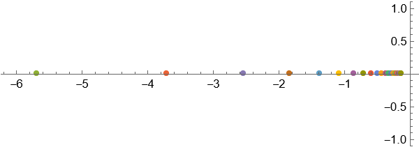
(a) L=25

(b) L=50

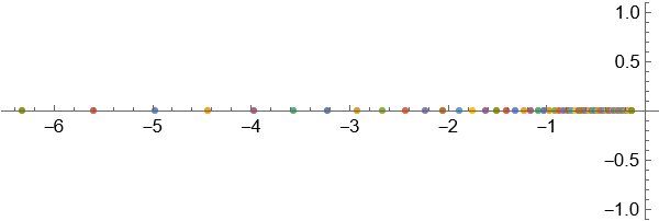
(c) L=100

Figure 2: Plots of zeroes of the partition function for varying L

III Trimers on $3\times L$ strip

Let us now look at the $k=3$ version of the problem. One immediate challenge that we face is the increased number of configurations to consider. However, utilizing symmetry arguments, we can make the problem much easier to deal with. There are primarily two notations that can be utilized in the transfer matrix method. The first is the standard notation commonly used in Statistical Mechanics to study lattice problems, while the second is something we found convenient while thinking about the problem.

III.1 Transfer Matrix method revisited

The setup is as follows: The strips go from left to right (the column numbering from 1 to L is from left to right), with each column having 3 sites. A trimer can occupy three sites on a line, and no two trimers can occupy the same site. Then we have the following two notations which can be used to establish the transfer matrix recursion relations:

• The configuration is denoted as $Z_{L}(h_{1},h_{2},h_{3})$, where $h_{i}\in\{0,1,2\}$. The $h_{i}$ denote how many sites to the right of the site at column $L$ and row $i$ are occupied by horizontal trimers(if 0, it means no sites to the right are occupied, if 1, it means that the horizontal trimer occupies that site, one site to the right and one to the left of row $i$ and column $L$, and 2 means that the site is a tail-end of a horizontal trimer extending to the right from the site on column $L$ and row $i$). We can see that the values $h_{1},h_{2},h_{3}$ defines the "rightmost boundary" of the total configuration. Vertical trimers are directly multiplied in these configurations (with a factor of $z$ as and when required)

• The configuration weights are denoted as $Z_{i}(L)$, $i\in\{1,2,3,4\}$, where: (i)i=1 means no horizontal trimer crosses from column number $x=L-2$ to $x=L$.(ii)i=2 means only one horizontal trimer crosses over from $x=L-2$ to $x=L$. (iii) i = 3 means two horizontal trimers cross over from $x=L-2$ to $x=L$, and i = 4 means three trimers cross over.

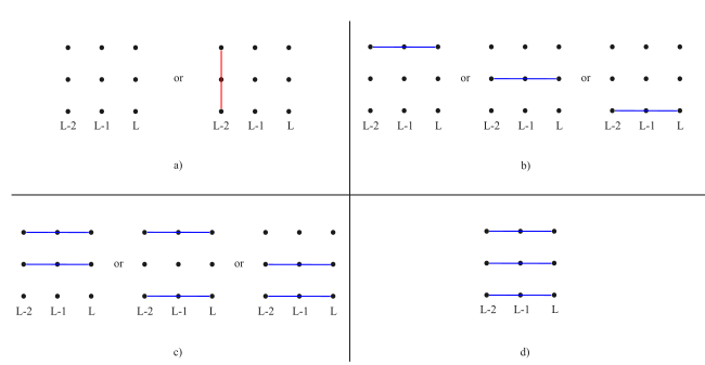
Figure 3: Pictorial representation of the second notation for partition functions of trimers on $3\times L$ strip. a) No trimer going across columns $L-2$ to $L$. b) One trimer going across columns $L-2$ to $L$. c) Two trimers going across columns $L-2$ to $L$. d) Three trimer going across columns $L-2$ to $L$.

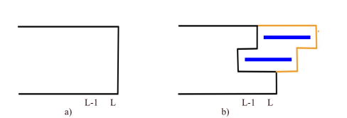
Figure 4: Examples of the first notation for partition functions of trimers on $3\times L$ strip. The orange dotted lines represent the extended boundary, while the black dotted lines represent the actual boundary a) $Z_{L}(0,0,0)$ b) $Z_{L}(2,1,0)$

Fig. 3 and Fig. 4 highlights these configurations in a pictorial manner. The first notation can be generalized to the general $k$-mers of $k\times L$ strip as configurations of the type $Z_{L}(h_{1},h_{2},h_{3}....h_{k})$, with $h_{i}\in\{0,1,2,...k-1\}$. A general lemma can be stated here about such configurations:

Lemma 1.

Let $S$ be the boundary of the strip configuration ( arrangement of $\{h_{i}\}$, $1\leq i\leq k$), such that at least one value is non-zero, i.e. $\exists i,h_{i}\neq 0$. Let $Z_{L}(S)$ be the configuration weight associated with $S$. Let $S^{\prime}$ be a permutation of $S$, such that $S^{\prime}=\{h_{i}^{\prime}\}$. Then $Z_{L}(S)$ = $Z_{L}(S^{\prime})$.

Sketch of Proof.

Since at least one $h_{i}\neq 0$, that implies that there cannot be any configuration with a vertical trimer on column $L$. This means that all configurations in $Z_{L}(S)$ have sites on column $L$ that can only be occupied by horizontal trimers, which satisfies the boundary conditions. But since, w.r.t the horizontal trimers, the boundary is symmetric, any permutation of $S$ (i.e. $S^{\prime}$) also has the same total configuration weight $Z_{L}(S)$, implying that $Z_{L}(S)$ = $Z_{L}(S^{\prime})$ ∎

Lemma 1 implies that only the unique boundary configurations ($S$) are necessary to find the recursion relation. The problem is similar to filling $k$ options that add up to k (the $k$ options are values between 0 to k-1, which can be chosen with repetition). Using standard combinatorics, this evaluates to a possible $2k-1\choose k$ configurations for $S$, which is also the length of the column vector in the transfer matrix method. For both methods to be valid, the dimensions of the Transfer Matrices should be the same in both the cases, as they encode the same problem in different ways. For $k=3$, there are $3^{3}$ basic partition functions, but the size of the matrix can be reduced by using these symmetries of the problem. This evaluates to a $10\times 1$ vector on which a $10\times 10$ (reduced) matrix acts on. The details on how the transfer matrix is arrived at, and the transformation between the two methods is listed in Appendix A. We use the second notation to derive the transfer matrix recursion $X_{L+1}=\Gamma(z)X_{L}$, where we have:

$$\Gamma(z) =\begin{pmatrix}1+z&0&0&0&1&1&1&z^{2}+2z&z&2z^{2}\\ 3z&0&0&0&2z&z&0&4z^{2}&2z^{2}&0\\ 3z^{2}&0&0&0&z^{2}&0&0&2z^{3}&z^{3}&2z^{4}\\ z^{3}&0&0&0&0&0&0&0&0&0\\ 0&1&0&0&0&0&0&0&0&0\\ 0&0&1&0&0&0&0&0&0&0\\ 0&0&0&1&0&0&0&0&0&0\\ 0&0&0&0&1&0&0&0&0&0\\ 0&0&0&0&0&1&0&0&0&0\\ 0&0&0&0&0&0&0&1&0&0\\ \end{pmatrix}$$ (20)

$$X_{L} =[Z_{1}(L+1),Z_{2}(L+1),Z_{3}(L+1),Z_{4}(L+1),Z_{2}(L),$$

$$Z_{3}(L),Z_{4}(L),Z_{2}(L-1),Z_{3}(L-1),Z_{2}(L-2)]^{T}$$

III.2 Results and plots of the codes

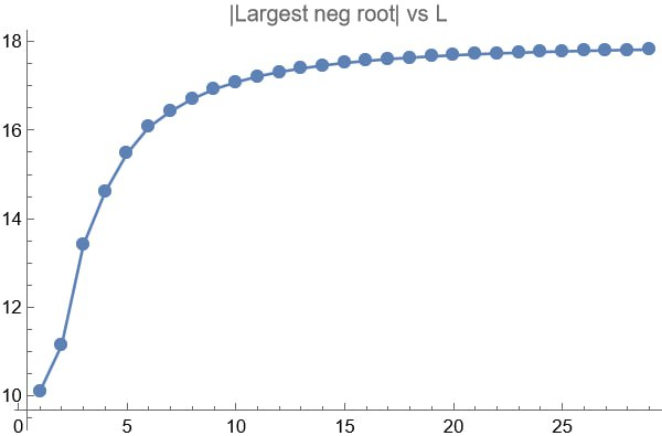
Figure 5: Modulus of largest negative root v/s $L/6$, starting from $L=10$

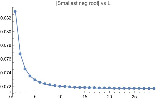
Figure 6: Modulus of smallest negative root v/s $L/6$, starting from $L=10$

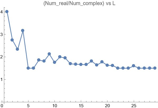
Figure 7: (ratio of real roots to complex roots v/s $L/6$, starting from $L=10$. The value asymptotically reaches 1.5 for large $L$

In this section, all the plots obtained via our Mathematica code are displayed. We consider all plots starting from $L\geq 10$ as otherwise the system size is too small to be of any significance. Since all roots $z$ are such that $\mathcal{R}e(z)<0$, we say that the smallest negative root is the one where $\mathcal{R}e(z)$ is closest to zero, and the largest negative root is the one where $Re(z)$ is the farthest from it. Fig. 5 and Fig. 6 plot the modulus of largest and smallest negative roots as a function of $L$, while Fig. 7 plot the ratio of real roots to imaginary ones as a function of L.

We observe that both the largest and smallest negative roots lie in the annulus $x\leq z\leq y$ , implying the fact that in the thermodynamic limit ($L\rightarrow\infty$), all roots of the partition function are bounded between two values $x$ and $y$, which are $x\approx-17.34$ (the actual largest negative root is imaginary and always comes n conjugate pairs, with values around $-17.34\pm i3.36$) and $y=-0.071$, such that for any $z$ to be a root of the partition function $\lim_{L\to\infty}\Omega(z,L)$, we have $x\leq Re(z)\leq y$. This result can be also seen analytically, if we consider the characteristic equation of the partition matrix $f(\lambda)=|T-\lambda I|=0$ (where $|A|$ means determinant of matrix A), then we have:

$$f(\lambda)= \lambda^{10}-\lambda^{9}(1+z)-\lambda^{8}(2z)-\lambda^{7}(z+5z^{2}+2z^{3})-$$

$$\lambda^{6}(2z^{2}+2z^{3}-z^{4})-\lambda^{5}(5z^{3}-z^{4})+\lambda^{4}(2z^{4}+z^{5}+z^{6})-$$

$$\lambda^{3}(10z^{5}+4z^{6})-\lambda^{2}(8z^{6}-6z^{7})+\lambda(2z^{8})+4z^{9}$$

The expression $f(\lambda)=0$ gives us the eigenvalues of the transfer matrix as a function of $z$. If we put $\lambda=zy$ and divide he entire expression by $z^{10}$ we have:

$$f(y)=0=y^{10}-y^{9}(1+\frac{1}{z})-y^{8}(\frac{2}{z})-y^{7}(2+\frac{5}{z}+\frac{1}{z^{2}})+...$$

This equation can be solved for $y$ as a function of $\frac{1}{z}$, and is well-behaved for large $z$. Thus we have that:

$$y(z) =y_{0}(1+\frac{A_{1}}{z}+\frac{A_{2}}{z}+...)$$ (21)

$$\lambda(z) =y_{0}z(1+\frac{A_{1}}{z}+\frac{A_{2}}{z}+...)$$ (22)

This thus implies that since $z\to\infty$ is not a singular point for the function $ln(\lambda/z)$, the zeroes are bounded in a finite region.

Clearly, if most of the density of zeroes is within a distance $R$ of the origin, then analogous to charges on a line, they produce an "electric field" $Q/z$ at $z>>R$, where Q is the "total charge density". For reference, the density of covered sites per total numer of sites is obtained from the partition function as:

$$\rho(z)=z\frac{dln\lambda}{dz}$$ (23)

where $\lambda$ is the largest eigenvalue of the transfer matrix. It is easily seen that if $\lambda=kz(1+A_{1}/z+A_{2}/z^{2}+...)$, then at $z\to\infty$, the density will be a constant (equal to $Q$, if we go by the general electric charge analogy where $\rho=z\partial V/\partial z$ with $V\equiv|ln\lambda|$ as the potential) . At large real positive but finite $z$, we can say that the density function takes the laurent expansion form of $\rho=A+B/z+C/z^{2}+\cdots$, which could be understood as:

$$\rho(z)=\rho_{\infty}-\frac{A}{z^{a}}+\text{ higher order corrections }$$ (24)

This form determines the behaviour of density at large real positive but finite $z$. We can also ask how much the density as a function of $z$ deviates from the thermodynamic limit in case of L being finite. Also note that since the real part of $ln(\lambda(z))$ is the electrostatic potential due to the charge distribution. Then one can calulate the electric field, and the discontinuity in the normal component of electric field gives the charge density on the line of zeroes. This is a way to directly determine it from $\lambda(z)$.

III.3 Ways of reducing dimension, and other possible approaches

Let us motivate how to reduce the dimensionality of the transfer matrix method(i.e. reduce the number of independent configurations required as follows).Instead of working with partition functions, we now work with generating functions. Take the generating function $f(x,h_{1},h_{2},h_{3})$ defined as:

$$f(x,h_{1},h_{2},h_{3})=\sum_{L=0}^{\infty}x^{L}\Omega_{L}(h_{1},h_{2},h_{3})$$ (25)

Take $h_{1}=2,h_{2}=2\text{ and }h_{3}=2$ as an example. Clearly, we see that $\Omega_{L}(2,2,2)$ can only give rise to $\Omega_{L+1}(1,1,1)$, which can only give rise to $\Omega_{L+2}(0,0,0)$. Essentially, this can be easily seen in the generating function, by just putting $f(0,0,0)=xf(1,1,1)=x^{2}f(2,2,2)$ (omitting $x$ inside the function argument as it is understood). Similarly, we can see that only those values of ($h_{1},h_{2},h_{3}$) are required where $h_{i}\geq 1$. This gives us that the independent triad(s) are $(h_{1},h_{2},h_{3})=\{(0,0,0),(0,0,1),(0,1,1),(0,1,2),(0,0,2),(0,2,2)\}$ reducing the dimensionality from 10 to 6. This method also works for a general $k$-mer on a $k\times L$ strip. Essentially, the argument becomes that only the triad(s) where there is at least one value equal to 0 forms the independent basis. Thus, using these, we can form a transfer matrix formulation in the generating function formalism:

$$MF=X$$ (26)

$$F=M^{-1}X$$ (27)

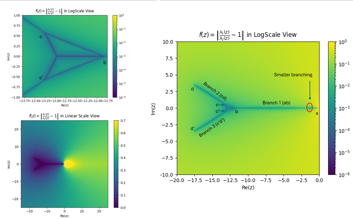
Figure 8: Heatmap images of the absolute ratio distance from 1. Image on the right highlights the eight (possibly curved) segments of zeroes with the important endpoints ($a=-0.0071,b=-11.82,c=-13.25+i0.25,d=-17.47+i3.41$, $c^{\prime},d^{\prime}$ are complex conjugates of points $c$ and $d$ respectively). Top left heatmap gives a closer look on the branching starting from point $b$, while bottom left image is a zoomed out linear scale view of the same scenario.

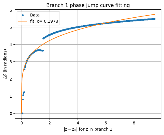
(a) Branch 1 curve fit

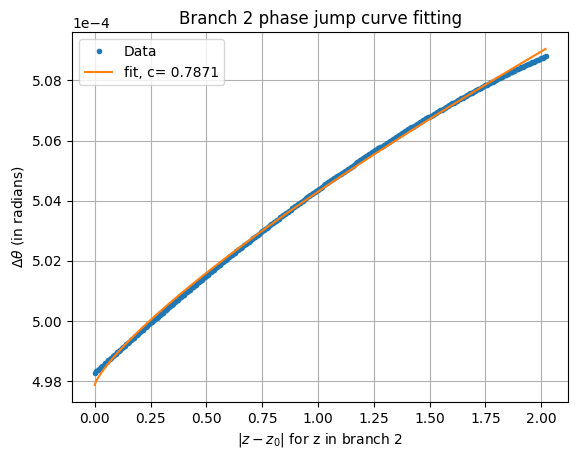
(b) Branch 2 curve fit

Figure 9: Phase jump plots for Branch 1 and Branch 2 along with their respective curve fits for the proportional integrated density of zeroes curve. Notice that the sudden discontinuity for branch 1 just before $|z-z_{0}|=2$ is due to the smaller branching (red oval in Fig. 8) in the line of zeroes. Also notice that in branch 2, the phase jump is of the order of magnitude of $10^{-4}$. It was checked in the code that while this line segment of zeroes is present in the heatmap, on these points the absolute ratio of eigenvalues is not robustly close to 1, and seems to be present only upto a tolerance level of $10^{-6}$, while branch 1, the line of zeroes persist upto a tolerance level of $10^{-15}$, which can be reasonably attested to numerical error margins.

where $F$ is the column vector of generating functions, and $X$ is a constant vector.

We have also seen that our current transfer matrix method does not work very well for large $L$ ($L\approx 1000$ seems to be the current maximum if the system is allowed to run for 1 day). Numerical errors also creep in at higher values of $L$ which are difficult to control. Another method, which can be much faster, is listed: Consider the partition function $\Omega_{L}(z)$, and let $\{\lambda_{i}(z)\},1\leq i\leq 10$ , such that $|\lambda_{i}(z)|>|\lambda_{j}(z)|$ for $i>j$. It is easily seen that $\Omega_{L}(z)=\sum_{i}\lambda_{i}(z)^{L}$ (normalised such that any coefficients $c_{i}$ are absorbed into the eigenvalues). Let us only consider the first two largest eigenvalues, such that:

$$\tilde{\Omega}_{L}(z)=\lambda_{1}(z)^{L}+\lambda_{2}(z)^{L}$$ (28)

For large $L$, this function is a very close approximation to the actual partition function. Hence, we can just equivalently find roots of $\tilde{\Omega}_{L}(z)$, which will just give:

$$\left(\frac{\lambda_{1}(z)}{\lambda_{2}(z)}\right)^{L}=-1$$ (29)

$$\frac{\lambda_{1}(z)}{\lambda_{2}(z)}= e^{i\theta},\text{ where }\theta=\frac{(2m+1)\pi}{L}$$ (30)

Numerically, it is easy to determine the phase (values of $\theta$) in the complex z-plane where $\frac{|\lambda_{1}(z)|}{|\lambda_{2}(z)|}=1$. We just take any starting point $z_{0}$ and move in the direction which decreases (or increases, depending on the initial value) the value of $\frac{|\lambda_{1}(z)|}{|\lambda_{2}(z)|}$ the fastest. Once we reach a value of $z$ where the ratio is $\approx 1$ to an agreed accuracy, we find other such values of $z$ by moving in a direction where this condition is maintained. Once we have the line where the zeroes will be in the large $L$ limit, as we move along the line, the density of zeroes depend on how the value of $\theta$ fluctuates, which gives us essentially the integrated density of zeroes. We analyze the jump in phase for $ln(\lambda_{max}(z))$ across the branch cuts defined by the zeroes of the partition function and relate it to the integrated density of zeroes (see Appendix B for details)

The results complement the finite $L$ numerics. Fig. 8, highlights the heatmap images of this algorithm, where the colorbar indicates the absolute distance of the ratio from 1. Fig. 9 highlights the phase jump plots on two of the three main branches (as branch 2 and 3 are complex conjugate, they have the same phase jump plots) considered on the heatmap, as a function of the increasing distance from singularity considered for the branch. We find that the curves are of the form $f(z)=a|z-z_{0}|^{c}$, $c_{num}=0.198$ for branch 1, while $c_{num}=0.787$ for branch 2. Note that for branch 1, point $a$ is quivalent to $z_{0}$, while for branch 2, it is point $d$ (see Fig. 8 right figure). We see that while branch 1 has a considerable phase jump, the same is not true for branch 2 where the phase jump is of the order of $10^{-4}$. The curve fits have been done close to the singularity points for better accuracy.

IV Discussion and Outlook

We summarise our findings in the following section:

1. We firstly checked our transfer matrix recursion methods for a few cases of dimers $k=2$ on 1D-line and $2\times L$ strip. We found that the partition function zeroes were all on the negative real axis, going from $z_{0}=-0.25$ upto $-\infty$ as theoretically proved in [9].

2. On extending the study to trimers on $3\times L$ strips, we made use of certain symmetries to reduce our transfer matrix dimensions, and surprisingly found that the obtained zeroes are bounded in the complex plane (as highlighted in Fig. 8), as opposed to the dimer case, where the zeroes are unbounded. The presence of imaginary zeroes in not so surprising, as it can be seen in trivial configurations involving trimers on finite sized $3\times L$ strips.

3. Our current transfer matrix formalism may very easily be extended to higher $k$’s, which can be utilised to generally study $k$-mers on a 2D lattice. One interesting problem can be to numerically study trimers on a general $k\times L$ structure, for which there are no known theoretical results to the best of the authors’ knowledge.

Appendix A Derivation of the transfer matrix

Here we will essentially sketch the derivation of the transfer matrix utilizing the first formulation. The key point to notice that all $Z_{i}(y)$ for $y\leq L-3$ is essentially all covered amongst the configurations of $L-2\leq y\leq L+1$ in $X_{L}$ (see Eq. (LABEL:eqn:tm_main)). To see this, we show in Fig. 10 the two contribution from the lowest strip length configuration which is $Z_{2}(L-2)$ for $Z_{1}(L+2)$ giving the $2z^{2}Z_{2}(L-2)$ term:

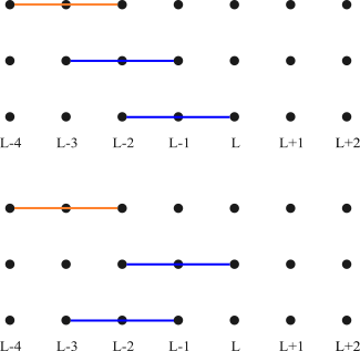
Figure 10: Contribution to $Z_{1}(L+2)$ from $Z_{2}(L-2)$ (orange) and two horizontal trimers (blue) giving the $z^{2}$ term in the product. Since for each $Z_{2}(L-2)$ configuration, there are two ways of placing the two trimers, hence the term $2z^{2}Z_{2}(L-2)$.

No other $L-2$ term exists, and also no lower strip length term ($y<L-2$) is required in the recursion, as they have already been covered in the $L+1$ length terms. All the other terms of the recursion are also formed in the same fashion. $Z_{1}(y)$ for $y<L+1$ is covered under $Z_{1}(L+1)$. Similarly $Z_{4}(y)$ for $y<L$ is also covered under $Z_{1}(L+1)$, while $Z_{3}(L-2)$ is covered by $Z_{2}(L),Z_{2}(L-1)$ and $Z_{1}(L+1)$.

The transformation from the first notation to the second one is also easily understood with pictorial representations. The key idea is that sum of configurations with permutation of some values of $h_{1},h_{2},h_{3}$ essentially equals some sum of configurations in the first notation. We trivially note down that $Z_{1}(L+2)=Z_{L}(0,0,0)$,$Z_{4}(L+1)=Z_{L}(1,1,1)$ and $Z_{2}(L+1)=Z_{L-1}(2,0,0)+Z_{L-1}(0,2,0)+Z_{L-1}(0,0,2)$. We know look at $h_{1}=0,h_{2}=0,h_{3}=1$ and its permutations, and see its sum, i.e. $Z_{L}(0,0,1)+Z_{L}(0,1,0)+Z_{L}(1,0,0)=3Z_{L}(0,0,1)$ in Fig. 11. Essentially, we see that:

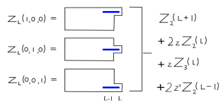
Figure 11: An example for showing transformation from first notation to the second notation, described in Sec. III.1.

$$3Z_{L}(0,0,1)=Z_{2}(L+1)+2zZ_{2}(L)+zZ_{3}(L)+2z^{2}(L-1)$$ (31)

The R.H.S contains all the configurations in the first notation which satisfy the boundary conditions of the L.H.S in the second condition. We can similarly do the same for all the independent configurations of the partition function in the second notation, and arrive at the equation $\tilde{X}_{L}=U(z)X_{L+1}$, where:

$$U(z)=\begin{pmatrix}1&0&0&0&0&0&0&0&0&0\\ 0&0&0&0&1/3&0&0&2z/3&z/3&2z^{2}/3\\ 0&0&0&0&0&1/3&0&z^{2}/3&0&0\\ 0&0&0&0&0&0&1&0&0&0\\ 0&1/3&0&0&0&0&0&0&0&0\\ 0&0&1/3&0&0&0&0&0&0&0\\ 0&0&0&1/3&0&0&0&0&0&0\\ 0&0&0&0&z/3&0&0&z^{2}/3&0&0\\ 0&0&0&0&0&z^{2}/3&0&0&0&0\\ 0&0&0&0&z/3&0&0&0&0&0\\ \end{pmatrix}$$ (32)

$$\tilde{X}_{L}=[Z_{L}(0,0,0),Z_{L}(0,0,1),Z_{L}(0,1,1),Z_{L}(1,1,1),$$

$$Z_{L}(0,0,2),Z_{L}(0,2,2),Z_{L}(2,2,2),Z_{L}(0,1,2),Z_{L}(1,2,2),$$

$$Z_{L}(1,1,2)]^{T}$$

Appendix B Branch cuts for the phase jump plotting

Here we discuss the relation between the density of zeroes per unit length, which is $\lim_{L\to\infty}\phi_{L}/L$, where $\phi_{L}$ is the density of zeroes on a branch. We define $\phi_{L}^{i}(z)$ to be the density corresponding to branch $i=1,2,3$ as according to Fig. 8. Note that this density is different from $\rho(z)$ which is density of filled sites per total number of sites in the lattice as a function of activity. We note the following expressions:

$$\rho(z)=\frac{z}{L}\frac{\partial ln(\Omega_{L}(z))}{\partial z}$$ (33)

where $\Omega_{L}(z)$ is the partition function for a finite strip of length $L$. We can write $\Omega_{L}(z)\approx\lambda_{max}^{L}(z)$, where $\lambda_{max}$ is the eigenvalue of the transfer matrix with the highest magnitude at $z$, and thus have:

Define $\theta$ as the phase of the complex-valued function $ln(\lambda_{max}(z-z_{0}))$, where $z_{0}$ is the endpoint of a branch cut, thus making it dependent on $z$ itself. Since the natural log function is multivalued in the complex plane, we carefully choose the direction of our branch cuts (originating from the zeroes of the partition function) such that the cuts overlap on the direction of the line of zeroes and thus cancel out outside of ki0these lines. Fig. 13 highlights these branch cuts. These endpoints $z_{0}$ are chosen carefully such that when a contour integral is performed as in Fig. 13, the encompassed zeroes are proportional to the phase jump across the branch cut discontinuity. We formally note that if $\Omega_{L}(z)=|\Omega_{L}(z)|e^{i\theta}$:

$$\frac{ln(\Omega_{L}(z))}{L}=\frac{ln(|\Omega_{L}(z)|)}{L}+i\frac{\theta}{L}$$ (34)

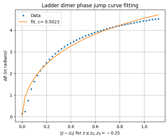
Figure 12: Phase jump plot with curve fitting of the configuration in Sec. II.2. The fit value is for the integrated density of zeroes curve

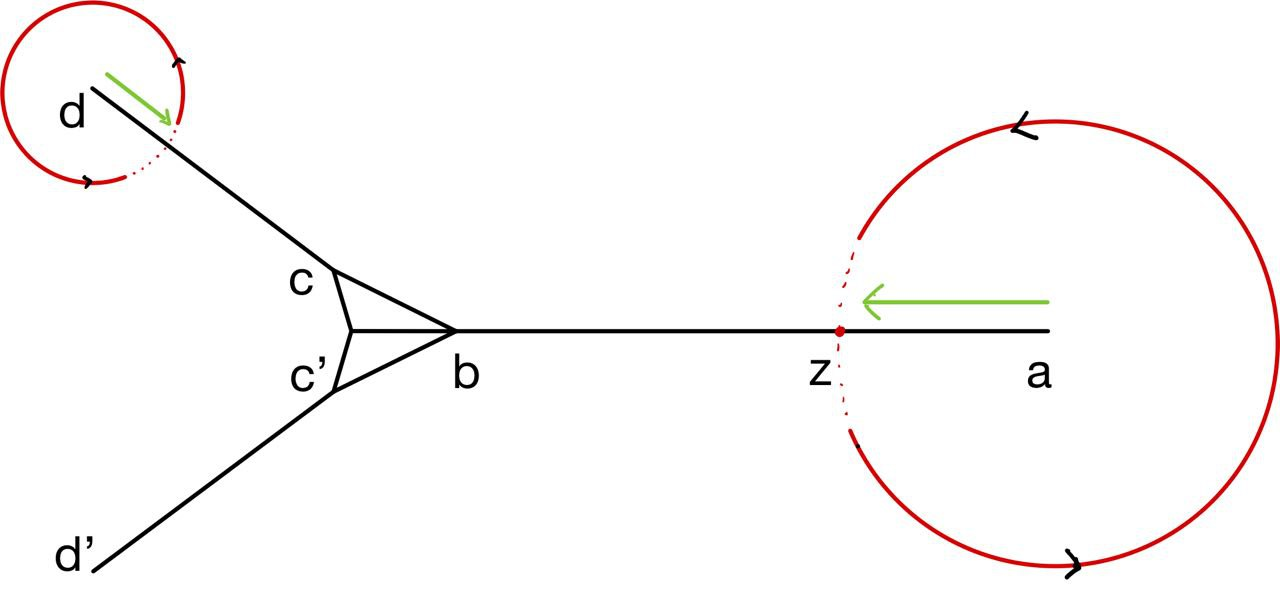
Figure 13: Branch cuts with examples of contour lines. In this scenario, points $a$ and $d$ are the singularity points ($z_{0}$) for branches 1 and 2, respectively. The green lines highlight the zeroes encompassed by the contour lines (drawn in red)

Here, the $\theta/L$ term is multivalued as $\theta\to\theta+2\pi n$ is also a valid phase. If we take each zero to have an analogous charge of $1/L$, crossing the branch cut starting from one such "charge" will give a phase jump of $2\pi/L$. Similarly, if the contour crosses the common branch cut from two charges, the phase jump will be $4\pi/L$. Generalizing this, the phase jump ($\Delta\theta$) is equal to $2\pi n/L$, where $n$ is the number of encompassed zeroes. But note that in the thermodynamic limit, $\lim_{L\to\infty}n/L=\int_{z_{0}}^{z}\phi(t)dt$, where $z$ is the point encompassing the $n$ zeroes.

$$2\pi\int_{z_{0}}^{z}\phi(t)dt =\Delta\theta$$ (35)

$$\int_{z_{0}}^{z}\phi(t)dt =\frac{\Delta\theta}{2\pi}$$

We can extract the power-law expressions of the density of zeroes of the form of $|z-z_{0}|^{c}$ close to the singularity $z_{0}$ (as expressed in the original Lee-Yang paper), the integrated density of zeroes will be of the form of $|z-z_{0}|^{c+1}$. We can find the value of $c$ by curve-fitting power law expressions to our phase jump plots. As a test of accuracy for this method, Fig. 12 shows the curve fitting to the phase jump plot on the dimer on ladder problem (refer Sec. II.2), for which it is known that $c=-0.5$. With our curve fit of the form $f(x)=ax^{c}$, we obtained $c_{num}=0.5023$, giving the power law exponent as equal to $-0.4977$, which is reasonably close to the correct theoretical value. The code essentially calculates this phase jump above and below the branch cuts (after correctly formulating the phase range), and we plot this phase jump as a function of distance from singularity, or $|z-z_{0}|$.

References

- Yang and Lee [1952] C. N. Yang and T. D. Lee, Statistical theory of equations of state and phase transitions. i. theory of condensation, Phys. Rev. 87, 404 (1952).
- Lee and Yang [1952] T. D. Lee and C. N. Yang, Statistical theory of equations of state and phase transitions. ii. lattice gas and ising model, Phys. Rev. 87, 410 (1952).
- Fisher [1965] M. E. Fisher, The nature of critical points, Lectures in Theoretical Physics 7C, 1 (1965).
- [4] R. J. Baxter, Exactly solved models in statistical mechanics, in Integrable Systems in Statistical Mechanics, pp. 5–63.
- Temperley and Lieb [1971] H. N. V. Temperley and E. H. Lieb, Relations between the ‘percolation’ and ‘colouring’ problem and other graph-theoretical problems associated with regular planar lattices: Some exact results for the ‘percolation’ problem, Proceedings of the Royal Society of London. Series A, Mathematical and Physical Sciences 322, 251 (1971).
- Fraden et al. [1989] S. Fraden, G. Maret, D. L. D. Caspar, and R. B. Meyer, Isotropic-nematic phase transition and angular correlations in isotropic suspensions of tobacco mosaic virus, Phys. Rev. Lett. 63, 2068 (1989).
- Gennes and Prost [2023] P. Gennes and J. Prost, The Physics of Liquid Crystals (2023).
- Islam et al. [2004] M. F. Islam, A. M. Alsayed, Z. Dogic, J. Zhang, T. C. Lubensky, and A. G. Yodh, Nematic nanotube gels, Phys. Rev. Lett. 92, 088303 (2004).
- Heilmann and Lieb [1972] O. J. Heilmann and E. H. Lieb, Theory of monomer-dimer systems, Communications in Mathematical Physics 25, 190–232 (1972).