S-MolSearch: 3D Semi-supervised Contrastive Learning for Bioactive Molecule Search

Abstract

Virtual Screening is an essential technique in the early phases of drug discovery, aimed at identifying promising drug candidates from vast molecular libraries. Recently, ligand-based virtual screening has garnered significant attention due to its efficacy in conducting extensive database screenings without relying on specific protein-binding site information. Obtaining binding affinity data for complexes is highly expensive, resulting in a limited amount of available data that covers a relatively small chemical space. Moreover, these datasets contain a significant amount of inconsistent noise. It is challenging to identify an inductive bias that consistently maintains the integrity of molecular activity during data augmentation. To tackle these challenges, we propose S-MolSearch, the first framework to our knowledge, that leverages molecular 3D information and affinity information in semi-supervised contrastive learning for ligand-based virtual screening. Drawing on the principles of inverse optimal transport, S-MolSearch efficiently processes both labeled and unlabeled data, training molecular structural encoders while generating soft labels for the unlabeled data. This design allows S-MolSearch to adaptively utilize unlabeled data within the learning process. Empirically, S-MolSearch demonstrates superior performance on widely-used benchmarks LIT-PCBA and DUD-E. It surpasses both structure-based and ligand-based virtual screening methods for enrichment factors across 0.5%, 1% and 5%.

1 Introduction

Virtual Screening [1, 2, 3, 4] plays a crucial role in the early stages of drug discovery by identifying potential drug candidates from large molecular libraries. Structure-Based Virtual Screening (SBVS) [5, 6, 7, 8], a widely used virtual screening method, attempts to predict the best interaction between ligands against a protein target to form a protein-ligand complex. Recently, deep learning methods have also been explored. Methods trained on affinity labels  [9, 10, 11] conduct virtual screening by modeling binding affinities and ranking based on prediction. Additionally, a method [12] uses similarities between embedding of pockets and molecules to search for active molecules. However, these SBVS methods cannot escape the dependency on the structure of protein targets, which is unavailable for challenging or novel targets, such as disordered proteins like c-Myc, limiting the applicability of SBVS. Besides, plenty of assays used in Virtual Screening [13] are cell-based rather than target-specific, introducing noise into the active molecules since their activity is not entirely dependent on interaction with the protein target.

To remedy this, Ligand-Based Virtual Screening (LBVS) [14, 15, 16, 17, 18] searches similar molecules via known bioactive molecules and does not depend on the structure of protein targets, which has attracted increasing attention. Computational LBVS methods [19, 20, 18] rigidly employ structural similarity to search for molecules, often using atom-centered, smooth Gaussian overlays to assess molecular similarity. Searching for bioactive molecules needs to consider both structure and electronic similarity. Some methods [14] also require charge comparison, which is expensive and time-consuming. These methods struggle with inefficiency when handling large databases. Moreover, since only structural or charge information is considered while affinity is ignored, even if molecules with similar structures or charges are identified, they may still exhibit poor affinity in practical applications due to activity cliffs [21].

A natural question arises: how can we enhance LBVS by collecting molecule similarity data from large-scale unlabeled molecules? To search both similar and bioactive molecules, we can choose those bioactive molecules that bind to the same protein. Meanwhile, labeled molecule-protein binding data is limited due to the expensive affinity acquisition. Also various standards [22, 13] across different datasets, introducing substantial noise. It is difficult to cover the searching chemical space with affinity data alone. A feasible solution is to leverage similarity from finite affinity data to broader chemical space.

Inspired by the success of contrastive learning [23, 24, 25, 26], which can extract informative representations from large-scale data, we explore its feasibility for molecule data. However, those data augmentation techniques in vision or language cannot be directly applied to molecules due to their inherent 3D structure. This limitation stems from a lack of inductive bias to guarantee augmentation maintains the integrity of molecular activity.

To address the challenges, we propose S-MolSearch, a novel semi-supervised contrastive learning framework based on inverse optimal transport (IOT) [27]. S-MolSearch directly uses 3D molecular structures to capture structure similarity. It consists of two main components: one encoder $f_{\theta}$ for labeled dataset and another encoder $g_{\psi}$ for the full dataset, which includes both labeled and unlabeled data. Both encoders are trained simultaneously to effectively leverage the two types of data. We organize a dataset of labeled molecule-protein binding data from ChEMBL [28]. Molecules are assigned to different targets based on binding affinity, with the active molecules corresponding to each target forming clusters. We sample from these clusters, treating molecules from the same cluster as positive samples and those from different clusters as negative samples to train encoder $f_{\theta}$. This approach incorporates affinity information into training and avoids the limitation caused by relying solely on structural similarity. For the update of encoder $g_{\psi}$, we assume that the similarity measurements obtained by encoder $f_{\theta}$ can be generalized to unlabeled data. We input the same data from the full dataset into these two encoders separately and use optimal transport to obtain soft labels from $f_{\theta}$. The encoder $g_{\psi}$ is then trained using these soft labels. This integration enables S-MolSearch to effectively utilize unlabeled data, ensuring that the model learns from both affinity-labeled samples and broader structural similarities across the molecular dataset.

Empirically, S-MolSearch demonstrates superior performance on widely-used benchmarks LIT-PCBA [13] and DUD-E [22]. It consistently achieves state-of-the-art results, surpassing both SBVS methods and LBVS methods for enrichment factors across 0.5% 1% and 5%. Notably, S-MolSearch trained on data filtered with a sequence similarity of 0.9 exceeds the best baseline by more than 30% on DUD-E. These results provide strong empirical support for the effectiveness of S-MolSearch, confirming its advanced capability for virtual screening.

Our main contributions are summarized as follows:

• We introduce S-MolSearch, which is the first time integrates both molecular 3D structures and affinity information into molecule search.

• Built upon inverse optimal transport, we develop a semi-supervised contrastive learning framework, which induces S-MolSearch. By combining limited labeled data with extensive unlabeled data, S-MolSearch can learn more informative representations and explore the chemical space more effectively.

• S-MolSearch is evaluated on widely-used benchmarks LIT-PCBA and DUD-E, surpassing both SBVS and LBVS methods to achieve state-of-the-art results.

2 Related work

2.1 Virtual Screening

Virtual screening can be broadly divided into two main categories: Structure-Based Virtual Screening (SBVS) and Ligand-Based Virtual Screening (LBVS). SBVS [5, 6, 7, 8] heavily relies on the structure of protein targets and typically employs molecular docking. Recently, many deep learning methods [29, 10, 11, 12] have also emerged. In contrast, LBVS [14, 15, 16, 17, 18] uses known active ligands as seeds to identify potential ligands. Molecule search is a major LBVS approach, typically divided into two categories: 2D similarity search and 3D similarity search. 2D molecule search methods [30, 31] use molecular fingerprints to search for similar molecules, while 3D molecular search methods [15, 16, 18] depend on shape overlap.

2.2 Optimal Transport and inverse optimal transport

Optimal Transport (OT) is a mathematical problem that aims to determine the most efficient way to redistribute one initial distribution (known as the source distribution) into another distribution (known as the target distribution) while minimizing a defined transportation cost. To handle computational complexities, OT often incorporates regularization [32], leading to a softened optimization problem. The regularized OT objective is a convex function, thereby ensuring a unique solution that can be efficiently solved using iterative methods [33, 34].

Inverse Optimal Transport (IOT) seeks to determine the cost matrix that explains an observed optimal transport.  [27] introduces a method to infer unknown costs.  [35] explores the mathematical theory behind IOT. In many IOT studies [36, 37], optimization is directly performed over the cost matrix, typically focusing on learnable distances between samples rather than on the sample features.

2.3 Semi-supervised learning

Semi-supervised learning [38, 39, 40, 41] is typically used in scenarios where labeled data is limited but unlabeled data is abundant. Pseudo-labeling [42] is a classic technique of semi-supervised learning. [43] introduce a self-ensembling method that generates pseudo-labels by forming a consensus prediction using the outputs of the network under different regularization and augmentation conditions. UPS [44] proposes an uncertainty-aware pseudo-label selection framework that improves pseudo-labeling accuracy by reducing the amount of noise in the training process. UST [45] employs a teacher-student training paradigm. The teacher model is responsible for selecting and generating pseudo-labels, while the student model learns from the labeled set augmented with these pseudo-labels. Recent work [46] utilizes additional unpaired images to construct caption-level and keyword-level pseudo-labels, enhancing training.

3 Method

3.1 Overview

Molecular similarity search is a type of ligand-based virtual screening whose purpose is to perform a rapid search and filtering of similar molecules in a molecular database based on a query molecule provided by the user. We model the task as a dense retrieval problem, using a well-trained encoder to extract embedding representations of molecules and rank them by their cosine similarity to a query molecule, thereby identifying the top $k$ most similar candidates.

Building upon the principles of inverse optimal transport (IOT), we have developed the S-Molsearch method. As shown in Figure 1, S-Molsearch uses a molecular structure encoder $f_{\theta}$ for labeled dataset $D_{sup}$ and another encoder $g_{\psi}$ for the full dataset $D_{full}$, encompassing both labeled and unlabeled dataset. $f_{\theta}$ utilizes contrastive learning to learn from labeled dataset. $g_{\psi}$ optimizes its parameters using the soft labels produced by $f_{\theta}$, which have been processed through smooth optimal transport. The two encoders are initialized with a molecular pretraining backbone Uni-Mol [47]. Both encoders are trained simultaneously under the guidance of a unified loss function $\mathcal{L}_{total}$. The encoder $g_{\psi}$, trained on full dataset, is used for inference.

Figure 1: Overview of S-MolSearch Framework

In the following sections, we will provide more details about the core components and training strategies that underpin S-Molsearch. In section 3.2, we explain the pretraining backbone of the molecular structural encoder, Uni-Mol. In sections 3.3 and 3.4, we will sequentially examine the training strategies for both $f_{\theta}$ and $g_{\psi}$. In section 3.5, we will discuss the regularization techniques employed to enhance model generalizability and stability. In section 3.6, we will provide an analysis of S-Molsearch from the perspective of IOT, offering insights into its methodological strengths.

3.2 Pretraining Backbone of Molecular Encoder

To effectively encode the structural information of molecules, we choose Uni-Mol as the backbone of molecular encoder for S-Molsearch. Uni-Mol is a molecular pretraining model specifically designed to adeptly process molecular 3D conformation data. It has achieved state-of-the-art performance across a range of downstream tasks. The UniMol model utilizes a self-attention mechanism that incorporates distance bias to integrate information about atoms and their spatial relationships, thereby generating a structural representation of molecules. The molecular embedding is created by using the embedding of the CLS token, and the embedding vector is normalized using the Euclidean norm.

3.3 Training Strategy of Encoder on Labeled Dataset

In this part, we employ molecular-protein binding data sourced from the ChEMBL. Molecules are assigned to different targets based on binding affinity. The active molecules corresponding to each target form clusters. We sample from these clusters to obtain data for contrastive learning. Molecules from the same cluster are considered positive pairs, while molecules from different clusters are considered negative pairs. We employ InfoNCE loss for encoder $f_{\theta}$ on labeled dataset, as shown in Equation 1:

$$\mathcal{L}_{sup}=-\sum_{i=1}^{N}\log\frac{\exp(\text{sim}(x_{i},y_{i})/\tau)}{\sum_{j=1}^{N}\exp(\text{sim}(x_{i},y_{j})/\tau)}$$ (1)

Where $x_{i}$ and $y_{i}$ are the embeddings of positive molecule pairs, and $x_{i}$ and $y_{j}$ form negative molecule embedding pairs within the batch when $j\neq i$, $\text{sim}(x,y)$ denotes the similarity score between embeddings, typically computed as the inner product of the normalized vectors $xy^{T}$, $\tau$ is the temperature parameter that scales the similarity scores. By utilizing the InfoNCE loss, $f_{\theta}$ pulls the embeddings of positive samples close while enforcing them away from the negative samples in the embedding space.

3.4 Training Strategy of Encoder on Full Dataset

To harness large-scale unsupervised data effectively, S-MolSearch utilizes the $f_{\theta}$ to guide the learning of another encoder on full data $g_{\psi}$. Specifically, we employ $f_{\theta}$ to preprocess the data for the $g_{\psi}$, ensuring that $f_{\theta}$ remains detached from the backpropagation process at this stage. The embeddings obtained from $f_{\theta}$ are subsequently utilized for computing a similarity matrix $M_{sup}\in R^{N\times N}$, where $M_{sup}(i,j)=x_{sup,i}x_{sup,j}^{T}$ The task of generating soft labels for $g_{\psi}$ based on this similarity matrix is presented as a smooth and sparse optimal transport (OT) problem:

$$\min_{\Gamma\in U(p,q)} \;\langle\Gamma,C\rangle+\frac{\lambda}{2}||\Gamma||^{2}$$ (2)

subject to $$\quad U(p,q)=\{\Gamma\in R_{+}^{N\times N}|\Gamma\mathbf{1}_{N}=p,\Gamma^{\top}\mathbf{1}_{N}=q\}$$

Where $\Gamma$ denotes the transportation plan matrix between the embeddings, $C\in R_{+}^{N\times N}$ is the cost matrix derived from the cosine similarities between embeddings: $C_{i,j}=c-x_{sup,i}x_{sup,j}^{T}$, $<\Gamma,C>$ denotes Frobenius inner product of $\Gamma$ and $C$, and $p$ and $q$ are the source and sink distributions, respectively. In this context, $c=1$ , $p=1_{N}$ and $q=1_{N}$. $1_{N}$ is an $N$-dimensional vector of all ones. The OT could be effectively addressed by the POT[48]. We define $\Gamma_{i,j}$ as pseudo-labels for the similarity matrix $M_{full}$ of $g_{\psi}$, where $M_{full}$ is created by embedding of $g_{\psi}$ $M_{full}(i,j)=x_{full,i}x_{full,j}^{T}$.

The cross-entropy loss $H$ is employed to optimize $g_{\psi}$, using the pseudo-labels provided:

$$\mathcal{L}_{soft}=H(\Gamma,M_{full})$$ (3)

3.5 Regularization techniques

In order to promote uniformity of embedding space, we apply KoLeo regularizer[49, 50] to the embeddings of the semi-supervised encoder. KoLeo regularizer is defined as:

$$\mathcal{L}_{reg}=-\frac{1}{n}\sum_{i=1}^{n}\log(\rho_{n,i})$$ (4)

Here, $\rho_{n,i}$ represents the minimum distance between the $i$-th sample and all other samples, which serves as a proxy for local density. This loss function has a geometric interpretation that effectively pushes closer points apart, ensuring diminishing returns as distances increase, thereby encouraging a uniformly dispersed embedding space.

3.6 Framework for S-Molsearch Induced by Inverse Optimal Transport

By integrating the losses and regularization terms from sections 3.3, 3.4, and 3.5, we have derived the overall loss function $\mathcal{L}_{total}$ for the S-MolSearch model:

$$\mathcal{L}_{total}=\mathcal{L}_{sup}+\mathcal{L}_{soft}+\mu\mathcal{L}_{reg}$$ (5)

where $\mu$ is 0.1 in our setting. Building on the relationship between contrastive learning and IOT established in [51], we extend this relationship to a semi-supervised contrastive learning in proposition 1.

Proposition 1

Given encoder $f_{\theta}$ for labeled dataset $X_{sup}$ and $g_{\psi}$ for full dataset $X_{full}$, $x_{sup}$ represents the embeddings of labeled data from $f_{\theta}$ , while $x_{full}$ represents the embeddings of the full dataset from $g_{\psi}$. Semi-supervised contrastive learning is then formulated using IOT as follows:

$$\min_{\theta,\psi}\left(KL(\Gamma^{g}||\Gamma^{\theta})+KL(\hat{\Gamma}^{\theta}||\Gamma^{\psi})+\mu Reg_{1}(\Gamma^{\psi})+\nu Reg_{2}(\Gamma^{\theta}))\right)$$ (6)

$$\text{subject to}\quad\begin{aligned} &\Gamma^{\theta}=\arg\min_{\Gamma\in U(a),\,a=\frac{\mathbf{1}}{N}}\left(\langle C^{\theta},\Gamma\rangle-\tau H(\Gamma)\right),\\ &\Gamma^{\psi}=\arg\min_{\Gamma\in U(a),\,a=\frac{\mathbf{1}}{N}}\left(\langle C^{\psi},\Gamma\rangle-\tau H(\Gamma)\right),\\ &\hat{\Gamma}^{\theta}=\mathcal{T}(f_{\theta}^{fixed},g_{\psi}^{fixed},X_{label},X_{full})\end{aligned}$$

where $KL(X||Y)=\sum\limits_{ij}x_{ij}log\frac{x_{ij}}{y_{ij}}$ represents the Kullback-Leibler divergence, and $H(\Gamma)=-\sum\limits_{i,j}\Gamma_{ij}\log(\Gamma_{ij})$ represents entropic regularization. $\Gamma^{\theta},\Gamma^{\psi},\Gamma^{g}\in R_{+}^{N\times N}$, $\Gamma^{g}_{ij}=\frac{\delta_{ij}}{N}$ represents the ground truth based on labeled data, $\delta_{ij}$ denotes the Kronecker delta function. $C^{\theta},C^{\psi}\in R_{+}^{N\times N}$ are cost matrix of $f_{\theta}$, $g_{\psi}$ and $C^{\theta}(i,j)=c-x_{sup,i}x_{sup,j}^{T}$, $C^{\psi}(i,j)=c-x_{full,i}x_{full,j}^{T}$. $\mathcal{T}$ generally refers to a technique for transferring supervised information to unsupervised data. $Reg_{1},Reg_{2}$ denotes regularization term.

The proof is provided in the Appendix C.1. In proposition 1, we model the contrastive learning problem on the labeled dataset and full dataset as two optimal transport problems. Additionally, we use $\mathcal{T}$ to transfer knowledge from the labeled dataset to the unlabeled data, with the method of transfer depending on prior assumptions about the dataset and certain bias structures. For instance, If we initially optimize $f_{\theta}$ on a large-scale labeled dataset to obtain $f_{\theta}^{*}$, then generate $\hat{\Gamma}^{\theta}$ as $\hat{\Gamma}^{\theta}(i,j)=e_{full,i}e_{full,j}^{T}$, where $e_{full,i}=f_{\theta}^{*}(x_{i}),x_{i}\in X_{full}$, we can develop a model that leverages knowledge distillation for contrastive learning. In the context of molecular search tasks, we employ smooth optimal transport for the modeling of $\hat{\Gamma}^{\theta}$, leading to the development of S-MolSearch as follows:

Proposition 2

Assuming the conditions outlined in Proposition 1 are satisfied, the optimal parameters $\theta^{*}$ and $\psi^{*}$ of S-MolSearch can be regarded as the solution to the following IOT problem:

$$\min_{\theta,\psi}\left(KL(\Gamma^{g}\|\Gamma^{\theta})+KL(\hat{\Gamma}^{\theta}\|\Gamma^{\psi})+\mu Reg_{1}(\Gamma^{\psi})\right)$$ (7)

$$\text{subject to}\quad\begin{aligned} &\Gamma^{\theta}=\arg\min_{\Gamma\in U(a),\,a=\frac{\mathbf{1}}{N}}\left(\langle C^{\theta},\Gamma\rangle-\tau H(\Gamma)\right),\\ &\Gamma^{\psi}=\arg\min_{\Gamma\in U(a),\,a=\frac{\mathbf{1}}{N}}\left(\langle C^{\psi},\Gamma\rangle-\tau H(\Gamma)\right),\\ &\hat{\Gamma}^{\theta}=\arg\min_{\Gamma\in U(a,b),\,a=\mathbf{1}_{N},\,b=\mathbf{1}_{N}}\left(\langle C^{\theta^{\text{fixed}}},\Gamma\rangle+\frac{\lambda}{2}\|\Gamma\|^{2}\right)\end{aligned}$$

where $C^{\theta^{fixed}}\in R_{+}^{N\times N}$ and $C^{\theta^{fixed}}(i,j)=c-x_{full,i}^{fixed}(x_{full,j}^{fixed})^{T}$. The $x_{full}^{fixed}$ represents the embeddings of the same data in $X_{full}$ obtained from the supervised encoder $f_{\theta}$, where $f_{\theta}$ is detached.

The proof is located in the Appendix C.2. We compute the KL divergence to guide the optimization of $f_{\theta}$ and $g_{\psi}$, where the regularization term simplification only affects the full data. Moreover, we set the marginal values of $U(a,b)$ to an all-ones vector. In this way, we find that the knowledge in $f_{\theta}$ transfers effectively to $g_{\psi}$, thereby achieving excellent performance on molecule search task.

4 Experiments

4.1 Training Data

The labeled data comes from ChEMBL [28], an open-access database containing extensive information on bioactive compounds with drug-like properties. We prepare nearly 600,000 protein-molecule pairs, encompassing about 4,200 protein targets and 300,000 molecules. The details of data curation can be found in appendix A. To prevent information leakage, the data is filtered based on protein sequence similarity. Specifically, the amino acid sequences of all protein targets in the benchmarks DUD-E and LIT-PCBA are extracted. Then, we use MMseqs [52] tool with similarity thresholds of 0.4 and 0.9 to filter out proteins in ChEMBL. Using a 0.9 threshold helps filter out identical and highly similar targets, while the stricter 0.4 threshold filters out nearly all similar targets. After filtering, 3,369 proteins and 327,917 protein-ligand pairs remain for the 0.4 threshold, while 4,102 proteins and 529,856 pairs remain for the 0.9 threshold. We sample 1 million pairs from the filtered data as labeled data respectively.

The unlabeled data, consistent with what is used by Uni-Mol, comes from a series of public databases, totaling about 19 million entries. Additionally, we incorporate the small molecule data from ChEMBL into this collection, thereby obtaining the full dataset.

4.2 Benchmarks

We choose the widely used virtual screening benchmarks DUD-E [22] and LIT-PCBA [13] to evaluate the performance of S-MolSearch. DUD-E is designed to help benchmark virtual screening programs by providing challenging decoys. It includes 102 protein targets along with 22,886 active ligands, each accompanied by 50 decoys with similar physico-chemical properties. LIT-PCBA is designed for virtual screening and machine learning, aiming to address the chemical biases present in other benchmarks such as DUD-E. It consists of 15 targets, with 7,844 confirmed active compounds and 407,381 inactive compounds.

4.3 Baselines

We choose a range of LBVS and SBVS methods as comparative baselines for a thorough evaluation. ROCS [14], Phase Shape [15], LIGSIFT [18], and SHAFTS [19, 20] are LBVS methods that evaluate similarity by calculating the overlap of molecular 3D shapes. Other methods are SBVS methods. Among them, DeepDTA [9], OnionNet [10], Pafnucy [11], BigBind [53], and Planet [54] are trained on binding affinity labels. Glide [7], Vina [8], and Surflex [55] are molecular docking software. Gnina [56] is a deep learning based molecular docking method. DrugClip [12] utilizes the similarity between targets and molecules to find active compounds.

4.4 Results

4.4.1 Main Results

Table 1: Performance on DUD-E in zero-shot setting. The best results are bolded and the second-best results are underlined.

Method	EF 0.5%	EF 1%	EF 5%
ROCS	-	23.79	6.89
Phase Shape	-	30.33	9.01
LIGSIFT	-	25.89	8.01
SHAFTS	-	32.49	9.67
Glide-SP	19.39	16.18	7.23
Vina	9.13	7.32	4.44
Pafnucy	4.24	3.86	3.76
OnionNet	2.84	8.83	5.40
Planet	10.23	8.83	5.40
DrugCLIP	38.07	31.89	10.66
S-MolSearch0.4	40.85	34.60	11.44
S-MolSearch0.9	51.50	47.94	15.82

Table 2: Performance on LIT-PCBA in zero-shot setting.

Method	EF 0.5%	EF 1%	EF 5%
ROCS	-	2.48	-
Phase Shape	-	2.98	-
LIGSIFT	-	2.39	-
SHAFTS	-	2.79	-
Surflex	-	2.50	-
Glide-SP	3.17	3.41	2.01
Planet	4.64	3.87	2.43
Gnina	-	4.63	-
DeepDTA	-	1.47	-
BigBind	-	3.82	-
DrugCLIP	8.56	5.51	2.27
S-MolSearch0.4	10.93	6.28	2.47
S-MolSearch0.9	11.97	7.36	3.21

Tables 2 and  2 respectively present the performance of S-MolSearch on DUD-E and LIT-PCBA compared with other competitive baselines, where the best results are highlighted in bold and the second-best results are underlined. The methods in the upper part of the two tables are ligand-based virtual screening methods, and their results come from [57]. The methods in the middle part of the two tables are structure-based virtual screening methods, and their results come from DrugClip. We also present the results of S-MolSearch trained on data filtered with 0.4 and 0.9 similarity thresholds. Enrichment factor (EF) is used to evaluate the enrichment effect in the top $x\%$ of screened compounds, with higher values indicating better performance. Its definition is in appendix B. The zero-shot setting means inferring directly without using any data from the benchmarks for training, which more close to real virtual screening scenarios.

Table 2 shows that S-MolSearch achieves the best EF across 0.5%, 1% and 5%. S-MolSearch trained with a strict 0.4 similarity threshold avoid overfitting similar targets and surpasses all ligand-based and structure-based virtual screening baselines. Notably, S-MolSearch trained with a 0.9 similarity threshold significantly outperforms existing methods, exceeding the best baseline by more than 30%. We find that S-MolSearch, as a ligand-based virtual screening method, demonstrates strong performance without requiring specific protein structures.

S-MolSearch also achieves SOTA on LIT-PCBA as shown in Table 2. We notice that the metrics for all methods decline on LIT-PCBA compared to DUD-E. Unlike DUD-E, which uses putative decoys, LIT-PCBA is based on experimental results. Since many of its assays are cell-based rather than target-specific, there is noise in the active molecules, which we consider may lead to the decline. Meanwhile, S-MolSearch demonstrates its advantage over structure-based virtual screening by not requiring specific target information, but instead performing searches based on active molecules.

4.4.2 Ablation Study

Table 3: Ablation studies performance on DUD-E and LIT-PCBA.

Soft label	Regularizer	Pretrain	DUD-E			LIT-PCBA
			EF 0.5%	EF 1%	EF 5%	EF 0.5%	EF 1%	EF 5%
✗	✓	✓	37.35	30.73	10.43	10.59	6.19	2.72
✓	✗	✓	39.64	33.32	11.47	9.01	5.24	2.38
✓	✓	✗	38.09	31.86	10.88	8.26	5.24	2.30
✓	✓	✓	40.85	34.60	11.44	10.93	6.28	2.47

We conduct extensive ablation studies to explore how S-MolSearch works. These results are derived from S-MolSearch trained with a 0.4 similarity threshold. First, we performed ablation studies on several key techniques of S-MolSearch. The results are summarized in Table 3, where the best results are bolded and the second-best results are underlined. ’Soft label’ refers to training the encoder $g_{\psi}$ using soft labels obtained from inverse optimal transport. Without this, we directly use the similarity matrix as the hard label for training. ’Regularizer’ indicates the use of KoLeo regularizer. ’Pretrain’ refers to starting the training of S-MolSearch from a pretrained checkpoint of Uni-Mol. Otherwise, it starts from random initialization. The results show that each component contributes to the final results. Although S-MolSearch may not be the best in some individual metrics, the absence of these components leads to poor performance on at least one benchmark. For example, not using Soft label significantly degrades performance on DUD-E. S-MolSearch performs consistently on both DUD-E and LIT-PCBA, with nearly all metrics being the best.

To visually illustrate the difference between the embeddings learned by S-MolSearch and those from Uni-Mol, we visualize their embeddings, as shown in Figure 2. The molecules are from ChEMBL, with different colors indicating different protein targets. Comparing the two, the classification boundaries in Figure 2(b) from S-MolSearch are clearer, and the intra-class molecular distances are more appropriate. Some clusters split into several subclusters, possibly reflecting the hierarchical structure within the molecules.

Table 4: Performance under different learning paradigms on DUD-E and LIT-PCBA.

DUD-E LIT-PCBA EF 0.5% EF 1% EF 5% EF 0.5% EF 1% EF 5% Self-supervised 27.33 20.13 6.81 4.78 3.26 1.97 Supervised 34.61 28.51 9.83 7.55 4.73 1.98 Finetune 35.11 29.20 9.96 7.01 5.71 2.44 S-MolSearch 40.85 34.60 11.44 10.93 6.28 2.47

In addition, we conduct ablation studies on the semi-supervised learning paradigm of S-MolSearch. The results are summarized in Table  4. ’Self-supervised’ indicates that we train the model using a self-supervised learning paradigm. Specifically, we cluster the unlabeled molecular data based on their scaffolds and then perform contrastive learning using InfoNCE loss on samples drawn from these clusters. ’Supervised’ means that we used only the ChEMBL data for supervised contrastive learning. ’Finetune’ represents training the model first under the self-supervised paradigm and then finetuning it on the ChEMBL data, starting from the self-supervised trained checkpoint. The results show that S-MolSearch consistently performs well on both benchmarks, achieving the best results in almost all metrics. This empirically demonstrates the effectiveness of the semi-supervised learning paradigm in ligand-based virtual screening.

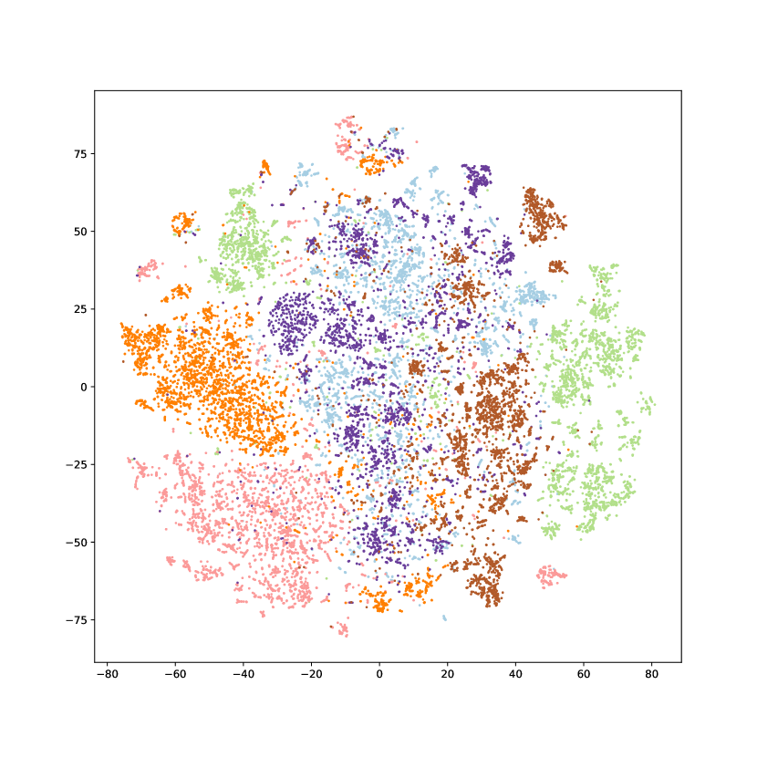
(a) Representations from pretrained checkpoint

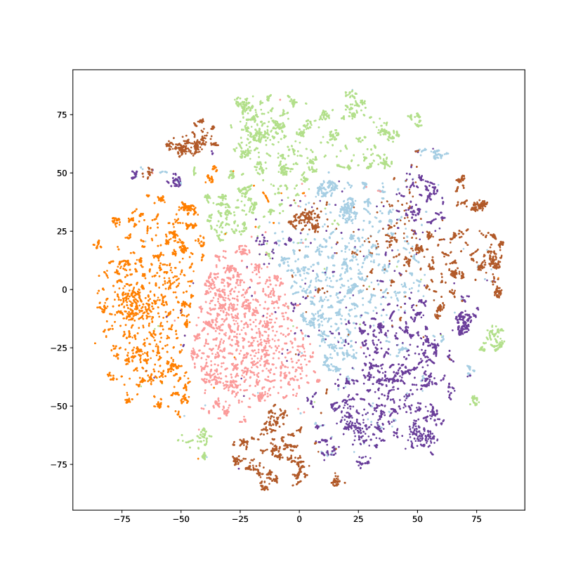
(b) Representations learned by S-MolSearch

Figure 2: t-SNE visualization of molecular representations learned by S-MolSearch versus pretrained checkpoint. Different colors represent different protein targets’ active molecules.

4.4.3 Impact of Labeled Data Scale

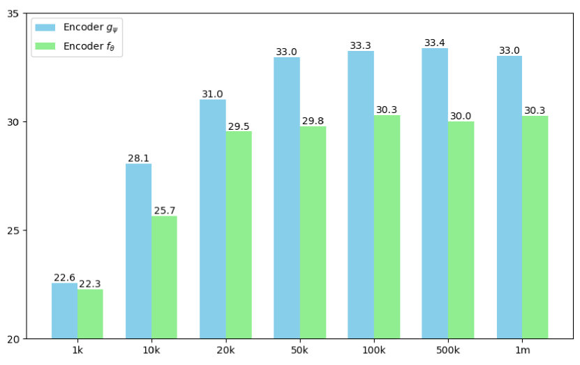
(a) EF 1% on DUD-E

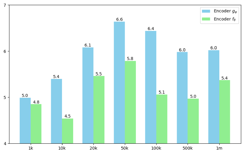
(b) EF 1% on LIT-PCBA

Figure 3: Performance on DUD-E and LIT-PCBA with varying numbers of labeled data, while keeping unlabeled data fixed at 1m. The blue bars represent the results of encoder $g_{\psi}$, while the green bars represent the results of encoder $f_{\theta}$.

In the molecular field, obtaining or creating labeled data can be expensive. We also analyze how the scale of labeled data affects the results. These results are derived from S-MolSearch trained with a 0.4 similarity threshold. As shown in Figure 3, experiments are conducted with varying amounts of labeled data, while keeping the unlabeled data fixed at 1 million. The performance of encoder $g_{\psi}$ improves as the amount of labeled data increases, especially when the absolute number of labeled data is limited. Additionally, the results of encoder $g_{\psi}$ are consistently higher than encoder $f_{\theta}$ trained using only labeled data. The best results are achieved with 50k and 100k labeled data, corresponding to labeled-to-unlabeled data ratios of 1:20 and 1:10, respectively. Beyond these amounts, increasing labeled data results in stable or slightly declining performance, suggesting that further improvements may necessitate an increase in unlabeled data or a reevaluation of hyperparameters. This trend helps us to find an optimal balance between labeled and unlabeled data to maximize efficiency and performance in S-MolSearch.

5 Conclusion

This study introduces S-MolSearch, a novel semi-supervised contrastive learning framework that significantly enhances the generalizability of machine learning models in virtual screening. Built on inverse optimal transport, S-MolSearch skillfully integrates limited labeled data with a vast reservoir of unlabeled data and excels at identifying potential drug candidates from extensive molecular libraries, substantially improving the accuracy and efficiency of molecule searches. This advancement addresses current challenges in virtual screening by facilitating efficient filtering of large datasets, highlighting the framework’s capability in scenarios where data annotation is costly.

Currently, S-MolSearch predominantly focuses on the molecular affinity data, omitting broader biochemical interactions, which suggests a potential area for improvement. Future work could integrate more extensive unsupervised datasets to further refine the framework’s effectiveness and explore additional applications in various bioinformatics fields.

Appendix A Data Curation Details

The data we used are manually extracted from regularly published primary literature, and then further curated and standardized. The whole ChEMBL database of version 33 is downloaded and cleaned via the following steps. The data is selected with assay type of ’B’, target type of ’SINGLE PROTEIN’, molecule type of ’Small molecule’, standard type of Ki, Kd, IC50, EC50 in nM, and standard relation of ’=’ and ’<’. Moreover, data with abnormal concentration value is further deleted, such as negative and unreasonable large ones.

Appendix B Metrics

We use the enrichment factor (EF) to evaluate the effectiveness of virtual screening methods. The calculation formula for EF is as follows:

$$\text{EF}=\frac{n_{a}/N_{x\%}}{n/N}$$

where $n$ represents the total number of active compounds in the database, $N$ represents the total number of molecules, $N_{x\%}$ represents the top $x\%$of all molecules, and $n_{a}$ represents the number of active compounds within the top $x\%$ of molecules."

Appendix C Proof for S-Molsearch Induced by Inverse Optimal Transport

First, we introduce a lemma to establish the relationship between IOT and contrastive learning from [51].

Lemma 3

The optimization problem 3 and 9 are equivalent:

$$\min_{\theta}KL(\hat{P}||P^{\theta})$$ (8)

$$\text{subject to}\quad\begin{aligned} &P^{\theta}=\arg\min_{P\in U(a)}\langle C^{\theta},P\rangle-\tau H(P)\end{aligned}$$

where $C^{\theta}\in R^{M\times N},C^{\theta}(i,j)=c-s_{ij}(\theta)$ and $\hat{P}(i,j)=\frac{\delta_{ij}}{n}$, $\delta$ denotes the Kronecker delta function.

$$\min_{\theta}-\sum_{i=1}^{n}log(\frac{exp(s_{ii}(\theta)/\tau)}{\sum_{j\neq i}exp(s_{ij}(\theta)/\tau)})$$ (9)

In addition, $P^{\theta}$ has the form as follows:

$$P^{\theta}=\frac{exp(s_{ii}(\theta)/\tau)}{\sum_{j\neq i}Nexp(s_{ij}(\theta)/\tau)}$$ (10)

C.1 Proof for Proposition 1

In the optimization problem 6, since the setting of $\mathcal{T}$ does not involve parameter optimization of $\theta$ or $\psi$, it is evident that the parameter optimization processes for $\theta$ and $\psi$ are independent. According to lemma 3, we can transform the original optimization problem into the following problem:

$$\min_{\theta,\psi}\left(KL(\Gamma^{g}||\Gamma^{\theta})+KL(\hat{\Gamma}^{\theta}||\Gamma^{\psi})+\mu Reg_{1}(\Gamma^{\psi})+\nu Reg_{2}(\Gamma^{\theta}))\right)$$ (11)

$$\text{subject to}\quad\begin{aligned} &\Gamma^{\theta}=\frac{exp(s_{ii}(\theta)/\tau)}{\sum_{j\neq i}Nexp(s_{ij}(\theta)/\tau)},\\ &\Gamma^{\psi}=\frac{exp(s_{ii}(\psi)/\tau)}{\sum_{j\neq i}Nexp(s_{ij}(\psi)/\tau)},\\ &\hat{\Gamma}^{\theta}=\mathcal{T}(f_{\theta}^{fixed},g_{\psi}^{fixed},X_{sup},X_{full})\end{aligned}$$

Due to

$$KL(p||q)=H(p,q)-H(p)$$ (12)

where $H(p)$ represents the entropy of $p$, and $H(p,q)$ represents the cross-entropy between $p$ and $q$. Given the selection of a specific $\mathcal{T}$ to derive $\hat{\Gamma}^{\theta}$, we can thus determine $\hat{\Gamma}^{\theta}(i,j)$ as a fixed quantity, making $H(p)$ constant. Furthermore, we can obtain

$$\min_{\theta,\psi}\Bigg{(}-\sum_{i=1}^{n}\log\left(\frac{\exp(s_{ii}(\theta)/\tau)}{\sum_{j\neq i}\exp(s_{ij}(\theta)/\tau)}\right)$$ (13)

$$\qquad-\sum_{i=1}^{n}\sum_{j=1}^{n}\hat{\Gamma}^{\theta}(i,j)\log\left(\frac{\exp(s_{ij}(\psi)/\tau)}{\sum_{k\neq i}\exp(s_{ik}(\psi)/\tau)}\right)$$

$$\qquad+\mu\,\mathrm{Reg}_{1}(\Gamma^{\psi})+\nu\,\mathrm{Reg}_{2}(\Gamma^{\theta})\Bigg{)}$$

$$\text{where}\quad\begin{aligned} \hat{\Gamma}^{\theta}(i,j)=\mathcal{T}(f_{\theta}^{\text{fixed}},g_{\psi}^{\text{fixed}},X_{\text{sup}},X_{\text{full}})_{(i,j)}\end{aligned}$$

C.2 Proof for Proposition 2

Since $C^{\theta^{fixed}}$ does not involve parameter optimization of $\theta$, we can still calculate the value of $\hat{\Gamma}^{\theta}(i,j)$. According to the proof in C.1, we know that

$$\min_{\theta,\psi}\Bigg{(}-\sum_{i=1}^{n}\log\left(\frac{\exp(s_{ii}(\theta)/\tau)}{\sum_{j\neq i}\exp(s_{ij}(\theta)/\tau)}\right)$$ (14)

$$\qquad-\sum_{i=1}^{n}\sum_{j=1}^{n}\hat{\Gamma}^{\theta}(i,j)\log\left(\frac{\exp(s_{ij}(\psi)/\tau)}{\sum_{k\neq i}\exp(s_{ik}(\psi)/\tau)}\right)$$

$$\qquad+\mu\,\mathrm{Reg}_{1}(\Gamma^{\psi}))\Bigg{)}$$

$$\text{where}\quad\begin{aligned} \hat{\Gamma}^{\theta}(i,j)=\arg\min_{\Gamma\in U(a,b),\,a=\mathbf{1}_{N},\,b=\mathbf{1}_{N}}\left(\langle C^{\theta^{\text{fixed}}},\Gamma\rangle+\frac{\lambda}{2}\|\Gamma\|^{2}\right)_{(i,j)}\end{aligned}$$

When we choose $\mathrm{Reg}_{1}$ as the regularization term 4, we obtain the optimization formulation of S-MolSearch.

Appendix D Reproduce details

For the training of S-MolSearch , we use Adam optimizer at a learning rate of 0.001. The batch size is 128, and the training is conducted on 4 NVIDIA V100 32G GPUs. For backbone model, we use the same parameters as Uni-Mol. We randomly sample data from the labeled and unlabeled datasets to form the validation set, and select checkpoints based on the loss. More detailed configurations can be found in the code repository.

Appendix E Limitations

S-MolSearch falls short in terms of interpretability. Traditional 3D molecule search methods can capture shape and functional features required for biological interactions, providing scientists with mechanistic insights. S-MolSearch is currently unable to provide such intuitive insights for molecule search.

Appendix F Potential societal impacts

S-MolSearch performs well on LBVS and can help screen bioactive molecules from large molecule databases. This eases the workload of medicinal chemists and may accelerate the discovery of new drug. On the downside, S-MolSearch also runs the risk of being used inappropriately, such as when it is used to search for similar molecules to drugs that are addictive.

References

- [1] Gerhard Klebe. Virtual ligand screening: strategies, perspectives and limitations. Drug discovery today, 11(13-14):580–594, 2006.
- [2] Hongbin Huang, Guigui Zhang, Yuquan Zhou, Chenru Lin, Suling Chen, Yutong Lin, Shangkang Mai, and Zunnan Huang. Reverse screening methods to search for the protein targets of chemopreventive compounds. Frontiers in chemistry, 6:138, 2018.
- [3] Dominique Sydow, Lindsey Burggraaff, Angelika Szengel, Herman WT van Vlijmen, Adriaan P IJzerman, Gerard JP van Westen, and Andrea Volkamer. Advances and challenges in computational target prediction. Journal of chemical information and modeling, 59(5):1728–1742, 2019.
- [4] Berin Karaman and Wolfgang Sippl. Computational drug repurposing: current trends. Current medicinal chemistry, 26(28):5389–5409, 2019.
- [5] Xuan-Yu Meng, Hong-Xing Zhang, Mihaly Mezei, and Meng Cui. Molecular docking: a powerful approach for structure-based drug discovery. Current computer-aided drug design, 7(2):146–157, 2011.
- [6] Wenchao Lu, Rukang Zhang, Hao Jiang, Huimin Zhang, and Cheng Luo. Computer-aided drug design in epigenetics. Frontiers in chemistry, 6:57, 2018.
- [7] Thomas A Halgren, Robert B Murphy, Richard A Friesner, Hege S Beard, Leah L Frye, W Thomas Pollard, and Jay L Banks. Glide: a new approach for rapid, accurate docking and scoring. 2. enrichment factors in database screening. Journal of medicinal chemistry, 47(7):1750–1759, 2004.
- [8] Oleg Trott and Arthur J Olson. Autodock vina: improving the speed and accuracy of docking with a new scoring function, efficient optimization, and multithreading. Journal of computational chemistry, 31(2):455–461, 2010.
- [9] Hakime Öztürk, Arzucan Özgür, and Elif Ozkirimli. Deepdta: deep drug–target binding affinity prediction. Bioinformatics, 34(17):i821–i829, 2018.
- [10] Liangzhen Zheng, Jingrong Fan, and Yuguang Mu. Onionnet: a multiple-layer intermolecular-contact-based convolutional neural network for protein–ligand binding affinity prediction. ACS omega, 4(14):15956–15965, 2019.
- [11] Marta M Stepniewska-Dziubinska, Piotr Zielenkiewicz, and Pawel Siedlecki. Development and evaluation of a deep learning model for protein–ligand binding affinity prediction. Bioinformatics, 34(21):3666–3674, 2018.
- [12] Bowen Gao, Bo Qiang, Haichuan Tan, Yinjun Jia, Minsi Ren, Minsi Lu, Jingjing Liu, Wei-Ying Ma, and Yanyan Lan. Drugclip: Contrasive protein-molecule representation learning for virtual screening. Advances in Neural Information Processing Systems, 36, 2024.
- [13] Viet-Khoa Tran-Nguyen, Célien Jacquemard, and Didier Rognan. Lit-pcba: an unbiased data set for machine learning and virtual screening. Journal of chemical information and modeling, 60(9):4263–4273, 2020.
- [14] Paul CD Hawkins, A Geoffrey Skillman, and Anthony Nicholls. Comparison of shape-matching and docking as virtual screening tools. Journal of medicinal chemistry, 50(1):74–82, 2007.
- [15] G Madhavi Sastry, Steven L Dixon, and Woody Sherman. Rapid shape-based ligand alignment and virtual screening method based on atom/feature-pair similarities and volume overlap scoring. Journal of chemical information and modeling, 51(10):2455–2466, 2011.
- [16] Jonatan Taminau, Gert Thijs, and Hans De Winter. Pharao: pharmacophore alignment and optimization. Journal of Molecular Graphics and Modelling, 27(2):161–169, 2008.
- [17] Xin Yan, Jiabo Li, Zhihong Liu, Minghao Zheng, Hu Ge, and Jun Xu. Enhancing molecular shape comparison by weighted gaussian functions. Journal of chemical information and modeling, 53(8):1967–1978, 2013.
- [18] Ambrish Roy and Jeffrey Skolnick. Ligsift: an open-source tool for ligand structural alignment and virtual screening. Bioinformatics, 31(4):539–544, 2014.
- [19] Xiaofeng Liu, Hualiang Jiang, and Honglin Li. Shafts: a hybrid approach for 3d molecular similarity calculation. 1. method and assessment of virtual screening. Journal of chemical information and modeling, 51(9):2372–2385, 2011.
- [20] Weiqiang Lu, Xiaofeng Liu, Xianwen Cao, Mengzhu Xue, Kangdong Liu, Zhenjiang Zhao, Xu Shen, Hualiang Jiang, Yufang Xu, Jin Huang, et al. Shafts: a hybrid approach for 3d molecular similarity calculation. 2. prospective case study in the discovery of diverse p90 ribosomal s6 protein kinase 2 inhibitors to suppress cell migration. Journal of medicinal chemistry, 54(10):3564–3574, 2011.
- [21] Dilyana Dimova and Jürgen Bajorath. Advances in activity cliff research. Molecular informatics, 35(5):181–191, 2016.
- [22] Michael M Mysinger, Michael Carchia, John J Irwin, and Brian K Shoichet. Directory of useful decoys, enhanced (dud-e): better ligands and decoys for better benchmarking. Journal of medicinal chemistry, 55(14):6582–6594, 2012.
- [23] Ting Chen, Simon Kornblith, Mohammad Norouzi, and Geoffrey Hinton. A simple framework for contrastive learning of visual representations. In International conference on machine learning, pages 1597–1607. PMLR, 2020.
- [24] Kaiming He, Haoqi Fan, Yuxin Wu, Saining Xie, and Ross Girshick. Momentum contrast for unsupervised visual representation learning. In Proceedings of the IEEE/CVF conference on computer vision and pattern recognition, pages 9729–9738, 2020.
- [25] Alec Radford, Jong Wook Kim, Chris Hallacy, Aditya Ramesh, Gabriel Goh, Sandhini Agarwal, Girish Sastry, Amanda Askell, Pamela Mishkin, Jack Clark, et al. Learning transferable visual models from natural language supervision. In International Conference on Machine Learning, pages 8748–8763. PMLR, 2021.
- [26] Jean-Bastien Grill, Florian Strub, Florent Altché, Corentin Tallec, Pierre Richemond, Elena Buchatskaya, Carl Doersch, Bernardo Avila Pires, Zhaohan Guo, Mohammad Gheshlaghi Azar, et al. Bootstrap your own latent-a new approach to self-supervised learning. Advances in neural information processing systems, 33:21271–21284, 2020.
- [27] Andrew M Stuart and Marie-Therese Wolfram. Inverse optimal transport. SIAM Journal on Applied Mathematics, 80(1):599–619, 2020.
- [28] Anna Gaulton, Louisa J Bellis, A Patricia Bento, Jon Chambers, Mark Davies, Anne Hersey, Yvonne Light, Shaun McGlinchey, David Michalovich, Bissan Al-Lazikani, et al. Chembl: a large-scale bioactivity database for drug discovery. Nucleic acids research, 40(D1):D1100–D1107, 2012.
- [29] Matthew Ragoza, Joshua Hochuli, Elisa Idrobo, Jocelyn Sunseri, and David Ryan Koes. Protein–ligand scoring with convolutional neural networks. Journal of chemical information and modeling, 57(4):942–957, 2017.
- [30] Peter Willett. Similarity-based virtual screening using 2d fingerprints. Drug discovery today, 11(23-24):1046–1053, 2006.
- [31] Xin Yan, Qiong Gu, Feng Lu, Jiabo Li, and Jun Xu. Gsa: a gpu-accelerated structure similarity algorithm and its application in progressive virtual screening. Molecular diversity, 16:759–769, 2012.
- [32] Alan Geoffrey Wilson. The use of entropy maximising models, in the theory of trip distribution, mode split and route split. Journal of transport economics and policy, pages 108–126, 1969.
- [33] Richard Sinkhorn. Diagonal equivalence to matrices with prescribed row and column sums. The American Mathematical Monthly, 74(4):402–405, 1967.
- [34] Mathieu Blondel, Vivien Seguy, and Antoine Rolet. Smooth and sparse optimal transport, 2018.
- [35] Wei-Ting Chiu, Pei Wang, and Patrick Shafto. Discrete probabilistic inverse optimal transport. In International Conference on Machine Learning, pages 3925–3946. PMLR, 2022.
- [36] Arnaud Dupuy, Alfred Galichon, and Yifei Sun. Estimating matching affinity matrix under low-rank constraints. arXiv preprint arXiv:1612.09585, 2016.
- [37] Ruilin Li, Xiaojing Ye, Haomin Zhou, and Hongyuan Zha. Learning to match via inverse optimal transport. Journal of machine learning research, 20(80):1–37, 2019.
- [38] Semi-Supervised Learning. Semi-supervised learning. CSZ2006. html, 5, 2006.
- [39] David Berthelot, Nicholas Carlini, Ian Goodfellow, Nicolas Papernot, Avital Oliver, and Colin A Raffel. Mixmatch: A holistic approach to semi-supervised learning. Advances in neural information processing systems, 32, 2019.
- [40] Qizhe Xie, Minh-Thang Luong, Eduard Hovy, and Quoc V Le. Self-training with noisy student improves imagenet classification. In Proceedings of the IEEE/CVF conference on computer vision and pattern recognition, pages 10687–10698, 2020.
- [41] Mahmoud Assran, Mathilde Caron, Ishan Misra, Piotr Bojanowski, Armand Joulin, Nicolas Ballas, and Michael Rabbat. Semi-supervised learning of visual features by non-parametrically predicting view assignments with support samples. In Proceedings of the IEEE/CVF International Conference on Computer Vision, pages 8443–8452, 2021.
- [42] Dong-Hyun Lee et al. Pseudo-label: The simple and efficient semi-supervised learning method for deep neural networks. In Workshop on challenges in representation learning, ICML, volume 3, page 896. Atlanta, 2013.
- [43] Samuli Laine and Timo Aila. Temporal ensembling for semi-supervised learning. arXiv preprint arXiv:1610.02242, 2016.
- [44] Mamshad Nayeem Rizve, Kevin Duarte, Yogesh S Rawat, and Mubarak Shah. In defense of pseudo-labeling: An uncertainty-aware pseudo-label selection framework for semi-supervised learning. In International Conference on Learning Representations, 2020.
- [45] Subhabrata Mukherjee and Ahmed Awadallah. Uncertainty-aware self-training for few-shot text classification. Advances in Neural Information Processing Systems, 33:21199–21212, 2020.
- [46] Sangwoo Mo, Minkyu Kim, Kyungmin Lee, and Jinwoo Shin. S-clip: Semi-supervised vision-language learning using few specialist captions. Advances in Neural Information Processing Systems, 36, 2024.
- [47] Gengmo Zhou, Zhifeng Gao, Qiankun Ding, Hang Zheng, Hongteng Xu, Zhewei Wei, Linfeng Zhang, and Guolin Ke. Uni-mol: A universal 3d molecular representation learning framework. In The Eleventh International Conference on Learning Representations, 2023.
- [48] Rémi Flamary, Nicolas Courty, Alexandre Gramfort, Mokhtar Z. Alaya, Aurélie Boisbunon, Stanislas Chambon, Laetitia Chapel, Adrien Corenflos, Kilian Fatras, Nemo Fournier, Léo Gautheron, Nathalie T.H. Gayraud, Hicham Janati, Alain Rakotomamonjy, Ievgen Redko, Antoine Rolet, Antony Schutz, Vivien Seguy, Danica J. Sutherland, Romain Tavenard, Alexander Tong, and Titouan Vayer. Pot: Python optimal transport. Journal of Machine Learning Research, 22(78):1–8, 2021.
- [49] Alexandre Sablayrolles, Matthijs Douze, Cordelia Schmid, and Hervé Jégou. Spreading vectors for similarity search. arXiv preprint arXiv:1806.03198, 2018.
- [50] Maxime Oquab, Timothée Darcet, Théo Moutakanni, Huy Vo, Marc Szafraniec, Vasil Khalidov, Pierre Fernandez, Daniel Haziza, Francisco Massa, Alaaeldin El-Nouby, et al. Dinov2: Learning robust visual features without supervision. arXiv preprint arXiv:2304.07193, 2023.
- [51] Liangliang Shi, Gu Zhang, Haoyu Zhen, Jintao Fan, and Junchi Yan. Understanding and generalizing contrastive learning from the inverse optimal transport perspective. In International conference on machine learning, pages 31408–31421. PMLR, 2023.
- [52] Maria Hauser, Martin Steinegger, and Johannes Söding. Mmseqs software suite for fast and deep clustering and searching of large protein sequence sets. Bioinformatics, 32(9):1323–1330, 2016.
- [53] Michael Brocidiacono, Paul Francoeur, Rishal Aggarwal, Konstantin I Popov, David Ryan Koes, and Alexander Tropsha. Bigbind: learning from nonstructural data for structure-based virtual screening. Journal of Chemical Information and Modeling, 64(7):2488–2495, 2023.
- [54] Xiangying Zhang, Haotian Gao, Haojie Wang, Zhihang Chen, Zhe Zhang, Xinchong Chen, Yan Li, Yifei Qi, and Renxiao Wang. Planet: a multi-objective graph neural network model for protein–ligand binding affinity prediction. Journal of Chemical Information and Modeling, 2023.
- [55] Russell Spitzer and Ajay N Jain. Surflex-dock: Docking benchmarks and real-world application. Journal of computer-aided molecular design, 26:687–699, 2012.
- [56] Andrew T McNutt, Paul Francoeur, Rishal Aggarwal, Tomohide Masuda, Rocco Meli, Matthew Ragoza, Jocelyn Sunseri, and David Ryan Koes. Gnina 1.0: molecular docking with deep learning. Journal of cheminformatics, 13(1):43, 2021.
- [57] Zhenla Jiang, Jianrong Xu, Aixia Yan, and Ling Wang. A comprehensive comparative assessment of 3d molecular similarity tools in ligand-based virtual screening. Briefings in bioinformatics, 22(6):bbab231, 2021.