Comment on
Room-temperature spontaneous superradiance from single diamond nanocrystals [Nat. Commun. 8, 1205 (2017)]

Abstract

The paper by C. Bradac et al. [Nat. Commun. 8, 1205 (2017)] discusses room-temperature superradiance from NV color centers in diamonds. It presents a new model intended to reflect experimental characteristics of this phenomenon. To validate the model, the authors provide experimental results that are subsequently compared with numerical calculations derived from the scheme. Motivated by our own experiments with the fluorescence of similar NV samples, we attempted to create a theoretical model to accurately describe experimental systems. Initially, we aimed to incorporate the numerical equations from Bradac et al.’s paper’s supplement into our own theoretical framework. However, we encountered numerous issues resulting in non-physical results such as negative photon counts or non-zero asymptotic fluorescence intensity. We identified these inconsistencies and proposed amendments to rectify them. We have developed our own framework by correctly reinterpreting the terms of the master equation. The resulting formulas produce physically meaningful results consistent with experimental data.

I Introduction

The paper by C. Bradac et al. [1], supplemented with additional material [2], reports on an experiment investigating superradiance in nanodiamond samples at room temperature. The study introduces a theoretical model accompanied by numerical simulations that reportedly reflect the experimental findings. While we refrain from commenting on the experimental procedures, as they are beyond the scope of our verification, we present evidence indicating the inadequacy of the theoretical model presented in [1, 2]. It comprises equations yielding results inconsistent with both the reported experimental data and basic physical principles. In our investigation, we identify numerous instances of non-physical behavior within the model and propose alternative equations along with their interpretations. Our revised model not only yields physically meaningful results but also demonstrates better alignment with the experimental data presented in Ref. [1].

The structure of this work is outlined as follows. We begin with Section II by providing a concise review of the model proposed in Ref. [1]. Here, we present the principal equations along with explanations of the associated symbols. Subsequently, in Section III, we present the examination of a scenario involving seven color centers, which is identical to the case explored in Ref. [1]. By employing computational software to implement the model, we obtain results that diverge from those presented in the aforementioned study. While we specifically discuss one case in Section III, other examples of discrepancies are detailed in the Appendix B. Furthermore, in Section IV, we propose equations that offer an accurate mathematical representation of the phenomenon under consideration. Through our proposed equations, we demonstrate that the instances previously misrepresented according to the model from Ref. [1], now exhibit all required physical properties. Additionally, the fluorescence plots generated from our model show characteristic emission patterns. Complementing our study is an Appendix A, where we provide comments on individual corrected elements of the equations and elaborate on their proposed interpretations. Notably, errors within the model from Ref. [1] appear to be of various kinds; some may stem from computational inaccuracies, while others may originate from flawed physical premises.

For clarity and consistency, we introduce a convention to discern between models. The formalism outlined in the supplementary material [2] to Ref. [1] is referred to as Model A, while we designate the framework introduced in the present paper as Model B. We adhere to this delineation throughout the remainder of this text.

II Model A

The research discussed in Ref. [1], as well as in our laboratory, involves diamond samples containing lattice defects where a nitrogen atom and a vacancy replace a pair of carbon atoms. These centers are subsequently excited by light, and the resulting spontaneous emission is observed. To facilitate a comparative analysis, we adopt identical labeling and experimental approaches as outlined in the referenced work[1]. Specifically, we partition the diamond into distinct domains denoted by $\sigma$, each containing a certain number of color centers $N_{\sigma}$, contributing to the total count $N$.

The foundational equation in constructing Model A is the Gorini-Kossakowski-Lindblad-Sudarshan (GKLS) master equation [3, 4, 5, 6], which encompasses both nonphenomenological and phenomenological terms. These terms are expected to capture the intricacies of collective state defocusing and intersystem crossing phenomena within the context of superradiance. Each term in the equation is associated with constants $\gamma$, which are indicative of the characteristic rates governing these phenomena. These constants are devised analogously to the conventional decay rate, denoted as $\gamma^{(\sigma)}$, which typifies the spontaneous emission behavior of a single atom.

Let us recapture the version of the GKLS equation with phenomenological factors following Ref. [2]:

$$\frac{d}{dt}P_{J,M}^{(\sigma)}(t)=\gamma\Biggl{[}(J(J+1)-M(M+1))P_{J,M+1}^{(\sigma)}(t)-(J(J+1)-M(M-1))P_{J,M}^{(\sigma)}(t)\Biggl{]}$$ (1)

$$-\color[rgb]{0,0,0}\underbrace{\color[rgb]{1,0,0}2J}_{\color[rgb]{0,0,0}\scalebox{1.1}{(A)}}\gamma_{d}^{\sigma}\Biggl{[}{\underbrace{\color[rgb]{1,0,0}1}_{\color[rgb]{0,0,0}\scalebox{1.1}{(B)}}\color[rgb]{1,0,0}\color[rgb]{0,0,0}\underbrace{\color[rgb]{1,0,0}{{{\biggl{(}1-\biggl{|}\frac{M}{J}\biggl{|}^{2}\biggl{)}}}}}_{\color[rgb]{0,0,0}\scalebox{1.1}{(C)}}}P_{J,M}^{(\sigma)}(t){\color[rgb]{0,0,0}\underbrace{\color[rgb]{1,0,0}+2}_{\scalebox{1.1}{(D)}}}\Bigl{(}J+\frac{1}{2}\Bigl{)}{\color[rgb]{1,0,0}\color[rgb]{0,0,0}\underbrace{\color[rgb]{1,0,0}{\biggl{(}1-\biggl{|}\frac{M+\frac{1}{2}}{J+\frac{1}{2}}\biggl{|}^{2}\biggl{)}}}_{{\scalebox{1.1}{(E)}}}}P_{J+\frac{1}{2},M+\frac{1}{2}}^{(\sigma)}(t)\Biggl{]}$$

$$+\gamma_{ISC}^{\sigma}\Biggl{[}\underbrace{\color[rgb]{1,0,0}(J+M+1)}_{\scalebox{1.1}{(F)}}P_{J+\frac{1}{2},M+\frac{1}{2}}^{(\sigma)}(t)-\underbrace{\color[rgb]{1,0,0}(J+M)}_{\scalebox{1.1}{(G)}}P_{J,M}^{(\sigma)}(t)\Biggl{]}.$$

In Eq. (1), we have highlighted specific terms using red font and labeled them with consecutive letters using brackets. These terms are identified as flawed and necessitate modification. By marking them in this manner, we facilitate precise and convenient reference and commentary on these terms in subsequent sections of the article

At this point, we explain all undefined yet notations appearing in the aforementioned equation and in all subsequent equations. To facilitate seamless comparison and ensure clarity, we adopt a convention identical to that of Ref.[1]:

$\bullet P_{J,M}^{(\sigma)}$ denotes the population of the collective state with the numbers $J$ and $M$ in the collective space,
$\bullet\gamma$ represents the decay constant,
$\bullet\gamma_{ISC}^{\sigma}$ signifies the so-called intersystem crossing (ISC) rate,
$\bullet\gamma_{d}^{\sigma}$ refers to the dephasing rate,
$\bullet N_{nc}^{(\sigma)}$ stands for the number of independently radiating emitters (exponentially) at time t
$\bullet F_{N_{\sigma}}$ represents the fluorescence at a given time t,
$\bullet$ $N$ signifies the total number of emitters.

The second important formula provides the number of non-radiative decaying emitters – denoted by $N_{nc}$ (Eq. 13 in Ref. [SupplementNature]), which takes the form:

$$\frac{d}{dt}N_{nc}^{(\sigma)}=-(\gamma+\gamma_{ISC}^{\sigma})N_{nc}^{(\sigma)}(t)+\gamma_{d}^{\sigma}\sum_{J=\frac{1}{2}}^{\frac{N}{2}}\sum_{M=-J}^{J}\underbrace{\color[rgb]{1,0,0}\biggl{(}1-\Bigl{|}\frac{M}{J}\Bigl{|}^{2}\biggl{)}}_{\scalebox{1.1}{(H)}}2JP_{J,M}^{(\sigma)},$$ (2)

where a specific term has been highlighted for reference.

The last key equation describes the fluorescence rate (Eq. 15 in Ref. [2]) and takes the form:

$$F_{N_{\sigma}}(t)=\gamma\Bigl{(}N_{nc}^{(\sigma)}(t)+\sum_{J=\frac{1}{2}}^{\frac{N}{2}}\sum_{M=-J}^{J}\bigl{(}J(J+1)-\underbrace{\color[rgb]{1,0,0}M(M+1)}_{\scalebox{1.1}{(I)}}\bigl{)}P_{J,M}^{(\sigma)}\Bigl{)}.$$ (3)

These three equations are fundamental for the results presented in Ref. [1]. Eq. 1 describes the dynamics of the occupation of collective states $\ket{J,M,\sigma}$ with quantum numbers $J,M$ under the influence of mechanisms such as spontaneous emission, dephasing, or radiative transitions. Eq. 2 describes the population of emitters that radiate light according to the exponential decay law outlined in the Weiskopf-Wigner theory [7]. The effects of dephasing on the collective state of the color centers in the diamond lead to an increase in the number of such emitters, resulting in a decrease in the number of collectively emitting emitters. Eq. 3 describes the fluorescence of light based on predictions of the population of collectively and standardly emitting emitters. With such tools, the intensity of light can be plotted and observed.

III Model A: Critical assessment

In this paragraph, we present fluorescence plots generated from analytical formulas provided in Ref.[2]. For consistency, we employ identical parameters as those specified in Refs. [1, 2]. By juxtaposing the obtained results with the data and simulations from Ref. [1], we aim to visually demonstrate the inaccuracies of Model A. Given that a single clear discrepancy suffices, we show the case involving $7$ color centers. We have also tested examples involving $2$ and $10$ centers, both of which exhibit inconsitencies. However, to keep the present section concise, these findings shall be presented in Appendix B.

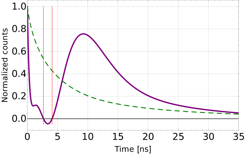
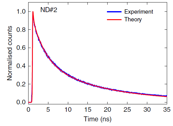
Figure 1: In the Figure on the left one can see two simulation variants of fluorescence intensity in time, from $0$ to $35$ ns, for 7 NV centers. The purple solid line represents the result of Model A [1, SupplementNature], while the green dashed line represents Model B introduced in the present paper. The figure on the right side is taken from Ref. [1] and presents the simulation results of Model A against experimental data.

In the scenario involving 7 color centers ($N=7$), we implemented Models A and B, and the corresponding results are depicted in Fig. 1 on the left side. In this plot, the solid line corresponds to Model A. One can notice that the observed fluorescence pattern does not align with the expected behavior of Dicke’s superradiance, which is the focus of our discussion. Instead, we observe intense fluorescence from the initial moment, reaching a maximum value of 1 for $t=0$, and then declining rapidly. The plot generated from Model A appears strikingly different from the results provided in Ref. [1] for the same parameters, cf. Fig. 1 on the right side. Notably, our simulations using Model B, represented by the dashed line in Fig. 1 on the left side, yielded contrasting plots compared to those obtained by Model A.

Additionally, we encountered instances of unphysical behavior in the simulation results generated by Model A. Specifically, we observed that the fluorescence intensity dropped below zero within a certain time interval, as indicated by the vertical lines in Fig. 1 on the left side. Furthermore, an unphysical non-zero asymptote was obtained. To further examine this phenomenon, we extended the time range, as illustrated in Fig. 4, which is provided in Appendix B.

IV Model B: Superadiance from a single diamond nanocrystal

According to our research, the proper master equation for fluorescence modeling reads:

$$\frac{d}{dt}P_{J,M}^{(\sigma)}(t)=\gamma\Biggl{[}(J(J+1)-M(M+1))P_{J,M+1}^{(\sigma)}(t)-(J(J+1)-M(M-1))P_{J,M}^{(\sigma)}(t)\Biggl{]}-\gamma_{d}^{\sigma}\Biggl{[}2J{\biggl{|}\frac{M}{J}\biggl{|}^{2}}P_{J,M}^{(\sigma)}(t){\color[rgb]{0,0,0}}$$ (4)

$$-2\Bigl{(}J+\frac{1}{2}\Bigl{)}{\biggl{|}\frac{M+\frac{1}{2}}{J+\frac{1}{2}}\biggl{|}^{2}}P_{J+\frac{1}{2},M+\frac{1}{2}}^{(\sigma)}(t)\Biggl{]}+\gamma_{ISC}^{\sigma}\Biggl{[}(J+M+1)(J-M+1)P_{J+\frac{1}{2},M+\frac{1}{2}}^{(\sigma)}(t)-(J+M)(J-M+1)P_{J,M}^{(\sigma)}(t)\Biggl{]}.$$

Of particular significance are the initial conditions we imposed on populating states within the collective space. We followed the same approach as the authors of the referenced work [1, 2], assuming an even distribution of color centers across individual states. Consequently, the initial state of the total system of color centers is described as follows:

$$\hat{\rho}^{(\sigma)}(0)=\sum_{N_{\sigma}}p_{N_{\sigma}}\hat{\rho}_{N_{\sigma}}^{(\sigma)}(0),$$ (5)

where $p_{N_{\sigma}}$ represents the probability that a domain of color centers, characterized by its size $N_{\sigma}$, exists with the spin $\sigma$. The summation over these probabilities yields the probability of having a total spin $\sigma$, i.e. $\sum_{N_{\sigma}}p_{N_{\sigma}}=p_{\sigma}$. The properties of the density matrix $\hat{\rho}_{N_{\sigma}}^{(\sigma)}(0)$ should be further explained. It can be decomposed as a statistical mixture over projectors on Dicke states $\ket{J,M,\sigma}\bra{J,M,\sigma}$:

$$\hat{\rho}^{(\sigma)}_{N_{\sigma}}(0)=\sum_{M}P^{(\sigma)}_{J=\frac{N_{\sigma}}{2},M}(0)\ket{\frac{N_{\sigma}}{2},M,\sigma}\bra{\frac{N_{\sigma}}{2},M,\sigma},$$ (6)

where the occupation probability in subspaces, $P_{J=\frac{N_{\sigma}}{2},M}^{(\sigma)}(0)$, is equal to $(N_{{\sigma}}+1)^{-1}$. Additionally, we sum over the two possible values of spin projection, resulting in $\sum_{\sigma=0,1}p_{\sigma}=1$. Following Ref. [1], we treat cases with spin projection $\pm 1$ as indistinguishable.

The number of independently emitting color centers increases proportionally to the parameter $\gamma_{d}^{\sigma}$ responsible for dephasing, accompanied by the appropriate probability coefficients. We have provided a deeper discussion about these quantities in Appendix A. For now, let us introduce the differential equation governing the population decay of independently radiating color centers, which is known for its exponential nature

$$\frac{d}{dt}N_{nc}^{(\sigma)}=-(\gamma+\gamma_{ISC}^{\sigma})N_{nc}^{(\sigma)}(t)+\gamma_{d}^{\sigma}\sum_{J=\frac{1}{2}}^{\frac{N}{2}}\sum_{M=-J}^{J}\left|\frac{M}{J}\right|^{2}2J\,P_{J,M}^{(\sigma)}.$$ (7)

The most crucial quantity for fluorescence modeling, which is also an important component of Ref. [1], is the total (from all domains) fluorescence intensity, which can be determined from the following equation:

$$F_{N_{\sigma}}(t)=\gamma\Bigl{(}N_{nc}^{(\sigma)}(t)+\sum_{J=\frac{1}{2}}^{\frac{N}{2}}\sum_{M=-J}^{J}\bigl{(}J(J+1)-M(M-1)\bigl{)}P_{J,M}^{(\sigma)}\Bigl{)}.$$ (8)

The numerical algorithms need to be developed, a task to be executed in the subsequent software implementation. What remains to be described is the structure of the states comprising our physical system. The states are derived from Ref. [1] and are implemented in our numerical simulations, as detailed in Appendix B.

A comprehensive presentation and comparison of the master equations from Models A and B are provided in detail in Appendix A. Additionally, solid arguments supporting the need for significant and conceptual modifications of the theoretical framework proposed in Refs. [1, 2] are presented.

V Discussion

In this paper, we have presented a critical assessment of the theoretical model proposed in Ref. [1], labeled as Model A, regarding room-temperature superradiance from NV color centers in diamonds. We presented correct equations, Model B, which when evaluated by numerical means provide physically meaningful results aligned with experimental data.

Our investigation revealed several key findings that challenge the validity of the Model A. Firstly, we observed significant discrepancies between the simulated fluorescence patterns obtained from Model A and those reported in Ref. [1]. These discrepancies were particularly pronounced in scenarios involving a small number of color centers, such as the case of $N=7$ emitters, where our simulations yielded markedly different results from those published in Ref. [1].

Furthermore, we identified instances of unphysical behavior in the simulations generated based on Model A. Specifically, we observed cases, where the normalized counts dropped below zero and an unphysical non-zero asymptote was obtained. These findings raise doubts about the precision and reliability of Model A in accurately describing the physical behavior of the system under consideration.

Our critique extends beyond demonstrating numerical discrepancies and unphysical behavior. We also provided the correct model that remains in agreement with physical assumptions related to fluoresence. By rigorously comparing our theory with the framework given in Ref. [1], we aimed to provide a comprehensive analysis of the shortcomings and limitations of Model A.

It is important to note that while our critique challenges the validity of Model A, it does not negate the significance of the experimental findings reported in Ref. [1]. Experimental results play a crucial role in advancing our understanding of complex physical phenomena, and the discrepancies identified in the theoretical framework demonstrate the need for further refinement and validation of modeling.

Disclosures. The authors declare no conflicts of interest.

Data availability statement. This manuscript has no associated data. The data statement is not applicable to this article as no datasets were generated or analyzed during the current study.

Code availability statement. The code associated with this study can be obtained from the corresponding author upon reasonable request.

Appendix A Comparison of the equations in Models A and B

In Eq. (1), we have identified terms that differ from those in Eq. (4) by highlighting them in red and enclosing them in brackets. Each term is labeled alphabetically. Tab. 1 provides a reference to each faulty term along with the correct replacement.

Term label	Model A	Model B
A	${\color[rgb]{1,0,0}2J}$	${\color[rgb]{0,0,1}1}$
B	${\color[rgb]{1,0,0}{1}}$	${\color[rgb]{0,0,1}{2J}}$
C	${\color[rgb]{1,0,0}{1-\biggl{|}\frac{M}{J}\biggl{|}^{2}}}$	${\color[rgb]{0,0,1}{\bigl{|}}\frac{M}{J}{\bigl{|}}^{2}}$
D	${\color[rgb]{1,0,0}+2}$	${\color[rgb]{0,0,1}-2}$
E	${\color[rgb]{1,0,0}{1-\biggl{|}\frac{M+\frac{1}{2}}{J+\frac{1}{2}}\biggl{|}^{2}}}$	${\color[rgb]{0,0,1}{\biggl{|}}\frac{M+\frac{1}{2}}{J+\frac{1}{2}}{\biggl{|}}^{2}}$
F	${\color[rgb]{1,0,0}(J+M+1)}$	${\color[rgb]{0,0,1}(J+M+1)(J-M+1)}$
G	${\color[rgb]{1,0,0}(J+M)}$	${\color[rgb]{0,0,1}(J+M)(J-M+1)}$
H	${\color[rgb]{1,0,0}1-\Bigl{|}\frac{M}{J}\Bigl{|}^{2}}$	${\color[rgb]{0,0,1}\Bigl{|}\frac{M}{J}\Bigl{|}^{2}}$
I	${\color[rgb]{1,0,0}M(M+1)}$	${\color[rgb]{0,0,1}M(M-1)}$

Table 1: The comparison of the Model A and Model B. The labels, A-G, H, I, refer to the identified parts of Eq. (1), Eq. (2), Eq. (3), respectively summarized in Section II. Columns 2 and 3 show the respective factors as in Model A and Model B

At this stage, we have yet to interpret the marked changes. We assume that NV centers in individual domains are in collective Dicke-type states $\ket{J,M,\sigma}$ given as [SupplementNature]

$$\ket{J,M,\sigma}=\sqrt{\frac{(J+M)!(J-M)!}{(2J)!}}\sum_{perm}\ket{\underbrace{e_{\sigma}e_{\sigma}e_{\sigma}\dots}_{\scalebox{1.0}{{\hbox{J + M}}}}\underbrace{g_{\sigma}g_{\sigma}g_{\sigma}\dots}_{\scalebox{1.0}{{\hbox{J - M}}}}},$$ (9)

where the summation is performed over all possible permutations of the $N_{\sigma}$ spins.

To describe spin dephasing we implement a local unitary phase flip operator

$$\hat{s}_{j}^{(\sigma)z}=\left(\ket{e_{\sigma}}\bra{e_{\sigma}}_{j}-\ket{g_{\sigma}}\bra{g_{\sigma}}_{j}\right)/2,$$ (10)

where the index $j$ refers to a particular NV center. Then, we use $\hat{s}_{j}^{(\sigma)z}$ to compute a following amplitude

$$\bra{J,M,\sigma}2\hat{s}_{j}^{(\sigma)z}\ket{J,M,\sigma}=\frac{(J+M)!(J-M)!}{(2J)!}$$ (11)

$$\times\left(\sum_{perm}\bra{\underbrace{e_{\sigma}e_{\sigma}\dots}_{\scalebox{1.0}{$J+M$}}\underbrace{g_{\sigma}g_{\sigma}\dots}_{\scalebox{1.0}{$J-M$}}}\right)\left(\ket{e_{\sigma}}_{j}\otimes\sum_{perm}\ket{\underbrace{e_{\sigma}e_{\sigma}\dots}_{\scalebox{1.0}{$J+M-1$}}\underbrace{g_{\sigma}g_{\sigma}\dots}_{\scalebox{1.0}{$J-M$}}}-\ket{g_{\sigma}}_{j}\otimes\sum_{perm}\ket{\underbrace{e_{\sigma}e_{\sigma}\dots}_{\scalebox{1.0}{$J+M$}}\underbrace{g_{\sigma}g_{\sigma}\dots}_{\scalebox{1.0}{$J-M-1$}}}\right)$$

$$=\frac{(J+M)!(J-M)!}{(2J)!}\left(\frac{(2J-1)!}{(J+M-1)!(J-M)!}-\frac{(2J-1)!}{(J+M)!(J-M-1)!}\right)=\frac{M}{J},$$

where standard combinatorics methods have been used to determine the number of permutations resulting in nonzero values of the scalar product. One can notice that the computations presented in Eq. (11) contradict the result from Ref. [2], where the value $-M/J$ was provided. However, this discrepancy does not affect the probability of dephasing, which is equal to the square of the modulus of $\bra{J,M,\sigma}2\hat{s}_{j}^{(\sigma)z}\ket{J,M,\sigma}$.

Over time, atoms in the collective Dicke state $\ket{J,M,\sigma}$ become decoupled. It manifests itself in the breakdown of the state describing the group of color centers. The initial state for one decoupled atom is a superposition of the state of such an atom in either the excited $\ket{e_{\sigma}}$ or ground state $\ket{g_{\sigma}}$ with the Dicke state with the J number reduced by half and the M number increased or decreased. The M number for the Dicke state in said superposition is reduced by $1/2$ when an atom in the excited state has been decoupled, and increases by $1/2$ when such a single emitter was in the ground state. The dephasing process and the described superposition of states are presented in Eq. 12. An atom that has been decoupled to its own independent subspace, which is no longer a collective emitter space, will emit (or not when in the ground state) according to the standard Weiskof-Wigner law. The dephasing effect can be shown in the following mathematical way:

$$\ket{J,M,\sigma}\overset{2\hat{s}_{j}^{(\sigma)z}}{\longrightarrow}\sqrt{\frac{J+M}{2J}}\ket{e_{\sigma}}_{j}\otimes\ket{J-\frac{1}{2},M-\frac{1}{2},\sigma}-\sqrt{\frac{J-M}{2J}}\ket{g_{\sigma}}_{j}\otimes\ket{J-\frac{1}{2},M+\frac{1}{2},\sigma}$$ (12)

where $\ket{e_{\sigma}}$ denotes the independent excited state for one color center in the domain $\sigma$.

In the term I of Tab. 1 we observe a difference in the sign (+ and -) in Eq. (3) between Models A and B. This inconsistency does not appear to stem from differences in interpretation but rather from our derivations, which should be consistent across both models. This pertains to the derivation of the fluorescence formula considering a specified number of emitters, a process documented in literature such as [8, 7].

Conversely, we note a disparity in terms G and F in Tab. 1, where the discrepancy arises from the absence of one component of the product within two brackets. If this term serves as a phenomenological analogy to the solution of the GKLS equation for dephasing effects and non-radiative transitions, then substituting the appropriate structures of the coefficients denoted as J and M yields results consistent with Model B.

Here, the primary discrepancy between the equations in Models A and B lies in the majority of the probability coefficients that modify the $\gamma$ constants accordingly. This discrepancy raises an intriguing issue, as the differences in these coefficients carry distinct interpretations.

In Model B, we assume that the dephasing constants or transitions are multiplied by the probability of dephasing from a given collective space to a smaller one, or alternatively, for non-radiative transitions within the full collective state. Additionally, this multiplication should account for the number of populations in this collective state and the number of states from which such transitions can occur. Consequently, each phenomenological component corresponds to the system dynamics for the fundamental component with the constant $\gamma$, which directly results from the GKLS equation without any phenomenological components. However, each component possesses different constant values and probabilities due to its inherent nature.

We hypothesize that the authors of the paper under critique might have utilized not the transition probabilities, but rather the probabilities of remaining in a given state. Consequently, the differences in the components describing the probability of transition arise. Let us note that our line of reasoning was as follows. Operator $2\hat{s}_{j}^{(\sigma)z}$ is Hermitian. Hence we can consider the element $\bra{J,M,\sigma}2\hat{s}_{j}^{(\sigma)z}\ket{J,M,\sigma}=M/J$ as $\biggl{[}\bra{J,M,\sigma}2\hat{s}_{j}^{(\sigma)z}\biggl{]}\ket{J,M,\sigma}$, where

$$\biggl{[}\bra{J,M,\sigma}2\hat{s}_{j}^{(\sigma)z}\biggl{]}^{\dagger}=2\hat{s}_{j}^{(\sigma)z}\ket{J,M,\sigma}=$$ (13)

$$=\sqrt{\frac{J+M}{2J}}\ket{e_{\sigma}}_{j}\otimes\ket{J-\frac{1}{2},M-\frac{1}{2},\sigma}-\sqrt{\frac{J-M}{2J}}\ket{g_{\sigma}}_{j}\otimes\ket{J-\frac{1}{2},M+\frac{1}{2},\sigma}$$

is the state after dephasing. In this way, we can interpret $\bra{J,M,\sigma}2\hat{s}_{j}^{(\sigma)z}\ket{J,M,\sigma}$ as a projection of the collective state onto the dephased state. Consequently, the result from Eq. (11) provides the probability amplitude of a transition from the collective state $\ket{J,M,\sigma}$ to the dephased state $2\hat{s}_{j}^{(\sigma)z}\ket{J,M,\sigma}$. Taking the square of the modulus, we obtain the probability that dephasing will occur, and the terms in the equation 1 we want to multiply by the probability that dephasing will occur, so $\absolutevalue{\frac{M}{J}}^{2}$ is the right expression instead of $\biggl{[}1-\absolutevalue{\frac{M}{J}}^{2}\biggl{]}$. This is the reason for the changes in the elements we have in C, E and H terms in Tab. 1.

Appendix B Differences in simulations results and nonphysical effects in Model A

We employ specific parameters in our simulations, all of which correspond to those used in Ref. [1]. This choice ensures a fair comparison between Models A and B under consistent conditions. Table 2 lists the parameter values for 2, 7, and 10 color centers, as simulations involving these quantities are featured throughout the paper. Our approach involves simulating the original equations from Model A and comparing them with the modified equations from Model B, as presented in Table 1. This comparative analysis serves as direct evidence indicating that Model B corrects the unphysical behavior of Model A.

paremeter	N=2	N=7	N=10
$p_{\sigma=0}$	$0.56$	$0.51$	$0.50$
$\gamma$ [$2\pi$ MHz]	$2.5$	$4.8$	$3.3$
$\gamma_{d}^{\sigma=\pm 1}$ [$2\pi$ MHz]	$270$	$260$	$420$
$\gamma_{d}^{\sigma=0}$ [$2\pi$ MHz]	$27$	$20$	$39$
$\gamma_{ISC}^{\sigma=\pm 1}$ [$2\pi$ MHz]	$9.4$
$\gamma_{ISC}^{\sigma=0}$ [$2\pi$ MHz]	$1.8$

Table 2: In the table, we present all parameters employed in the simulation of the variants under consideration. All values are consistent with those reported in Ref. [1]

B.1 N=2

We begin by simulating the fluoresence process from equations of Models A and B for a time range from $0$ to $35$ ns for $N=2$ color centers. Fig. 2 showcases the normalized counts obtained through our simulations alongside those obtained by the authors of the referenced paper [1].

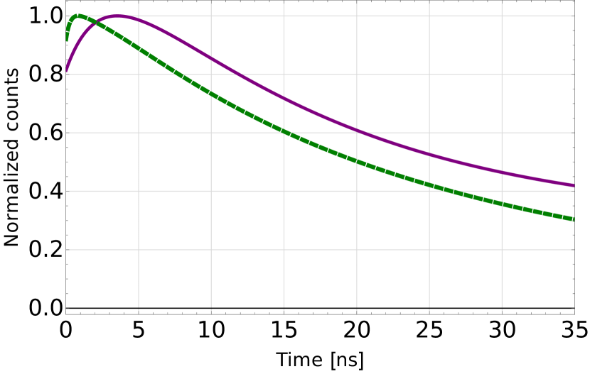
Figure 2: In Figure on the left, a comparison of the fluorescence intensity between Model A (purple solid line) and Model B (green dashed line) for 2 NV centers is presented. Figure on the right is taken from Ref. [1] and presents the simulation results of Model A against experimental data.

The time limit of $35$ ns provides a consistent scale for comparison. Notably, we observe a non-zero initial fluorescence in our results, a phenomenon that is not unexpected as it typically does not originate from zero. While this effect is evident in plot from [1], it may be attributed to experimental data fitting, accounting for laboratory-induced effects. Moreover, our results exhibit no significant deviation at the $35$ ns.

Firstly, it is important to highlight that in Fig. 2, our simulations based on Model A yield slightly different results compared to those obtained through Model B. Though the disparity is currently minor, it may become more pronounced with a larger number of centers. Secondly, we observe notable deviations between the simulated results from Model A and both the experimental data and the declared simulation outcomes reported in Ref.[1], as depicted in Fig. 2 (plot on the right).

Subsequently, we extend our analysis to plot the simulated fluorescence graph for two color centers over a broader time scale ranging from 0 to $100$ ns, as illustrated in Fig. 3. This extended time frame effectively captures long-term discrepancies between Models A and B. Notably, the chart also depicts the asymptotes calculated for both models. In our model, the fluorescence asymptote is 0, reflecting a typical physical outcome. Conversely, in the criticized Model A, fluorescence persists even at infinity.

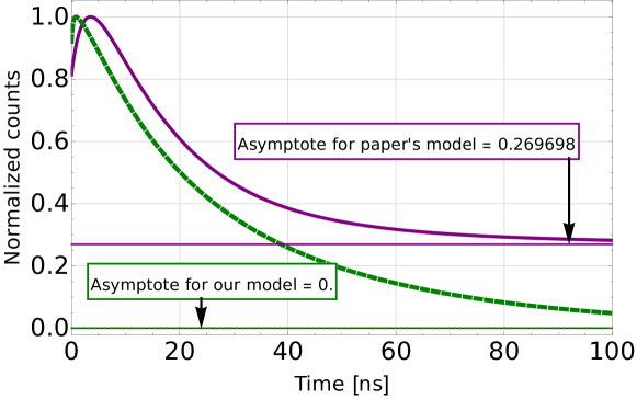
Figure 3: The results of two simulation variants of fluorescence intensity of timespan from $0$ to $100$ ns, for 2 NV centers. The purple solid line represents Model A, while the green dashed line is based on Model B. The asymptotic values for both models are provided.

B.2 N=7

For $N=7$, the intensity plot Fig. 4 obtained from Model A exhibits an sharp decline followed by erratic fluctuations in intensity, culminating in an abrupt rise to a significant value before subsequently decreasing. Upon simulating this scenario for a duration of $100$ ns and beyond, a highly concerning outcome emerges – the photon counts register negative values. To emphasize these anomalous effects, we have incorporated red vertical lines into the simulated charts, marking instances where the fluorescence value reaches $0$. This visual aid facilitates the identification of instances where the charts indicate a change in the sign of fluorescence, which represents an unphysical characteristic. Assuming $N=7$, we also computed asymptotic values for Models A and B. While Model A yields a negative asymptote, which is physically unrealistic, Model B proposed in this paper converges to a zero asymptote, aligning with expected physical behavior.

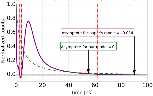
Figure 4: The results of two simulation variants of fluorescence intensity in time from $0$ to $100$ ns, for 7 NV centers. The purple solid line represents Model A, while the green dashed line comes from Model B. Red dashed vertical lines are drawn to indicate where the values of the solid graph change the sign. The asymptotic values calculated for both models are also provided.

B.3 N=10

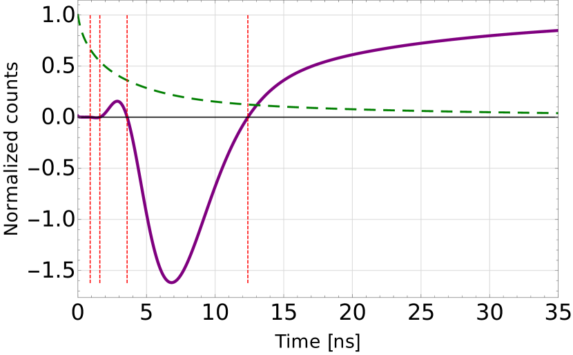
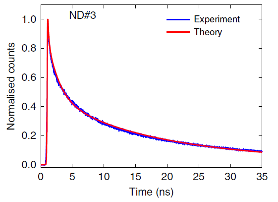
Figure 5: In Figure on the left, a comparison of the fluorescence intensity between Model A (purple solid line) and Model B (green dashed line) for 10 NV centers is presented. Figure on the right is taken from Ref. [1] and presents their simulation results of Model A against experimental data.

Fig. 5 shows the same considerations for $N=10$ and the parameters taken from Tab. 2. Again, our simulations based on Model A starkly contrast with those presented in the referenced paper [1]. Additionally, immediate detection of unphysical effects is evident. Initially, fluorescence nearly reaches zero for several nanoseconds, then sharply increases before declining to strongly negative photon count values. Subsequently, it returns to positive values and stabilizes at an asymptote representing maximum positive intensity. On the other hand, results for Model B do not feature any anomalies (see the green dashed line in Fig. 5).

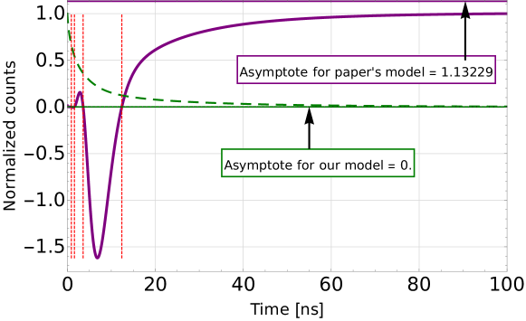
Figure 6: The result of two simulation variants of fluorescence intensity in time from $0$ to $100$ ns, for 10 NV centers. The purple solid line represents Model A, while the green dashed line is based on Model B. Red dashed vertical lines are drawn to indicate where the values of the solid graph change the sign. The asymptotic values calculated for both models are also provided.

Fig. 6 displays a broader time interval, up to $100$ ns, revealing that a constant fluorescence persists even without any external excitation, which cannot be supported by any physical arguments. We observe that within Model B, the fluorescence intensity correctly converges to the asymptotic zero value, indicating that fluorescence vanishes at infinity.

References

- [1] Bradac, C., Johnsson, M., Breugel, M. et al. Room-temperature spontaneous superradiance from single diamond nanocrystals. Nat. Commun. 8, 1205 (2017).
- [2] Bradac, C., Johnsson, M., Breugel, M. et al. Supplementary Information to Room-temperature spontaneous superradiance from single diamond nanocrystals. Nat. Commun. 8, 1205 (2017).
- [3] Gorini, V., Kossakowski, A., and Sudarshan, E. C. G.. Completely Positive Dynamical Semigroups of N Level Systems. J. Math. Phys. 17, 821–825 (1976).
- [4] Lindblad, G. On the generators of quantum dynamical semigroups. Commun. Math. Phys. 48, 119–130 (1976).
- [5] Chruściński, D., and Pascazio, S. A brief history of the GKLS equation. Open Syst. Inf. Dyn. 24, 1740001 (2017).
- [6] Czerwinski A. Dynamics of Open Quantum Systems–Markovian Semigroups and Beyond. Symmetry 14, 1752 (2022).
- [7] Gross, M. and Haroche, S. Superradiance: An essay on the theory of collective spontaneous emission. Phys. Rep. 93, 301–396 (1982).
- [8] Benedict, M., Ermolaev, A., Malyshev, V. et al. Super-radiance: Multiatomic Coherent Emission (Taylor & Francis Group, New York, 1996).