Synchronization of wave-propelled capillary spinners

Abstract

When a millimetric body is placed atop a vibrating liquid bath, the relative motion between the object and interface generates outward propagating waves with an associated momentum flux. Prior work has shown that isolated chiral objects, referred to as spinners, can thus rotate steadily in response to their self-generated wavefield. Here, we consider the case of two co-chiral spinners held at a fixed spacing from one another but otherwise free to interact hydrodynamically through their shared fluid substrate. Two identical spinners are able to synchronize their rotation, with their equilibrium phase difference sensitive to their spacing and initial conditions, and even cease to rotate when the coupling becomes sufficiently strong. Non-identical spinners can also find synchrony provided their intrinsic differences are not too disparate. A hydrodynamic wave model of the spinner interaction is proposed, recovering all salient features of the experiment. In all cases, the spatially periodic nature of the capillary wave coupling is directly reflected in the emergent equilibrium behaviors.

Introduction

Bedridden from a sickness in 1665, Christiaan Huygens observed the coupling of two pendulum clocks Huygens (1895), noticing that the two clocks would begin to oscillate perfectly out of phase when positioned near one another. Realizing that the two oscillators were able to “communicate” via a shared substrate of a heavy beam on which the two clocks were hung, he documented this communication as a “sympathy” the oscillators had towards one another. Over 300 years later, Huygens’ discovery was shown to be one of both “talent and luck”: the weight of the clocks was just right, and the frequencies were just so, such that synchronization could occur in his realization Bennett et al. (2002). Numerous followup studies have continued to interrogate the vast parameter space Oliveira and Melo (2015); Willms, Kitanov, and Langford (2017) and explore general complex phase oscillator networks Martens et al. (2013). An abundance of other artificial and natural systems exhibiting synchronization have since been discovered, such as forests of blinking fireflies Buck and Buck (1966, 1968); Sarfati et al. (2020), human crowds on bridges Fujino et al. (1993); Eckhardt et al. (2007), de-tuned pipe organs Rayleigh (1882); Abel, Ahnert, and Bergweiler (2009), and even the calls of male frogs Aihara et al. (2008). However in many cases, companion mathematical models reproducing such phenomena are purely phenomenological due to the inherent complexity or inaccessibility of the systems. In fact, despite its rich history and apparent simplicity, even the underlying physics of the pendulum system remains an active discussion with much still yet to be learned Goldsztein et al. (2022).

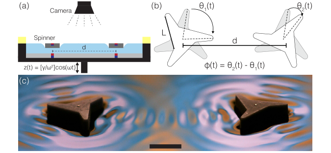
Figure 1: A pair of spinners interact via their mutually generated wavefield. (a) A schematic of the experimental set-up: two spinners are placed on a vertically vibrating bath at a distance $d$ apart, translationally fixed by magnets in and below the spinners. The bath is oscillated vertically with position $z(t)=\gamma/\omega^{2}\cos\left(\omega t\right)$, where $\gamma$ is the acceleration amplitude. (b) The phase difference, $\phi(t)=\theta_{2}(t)-\theta_{1}(t)$ of the spinners, of side length $L=5.7$ mm, is found by tracking $\theta_{1}(t)$ and $\theta_{2}(t)$, comparing the orientation of the spinner at time $t$ (white) to a reference configuration (gray). (c) Oblique perspective of a pair of co-chiral spinners on the surface of a vibrating fluid bath. The self-generated capillary wavefield of the spinner is visualized by the distortions of a reflected color pattern Harris et al. (2017). The shown experiment has parameters $\gamma/g=1.6$, $f=90$ Hz, and $d=28$ mm with a wavelength of $\lambda=3.56$ mm. The scale bar denotes $5$ mm.

With the universality of synchronization in coupled oscillators transcending both animate and inanimate systems, it is perhaps of no surprise that a shared fluid medium, wherein hydrodynamic forces and torques dictate interactions, enables synchronization behaviors at both the micro- Tătulea-Codrean and Lauga (2022); Um et al. (2020); Sabrina et al. (2018); Zhang and Bishop (2023); Riedl et al. (2023); Aubret et al. (2018); Maggi et al. (2015); Di Leonardo et al. (2012); Niedermayer, Eckhardt, and Lenz (2008); Golestanian, Yeomans, and Uchida (2011) and macro-scales Alben (2009); Becker et al. (2015); Saenz et al. (2021); Oza, Ristroph, and Shelley (2019). Of those, a subset focus on the synchronization of microscopic gears often referred to as spinners Aubret et al. (2018); Maggi et al. (2015); Di Leonardo et al. (2012); Sabrina et al. (2018). Here, micrometer-sized spinners are able to communicate via the surrounding fluid at low Reynolds’ number ($\text{Re}=UL/\nu$). This regime is known as the Stokes’ regime, wherein fluid-solid interactions are principally dominated by viscous stresses, with negligible influence of fluid inertia. In general, significantly less is known about propulsion and interactions at intermediate Reynolds numbers, where inertial stresses are comparable to those arising from viscosity Klotsa (2019).

In recent years, the vibrating liquid interface has been used as a tunable and accessible tabletop experimental platform to probe fundamental questions in physics, often by analogy, ranging from topics in quantum mechanics, condensed matter physics, to active matter. Both droplets Couder et al. (2005); Protiere, Boudaoud, and Couder (2006); Pucci (2015); Bush and Oza (2020) and floating solid objects Ho et al. (2023); Barotta et al. (2023); Roh and Gharib (2019); Rhee et al. (2022); Thomson, Barotta, and Harris (2023); Benham, Devauchelle, and Thomson (2024) have been shown to be able to harness energy from mechanical vibrations to produce directed motion via their self-generated wavefield. Multiple interfacial propulsors interact at long-range via the deformed fluid substrate Couchman, Evans, and Bush (2022); Thomson, Couchman, and Bush (2020); Saenz et al. (2021); Nachbin (2020); Ho et al. (2023). Phase synchronization has recently been documented for self-propelling droplets orbiting within small circular corrals that can communicate hydrodynamically via a thin intermediary fluid layer, giving rise to global order in large lattices Saenz et al. (2021). The rich emergent interaction behaviors observed in these interfacial systems have been captured by mathematical modeling derived from first principles Oza, Rosales, and Bush (2013); Oza et al. (2023); Saenz et al. (2021), rather than needing to resort to ad-hoc phenomenological modeling, as is often common for companion dry granular systems where local steric interactions drive both propulsion and interaction.

We herein study the wave-mediated interactions of chiral solid objects atop a vibrating liquid interface. Prior work documented that such capillary spinners steadily rotate via their self-generated wavefield when in isolation Barotta et al. (2023). When two spinners are held at a fixed distance from one another, but otherwise left to rotate freely, we here find that the objects may still spin yet robustly synchronize their phase, with the equilibrium phase angle between the spinners depending sensitively on their spacing and vibration parameters. In particular, the nature of the spinner-spinner coupling is shown to be spatially periodic, a direct consequence of their wave-mediated hydrodynamic interaction. Spinners with different natural rotation rates can either synchronize or exhibit phase drift, depending on the degree of their intrinsic differences and the strength of the coupling. Furthermore, when two spinners are placed sufficiently close to one another, their rotation can be completely arrested via their overwhelming mutual wave interaction. Our principal experimental observations are reproduced by a mathematical model that extends prior work on interacting capillary surfers (polar wave-propelled particles) Oza et al. (2023) to the present case of interacting spinners.

Synchronization of Identical Spinners

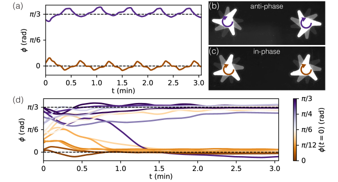
Figure 2: Synchronization of a pair of identical spinners via their mutual wavefield. (a) Time-evolution plots of the phase difference ($\phi=\theta_{2}-\theta_{1}$) between two spinners demonstrates the bistability of in-phase and anti-phase modes for a fixed set of experimental parameters ($f=90$ Hz, $\gamma/g=1.6$, $d=28$ mm). While the phase difference exhibits oscillations, the mean phase difference approaches either $0$ (in-phase) or $\pi/3$ (anti-phase) for different initial conditions. (b-c) Temporal evolution of the anti-phase and in-phase modes, corresponding to the purple and orange curves of (a). (d) Initializing a pair of co-chiral spinners at different initial phase differences ($\phi(t=0)$) leads to either in-phase or anti-phase mode selection over an entire range of initial conditions. The curves in (d) are smoothed over the period of one revolution to highlight the mean phase behavior for 16 independent trials. See Supplementary Video 1 for video of both in-phase and anti-phase synchronization.

A pair of spinners, of side length $L=5.7$ mm, are placed on a liquid (water-glycerol mixture) bath that is vertically vibrated with an acceleration amplitude $\gamma$ and angular frequency $\omega=2\pi f$. The contact line is pinned along the base of the spinner, with its weight supported by buoyancy and surface tension. In order to restrict translational motion, we embed each spinner with a vertically polarized magnet at its center of mass and place a second magnet beneath the bath. This method allows for the center-to-center distance $d$ of a spinner pair to be prescribed for each experiment, allowing for a controlled investigation of the role of spacing on the wave-mediated interaction behavior (Fig. 1(a)). To assess the coordination of the two spinners, we measure their instantaneous phase difference $\phi(t)=\theta_{2}(t)-\theta_{1}(t)$ over time, with $(\theta_{1}(t),\theta_{2}(t))$ being tracked by comparing the current configuration of the spinner at a time $t$ to a reference configuration of the spinner (Fig. 1(b)). Extended details on the experimental setup and details on the tracking and post-processing can be found in Appendices A and B, respectively.

The pair of spinners emit outwardly propagating capillary waves of wavelength $\lambda$ due to the relative motion of the spinner and the liquid bath (Fig. 1(c)). Emission of outwardly propagating capillary surface waves has been shown to be a means of propulsion both for translation Roh and Gharib (2019); Ho et al. (2023); Rhee et al. (2022) and rotation Barotta et al. (2023) along an interface. The excess momentum flux associated with the surface waves yields a net force/torque for translation/rotation whose magnitude can be tuned via the amplitude of the waves Longuet-Higgins and Stewart (1964).

When the three-armed spinner considered here is shaken at driving parameters $\gamma/g=1.6$ and $f=90$ Hz, a stable rotation of a constant angular velocity $\Omega=0.19\pm 0.03$ rad/s is observed. This value is determined by taking the average and standard deviation of the mean rotation speed of 10 different spinners. While this uncertainty reflects variations due to slight manufacturing differences between individuals, the speed of an single spinner exhibits much less variability over time, typically an order of magnitude less than the variation between individuals. When a second spinner is placed in the bath at a center-to-center distance $d=28$ mm, the two spinners continue to spin by the same mechanism, but now also respond to their neighbor’s incident wavefield.

Two example trials with different initial conditions are shown in Fig. 2(a), which displays the evolution of their phase difference over time (Supplementary Video 1). After a brief transient, the spinners rapidly find a constant mean phase angle, $\overline{\phi}$, indicative of synchronization. Oscillations about the mean phase angle can be observed, and are due to both the wave-mediated interactions and extraneous magnetic effects (additional discussion can be found in the Supplemental Material). For this particular spacing and set of driving parameters, the spinners exhibit both in-phase and anti-phase modes with roughly equal probability. The anti-phase Fig. 2(b) and in-phase Fig. 2(c) synchronization appear as $\phi\approx\pi/3$ and $\phi\approx 0$, respectively, given the three-fold symmetry of the spinner.

To more robustly survey the possible equilibrium behaviors at these parameters, a series of 16 independent trials are conducted with different pairs of co-chiral spinners (Fig. 2(d)). Following a transient period, the spinners find either the in-phase or anti-phase mode with roughly equal probabilities. In this plot, the phase difference is smoothed over the rotation period of the spinner to emphasize the mean phase behavior, and highlight the clustering near phase angles of $0$ (in-phase) and $\pi/3$ (anti-phase). Although only three minutes of observation are shown here in order to clearly show the transient period, stable synchronization has been observed for longer trials (see Supplemental Material). Furthermore, if the system is externally perturbed, the spinners will rapidly return to either the in-phase or anti-phase mode, indicative of the system’s bistability for these parameters.

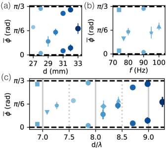
Figure 3: Periodic behavior in the equilibrium mean phase difference ($\overline{\phi}$) for a pair of co-chiral spinners. (a) Mean phase difference as a function of spinner spacing $d$, showing alternating behaviors of bi-stable in/anti-phase and intermediate phase difference. The frequency is fixed at $f=90$ Hz and acceleration amplitude at $\gamma/g=1.6$. (b) Mean phase difference as a function of frequency $f$, showing alternating behaviors of bi-stable in/anti-phase and intermediate phase difference. The spacing is fixed at $d=28$ mm and amplitude of oscillation $a=\gamma/\omega^{2}=0.049$ mm. (c) For both cases, the mean phase difference is plotted as a function of the non-dimensional spinner spacing $d/\lambda$, demonstrating the overall periodicity of the phase behavior on the capillary wavelength. Error bars denote one standard deviation in the equilibrium mean phase difference.

To understand whether this behavior is more generic, experiments are carried out over various values of driving frequency $f$, acceleration amplitude $\gamma$, and spinner spacing $d$ (Fig. 3). We first consider the role of the distance between the spinners. Below the bath, the spacing of the tethering magnets can be adjusted in $1$ mm increments, ranging from $d=27-33$ mm (see Appendix A, Figure 8 for more detail). For each spacing at least 6 trials are conducted. Further trials are conducted for distances admitting bistability of the in-phase and anti-phase modes. The phase difference is tracked over time, and the mean phase difference, $\overline{\phi}$, is recorded by smoothing $\phi$ over a time window equal to one period of rotation and extracting the ending value at the end of the trial. For all trials used, it was ensured that the mean phase angle had become constant. By fixing the driving parameters ($f=90$ Hz, $\gamma/g=1.6$), it can be seen that as the distance increases, the mean phase behavior, $\overline{\phi}$, follows a non-monotonic trend with alternating regions of in-phase and anti-phase bistability (as in Fig. 2) interrupted by spacings that admit only intermediate phase angles, clustered roughly around $\overline{\phi}\approx\pi/6$ (Fig. 3(a)). Mean phase angle for independent trials at a fixed distance were divided into two groups using a k-nearest neighbors (KNN) algorithm. If the difference in the two groups means was greater than $\pi/12$, we classified the system to be in a bistable regime, and reported the results as two separate populations.

Next, the frequency of the bath’s vibration is varied while the spacing is held fixed at $d=28$ mm (Fig. 3(b)). To ensure comparisons could easily be made between experiments at variable frequency, we fix the amplitude of oscillation $a=\gamma/(2\pi f)^{2}=0.049$ mm between experiments to approximately keep the wave amplitude constant between trials. Similar to the distance sweep, as the frequency of oscillation varies, the mean phase difference follows a similar alternating pattern, with the bi-stable in-phase/anti-phase behavior being observed at $74$ Hz in addition to the $90$ Hz case previously showcased in Fig. 2(a,d).

To gain insight as to why similar alternating trends may be arising in both the distance and frequency sweeps, we consider the phase behavior as a function of a dimensionless distance between the two spinners, normalizing the spacing $d$ by the capillary wavelength $\lambda$. Using the dispersion relation for capillary waves Lamb (1924); De Gennes, Brochard-Wyart, and Quéré (2004), we can relate to the wavelength $\lambda$ to the experimental parameters via the capillary wave dispersion relation $\lambda=\left(2\pi\sigma/\rho f^{2}\right)^{\frac{1}{3}}$. By plotting our data from Fig. 3(a) and Fig. 3(b) together with this new abscissa, regions of alternating phase behavior align, and are separated by approximately one wavelength. This periodic interaction behavior directly reflects the wave nature of the hydrodynamic coupling and motivates the development of a dynamical wave-interaction model in what follows.

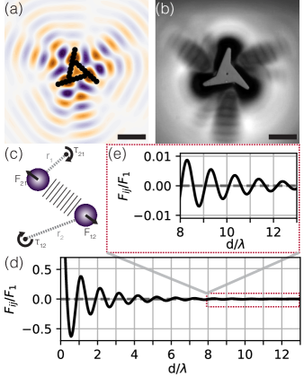
Figure 4: Simulating the wave interactions of capillary spinners. (a) To simulate the wavefield of the spinner, a collection of 24 point wave sources are used to trace out the approximate spinner geometry which recovers the qualitative shape of the experimental wavefield at $f=90$ Hz. (b) Experimental spatial structure of the wavefield can be visualized via a shadowgraph technique shown here at $f=90$ Hz and $\gamma/g=1.6$ demonstrating qualitative agreement with (a). Scales bars for (a,b) denote $5$ mm. See Supplementary Video 2 for video of the isolated spinner self-propelling due to the emitted capillary waves. (c) Each point source acts as both an emitter of waves and also as a location wherein forces, and hence torques, can act from the other spinner. (d) Two wave-emitting point sources exert forces on one another that lead to a non-monotonic, sign-alternating, force profile as a function of their effective distance $d/\lambda$ (Eq. 6). (e) Notably, the force at large effective distances remains oscillatory and finite, allowing for a weak coupling to persist between the spinners. The weak coupling strength ensures that the spinners are still able to effectively rotate under their own self-propulsion for most parameter regimes and large effective distances.

A model of synchronization

In order to further interrogate and isolate the mechanism for synchronization, we develop a simple model of the wave-mediated interactions between two spinners that rotate about fixed centers (Fig. 4). Each spinner is modeled as a collection of wave-emitting point sources ($J=24$ point sources per spinner) that allow us to approximately resolve their relatively complex shape (Fig. 4(a)). As the point source spacing is significantly smaller than the wavelength ($\sim\lambda/5$), introducing additional sources has little effect on the predicted wavefield but increases the computational time of the model. The solution for the wavefield associated with a single oscillatory point forcing on a semi-infinite fluid bath of density $\rho$, viscosity $\nu$, and surface tension $\sigma$ is known from prior work De Corato and Garbin (2018); Oza et al. (2023). The governing equations for the weakly viscous response to a localized parametric point forcing with angular frequency $\omega=2\pi f$ are given by potential flow in the bulk

$$\nabla_{||}^{2}\Phi+\Phi_{zz} =0,$$ (1)

coupled to linearized dynamic and kinematic boundary conditions at the free surface ($z=0$)

$$-\Phi_{t}+\frac{\sigma}{\rho}\nabla_{||}^{2}h+2\nu\nabla_{||}^{2}\Phi+gh+\frac{F_{0}}{\rho}\cos\omega t\delta(\mathbf{x}) =0,$$ (2)

$$\Phi_{z}+2\nu\nabla_{||}^{2}h-h_{t} =0,$$ (3)

where $\Phi$ is the velocity potential, $h$ is the wave height, and $\nabla_{||}=\partial_{xx}+\partial_{yy}$.

The strength of the forcing is given by $F_{0}=\alpha m\gamma$, where $\alpha=0.15$ is an experimentally determined parameter computed by matching the observed wave amplitude for a single isolated spinner ($\gamma/g=1.6$, $f=90$ Hz) to that predicted by the model. Future models could include an additional coupled equation for the vertical response of the floating solid body, as in Benham, Devauchelle, and Thomson (2024), in order to predict this parameter from first principles in the absence of experimental measurements. A more in-depth discussion on $\alpha$ and the manner in which it is determined is provided in Appendix B.

The governing equations can be solved for the wave-profile of a single source $h(r,t)$ Oza et al. (2023). By expressing the height profile as $h(r,t)=\mathbf{Re}\left[H(r)e^{i\omega t}\right]$, the complex amplitude of the wavefield $H(r)$ can be computed as

$$H(r)=\frac{F_{0}}{4\sigma}\sum_{p=1}^{4}\frac{H_{0}(-k_{p}k_{c}r)-Y_{0}(-k_{p}k_{c}r)}{3+4i\epsilon/k_{p}+4\epsilon^{2}k_{p}+\beta/k_{p}^{2}},$$ (4)

where $H_{n}$ and $Y_{n}$ are the $n^{th}$ order Struve function and Bessel function of the second kind, respectively, and the $k_{p}$s are the roots to the polynomial $p(k;\epsilon,\beta)=\epsilon^{2}k^{4}+2ik^{2}+k^{3}+\beta k-1$ as a function of the dimensionless parameters $\epsilon$ and $\beta$. The four parameters appearing in the result for the wavefield profile are

$$k_{c} =\left(\frac{\rho\omega^{2}}{\sigma}\right)^{1/3}, \quad\epsilon =\frac{2\nu k_{c}^{2}}{\omega},$$

$$\quad l_{c} =\sqrt{\frac{\sigma}{\rho g}},\quad \beta =\frac{1}{(k_{c}l_{c})^{2}},$$

and correspond to the wavenumber ($k_{c}$), a reciprocal Reynolds number ($\epsilon$), the capillary length ($l_{c}$), and a wave Bond number ($\beta$). This wavefield has been predicted in prior work, and successfully applied to model the interactions of capillary surfers Oza et al. (2023). The wavefields of each individual point source comprising the spinner are superposed to predict the overall shape of the wavefield (Fig. 4(a)). The predicted wavefield of an individual spinner shows good qualitative agreement with the equivalent experimental visualization (Fig. 4(b)) (Supplementary Video 2), in particular, capturing the pronounced constructive wave “beams” emerging from each wedge. In other systems, complex geometric designs of microgears have prompted similar modeling using a discrete distribution of point sources Di Leonardo et al. (2012). For each spinner, the constituent point sources remain geometrically constrained relative to each another, however the overall structure of 24 sources may rotate about its center of mass in response to various self-induced and external torques described next.

To model the interactions of two spinners, a second spinner is translationally fixed at a center-to-center distance $d$ from the first. Mathematically, we can then describe the system by two second-order ODEs, one for each spinner’s phase $\theta_{n}(t)$ (with $n=1,2$). Each spinner is assumed to be driven by a self-propulsion and wave-interaction term, yielding the governing equations

$$I\ddot{\theta}_{n}=-\frac{I}{{t}_{\nu}}\left(\dot{\theta}_{n}-\Omega_{n}\right)+\sum_{i=1}^{J}\sum_{j=1}^{J}\left[\mathbf{r}_{i}\times\mathbf{F}_{ij}\right]\cdot\hat{\mathbf{z}},$$ (5)

where $J$ is the number of point sources per spinner $(J=24)$, $I$ is the moment of inertia, ${\tau}_{\nu}$ is the viscous timescale, $\Omega_{n}$ is the speed of an isolated spinner, $\mathbf{r}_{i}$ is the position of point source $i$ relative to the center of the spinner, and $\mathbf{F}_{ij}$ is the wave-force between point sources, computed next.

The time-averaged force between two point particles can be found via the equation for the height of the wavefield as in prior work De Corato and Garbin (2018) (Fig. 4(c-e)). We assume that wave force on particle $i$ from the wavefield of particle $j$ is given by $\mathbf{F}_{ij}=\left\langle\left.m_{i}\ddot{z}_{i}\nabla h\left(\mathbf{x}-\mathbf{x}_{j},t\right)\right|_{\mathbf{x}=\mathbf{x}_{i}}\right\rangle$ where $\langle\cdot\rangle$ represents the time average over one oscillation period and $\ddot{z}_{i}=-\alpha\gamma\cos(\omega t)$. Assuming that the two particles oscillate on the fluid interface with the same amplitude and phase, this time-averaged force is given by,

$$\begin{split}\mathbf{F}_{ij}&(r)=\\ &F_{1}\sum_{p=1}^{4}\text{Re}\left[\frac{H_{-1}(-k_{p}k_{c}r)+Y_{1}(-k_{p}k_{c}r)}{1+(4/3)i\epsilon/k_{p}+(4/3)\epsilon^{2}k_{p}+\beta/3k_{p}^{2}}\right]\hat{\mathbf{r}}_{ij},\end{split}$$ (6)

where $F_{1}=\alpha^{2}m_{i}m_{j}\gamma^{2}k_{c}/24\sigma$ and $\hat{\mathbf{r}}_{ij}=\frac{\mathbf{x}_{j}-\mathbf{x}_{i}}{|\mathbf{x}_{j}-\mathbf{x}_{i}|}$.

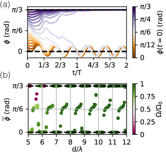
Figure 5: Simulated wave-mediated interactions of a pair of spinners. (a) Like experiment, bi-stability in the mean phase behavior is recovered for parameters corresponding to the experiments in Fig. 2. (b) The dependence of the mean phase angle as a function of effective distance is recovered. Notably, bistable regimes are separated by intermediate zones with phase clustering at $\sim\pi/6$. In addition, a phase locking behavior with the spinners experiencing cessation of rotation is predicted for small effective distances (top left corner in burgundy) wherein the rotation speed $\Omega$ goes to zero following an initial transient.

The two ODEs ($n=1,2$) are coupled via the wave-interaction term. In the absence of this term, the spinner finds an equilibrium steady rotation at speed $\Omega_{n}$, which we extract from experiments on an isolated spinner ($\Omega_{n}=0.19$ rad/s at $90$ Hz and $\gamma/g=1.6$). This value, along with the viscous timescale $(\tau_{\nu}$ = 0.53 s), and the waveheight scaling factor ($\alpha=0.15$) are parameters in our model obtained from experiments on a single spinner. The viscous timescale is found by starting a spinner from constant rotation at $\Omega_{0}$ and shutting off the vibration leading to a slowdown response that is fit to an equation of the form $\Omega(t)=\Omega_{0}e^{-t/\tau_{\nu}}$. Further details on the viscous timescale measurement can be found in Appendix B. Given the relatively large distances $d\gg l_{c}$ between spinners, we omit the capillary attraction forces in the present work, as $F_{c}\sim e^{-d/l_{c}}$ and $d\gg l_{c}\approx 2.4$ mmHo, Pucci, and Harris (2019).

The two-spinner model is solved numerically using parameters corresponding to the experiments shown in Fig. 3. Notably, the simulation is able to recover the observed bi-stability (Fig. 5(a)), with the mean phase difference approaching either 0 (in-phase) or $\pi/3$ (anti-phase) after a brief transient. We additionally explore the role of spinner spacing $d$ in the simulation, with the results of the mean phase summarized in Fig. 5(b). Analogous to the experimental findings in Fig. 3, a distinct periodicity is observed in the mean phase behavior, a direct consequence of the periodicity in the force between two point sources over the characteristic length $\lambda$. For each $d/\lambda$ tested, eight initial conditions $\phi(t=0)$ are chosen for the spinner pairs (uniformly sampled between 0 and $\pi/3$) to ensure that all possible modes of interaction are uncovered.

While the interaction has a clear periodicity, it also has a spatial decay (via both radial spreading and viscous attenuation), that leads to additional trends in the predicted mean rotation speeds of the spinner. For relatively distant spacing, the spinners rotate at a mean speed very close to their isolated free speed, but still manage to synchronize. Their mean rotation speed is reduced as they move closer, with the wave coupling becoming stronger. The simulations further allude to the possibility that in some cases the wave coupling may become sufficiently strong to result in a total stifling of rotation, reminiscent of the “amplitude death” phenomenon for highly coupled phase oscillators Mirollo and Strogatz (1990); Yamaguchi and Shimizu (1984). In this regime, the spinners synchronize their phase to a fixed value but cease to rotate entirely, suggesting that it is possible for the wave-interaction torque to exceed that from self-propulsion. We demonstrate that this behavior is also readily observable in experiment later. A more expansive discussion on the simulation is found in Supplemental Material highlight the robustness of the main phenomena, and trends associated with changes in various model parameters.

Synchronization of Non-Identical Spinners

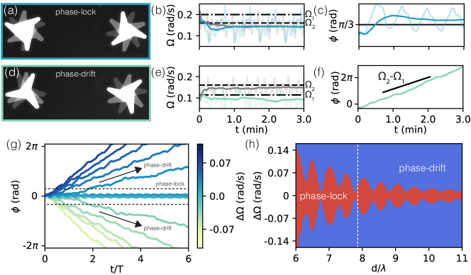
Figure 6: Synchronization of non-identical spinners. With slight modifications to the spinner geometry, the intrinsic angular velocity can be tuned in experiment. (a) When the difference in free speed between two non-identical spinners is small, the pair can synchronize and phase lock. (b) The spinners are able to synchronize. Here, a pair of spinners with free angular velocity $\Omega_{1}=0.20\pm 0.01$ rad/s and $\Omega_{2}=0.16\pm 0.003$ rad/s exhibit anti-phase synchronization (c), with $\overline{\phi}\approx\pi/3$. The smoothed phase difference over one period of rotation is shown opaquely, with the raw data faintly presented in the background. (d) When the difference in angular velocity is too large, the pair instead experiences phase drift and are unable to synchronize. (e) Here, a pair of spinners of free angular velocity $\Omega_{1}=0.114\pm 0.016$ rad/s and $\Omega_{2}=0.16\pm 0.003$ rad/s cannot compromise their intrinsic difference in angular velocity. All experiments are conducted at $f=90$ Hz, $\gamma/g=1.6$, and $d=28$ mm. (f) The phase difference grows at a relatively constant rate roughly equal to the difference in angular velocities, $\Omega_{2}-\Omega_{1}$, indicating that synchronization of the two spinners is not achieved. In (b,e), the gray and colored line denote the angular velocity of the two spinners smoothed over a period of oscillation, with corresponding raw data more faintly in the background. Dashed and dash-dot lines indicate free (isolated) speed for the two spinners. (g) Simulations are able to recover both phase-drift and phase-locking as a function of $\Delta\Omega=\Omega_{2}-\Omega_{1}$ within a small region of $\Delta\Omega=0.02$ rad/s allowing for synchronization to occur at $d/\lambda=7.9$. $\Omega_{1}$ is held fixed at $0.19$ rad/s for all simulations. (h) An expansive sweep over distance $(d/\lambda)$ and $\Delta\Omega$ demonstrate that the admissible $\Delta\Omega$ is a function of the effective distance $(d/\lambda)$ following a functional form reminiscent of the magnitude of the force between two wave-emitting point sources. The dashed white line indicates the value of $d/\lambda$ used in (g). See Supplementary Video 3 for video of both phase-locking and phase-drift for a pair of non-identical spinners.

In the study of phase oscillators, a natural question to consider is whether synchronization remains possible when there exists intrinsic differences between the individuals. Perhaps the most well-known model of such a system is the Kuramoto model Kuramoto (1975, 1984); Acebrón et al. (2005). In this model system, if the difference in intrinsic or natural angular frequency of a pair of oscillators is small, synchronization can still occur, indicated by the phase difference $\phi$ “locking” at a particular value. For larger differences in their intrinsic frequencies, the differences are not able to be reconciled and instead the phase difference “drifts”; increasing or decreasing at a rate approximately equal to the differences in their two natural frequencies $\dot{\phi}\approx\Omega_{2}-\Omega_{1}$.

Although in a real experiment no two spinners are truly identical, to the best of our ability we have demonstrated that synchronization is a robust outcome for two ”identical” spinners over a range of distances and frequencies. This result is similarly recovered in our simulations with identical spinners. However by intentionally introducing intrinsic differences between the two spinners, we can explore the possible analogy with the Kuramoto system. The angular velocity of a spinner in isolation depends sensitively on its geometry Barotta et al. (2023). We here modify the chirality of spinner design to achieve other angular speeds. While holding the overall size of the spinner and wedge opening angle $(\psi=7\pi/9)$ constant, the ratio of the long to short side in each wedge is altered. For our original spinner design, the short to long wedge arm length ratio is given by $q=0.6$. We can continuously vary this ratio, leading to spinners with different intrinsic angular velocities (Fig. 6). The limiting cases of $q=0$ and $1$ correspond to achiral spinners. At $\gamma/g=1.6$, $f=90$ Hz, and $d=28$ mm, we establish a proof of concept for synchronization between non-identical spinners.

When the difference in angular velocity is small (Fig. 6(a-c)) $(\Omega_{1},\Omega_{2})=(0.20\pm 0.01,0.16\pm 0.003)$ rad/s, phase locking is possible, and a mode reminiscent of the anti-phase mode is recovered. Here the original design of short-to-long wedge arm ratio, $q=0.6$, is altered to $q=0.25$ resulting in the speed change. The mean phase difference is not exactly $\pi/3$, presumably due to the difference in natural frequencies. When the difference in angular velocity is larger (Fig. 6(d-f) $(\Omega_{1},\Omega_{2})=(0.114\pm 0.016,0.16\pm 0.003)$ rad/s, phase drift instead occurs. Here, the disparate spinners are unable to compromise their speeds to achieve a synchronized motion brought about by modulating the short to long wedge arm ratio of $0.76$. The time rate of change of the phase difference is roughly constant at a value near the difference in their intrinsic angular velocities ($\overline{\dot{\phi}}\approx 0.05$ rad/s), with fluctuations in the speed and phase difference due to the complex wavefield (Supplementary Video 3). This demonstrates that not only does this system offer a unique platform to study synchronization over an identical population, but it is easily tunable via geometric design to tackle more general notions of synchrony in polydisperse populations.

While our experiments for non-identical pairs offer a proof-of-concept motivating future experimental studies, our simulation allows for a more finely controlled parametric exploration of this behavior. For the purposes of this numerical study, all parameters in the model are fixed to the values corresponding to $\gamma/g=1.6$, $f=90$ Hz, and $d=28$ mm, however the value of the free speed $\Omega_{1}$ is varied with $\Delta\Omega=\Omega_{2}-\Omega_{1}$. In the experimental realization using different spinner geometries, a number of parameters are changing in practice, making a direct comparison more cumbersome. In Fig. 6(g) we show that the simulation is able to recover cases where synchronization is and is not possible depending on the magnitude of $\Delta\Omega$. For these simulations, we initialize all spinner pairs with a phase angle of $\phi(0)=0$ and initial velocities equal to their free speeds in isolation. In particular, we find that there is a band of $\Delta\Omega$ centered around 0 where synchronization (phase locking) is still achieved. In contrast, when $|\Delta\Omega|$ becomes too large, phase drift occurs instead, indicated by the phase difference increasing at a roughly constant rate.

In addition, the breadth of the synchronous band of $\Delta\Omega$ varies as a function of the effective distance (Fig. 6(h)). As the effective distance grows larger, the coupling strength generally is reduced leading to a smaller range of $\Delta\Omega$ admitting synchronization. However, there is also a distinct periodicity in the extent of these regions. The curve separating the phase locking and phase drifting behaviors follows a functional form similar to that of the elemental wave interaction force $|F_{ij}|$ between two point sources. By analogy with the simple Kuramoto model, these results suggest that an appropriately defined effective coupling strength should both decay and oscillate in space. With these various observations as inspiration, future work could attempt to deduce a generalized Kuramoto (GK) model, similar to what is derived in Saenz et al. (2021) for other wave-mediated synchronizing systems.

High Coupling and Amplitude Death

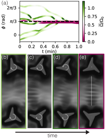
Figure 7: Amplitude death of two spinners in the large coupling limit. (a) When a pair of co-chiral spinners are highly coupled (corresponding to a small effective spacing $d/\lambda$ and large amplitude waves), the amplitude death (zero angular velocity) state of the spinners is observed. Here, the pair of spinners find a preferred orientation causing the pair to stop spinning at $d=28$ mm at $70$ Hz $(d/\lambda=6.6)$. After a crescendo in mean angular speed, the locking state is found, and the pair lock into the stable state shown by the lighter colour in plot wherein $\overline{\Omega}=(|\Omega_{1}|+|\Omega_{2}|)/2$. (b)-(e) is a time sequence demonstrating the route to locking. Notably, in (d), the pair overshoot the equilibrium configuration causing a reversal in the direction of the top spinner before settling into the locking state ($\phi\approx\pi/3$) in (e). (b)-(e) is colour-coded to align with the dynamic rearrangement process as shown in (a) over time. See Supplementary Video 4 for a video of an amplitude death event for a pair of spinners.

For the experimental results presented thus far, dynamic modes of synchronization are achieved over a range of spacing and frequencies, with a mean phase angle between the spinner pair depending sensitively on the effective distance between the two objects. In this regime, the wave-mediated force is sufficiently weak as to not overwhelm the self-propulsion behavior, but still allow for meaningful communication. As suggested by our simulations, we herein demonstrate that further strengthening the coupling can allow for static modes where the resulting speed of each spinner is zero, and the phase is locked indefinitely.

The effective coupling strength can be enhanced by decreasing the relative spacing between the spinners, either by decreasing their dimensional spacing or by decreasing the driving frequency. For pendula, parameter combination that are generally deemed “high coupling” are able to produce amplitude death (alternatively named “beating death”) Bennett et al. (2002); Zou et al. (2021) featuring the complete cessation of oscillation. In our system, this can be interpreted as the halting of spinner rotation. For the parameters studied in Fig. 3, the coexistence of dynamic in-phase and anti-phase was demonstrated. However if the frequency is lowered from 90 to 70 Hz (holding the driving amplitude $\gamma/\omega^{2}$ constant) while keeping the distance fixed at $d=28$ mm ($d/\lambda=6.6$), the two spinners cease rotation, and lock each other in place (Fig. 7(a)). The state is stable for all accelerations tested $\gamma/g=0.9-1.25$, with higher acceleration exploration limited by the Faraday wave threshold $(\gamma_{F}/g\approx 1.3$). We expect that amplitude death is also possible at $90$ Hz, as alluded to by simulation, although in experiment this would require going to smaller effective distances wherein extraneous magnetic interactions between the spinners would become non-negligible.

For all initial conditions tested, the spinners reorient and eventually collapse into a stable static configuration with a phase difference of $\approx\pi/3$. The transient dynamics generally feature an overall slowdown Fig. 7(b-c) of the spinner rotation due to the strong wavefield interaction. However, immediately before the complete cessation of rotation, a large crescendo in the speed is observed Fig. 7(d), where the speed of an individual spinner can momentarily exceed its free speed. Thereafter, the spinners remain locked in place with a standing wave pattern visible between them Fig. 7(e). In this regime, coupling via the wavefield is strong enough to fully overcome the intrinsic self-propulsion (Supplementary Video 4). In some cases, the spinner pair may even overshoot their desired equilibrium phase angle of $\pi/3$ and then reverse rotation direction before reaching the static state.

Discussion and Outlook

We have presented a fluid-mediated system of capillary spinners that self-propel and interact via their mutually generated wavefield. For this study, we have fixed the distance between the objects in order to focus solely on the synchronization of their rotational dynamics. It was found that the equilibrium phase difference between a spinner pair can be tuned as a function of the effective distance, $d/\lambda$, and the system exhibits bi-stable regimes of both in-phase and anti-phase synchronization for a fixed set of experimental parameters. While dynamic regimes were the principal focus of the current study, it was also found that static modes are present with the pair ceasing rotation and locking into a configuration with a fixed phase angle. Finally, experimental tuning of the spinner geometry leads to variations in their intrinsic rotation speeds (analogous to natural frequencies in other oscillator systems) allowing for the system to also be readily applied to study interactions of non-identical oscillators. In general, the interaction behaviors uncovered in this study show distinct signatures of the underlying wave-based coupling.

Given the simplicity and tunability of the experimental setup, questions centered on globally coupled oscillator networks could be considered. In the simplest extension of the current setup, one could untether the spinners by removing the embedded magnets to consider the case where oscillators can both sync and swarm. It has been shown that when analogous polar objects called capillary “surfers” are placed on a vibrating liquid bath, the surfers exhibit spontaneous positional order and swarming behaviors with a variety of stable modes even for the case of a single pair Ho et al. (2023); Oza et al. (2023). In this study, we have demonstrated that surface waves can also lead to rotational synchronization as well which sets up a natural followup of the possibility of simultaneous syncing and swarming. Such oscillators that sync and swarm, known as “swarmalators,” have been a focus of many recent theoretical and numerical studies O’Keeffe, Hong, and Strogatz (2017); O’Keeffe and Bettstetter (2019); O’Keeffe, Ceron, and Petersen (2022) with experimental realizations slowly beginning to emerge Barciś, Barciś, and Bettstetter (2019). The setup presented here is an ideal candidate given that the spinners would be all pairwise coupled to one another via the fluid interface, with the additional benefit that the governing equations of motion are known and amenable to stability analysis Oza et al. (2023). We expect that for an untethered spinner pair, the spinners would synchronize their phase by the wave torque mechanism elucidated here, but also adapt their center-to-center spacing to satisfy the lateral force balance acting on the spinners.

With such a setup in place, moving to large collections of untethered, or tethered, spinners could also be used to study emergent phenomena. On much smaller lengthscales, chiral collections have recently gained attention in both living Tan et al. (2022) and artificial Bililign et al. (2022); Soni et al. (2019); Bricard et al. (2013, 2015) systems with emergent phenomena such as symmetry reversals Workamp et al. (2018), large boundary flows in confinement Yang et al. (2020), lane formation Reeves, Aranson, and Vlahovska (2021), and self-reverting vortices Caprini, Liebchen, and Löwen (2024) being realized. In bouncing droplet systems, which use a similar experimental setup to the one used here, moving to higher collections of interacting drops has already demonstrated various dynamic modes such as soliton formation Thomson, Couchman, and Bush (2020), magnetic order Saenz et al. (2021), and collective motion in droplet rings Couchman and Bush (2020), behaviors that depend sensitively on the lattice structure and number of droplets used. In general, most of the emergent behaviors documented in the bouncing droplet system are isolated to narrow regions of parameter space due to the increased subtleties associated with the droplet’s vertical dynamics and stringent criteria for maintaining non-coalescence behavior. We envision similar types of global phenomena to emerge in the wave-mediated spinner and surfer systems, with the potential for additional effects due to their customizable geometry and their robust engineerable propulsion characteristics.

Such spinner systems have the intrinsic characteristic that their geometry features a form of $n-$fold symmetry. As such, one would expect that the pairing or bonding between a spinner pair to be dictated by their symmetries. Large lattice formation is thus anticipated to be dictated by the shape of the constituent units (spinners) and could result in geometric frustration if a prescribed lattice arrangement is incompatible with the shape of the spinners themselves and their preferred pairwise interaction modes Han et al. (2008); Mellado, Concha, and Mahadevan (2012); Ortiz-Ambriz et al. (2019).

Furthermore, active solids have been a recent topic of interest Baconnier et al. (2022); Fersula, Bredeche, and Dauchot (2024) with applications to odd elasticity, for instance. Flexible, yet steric, connections between active agents exhibit a zoo of behaviors, such as when confined to various lattice structures Baconnier et al. (2022, 2024). Rather than having rigid connections like the aforementioned active solid, the contactless, yet interacting, spinners show promise for being a system where fundamental questions related to odd viscosity might be probed Fruchart, Scheibner, and Vitelli (2023). Given the chiral design of the particle and transverse interactions between adjacent spinners in the plane, the system holds promise to probe further questions in chiral active fluids with a simple tabletop setup Khain et al. (2024); Banerjee et al. (2017); Soni et al. (2019).

Author contributions

J.-W.B., G.P., and D.M.H. designed research; J.-W.B., G.P., and A.H. conducted preliminary experiments; J.-W.B. and E.S. designed final experimental setup; J.-W.B. developed and performed simulations and final experiments; J.-W.B. and D.M.H. analyzed data, developed models, and wrote the paper; all authors performed research, discussed the results, commented on the manuscript and gave final approval for publication, agreeing to each be held accountable for the work performed therein; D.M.H. supervised the project and secured funding.

Appendix A: Experimental Methods

Fabrication of the spinners

The method for fabricating the spinners follows prior work Barotta et al. (2023). The spinners are fabricated using OOMOO 30, a commercially available two-part (Part A and B) silicone rubber compound. Once well-mixed, the mixture is poured into 3D-printed (Formlabs Form 3+, Clear Resin V4) molds designed in Autodesk Fusion 360. A small central extrusion is added to each spinner mold to create a cylindrical pocket for the magnet to be inserted. The CAD file associated with the molds used in the present work are provided with other data presented throughout at the associated digital repository: https://github.com/harrislab-brown/SyncSpinners. Rounded corners at the three tips of the spinner were added to help maintain the pinned contact line along the bottom perimeter throughout the course of the experiments. To pop larger bubbles that formed during the mixing process, and to allow the mixture to make its way into some of the smaller crevices in the mold, the mixture was poured from a height of approximately 1 meter. Excess OOMOO was then scraped off the top of the mold using a straight-edge razor blade. The molds containing the mixture were placed in a vacuum chamber for a total of at least 120 seconds in four 30 second intervals to remove any smaller air bubbles present in the mixture. The surface of the molds were then scraped firmly one final time leaving little-to-no excess compound. The liquid mixture was then cured at room temperature for at least 6 hours, typically overnight. Once cured, the 2 mm-thick spinners were removed from the mold via compressed air. The spinners are then embedded with cylindrical Neodymium 52 magnets (Supermagnetman-Cyl0003-50) of $0.5$ mm height and diameter $0.3$ mm. The cured silicone-rubber compound is naturally hydrophobic. When placed on a water-glycerol bath, the spinners are supported by surface tension and hydrostatic pressure, and remain level with the contact line pinned along the perimeter of their bottom face.

Experimental setup and protocol

A circular fluid bath (depth $H=5.7$ mm and diameter $120$ mm) is mounted atop a rigid aluminum mounting platform and driven vertically using an electrodynamic modal shaker (Modal Shop, Model 2025E). The mounting platform is connected to the shaft of a linear air bearing that interfaces with the shaker via a long flexible stinger, ensuring uniaxial motion at the platform Harris and Bush (2015). For all frequencies and amplitudes explored in the present work, the vertical vibration amplitude was uniform to within 1%. The acceleration amplitude was monitored using two accelerometers (PCB Piezotronics, Model 352C65) mounted diametrically opposed on the driving platform, and a control loop maintained a constant driving amplitude. The entire vibration assembly is mounted on a vibration isolation table (ThorLabs ScienceDesk SDA75120) to minimize any influence of ambient vibrations.

Below the bath, cylindrical Neodymium 42 magnets (K&J Magnetics-D14) of $6.25$ mm height and diameter $1.58$ mm are placed in laser-cut Delrin sheets allowing for the vertical alignment of the magnet-laden spinners (see Fig. 8). This effectively locks the spinners in place with minimal lateral motion of the center of mass of the floating objects and no static friction.

The fluid used in all experiments was a water-glycerol mixture with a density of $\rho=1149.5\pm 0.5$ kg m^-3 measured daily with a density meter (Anton Paar DMA 35A). The water-glycerol mixture has a surface tensionAssociation (1963) of $\sigma=0.067\pm 0.001$ N m^-1 and a dynamic viscosityCheng (2008) of $\mu=0.01\pm 0.0005$ kg m^-1 s^-1.

For each experiment, $64\pm 1$ mL of the water-glycerol solution was measured using a graduated cylinder and poured into the circular bath constructed from laser-cut sheets of acrylic. The working fluid depth ($5.7$ mm) coincides with the thickness of the acrylic sheet to avoid the formation of a border meniscus known to generate small capillary waves that radiate into the bath even in the absence of the spinners Shao et al. (2021). The fluid in the bath was changed at least every thirty minutes to minimize contamination effects. A ring of LEDs was placed $3.8$ cm above the bath to illuminate the spinners (appearing white) against the fluid (appearing black).

Once the bath was filled, each spinner was thoroughly rinsed with deionized water and dried with a dry cleaning wipe (Kimtech Science) before being placed on the bath with a pair of clean tweezers. In the absence of vertical vibration of the bath, the spinner and fluid remained stationary. If the spinner was placed on the bath, and the contact line had any visible imperfections, the spinner was promptly removed and the process restarted.

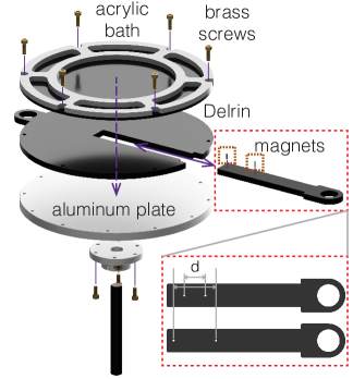
Figure 8: Expanded view of the experimental setup. Exploded view of experimental equipment design for magnetic pinning of interfacial spinners. The top plate is made of two layers of laser cut PMMA (Acrylic) bonded with a Methylene Chloride based solvent (Weld-On 4). The central $120$ mm diameter circular bath is filled with a water-glycerol mixture during experiments. The middle plate is made of laser cut acetal resin (Delrin) with removable inserts for variable magnet spacing (corresponding to spinner spacing $d$). The bottom machined aluminum plate mounts to a vertical shaft constrained by a linear air bearing and is actuated by a modal shaker.

Appendix B: Data Acquisition, Processing, and Parameter Measurement

Tracking rotational motion of the spinners

The spinners are filmed for data acquisition at 3 frames-per-seconds (fps) using an overheard camera (Allied Vision, Mako U-130B) with a macro lens placed 1 meter above and normal to the bath surface. Images were processed in MATLAB: the video frames are run through the geometric transformation estimator imregtform with tformType set to rigid, thus determining both translation and rotation ($\Delta\theta$) of the spinner as compared to a reference image at $t=0$. To obtain the initial phase difference between the spinner pair, the algorithm was additionally run, comparing the two initial frames. Shadowgraph videos were taken at higher frame rates for visual clarity.

Determination of the mean phase angle

The smoothed curves of the phase difference $\phi$ were computed using Matlab’s SmoothMean routine over a trailing number of frames equal to the amount of frames in one rotation of the spinner. For example, if the period of revolution for the spinner was $30$ seconds, the smoothing routine would be done over a trailing window of $90$ frames (corresponding to the 3 frames-per-second recording). The smoothed phase angle $\overline{\phi}$ denotes the mean phase angle over the last period of revolution in the experimental recording or simulations. All trials had reached a steady state for at least one full rotation.

Determination of model parameters

When running simulations of the spinner pair dynamics, experimental parameters for the spinner speed in isolation, viscous timescale, and wave amplitude prefactor are needed. This section describes how those parameters are determined from experiments on single spinners.

The spinner speed in isolation is simply the constant angular velocity achieved by a spinner for a fixed set of driving parameters i.e. $0.19\pm 0.03$ rad/s at $\gamma/g=1.6$ and $f=90$ Hz. A value of $\Omega_{n}=0.19$ rad/s is used in the simulations, unless otherwise stated.

The viscous timescale can also be measured with a single spinner on the bath Fig. 9. Noting that the proposed model for the spinner assumes a linear (viscous) drag, it then follows that when the self-propulsion torque is removed (by dropping the vibration amplitude of the bath to zero) the angular velocity of the response should follow a decaying exponential of the form $\Omega(t)=\Omega_{0}e^{-t/\tau_{\nu}}$, where $\Omega_{0}$ and $\tau_{\nu}$ are the angular velocity right before shutting off the vibration amplitude and and viscous timescale, respectively.

By starting the spinner at different initial angular velocities (achieved by altering the acceleration amplitude at a fixed value of frequency of $f=90$ Hz) 8 trials were conducted and then the measured speed fit to a decaying exponential of the form $\Omega(t)=\Omega_{0}e^{-t/\tau_{\nu}}$ (Fig. 9(a)), with both $\Omega_{0}$ and $\tau_{\nu}$ being determined by the fit. The resulting experimental measurement for the viscous timescale is $0.53\pm 0.03$ s (Fig. 9(b)) across all trials. A value of $\tau_{\nu}=0.53$ s is used for all simulations. We expect the viscous timescale to depend on both geometric design of the spinner, properties of the liquid used, and depth of the bath. We do not expect the viscous timescale to depend on the driving parameters.

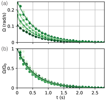
Figure 9: Viscous timescale measurement. (a) A spinner is rotating at a constant speed $\Omega_{0}=\Omega(t=0^{-})$ when the acceleration amplitude is reduced to zero $(\gamma/g=0)$ at $t=0^{+}$ causing the speed to exponentially decay to zero. Markers shown denote experimental measurements of the angular velocity over time, and the best-fit curves for $\Omega(t)=\Omega_{0}e^{-t/\tau_{\nu}}$ are shown for fitting constants $\Omega_{0}$ and $\tau_{\nu}$. (b) By rescaling the $y$ axis by $\Omega_{0}$, the time constant is evidently consistent across trials, taking a value of $\tau_{\nu}=0.53\pm 0.03$ s.

In order to determine a value for the wave amplitude prefactor $\alpha$, the wavefield of a single spinner was measured experimentally using the Fast Checkerboard Demodulation (FCD) method Wildeman (2018) for 90 frames (corresponding to $2.02$ s). The modulus of the wave height at each pixel location was then time-averaged over all frames. A single amplitude value was then determined by averaging the mean wavefield over a small annular region surrounding the spinner ($10\leq R\leq 10.2$ mm). The corresponding wave model for a single spinner was then simulated over one period of oscillation and then averaged in time and over the same annular region as in the experiment. The value of $\alpha$ was then set so that the average value in the annulus was the same between experiment and simulation. The final result of $\alpha=0.15$ was robust, as it was recovered for a range of annuli radii and widths tested. If the annular radius was too large, the experimental measurements are noisy (due to the small wave height) leading to inconsistent results. Similarly if the annular radius was too small, large distortions due to the static meniscus and spurious processing defects associated with the region near the solid body, led to reduced measurement accuracy.

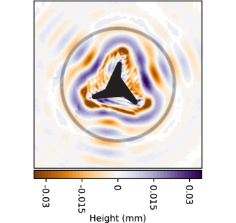
Figure 10: Example wave amplitude measurement. Measured spinner wavefield for a driving parameters of $\gamma/g=1.6$ and $f=90$ Hz. Wave amplitudes are on the order of 10 $\mu$m. The thin gray ring indicates the annular region over which the wave amplitude was averaged in time and space to determine the wave amplitude prefactor $\alpha$ used in simulation.

Data availability

The final experimental data shown for generating Fig. 2,3,6,7 in the study and CAD files for the spinner molds for the shapes used is available at https://github.com/harrislab-brown/SyncSpinners.

Code availability

Code used for simulating a spinner pair is available at https://github.com/harrislab-brown/SyncSpinners.

Competing interests

The authors declare no competing interests.

Additional information

Supplementary information 4 Supplementary Videos and Supplemental Material are available.

References

- Huygens (1895) C. Huygens, “Letters to de sluse,(letters; no. 1333 of 24 february 1665, no. 1335 of 26 february 1665, no. 1345 of 6 march 1665),” Societe Hollandaise Des Sciences, Martinus Nijhoff, La Haye (1895).
- Bennett et al. (2002) M. Bennett, M. F. Schatz, H. Rockwood, and K. Wiesenfeld, “Huygens’s clocks,” Proceedings of the Royal Society of London. Series A: Mathematical, Physical and Engineering Sciences 458, 563–579 (2002).
- Oliveira and Melo (2015) H. M. Oliveira and L. V. Melo, “Huygens synchronization of two clocks,” Scientific Reports 5, 1–12 (2015).
- Willms, Kitanov, and Langford (2017) A. R. Willms, P. M. Kitanov, and W. F. Langford, “Huygens’ clocks revisited,” Royal Society Open Science 4, 170777 (2017).
- Martens et al. (2013) E. A. Martens, S. Thutupalli, A. Fourrière, and O. Hallatschek, “Chimera states in mechanical oscillator networks,” Proceedings of the National Academy of Sciences 110, 10563–10567 (2013).
- Buck and Buck (1966) J. Buck and E. Buck, “Biology of synchronous flashing of fireflies,” Nature 211, 562–564 (1966).
- Buck and Buck (1968) J. Buck and E. Buck, “Mechanism of rhythmic synchronous flashing of fireflies: Fireflies of southeast asia may use anticipatory time-measuring in synchronizing their flashing,” Science 159, 1319–1327 (1968).
- Sarfati et al. (2020) R. Sarfati, J. C. Hayes, É. Sarfati, and O. Peleg, “Spatio-temporal reconstruction of emergent flash synchronization in firefly swarms via stereoscopic 360-degree cameras,” Journal of The Royal Society Interface 17, 20200179 (2020).
- Fujino et al. (1993) Y. Fujino, B. M. Pacheco, S.-I. Nakamura, and P. Warnitchai, “Synchronization of human walking observed during lateral vibration of a congested pedestrian bridge,” Earthquake Engineering & Structural Dynamics 22, 741–758 (1993).
- Eckhardt et al. (2007) B. Eckhardt, E. Ott, S. H. Strogatz, D. M. Abrams, and A. McRobie, “Modeling walker synchronization on the millennium bridge,” Physical Review E 75, 021110 (2007).
- Rayleigh (1882) J. Rayleigh, “On the pitch of organ-pipes,” Phil. Mag 13, 340–347 (1882).
- Abel, Ahnert, and Bergweiler (2009) M. Abel, K. Ahnert, and S. Bergweiler, “Synchronization of sound sources,” Physical Review Letters 103, 114301 (2009).
- Aihara et al. (2008) I. Aihara, H. Kitahata, K. Yoshikawa, and K. Aihara, “Mathematical modeling of frogs’ calling behavior and its possible application to artificial life and robotics,” Artificial Life and Robotics 12, 29–32 (2008).
- Goldsztein et al. (2022) G. H. Goldsztein, L. Q. English, E. Behta, H. Finder, A. N. Nadeau, and S. H. Strogatz, “Coupled metronomes on a moving platform with coulomb friction,” Chaos: An Interdisciplinary Journal of Nonlinear Science 32 (2022).
- Harris et al. (2017) D. M. Harris, J. Quintela, V. Prost, P.-T. Brun, and J. W. M. Bush, “Visualization of hydrodynamic pilot-wave phenomena,” Journal of Visualization 20, 13–15 (2017).
- Tătulea-Codrean and Lauga (2022) M. Tătulea-Codrean and E. Lauga, “Elastohydrodynamic synchronization of rotating bacterial flagella,” Physical Review Letters 128, 208101 (2022).
- Um et al. (2020) E. Um, M. Kim, H. Kim, J. H. Kang, H. A. Stone, and J. Jeong, “Phase synchronization of fluid-fluid interfaces as hydrodynamically coupled oscillators,” Nature Communications 11, 5221 (2020).
- Sabrina et al. (2018) S. Sabrina, M. Tasinkevych, S. Ahmed, A. M. Brooks, M. Olvera de la Cruz, T. E. Mallouk, and K. J. Bishop, “Shape-directed microspinners powered by ultrasound,” ACS Nano 12, 2939–2947 (2018).
- Zhang and Bishop (2023) Z. Zhang and K. J. Bishop, “Synchronization and alignment of model oscillators based on quincke rotation,” Physical Review E 107, 054603 (2023).
- Riedl et al. (2023) M. Riedl, I. Mayer, J. Merrin, M. Sixt, and B. Hof, “Synchronization in collectively moving inanimate and living active matter,” Nature Communications 14, 5633 (2023).
- Aubret et al. (2018) A. Aubret, M. Youssef, S. Sacanna, and J. Palacci, “Targeted assembly and synchronization of self-spinning microgears,” Nature Physics 14, 1114–1118 (2018).
- Maggi et al. (2015) C. Maggi, F. Saglimbeni, M. Dipalo, F. De Angelis, and R. Di Leonardo, “Micromotors with asymmetric shape that efficiently convert light into work by thermocapillary effects,” Nature Communications 6, 1–5 (2015).
- Di Leonardo et al. (2012) R. Di Leonardo, A. Búzás, L. Kelemen, G. Vizsnyiczai, L. Oroszi, and P. Ormos, “Hydrodynamic synchronization of light driven microrotors,” Physical Review Letters 109, 034104 (2012).
- Niedermayer, Eckhardt, and Lenz (2008) T. Niedermayer, B. Eckhardt, and P. Lenz, “Synchronization, phase locking, and metachronal wave formation in ciliary chains,” Chaos: An Interdisciplinary Journal of Nonlinear Science 18 (2008).
- Golestanian, Yeomans, and Uchida (2011) R. Golestanian, J. M. Yeomans, and N. Uchida, “Hydrodynamic synchronization at low reynolds number,” Soft Matter 7, 3074–3082 (2011).
- Alben (2009) S. Alben, “Wake-mediated synchronization and drafting in coupled flags,” Journal of Fluid Mechanics 641, 489–496 (2009).
- Becker et al. (2015) A. D. Becker, H. Masoud, J. W. Newbolt, M. Shelley, and L. Ristroph, “Hydrodynamic schooling of flapping swimmers,” Nature Communications 6, 8514 (2015).
- Saenz et al. (2021) P. J. Saenz, G. Pucci, S. E. Turton, A. Goujon, R. R. Rosales, J. Dunkel, and J. W. M. Bush, “Emergent order in hydrodynamic spin lattices,” Nature 596, 58–62 (2021).
- Oza, Ristroph, and Shelley (2019) A. U. Oza, L. Ristroph, and M. J. Shelley, “Lattices of hydrodynamically interacting flapping swimmers,” Physical Review X 9, 041024 (2019).
- Klotsa (2019) D. Klotsa, “As above, so below, and also in between: mesoscale active matter in fluids,” Soft Matter 15, 8946–8950 (2019).
- Couder et al. (2005) Y. Couder, S. Protiere, E. Fort, and A. Boudaoud, “Walking and orbiting droplets,” Nature 437, 208–208 (2005).
- Protiere, Boudaoud, and Couder (2006) S. Protiere, A. Boudaoud, and Y. Couder, “Particle–wave association on a fluid interface,” Journal of Fluid Mechanics 554, 85–108 (2006).
- Pucci (2015) G. Pucci, “Faraday instability in floating drops out of equilibrium: Motion and self-propulsion from wave radiation stress,” International Journal of Non-Linear Mechanics 75, 107–114 (2015).
- Bush and Oza (2020) J. W. M. Bush and A. U. Oza, “Hydrodynamic quantum analogs,” Reports on Progress in Physics 84, 017001 (2020).
- Ho et al. (2023) I. Ho, G. Pucci, A. U. Oza, and D. M. Harris, “Capillary surfers: Wave-driven particles at a vibrating fluid interface,” Physical Review Fluids 8, L112001 (2023).
- Barotta et al. (2023) J.-W. Barotta, S. J. Thomson, L. F. Alventosa, M. Lewis, and D. M. Harris, “Bidirectional wave-propelled capillary spinners,” Communications Physics 6, 87 (2023).
- Roh and Gharib (2019) C. Roh and M. Gharib, “Honeybees use their wings for water surface locomotion,” Proceedings of the National Academy of Sciences 116, 24446–24451 (2019).
- Rhee et al. (2022) E. Rhee, R. Hunt, S. J. Thomson, and D. M. Harris, “SurferBot: a wave-propelled aquatic vibrobot,” Bioinspiration & Biomimetics 17, 055001 (2022).
- Thomson, Barotta, and Harris (2023) S. J. Thomson, J.-W. Barotta, and D. M. Harris, “Nonequilibrium capillary self-assembly,” arXiv preprint arXiv:2309.01668 (2023).
- Benham, Devauchelle, and Thomson (2024) G. P. Benham, O. Devauchelle, and S. J. Thomson, “On wave-driven propulsion,” Journal of Fluid Mechanics 987, A44 (2024).
- Couchman, Evans, and Bush (2022) M. M. Couchman, D. J. Evans, and J. W. M. Bush, “The stability of a hydrodynamic bravais lattice,” Symmetry 14, 1524 (2022).
- Thomson, Couchman, and Bush (2020) S. J. Thomson, M. M. Couchman, and J. W. M. Bush, “Collective vibrations of confined levitating droplets,” Physical Review Fluids 5, 083601 (2020).
- Nachbin (2020) A. Nachbin, “Kuramoto-like synchronization mediated through faraday surface waves,” Fluids 5, 226 (2020).
- Oza, Rosales, and Bush (2013) A. U. Oza, R. R. Rosales, and J. W. Bush, “A trajectory equation for walking droplets: hydrodynamic pilot-wave theory,” Journal of Fluid Mechanics 737, 552–570 (2013).
- Oza et al. (2023) A. U. Oza, G. Pucci, I. Ho, and D. M. Harris, “Theoretical modeling of capillary surfer interactions on a vibrating fluid bath,” Physical Review Fluids 8, 114001 (2023).
- Longuet-Higgins and Stewart (1964) M. S. Longuet-Higgins and R. Stewart, “Radiation stresses in water waves; a physical discussion, with applications,” in Deep Sea Research and Oceanographic Abstracts, Vol. 11 (Elsevier, 1964) pp. 529–562.
- Lamb (1924) H. Lamb, Hydrodynamics (University Press, 1924).
- De Gennes, Brochard-Wyart, and Quéré (2004) P.-G. De Gennes, F. Brochard-Wyart, and D. Quéré, Capillarity and wetting phenomena: drops, bubbles, pearls, waves, Vol. 315 (Springer, 2004).
- De Corato and Garbin (2018) M. De Corato and V. Garbin, “Capillary interactions between dynamically forced particles adsorbed at a planar interface and on a bubble,” Journal of Fluid Mechanics 847, 71–92 (2018).
- Ho, Pucci, and Harris (2019) I. Ho, G. Pucci, and D. M. Harris, “Direct measurement of capillary attraction between floating disks,” Physical Review Letters 123, 254502 (2019).
- Mirollo and Strogatz (1990) R. E. Mirollo and S. H. Strogatz, “Amplitude death in an array of limit-cycle oscillators,” Journal of Statistical Physics 60, 245–262 (1990).
- Yamaguchi and Shimizu (1984) Y. Yamaguchi and H. Shimizu, “Theory of self-synchronization in the presence of native frequency distribution and external noises,” Physica D: Nonlinear Phenomena 11, 212–226 (1984).
- Kuramoto (1975) Y. Kuramoto, “Self-entrainment of a population of coupled non-linear oscillators,” in International Symposium on Mathematical Problems in Theoretical Physics (Springer, 1975) pp. 420–422.
- Kuramoto (1984) Y. Kuramoto, “Chemical turbulence,” in Chemical Oscillations, Waves, and Turbulence (Springer, 1984) pp. 111–140.
- Acebrón et al. (2005) J. A. Acebrón, L. L. Bonilla, C. J. P. Vicente, F. Ritort, and R. Spigler, “The kuramoto model: A simple paradigm for synchronization phenomena,” Reviews of Modern Physics 77, 137 (2005).
- Zou et al. (2021) W. Zou, D. Senthilkumar, M. Zhan, and J. Kurths, “Quenching, aging, and reviving in coupled dynamical networks,” Physics Reports 931, 1–72 (2021).
- O’Keeffe, Hong, and Strogatz (2017) K. P. O’Keeffe, H. Hong, and S. H. Strogatz, “Oscillators that sync and swarm,” Nature Communications 8, 1–13 (2017).
- O’Keeffe and Bettstetter (2019) K. O’Keeffe and C. Bettstetter, “A review of swarmalators and their potential in bio-inspired computing,” Micro-and Nanotechnology Sensors, Systems, and Applications XI 10982, 383–394 (2019).
- O’Keeffe, Ceron, and Petersen (2022) K. O’Keeffe, S. Ceron, and K. Petersen, “Collective behavior of swarmalators on a ring,” Physical Review E 105, 014211 (2022).
- Barciś, Barciś, and Bettstetter (2019) A. Barciś, M. Barciś, and C. Bettstetter, “Robots that sync and swarm: A proof of concept in ros 2,” in 2019 International Symposium on Multi-Robot and Multi-Agent Systems (MRS) (IEEE, 2019) pp. 98–104.
- Tan et al. (2022) T. H. Tan, A. Mietke, J. Li, Y. Chen, H. Higinbotham, P. J. Foster, S. Gokhale, J. Dunkel, and N. Fakhri, “Odd dynamics of living chiral crystals,” Nature 607, 287–293 (2022).
- Bililign et al. (2022) E. S. Bililign, F. Balboa Usabiaga, Y. A. Ganan, A. Poncet, V. Soni, S. Magkiriadou, M. J. Shelley, D. Bartolo, and W. T. Irvine, “Motile dislocations knead odd crystals into whorls,” Nature Physics 18, 212–218 (2022).
- Soni et al. (2019) V. Soni, E. S. Bililign, S. Magkiriadou, S. Sacanna, D. Bartolo, M. J. Shelley, and W. T. Irvine, “The odd free surface flows of a colloidal chiral fluid,” Nature Physics 15, 1188–1194 (2019).
- Bricard et al. (2013) A. Bricard, J.-B. Caussin, N. Desreumaux, O. Dauchot, and D. Bartolo, “Emergence of macroscopic directed motion in populations of motile colloids,” Nature 503, 95–98 (2013).
- Bricard et al. (2015) A. Bricard, J.-B. Caussin, D. Das, C. Savoie, V. Chikkadi, K. Shitara, O. Chepizhko, F. Peruani, D. Saintillan, and D. Bartolo, “Emergent vortices in populations of colloidal rollers,” Nature Communications 6, 7470 (2015).
- Workamp et al. (2018) M. Workamp, G. Ramirez, K. E. Daniels, and J. A. Dijksman, “Symmetry-reversals in chiral active matter,” Soft Matter 14, 5572–5580 (2018).
- Yang et al. (2020) X. Yang, C. Ren, K. Cheng, and H. Zhang, “Robust boundary flow in chiral active fluid,” Physical Review E 101, 022603 (2020).
- Reeves, Aranson, and Vlahovska (2021) C. J. Reeves, I. S. Aranson, and P. M. Vlahovska, “Emergence of lanes and turbulent-like motion in active spinner fluid,” Communications Physics 4, 92 (2021).
- Caprini, Liebchen, and Löwen (2024) L. Caprini, B. Liebchen, and H. Löwen, “Self-reverting vortices in chiral active matter,” Communications Physics 7, 153 (2024).
- Couchman and Bush (2020) M. M. Couchman and J. W. Bush, “Free rings of bouncing droplets: stability and dynamics,” Journal of Fluid Mechanics 903, A49 (2020).
- Han et al. (2008) Y. Han, Y. Shokef, A. M. Alsayed, P. Yunker, T. C. Lubensky, and A. G. Yodh, “Geometric frustration in buckled colloidal monolayers,” Nature 456, 898–903 (2008).
- Mellado, Concha, and Mahadevan (2012) P. Mellado, A. Concha, and L. Mahadevan, “Macroscopic magnetic frustration,” Physical Review Letters 109, 257203 (2012).
- Ortiz-Ambriz et al. (2019) A. Ortiz-Ambriz, C. Nisoli, C. Reichhardt, C. J. Reichhardt, and P. Tierno, “Colloquium: Ice rule and emergent frustration in particle ice and beyond,” Reviews of Modern Physics 91, 041003 (2019).
- Baconnier et al. (2022) P. Baconnier, D. Shohat, C. H. López, C. Coulais, V. Démery, G. Düring, and O. Dauchot, “Selective and collective actuation in active solids,” Nature Physics 18, 1234–1239 (2022).
- Fersula, Bredeche, and Dauchot (2024) J. Fersula, N. Bredeche, and O. Dauchot, “Self-aligning active agents with inertia and active torque,” Physical Review E 110, 014606 (2024).
- Baconnier et al. (2024) P. Baconnier, O. Dauchot, V. Démery, G. Düring, S. Henkes, C. Huepe, and A. Shee, “Self-aligning polar active matter,” arXiv preprint arXiv:2403.10151 (2024).
- Fruchart, Scheibner, and Vitelli (2023) M. Fruchart, C. Scheibner, and V. Vitelli, “Odd viscosity and odd elasticity,” Annual Review of Condensed Matter Physics 14, 471–510 (2023).
- Khain et al. (2024) T. Khain, M. Fruchart, C. Scheibner, T. A. Witten, and V. Vitelli, “Trading particle shape with fluid symmetry: on the mobility matrix in 3-d chiral fluids,” Journal of Fluid Mechanics 992, A5 (2024).
- Banerjee et al. (2017) D. Banerjee, A. Souslov, A. G. Abanov, and V. Vitelli, “Odd viscosity in chiral active fluids,” Nature Communications 8, 1573 (2017).
- Harris and Bush (2015) D. M. Harris and J. W. M. Bush, “Generating uniaxial vibration with an electrodynamic shaker and external air bearing,” Journal of Sound and Vibration 334, 255–269 (2015).
- Association (1963) G. P. Association, Physical properties of glycerine and its solutions (Glycerine Producers’ Association, 1963).
- Cheng (2008) N.-S. Cheng, “Formula for the viscosity of a glycerol- water mixture,” Industrial & Engineering Chemistry Research 47, 3285–3288 (2008).
- Shao et al. (2021) X. Shao, C. Gabbard, J. Bostwick, and J. Saylor, “On the role of meniscus geometry in capillary wave generation,” Experiments in Fluids 62, 1–4 (2021).
- Wildeman (2018) S. Wildeman, “Real-time quantitative schlieren imaging by fast fourier demodulation of a checkered backdrop,” Experiments in Fluids 59, 97 (2018).