Interference effects in resonant di-Higgs production at
the LHC in the Higgs singlet extension

Abstract

Interference effects are well founded from the quantum mechanical viewpoint and in principle cannot be ignored in realistic studies of New Physics scenarios. In this work, we investigate the size of interference effects between resonant and non-resonant contributions to di-Higgs production in the singlet extension of the Standard Model, where the additional heavy scalar provides a resonant channel. We find these interference contributions to have a non-negligible effect on the cross-sections and differential distributions. In order to allow for a computationally efficient treatment of these effects via reweighting, we introduce a new tool utilising a matrix-element reweighting method: HHReweighter. In addition to the broadly used di-Higgs invariant mass $m_{hh}$, we analyse the sensitivity to the interference terms for other kinematic variables, such as the Higgs boson transverse momentum, and find that these also can be sensitive to interference effects. Furthermore, we provide updates on the latest experimental and theoretical limits on the parameter space of the real singlet extension of the Standard Model Higgs sector.

I Motivation

Higgs pair production is a process of high interest at the LHC because of its sensitivity to the triple-Higgs coupling and therefore to the underlying mechanism of electroweak symmetry breaking and possible modifications of the scalar potential with respect to its prediction in the Standard Model (SM). Thus, a meaningful interpretation of the measured total and differential cross sections of this process requires an accurate theoretical description and simulation. We focus on di-Higgs production stemming from an additional resonance, as e.g. present in models with singlet extensions (see e.g. Refs. Robens:2015gla ; Robens:2016xkb ; Robens:2022cun and references therein). Di-Higgs production has been discussed in great detail in Ref. DiMicco:2019ngk (see also the short summary in Ref. Brigljevic:2024vuv ), where in particular finite widths and interference effects from Refs. Dawson:2015haa ; Dawson:2016ugw ; Lewis:2017dme ; Carena:2018vpt are presented. More recent work on interference effects in di-Higgs production in extended scalar sectors can be found e.g. in Refs. Basler:2019nas ; Heinemeyer:2024hxa .

The assumption of using factorised cross sections has its own merits. One example is the fact that often it is much easier to calculate higher-order corrections to a single $s$-channel production and decay, without taking the full corrections into account. In some cases, these can be $\mathcal{O}\left(100\%\right)$, see e.g. Refs. Ellis:1996mzs ; Campbell:2017hsr , and might easily be more important than a leading order (LO) calculation where the interference effects are correctly described. However, it is not clear a priori that this is the case in all scenarios and realisations of physical models. In particular, for some channels strong relations exist between couplings of new physics particles, e.g. via unitarity relations Gunion:1990kf or other theory constraints. In such cases, it is imperative to include the full matrix elements.

Resonant di-scalar searches are currently investigated by both ATLAS and CMS ATLAS:2024ish ; CMS:2024phk , and correspond to one of the prime channels for testing the scalar sector realised in nature via triple scalar couplings. Therefore, it is of high importance that the correct theoretical description of such processes is consistently applied and up-to-date tools are used in the corresponding simulations. For example, the correct interpretation of results relies on the correct understanding of the simulated process, that might include kinematic effects in differential distributions resulting from irreducible interference terms. First experimental studies showing the possible importance of interference effects in di-Higgs production were presented by the CMS Collaboration in Ref. CMS:2024phk . Similarly, as the finite width of unstable particles is a model prediction, it cannot be set to a value chosen independently of the involved masses and couplings. Note that modifications to the di-Higgs kinematic distributions can also appear in effective field theory interpretations, see e.g. Refs. Carvalho:2015ttv ; Buchalla:2018yce ; Capozi:2019xsi ; Alasfar:2023xpc .

This paper is organised as follows. In Section II, we introduce the real singlet model used for our studies, and briefly discuss general features of width and interference effects in Section III. In Section IV and Section V we describe the tools used to simulate di-Higgs production and present our method for determining regions of the parameter space with sizeable interference effects. We introduce our tool used to model interference effects using matrix-element reweighting in Section VI. This is followed by an investigation of interference effects for several benchmark points with distinct features in Section VII. We summarise our investigations in Section VIII.

II Real singlet extension of the SM

II.1 Summary of the model

In this work, we consider the simplest extension of the Standard Model of particle physics that can provide resonance-enhanced di-Higgs production at colliders. We choose a model that extends the SM electroweak sector by an additional real scalar field that transforms as a singlet under the SM gauge group. This model has been widely discussed in the literature, see e.g. Refs. Schabinger:2005ei ; OConnell:2006rsp ; Patt:2006fw ; Barger:2007im ; Bowen:2007ia ; Robens:2015gla ; Robens:2016xkb ; Huang:2016cjm ; Dawson:2017vgm ; Ilnicka:2018def ; Heinemann:2019trx ; Fuchs:2020cmm ; Robens:2022cun for details.

The most general renormalizable Lagrangian of the SM extended by one real singlet scalar $S$ is given by

$$\mathscr{L}_{s}=\left(D^{\mu}\Phi\right)^{\dagger}D_{\mu}\Phi+\partial^{\mu}S\partial_{\mu}S-V(\Phi,S)\,,$$ (1)

with the scalar potential

$$V(\Phi,S) = -m^{2}\Phi^{\dagger}\Phi-\mu^{2}S^{2}+\left(\begin{array}[]{cc}\Phi^{\dagger}\Phi&S^{2}\end{array}\right)\left(\begin{array}[]{cc}\lambda_{1}&\frac{\lambda_{3}}{2}\\ \frac{\lambda_{3}}{2}&\lambda_{2}\\ \end{array}\right)\left(\begin{array}[]{c}\Phi^{\dagger}\Phi\\ S^{2}\\ \end{array}\right)$$ (7)

$$= -m^{2}\Phi^{\dagger}\Phi-\mu^{2}S^{2}+\lambda_{1}(\Phi^{\dagger}\Phi)^{2}+\lambda_{2}S^{4}+\lambda_{3}\Phi^{\dagger}\Phi S^{2},$$ (8)

where we already imposed a $\mathbb{Z}_{2}$ symmetry that is softly broken by the vacuum expectation value (VEV) of the singlet field $S$.

After minimisation, the model contains in total 5 free parameters in the electroweak sector. A physical choice is Robens:2015gla ; Robens:2016xkb

$$m_{h},\,m_{H},\,v,\,v_{s},\,\sin\alpha,$$ (9)

where the masses of the two physical states are ordered as $m_{h}\,\leq\,m_{H}$, and where $v$ and $v_{s}$ denote the VEVs of the doublet $\Phi$ and singlet $S$, respectively. The mixing angle $\sin\alpha$ corresponds to the angle that rotates the gauge into the mass eigenstates,

$$\begin{pmatrix}h\\ H\end{pmatrix}=\begin{pmatrix}\cos\alpha&-\sin\alpha\\ \sin\alpha&\cos\alpha\end{pmatrix}\begin{pmatrix}\tilde{h}\\ h^{\prime}\end{pmatrix}\,,$$ (10)

where $\Phi=\left(0,(\tilde{h}+v)\right)^{T}/\sqrt{2}$ and $S=\left(h^{\prime}+v_{s}\right)/\sqrt{2}$. Hence, $\sin\alpha\,=\,0$ denotes complete decoupling of the second scalar resonance $S$ from the SM.

In this work, we are interested in interference effects in pair production of the discovered SM-like Higgs boson, $h_{125}$, at a mass of $m_{125}=125\,{\,\rm GeV}$. We therefore identify the lighter state $h$ as $h_{125}$. Similarly, the doublet VEV is fixed to be $v\,\sim\,246\,{\,\rm GeV}$ from electroweak precision measurements. Hence, in total three free parameters remain:

$$m_{H},\,\sin\alpha,\,\tan\beta\,\equiv\,\frac{v}{v_{s}},$$ (11)

which we choose as the independent input parameters in this work.

The trilinear Higgs couplings $\lambda_{ijk}$ (of mass dimension one) play a crucial role in the di-Higgs production processes. They are defined as $V\,\supset\,\sum_{ijk}\,\lambda_{ijk}\,h_{i}\,h_{j}\,h_{k}$, with $\left\{i,j,k\right\}\,\in\,\{1,2\}$ and $h_{1}\,\equiv\,h,\,h_{2}\,\equiv\,H$, where $\lambda_{hhh}$ is expressed in relation to the SM-value as $\kappa_{\lambda_{hhh}}\,\equiv\,\frac{\lambda_{hhh}}{\lambda_{\mathrm{SM}}}$, with $\lambda_{\mathrm{SM}}\,=\,\frac{m_{125}^{2}}{2\,v}$ being the triple scalar coupling in the SM-like case.

The $hhh$ and $hhH$ couplings depend on the model parameters in the following way:

$$\lambda_{hhh} = \lambda_{\mathrm{SM}}\left(\cos^{3}{\alpha}-\tan\beta\sin^{3}{\alpha}\right),$$

$$\lambda_{Hhh} = \lambda_{\mathrm{SM}}\frac{2m_{h}^{2}+m_{H}^{2}}{m_{h}^{2}}\,\frac{\sin\left(2\alpha\right)}{2}\left(\cos{\alpha}+\tan\beta\sin{\alpha}\right).$$ (12)

The total widths of the two scalars are given by

$$\Gamma_{h} = \left(1-\sin^{2}\alpha\right)\Gamma_{\mathrm{SM}},$$

$$\Gamma_{H} = \sin^{2}\alpha\,\Gamma_{\mathrm{SM}}(m_{H})+\frac{\lambda_{Hhh}^{2}\sqrt{1-4m_{h}^{2}/m_{H}^{2}}}{8\pi m_{H}},$$ (13)

where $\Gamma_{\mathrm{SM}}$ is the width computed for a SM-like Higgs boson of a given mass. For small values of $|\sin\alpha|$, these formulas can be approximated using a Taylor expansion around $\sin\alpha=0$:

$$\lambda_{hhh} \approx \lambda_{\mathrm{SM}}\left(1-\frac{3}{2}\sin^{2}\alpha\right),$$

$$\lambda_{Hhh} \approx \lambda_{\mathrm{SM}}\frac{2m_{h}^{2}+m_{H}^{2}}{m_{h}^{2}}\left(\sin\alpha+\tan\beta\,\sin^{2}\alpha\right)\,,$$ (14)

such that we obtain

$$\Gamma_{H} \approx \,\sin^{2}\alpha\,\Gamma_{\mathrm{SM}}(m_{H})+\lambda_{\mathrm{SM}}^{2}\left(\sin^{2}\alpha+2\tan\beta\,\sin^{3}\alpha\right)\left(\frac{2m_{h}^{2}+m_{H}^{2}}{m_{h}^{2}}\right)^{2}\frac{\sqrt{1-4m_{h}^{2}/m_{H}^{2}}}{8\pi m_{H}}.$$

II.2 Constraints on the model

The model discussed here is subject to a large number of theoretical and experimental constraints that have been discussed in detail in the references given above. Here, we focus on the mass region of $m_{H}\,\geq\,2\,m_{h}=250\,{\,\rm GeV}$; in this regime, the most important updates stem from direct searches for di-boson states in the full Run-2 analyses as well as the higher-order contributions to the $W$-boson mass. The latter have first been calculated in Lopez-Val:2014jva , with a recent update in Papaefstathiou:2022oyi . We only require agreement with all constraints on the electroweak scale, which means that the bounds do not include constraints using renormalization group equation running of the couplings.

We include the most up-to-date experimental constraints. We do this by making use of the publicly available tool HiggsTools Bahl:2022igd , that builds on HiggsBounds Bechtle:2008jh ; Bechtle:2011sb ; Bechtle:2013wla ; Bechtle:2020pkv and HiggsSignals Bechtle:2013xfa ; Bechtle:2014ewa ; Bechtle:2020uwn . The allowed parameter space in the $\left(m_{H},\,\sin\alpha\right)$ and $\left(m_{H},\,\tan\beta\right)$ planes is shown in Figure 1. Direct search results stem from $H\rightarrow\,Z\,Z$ CMS:2018amk ; ATLAS:2020tlo , $H\,\rightarrow\,V\,V$ ATLAS:2018sbw ; ATLAS:2020fry , and $H\,\rightarrow\,h\,h$ CMS:2021yci ; ATLAS:2021ifb ; ATLAS:2022xzm .

The parameter scan used here follows the prescription in Refs. Pruna:2013bma ; Robens:2015gla ; Robens:2016xkb ; Ilnicka:2018def . We first applied all possible theoretical and experimental constraints apart from direct search limits and signal strength measurements. This is due to the fact that most of these can be implemented directly in the scan in a straightforward way. The scan then also tests agreement with direct searches and signal strength measurements using the standalone HiggsBounds and HiggsSignals version with results up to 2022. The allowed points are then checked against the most up to date constraints using the most recent version of HiggsTools . The $W$-boson mass was calculated according to Refs. Lopez-Val:2014jva ; Papaefstathiou:2022oyi .

We show the most constraining channel, using the current HiggsTools version, from this last step in Figure 1. This corresponds to an update of the results presented in previous work, as e.g. Robens:2015gla ; Robens:2016xkb ; Ilnicka:2018def ; Robens:2022cun .

Concerning the cross section values used for the determination of the rates, HiggsTools applies a factorised approach, where the production cross sections are obtained by rescaling the respective values given in the Yellow Report 4 of the Higgs working group LHCHiggsCrossSectionWorkingGroup:2016ypw , rescaled by $\sin^{2}\,\alpha$ and $\cos^{2}\alpha$ for $H$ and $h$, respectively. Note that care must be taken to distinguish the validity regimes of the respective calculations: for $m_{H}\,>\,m_{\text{top}}$ the next-to-next-to-LO (NNLO) with next-to-next-to-leading logarithmic resummation value must be taken, as it contains full top quark mass dependence up to next-to-LO order (NLO), while the next-to-NNLO calculation relies on the effective theory and is therefore viable for $m_{H}\,\leq\,m_{\text{top}}$.

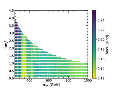
Figure 1: Allowed parameter space in the real singlet extension in the $\left(m_{H},\,\sin\alpha\right)$ (left) and $\left(m_{H},\,\tan\beta\right)$ (right) planes. Maximal values for the third free parameter are shown in colour coding. In addition, on the left side we also display exclusion bounds from the $W$ mass measurement (purple), as well as several resonance searches at the LHC (colour-shaded areas). See text for details.

III Width and interference effects in a nutshell

III.1 Narrow width approximation

In general, from a quantum field theoretical viewpoint, only stable particles can be used as the incoming and outgoing states of the S-matrix (see e.g. Ref. Itzykson:1980rh ), implying that all unstable particles can be treated only as intermediate states (see also the discussion in e.g. Ref. Denner:2019vbn ). In practise, however, it can be advantageous to make use of the narrow width approximation (NWA) pilkuhn1967interactions ; Dicus:1984fu to factorise a more complicated process into the on-shell production of an intermediate particle and its subsequent decay. This way, one can conveniently include higher-order corrections to the production and decay processes. We briefly review the assumptions underlying this approximation.

Let us consider a process $a\,b\,\rightarrow\,S\,\rightarrow\,c\,d$, where we now assume $S$ can be produced and decay resonantly and $a,\,b,\,c,$ and $d$ are stable initial and final state particles, respectively. In the case the $s$-channel is the only contributing diagram, the matrix element can be written via the resummation of the infinite series of self-energy insertions $\Sigma(p^{2})$ between the tree-level propagators $D(p^{2})=i/(p^{2}-m_{S}^{2})$ (see Denner:2019vbn ) as

$$\mathcal{M}_{a\,b\,\rightarrow\,c\,d}\,\,=\,\frac{1}{p^{2}-m_{S,0}^{2}+\hat{\Sigma}(p^{2})}\,\mathcal{F}\sim\,\frac{1}{p^{2}-m_{S}^{2}+i\,\Gamma_{S}\,m_{S}}\,\mathcal{F},$$ (16)

where $p$ denotes the four-momentum in the $s$-channel, $\mathcal{F}$ depends on the four-momenta of the external particles as well as other model parameters, and $m_{S,0},m_{S}$ denote the tree-level mass and physical mass of the scalar, respectively.

In Eq. (16), we used the optical theorem to relate the quantum field theoretical renormalized self-energy, $\hat{\Sigma}$, to the physical total width of $S$, $\Gamma_{S}$, at the pole $p^{2}=m_{S}^{2}$:

$$\text{Im}\hat{\Sigma}\,\left(p^{2}\,=\,m_{S}^{2}\right)\,=\,\Gamma_{S}\,m_{S},$$ (17)

giving rise to the well-known Breit-Wigner propagator in the final step of Eq. (16). For a detailed discussion see e.g. Ref. Fuchs:2016swt . The total width $\Gamma$ corresponds to the sum over all possible partial decay widths.

In the limit of $\Gamma\,\rightarrow\,0$, one obtains

$$\frac{1}{|p^{2}-m^{2}+i\,m\,\Gamma|^{2}}\,\rightarrow\,\frac{\pi}{m\,\Gamma}\,\delta\left(p^{2}-m^{2}\right)$$ (18)

One can also use the Breit-Wigner propagator on the left-hand side of Eq. (18) for finite widths. Further assumptions in the NWA are that the function $\mathcal{F}$ only obtains major contributions around $p^{2}\,\sim\,m^{2}$ and only varies mildly in the region $p^{2}\,\in\,\left[\left(m-\Gamma\right)^{2},\left(m+\Gamma\right)^{2}\right]$. In this case, and making use of phase space factorisation, one obtains the $s$-channel mediated cross section

$$\sigma_{a\,b\,\rightarrow\,c\,d}^{s}\,\simeq\,\sigma_{a\,b\,\rightarrow\,S}\,\times\,\int^{p^{2}_{\text{max}}}_{p^{2}_{\text{min}}}\,\frac{d\,p^{2}}{2\,\pi}\,\frac{2\,m}{|p^{2}-m^{2}+i\,m\,\Gamma|^{2}}\,\times\,\Gamma_{S\,\rightarrow\,c\,d}.$$ (19)

Making use of Eq. (18), the limit $\Gamma\,\rightarrow\,0$ leads to the well-known factorisation into the on-shell production cross section times the branching ratio,

$$\sigma_{a\,b\,\rightarrow\,c\,d}^{s}\,\simeq\,\sigma_{a\,b\,\rightarrow\,S}\,\times\,\underbrace{\frac{\Gamma_{S\,\rightarrow\,c\,d}}{\Gamma}}_{\text{BR}\left(S\,\rightarrow\,c\,d\right)}.$$ (20)

For the case that $\Gamma\,\neq\,0$, one can prove that the formal error of the above approximation is $\mathcal{O}\left(\frac{\Gamma}{m}\right)$. For an introduction as well as discussions of the limitations of the above approximation such as off-shell and threshold effects, the impact of nearby resonances and non-factorisable contributions, see e.g. Refs. Berdine:2007uv ; uhlemann_dipl ; Uhlemann:2008pm ; Cacciapaglia:2009ic ; Fuchs:2015jwa ; Fuchs:2017wkq ; Bagnaschi:2018ofa ; Hoang:2024oeq . See also Ref. Denner:2019vbn for a more general discussion regarding the correct treatment of unstable particles. A generalisation of the NWA to include interference effects in an on-shell approximation was developed in Ref. Fuchs:2014ola .

The result in Eq. (20) highlights the importance of using the physical value of the total width in order to correctly describe the underlying physics. In particular, using the total width as an input parameter $\Gamma_{\text{in}}$, e.g. determined by the detector resolution, in turn leads to arbitrary branching ratios that can easily exceed 1 if $\Gamma\,\equiv\,\Gamma_{\text{in}}\,\leq\,\Gamma_{S\,\rightarrow\,c\,d}$, and therefore unphysical rates. Instead, using a properly calculated total width as a prediction of the model parameters enables a correct physical description.

III.2 Interference effects

Here, we briefly discuss interference effects between resonant and non-resonant contributions to the matrix element of a considered process. In the case of additional contributions to the process $a\,b\,\rightarrow\,c\,d$, namely, diagrams that do not go via the $s$-channel resonance $S$, the total matrix element is given by

$$\mathcal{M}_{\text{tot}}\,=\,\mathcal{M}_{S}\,+\,\mathcal{M}_{\text{rest}},$$ (21)

where $\mathcal{M}_{\text{rest}}$ contains all additional diagrams. For simplicity, let us assume none of these contains an additional resonant channel, i.e. here we do not consider interference between two resonances, but between a resonance and the continuum. The total squared matrix element is thus given by

$$|\mathcal{M}_{\text{tot}}|^{2}\,=\,|\mathcal{M}_{S}|^{2}\,+\,|\mathcal{M}_{\text{rest}}|^{2}\,+\,\underbrace{2\,\text{Re}\left[\mathcal{M}_{S}\,\mathcal{M}^{*}_{\text{rest}}\right]}_{\text{Interference}}.$$ (22)

In case the process is dominated by an on-shell resonance $S$, very often the process is well-described by the first contribution in the above equation. However, it is not a priori clear that this holds for all kinematic variables in the process, including differential distributions or specific regions of phase space. In such cases, all above contributions need to be taken into account. In particular, for processes with electroweak vector bosons in the initial and final state that include scalar $s$-channel contributions, unitarity links these Gunion:1990kf and requires that the full squared matrix element is included for a correct description.

In the following, we will investigate the effect of the interference term in di-Higgs production mediated via an $s$-channel resonance term.

IV Simulation of di-Higgs events

To investigate interference effects between resonant and non-resonant contributions to pair production of SM-like Higgs bosons, we simulate events of gluon fusion di-Higgs production ($gg\to hh$) both at LO and NLO in perturbative quantum chromodynamics (QCD). We perform the LO simulations with the MadGraph5_amc@nlo Alwall:2014hca event generator, using an implementation of the Two Real Singlet Extension of the SM Papaefstathiou:2020lyp with the model file from gitlabandreas . While this model contains three neutral Higgs bosons, we decouple one of these in our implementation. We denote the two non-decoupled scalar fields as $h$ and $H$, where $h$ is identified as the observed Higgs boson with a mass of $m_{h}=125\,{\,\rm GeV}$, and $H$ denotes the additional heavier Higgs boson with a variable mass $m_{H}$. The model leads to contributions to the di-Higgs amplitude from both non-resonant and resonant Feynman diagrams, including interference terms. Among the non-resonant diagrams, the box diagram, $\Box$, (Figure 2, upper-left), is independent of the Higgs trilinear couplings, $\lambda_{i}$, whereas the $s$-channel diagram, $\mathrm{S_{h}}$, depends on the $\lambda_{hhh}$ coupling (Figure 2, upper-right). The resonant $s$-channel contribution, $\mathrm{S_{H}}$, depends on the $\lambda_{Hhh}$ trilinear coupling (Figure 2, bottom).

         

Figure 2: Feynman diagrams of the dominant contributions to di-Higgs production in the SM+singlet model at $pp$ colliders. The upper-left plot displays the so-called box diagram that does not depend Higgs trilinear couplings ($\Box$). The upper-right diagram shows the $s$-channel diagram that depends on $\lambda_{hhh}$ ($\mathrm{S_{h}}$). The resonant contribution to the di-Higgs production due to an additional additional scalar $H$ ($\mathrm{S_{H}}$) is displayed in the lower diagram.

The NLO simulations are performed using the POWHEG 2.0 Nason:2004rx ; Frixione:2007vw ; Alioli:2010xd event generator. Currently there is no POWHEG model that simulates di-Higgs events including both non-resonant and resonant diagrams. Instead we simulate these contributions separately neglecting the interference between resonant and non-resonant diagrams, and in Section VI we will employ a reweighting method to account for the missing interference terms. The non-resonant simulations follow the implementation described in Refs. Heinrich:2017kxx ; Heinrich:2019bkc ; Heinrich:2020ckp . The resonant simulation is performed by generating single $H$ events using the implementation presented in POWHEG Bagnaschi:2011tu , followed by the $H\rightarrow hh$ decay implemented in PYTHIA 8.310 Bierlich:2022pfr .

All samples are generated with the NNPDF3.1 Ball_2017 NNLO parton distribution functions. Parton showering and hadronization are modelled using PYTHIA with the CP5 tune Sirunyan_2020_CP5 .

We also apply a smearing to the outgoing $h$ bosons to study the impact of detector effects on the final distributions. This smearing aims to describe the typical resolution of the four $b$-jet final state. The smearing is performed as follows:

1. The $h$ are first decayed into $b$-quark pairs using PYTHIA.

2. The $\phi$ and $\eta$ direction of the $b$-quarks are smeared independently by shifting the truth-level $\phi$ and $\eta$ on an case-by-case basis by an amount determined from randomly sampling a Gaussian function with a mean of 0 and and an uncertainty of $\sigma_{\phi}=\sigma_{\eta}=0.05$, which is the typical angular resolution for $b$-jets with $p_{\mathrm{T}}\approx 100\,{\,\rm GeV}$ as estimated using simulations of the CMS detector.

3. Finally, the energy/momentum of each $b$-quark is smeared by scaling its 4-vector by $y$, where $y$ is determined by randomly sampling a Gaussian function with a mean of 1 and a width of $\sigma=0.15$. The 15% value is chosen to ensure that the overall resolution on the reconstructed $h$ mass matches the resolution quoted by the CMS Collaboration in Ref. CMS:2019uxx .

We will refer to the smeared $b$-quarks as “$b$-jets” in the following. The $h$ candidates are reconstructed by pairing the $b$-jets. There are three possible combination of pairs, and we choose the combination that minimises $(m_{h_{1}}-125\,{\,\rm GeV})^{2}+(m_{h_{2}}-125\,{\,\rm GeV})^{2}$, where $m_{h_{1}}$ and $m_{h_{2}}$ are the reconstructed masses of the two $h$ candidates. We estimate the di-Higgs invariant mass, $m_{hh}$, following the method in Ref. ATLAS:2022hwc . This method improves the $m_{hh}$ resolution by scaling the four-momenta of each of the reconstructed $h$ such that $m_{h}=125\,{\,\rm GeV}$. Following this method, for signal events with $m_{H}=600\,{\,\rm GeV}$, the $m_{hh}$ resolution is about 6%.

When we study the reconstruction-level distributions in subsequent sections we also apply a loose set of kinematic selections. These selections are chosen to mimic the CMS trigger requirements deployed in Run-3 of the LHC, as described in Ref. CMS-DP-2023-050 . The $b$-jets are required to have $p_{\mathrm{T}}>30\,{\,\rm GeV}$ and $|\eta|<2.5$. The scalar sum of $p_{\mathrm{T}}$ of the four $b$-jets, $\mathrm{H}_{\mathrm{T}}$, is also required to be larger than $280\,{\,\rm GeV}$.

V Numerical investigation of interference effects

In this section, we analyse the parameter dependence of the LO QCD simulations performed with MadGraph5_amc@nlo. In the first part, we discuss in detail different observables and their interference behaviour at two example parameter points. The second part contains a parameter scan, where we are mostly interested in the effect of the interference on the cross-section.

To evaluate the impact of the interference term, we split the diagrams describing the total process $P_{\text{tot}}=pp\rightarrow hh$ into two subprocesses, defined as

• $P_{\mathrm{S_{H}}}=pp\rightarrow H\rightarrow hh$,

• $P_{\text{woH}}=pp\rightarrow hh$ without $H$.

To generate the $P_{\text{woH}}$ subprocesses, which include the $\Box$ and $\mathrm{S_{h}}$ diagrams as shown in Figure 2, we set the coupling constant $\lambda_{Hhh}$ to zero in the simulation. For the widths of the Higgs bosons $H$ and $h$, we use an estimated tree-level total width, consisting of the partial widths for $h\rightarrow VV^{\left(*\right)}$, $h\rightarrow ff$, and $H\rightarrow hh$ and an effective $h\rightarrow\gamma\gamma$ partial width. As the current model file does not include the gluonic decay mode automatically, we also sum this decay width by hand, where we use the full top quark mass dependence and perform the calculation at LO. All partial widths were calculated with MadGraph5_amc@nlo. Some example values are shown in Table 1.

Higgs mass $m_{H}$ [GeV]	260	320	380	440	500	560	620	680	740	800
$\Gamma_{H\rightarrow gg}^{\text{SM}}$ [MeV]	2.111	4.895	13.55	21.64	27.64	32.24	35.87	38.79	41.17	43.14
$\Gamma_{H}$ [GeV]	0.043	0.111	0.214	0.370	0.570	0.817	1.115	1.472	1.891	2.380

Table 1: For a Higgs mass as given in the first row, the second row shows the $H$ decay widths into $gg$ as in the SM ($\Gamma_{H\rightarrow gg}^{\text{SM}}$) for that given mass. The third row shows the total decay width of $H$, calculated as the sum of all partial widths (all decays apart from $H\to gg$ are automatically taken into account by MadGraph5_amc@nlo and $\Gamma_{H\rightarrow gg}=\sin^{2}\alpha\,\Gamma_{H\rightarrow gg}^{\text{SM}}$ is added), evaluated at the example parameter point of $\sin\alpha=0.08$ and $\tan\beta=1$. The maximal branching ratio into the digluon final state for the points in the table is about 0.048 $\%$.

V.1 Illustration of interference Effects

For illustrative purposes, we show the results for two parameter points, namely the points $m_{H}=300\,{\,\rm GeV}$, $\sin\alpha=0.17$, and $\tan\beta=3.3$; and $m_{H}=600\,{\,\rm GeV}$, $\sin\alpha=0.17$, and $\tan\beta=1.6$. For these points, we simulated $10^{6}$ events for each subprocess, $P_{\text{tot}}$, $P_{\mathrm{S_{H}}}$ and $P_{\text{woH}}$. We investigate the interference effects for different observables directly by evaluating the difference between the coherent sum $P_{\text{tot}}$ of all contributions to $gg\to hh$ and the incoherent sum $P_{\mathrm{S_{H}}}+P_{\text{woH}}$. In particular, we analyse the $m_{hh}$, $p_{\mathrm{T}}$, and $\Delta\phi_{hh}$ distributions, where $\Delta\phi_{hh}$ is the angle between the final state Higgs bosons. Here, $p_{\mathrm{T}}$ is shown for both final state Higgs bosons. While the behaviour of the di-Higgs invariant mass is well known, and the corresponding interference effects have been discussed in detail in the literature (see e.g. Ref. DiMicco:2019ngk and references therein), other variables have not been investigated yet. However, all of these can in principle serve as input for both cut-based as well as machine learning based analyses. Therefore, it is imminent to equally be aware of interference effects in as many as possible differential distributions.

As we will discuss in the following, $m_{hh}$ and $p_{\mathrm{T}}$ show interesting interference effects, as can be seen in Figure 3, which shows the number of total events expected using full Run-2 luminosity $\int\mathcal{L}\,=\,139\,{\rm fb}^{-1}$. In contrast, $\Delta\phi_{hh}$ is not significantly affected for these parameters points, and we chose to defer the corresponding discussion to Appendix A. We observe the well-known peak-dip structure around $m_{hh}\,\sim\,m_{H}$, that has already been discussed in the literature. For $m_{hh}$ slightly larger than the mass of the heavy scalar, there is a negative interference that leads to a smaller number of events than expected from incoherently adding the different distributions. A similar effect appears for $m_{hh}$ slightly below $m_{H}$, although the interference effect has a different sign. These are therefore regions in the $m_{hh}$ distributions where interference effects can become important. The interference behaves similarly for the $p_{\mathrm{T}}$ distributions, with positive interference for $p_{\mathrm{T}}$ lower than the peak and negative interference for $p_{\mathrm{T}}$ higher than the peak.

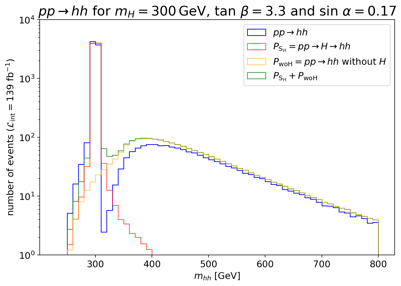
(a)

(b)

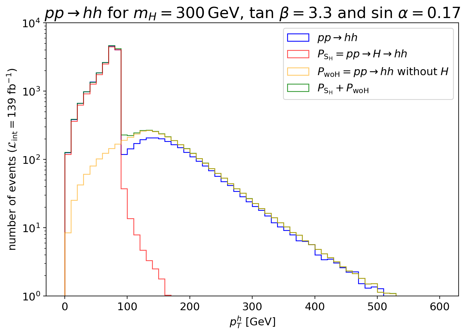
(c)

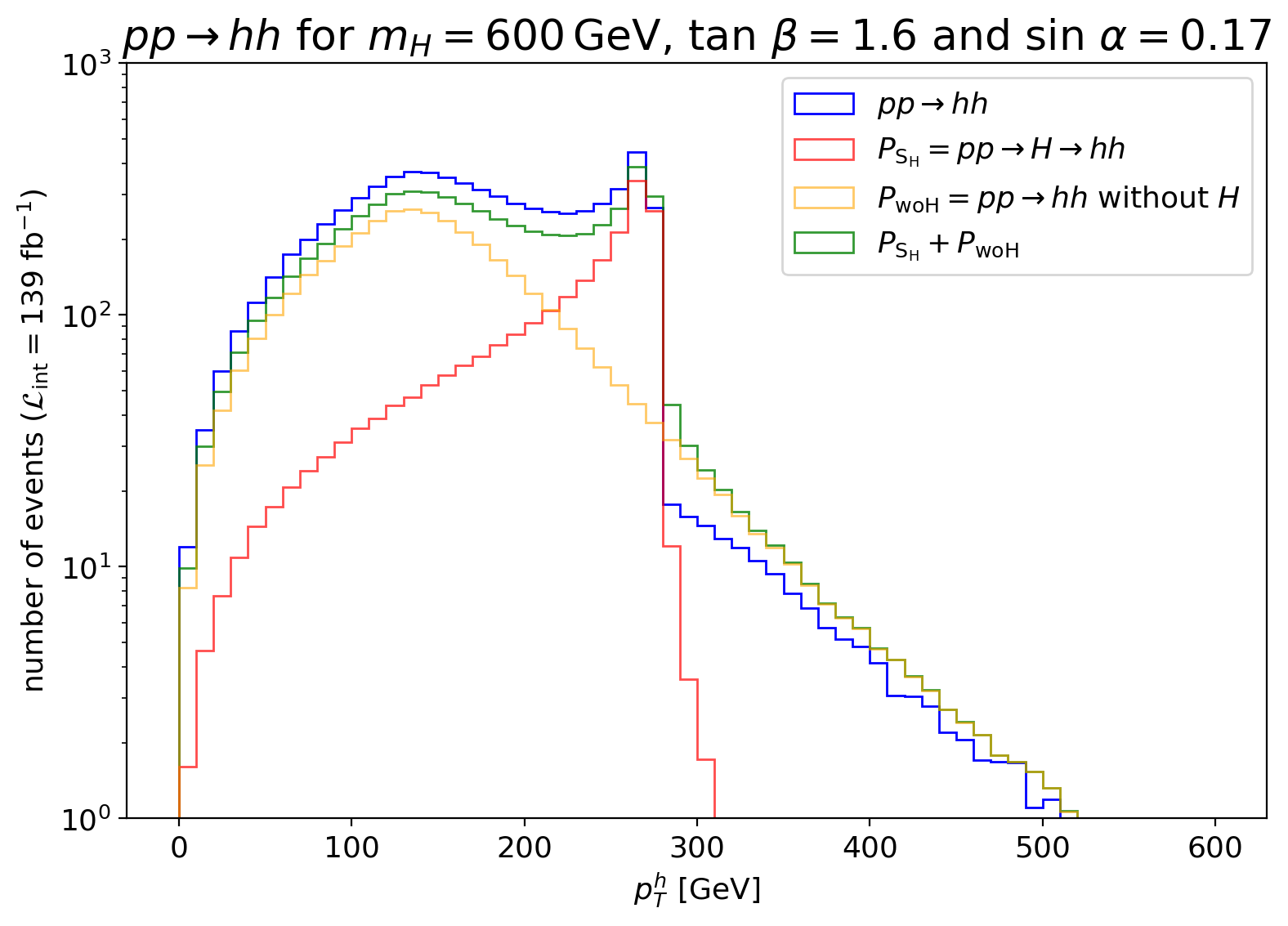
(d)

Figure 3: The upper plots show the invariant mass $m_{hh}$ and the lower plots show the transversal momenta $p_{\mathrm{T}}$ of both final state Higgs bosons for the two parameter points. The blue line corresponds to $N_{\text{tot}}$, the red line corresponds to $N_{\mathrm{S_{H}}}$, the orange line corresponds to $N_{\text{woH}}$ and the green line is the sum $N_{\mathrm{S_{H}}}+N_{\text{woH}}$ neglecting interference effects. The event numbers $N_{i}$ corresponding to process $P_{i}$ were simulated assuming full Run-2 luminosity. The bin size is $10\,{\,\rm GeV}$.

Another important question is whether these effects are statistically significant. In Figure 4, we therefore show the relative difference for the event numbers for the full Run-2 luminosity. As a simple estimate, we only take statistical errors into account. We see that the interference effects are non-negligible over large regions of parameter space, and exceed the statistical uncertainty estimate we applied.

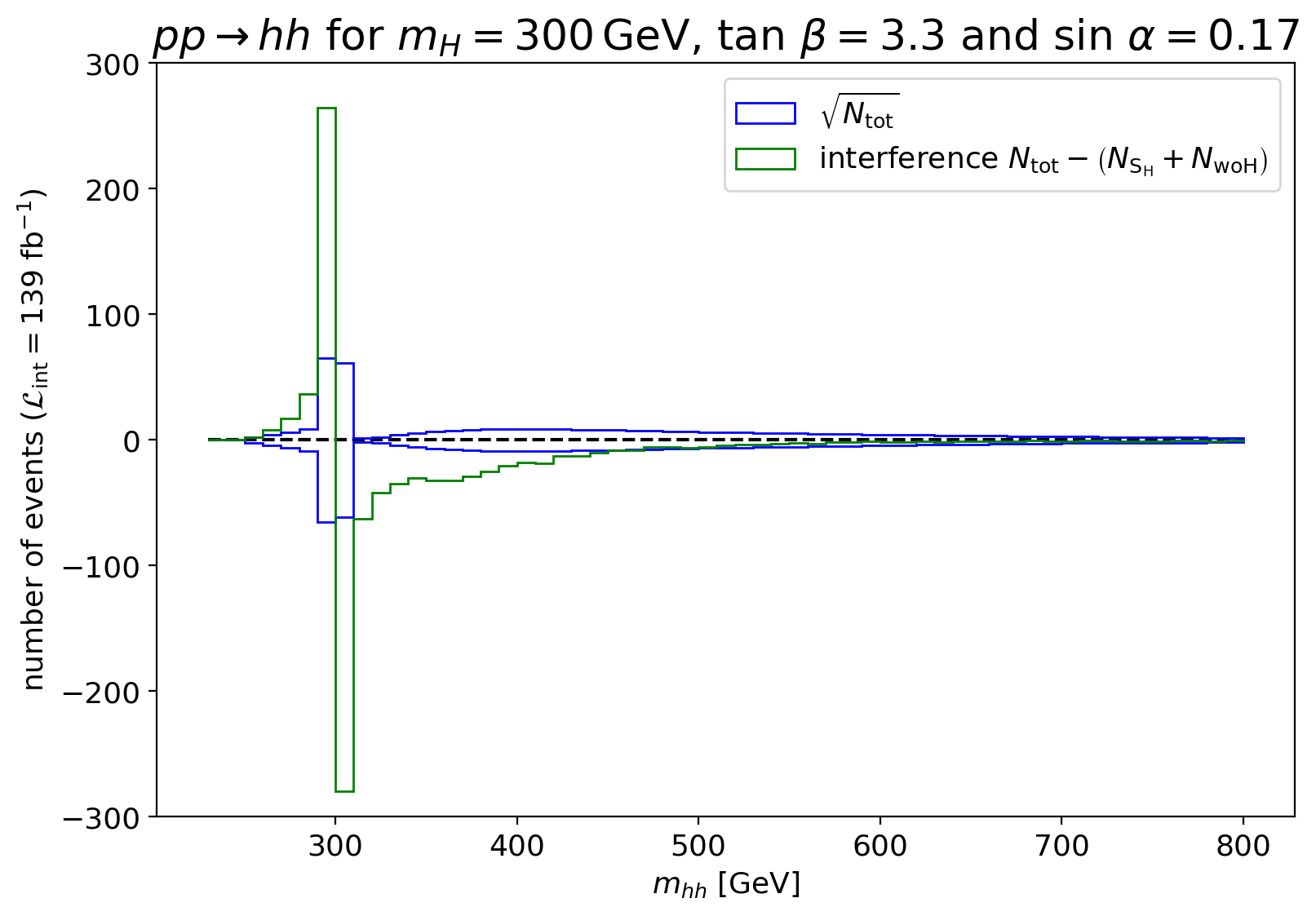
(a)

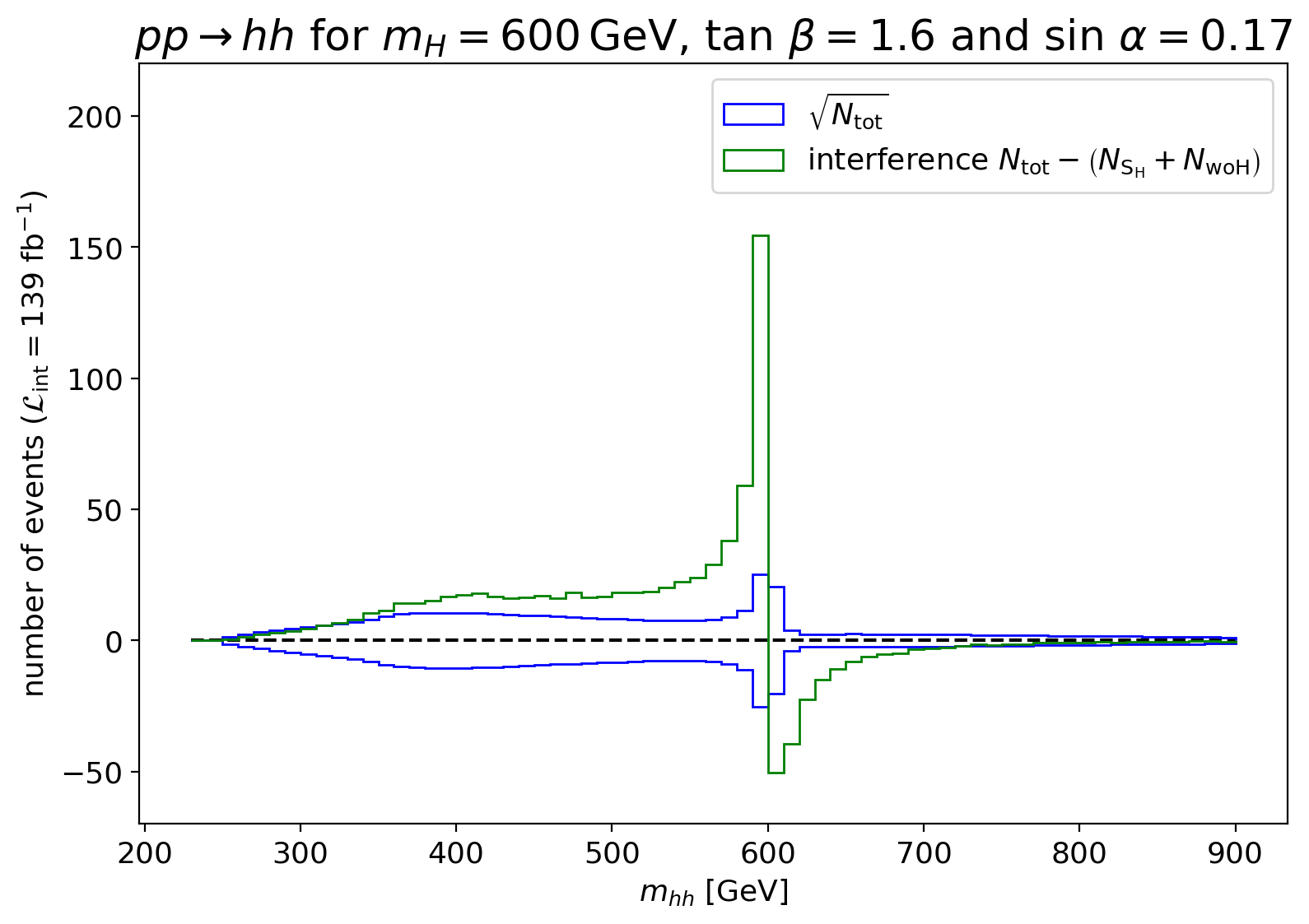
(b)

(c)

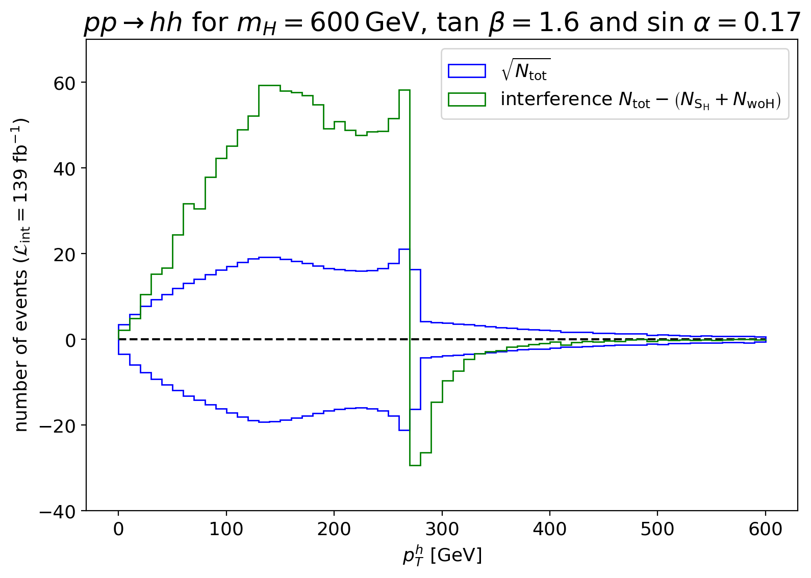
(d)

Figure 4: These plots show the interference calculated from the difference between the blue line and the green line seen in Figure 3 as the green line and a statistical error calculated as the $\sqrt{N_{\text{tot}}}$ of the $P_{\text{tot}}$ process assuming full Run-2 luminosity. The upper plots show this for the invariant mass $m_{hh}$ and the lower plots show this for the transversal momentum $p_{\mathrm{T}}$ for the two parameter points.

V.2 Parameter scan

To investigate the effects of interference between the resonant and non-resonant diagrams, we examine the cross-section corresponding to the interference term for a broad range of parameters. For this purpose, we perform a parameter scan for a range of the relevant parameters in the parameter volume of $[260\,{\,\rm GeV},800\,{\,\rm GeV}]\times[-0.24,0.24]\times[0.5,4.0]$ of the $\{{m_{H},\sin\alpha,\tan\beta\}}$ space where we scan $m_{H}$ in steps of $60$ GeV, $\sin\alpha$ is steps of $0.08$ and $\tan\beta$ in steps of $0.5$. The resulting parameter points are displayed in Table 2. We omitted the points with $\sin\alpha=0$ as they represent the SM case where the second Higgs decouples.

parameter					values
$m_{H}$ [GeV]	260	320	380	440	500	560	620	680	740	800
$\sin\alpha$			-0.24	-0.16	-0.08	0.08	0.16	0.24
$\tan\beta$		0.5	1.0	1.5	2.0	2.5	3.0	3.5	4.0

Table 2: Parameters used in the interference scan.

We then investigated the absolute and the relative interference, defined as

$$\left(\Delta\sigma\right)_{\text{abs}} =\sigma_{P_{\text{tot}}}-\sigma_{P_{\mathrm{S_{H}}}}-\sigma_{P_{\text{woH}}}~{}\text{and}$$ (23)

$$\left(\Delta\sigma\right)_{\text{rel}} =\frac{\left(\Delta\sigma\right)_{\text{abs}}}{\sigma_{P_{\text{tot}}}},$$ (24)

respectively. In Figures 5a and  5b, we display the absolute and relative interference, where we mark all points in the volume which are excluded by the constraints in Section II.1 as triangles, while allowed points are represented by circles. We observe that the interference is largest for high values of $\sin\alpha$, while the size of the interference decreases for small values of $m_{H}$ and/or $\sin\alpha$. Furthermore, the absolute values of $\left(\Delta\sigma\right)_{\text{rel}}$ are larger for positive than for negative interference, reaching 12.6 $\%$ and -4.6 $\%$ for the allowed points, respectively. We checked that we generated sufficient events such that the interference terms are more significant than the statistical uncertainty at the respective parameter point.

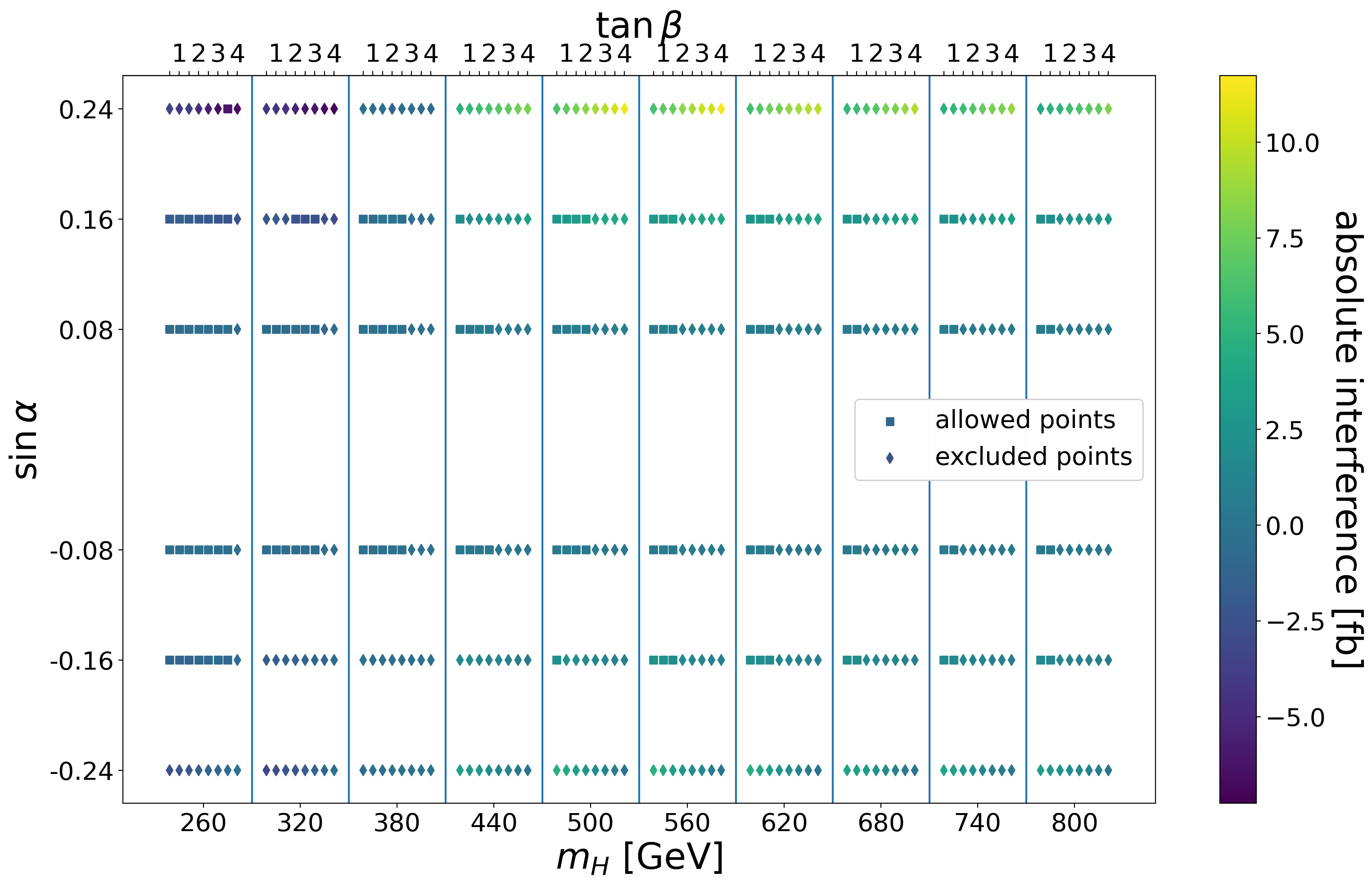
(a) $\left(\Delta\sigma\right)_{\text{abs}}$

(b) $\left(\Delta\sigma\right)_{\text{rel}}$

Figure 5: The different bins on the x-axis show the investigated values of $m_{H}$. The points inside the bins are ordered by the corresponding $\tan\beta$ values from left to right. The y-axis shows $\sin\alpha$, where the SM case of $\sin\alpha=0$ is omitted. Circles represent allowed points and triangles represent the points that do not pass the scan constraints described in Section II. The maximal relative interference for allowed points is around $13\%$. The colours of the points indicate the size of $\left(\Delta\sigma\right)_{\text{abs}}$ and $\left(\Delta\sigma\right)_{\text{rel}}$ for the left and right plots, respectively.

We investigated the interference effects for events with invariant mass $m_{hh}$ above or below $m_{H}$. For this we used the pylhe pylhe python package to divide our generated events into those with higher and those with lower invariant mass than the respective $m_{H}$. Accordingly, we split the cross-sections into the lower invariant mass range, $\left(\Delta\sigma\right)_{\text{abs}}^{<}$, and for the higher invariant mass range, $\left(\Delta\sigma\right)_{\text{abs}}^{>}$, respectively, as well as their absolute sum

$$\left(\Delta\sigma\right)_{\text{abs}}^{\sum}\,\equiv\,\left|\left(\Delta\sigma\right)_{\text{abs}}^{<}\right|+\left|\left(\Delta\sigma\right)_{\text{abs}}^{>}\right|$$ (25)

and the corresponding relative interferences $\left(\Delta\sigma\right)_{\text{rel}}^{<}$, $\left(\Delta\sigma\right)_{\text{rel}}^{>}$ and $\left(\Delta\sigma\right)_{\text{rel}}^{\sum}$, defined accordingly by normalisation to the total cross-section over the whole mass range, equivalent to Eq. (24). The results are displayed in Figure 6. As shown in Figures 3a and especially 3b, the interference seems to have a positive value for $m_{hh}<m_{H}$ and a negative value for $m_{hh}>m_{H}$. Therefore, although the total interference integrated over the whole mass range might be small in some scenarios, effects in differential distributions could still be large. We therefore also provide the corresponding information on the different mass regions discussed above as well as the absolute value of deviations between naive summing of the different contributions and the total process including interference. Figure 6a shows that a higher positive mixing angle enhances both $\left(\Delta\sigma\right)_{\text{abs}}^{<}$ and $\left(\Delta\sigma\right)_{\text{rel}}^{<}$, see Figure 6b. Furthermore, Figure 6c shows that $\left(\Delta\sigma\right)_{\text{abs}}^{>}$ has the largest negative values for large mixing angles in the $m_{H}$ region around $380\,{\,\rm GeV}$, see also Figure 6d. Figure 6e and especially Figure 6f show that some points, which appeared to have negligible interference based on the total cross-sections ($\left(\Delta\sigma\right)_{\text{abs}}$ and $\left(\Delta\sigma\right)_{\text{rel}}$) displayed in Figures 5a and 5b, actually experience two interference effects of opposite sign, which partially cancel when the total cross-section is computed. In Section VII.2 we will introduce benchmark (BM) points that exhibit this feature (benchmarks BM2 and BM3).

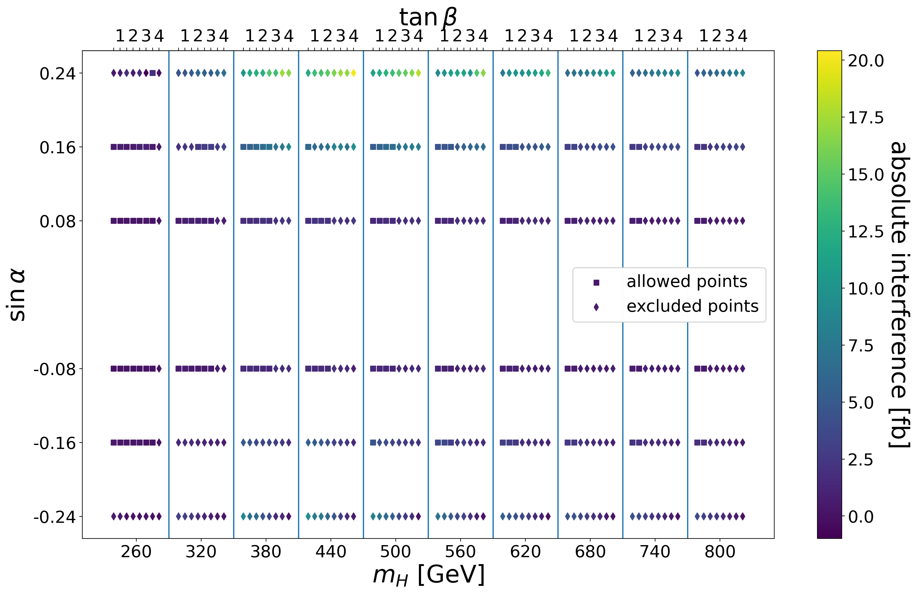
(a) The total interference $\left(\Delta\sigma\right)_{\text{abs}}^{<}$ for $m_{hh}<m_{H}$.

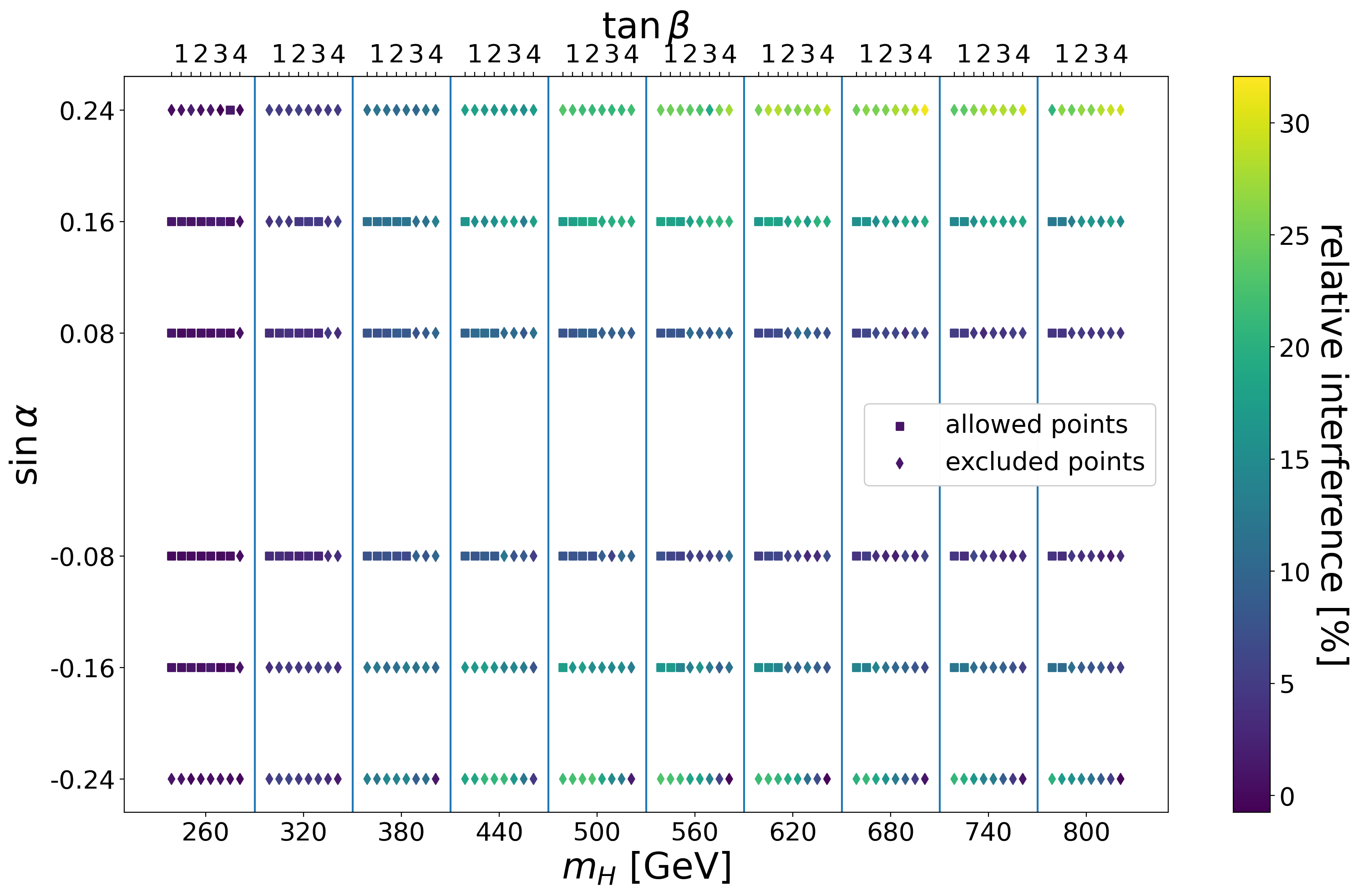
(b) The relative interference $\left(\Delta\sigma\right)_{\text{rel}}^{<}$ for $m_{hh}<m_{H}$.

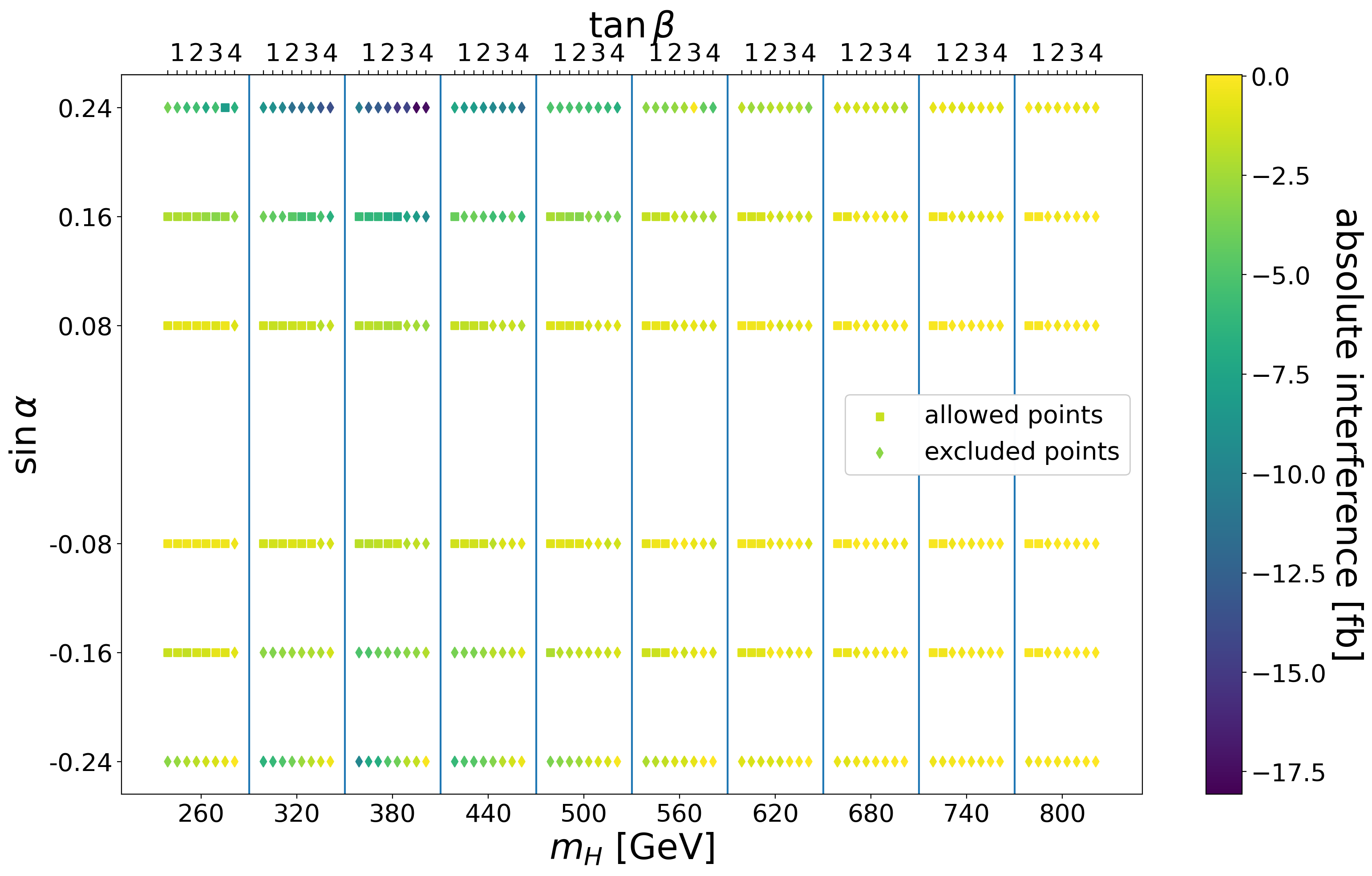
(c) The total interference $\left(\Delta\sigma\right)_{\text{abs}}^{>}$ for $m_{hh}>m_{H}$.

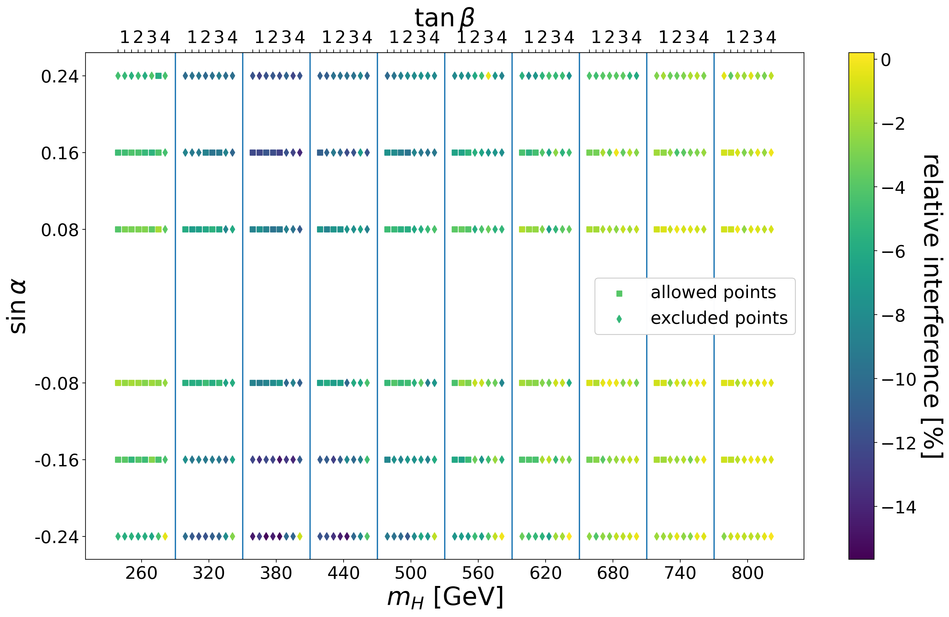
(d) The relative interference $\left(\Delta\sigma\right)_{\text{rel}}^{>}$ for $m_{hh}>m_{H}$.

(e) The total interference sum $\left(\Delta\sigma\right)_{\text{abs}}^{\sum}=\left|\left(\Delta\sigma\right)_{\text{abs}}^{<}\right|+\left|\left(\Delta\sigma\right)_{\text{abs}}^{>}\right|$.

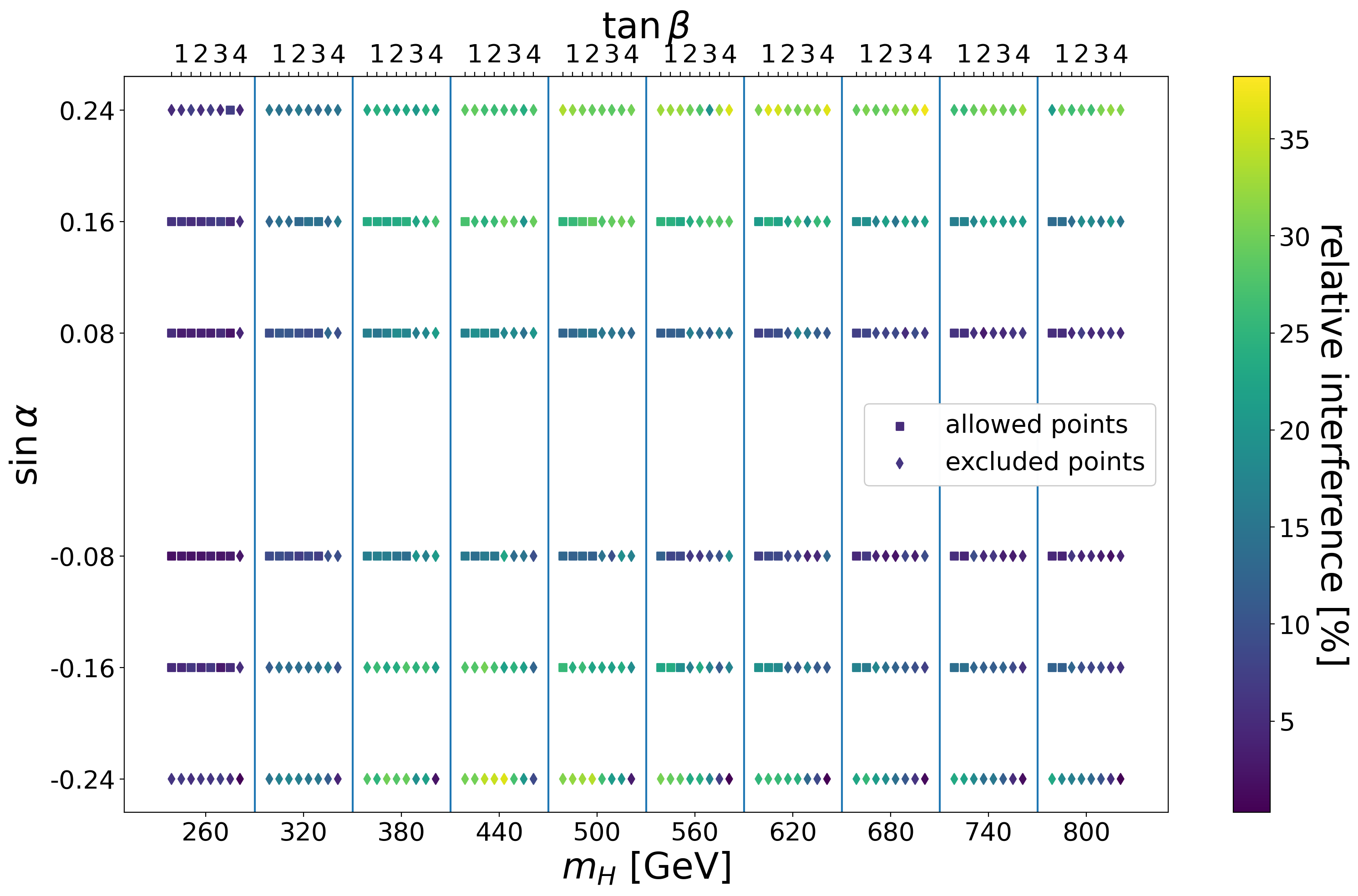
(f) The relative interference sum $\left(\Delta\sigma\right)_{\text{rel}}^{\sum}=\left|\left(\Delta\sigma\right)_{\text{rel}}^{<}\right|+\left|\left(\Delta\sigma\right)_{\text{rel}}^{>}\right|$.

Figure 6: Interferences for invariant di-Higgs masses $m_{hh}$ above and below the heavy scalar mass $m_{H}$. Bins on the x-axis represent different $m_{H}$ values, ordered by increasing $\tan\beta$ within each bin. The y-axis shows $\sin\alpha$, excluding $\sin\alpha=0$ (SM case). Circles represent allowed points and triangles represent the points that do not pass the scan constraints described in Section II. The colours of the points indicate the size of $\left(\Delta\sigma\right)_{\text{abs}}^{<}$, $\left(\Delta\sigma\right)_{\text{rel}}^{<}$, $\left(\Delta\sigma\right)_{\text{abs}}^{>}$, $\left(\Delta\sigma\right)_{\text{rel}}^{>}$, $\left(\Delta\sigma\right)_{\text{abs}}^{\sum}$, and $\left(\Delta\sigma\right)_{\text{rel}}^{\sum}$ for the upper-left, upper-right, middle-left, middle-right, lower-left, and lower-right, plots, respectively.

In order to relate the dependence of the cross-sections to the dependence of the involved couplings, we also display the triple Higgs couplings $\lambda_{hhh}$ and $\lambda_{Hhh}$ defined in Eq. (II.1), as well as the total widths of the two Higgs bosons, $\Gamma_{h}$ and $\Gamma_{H}$ in Figure 7. From Figure 7a, we observe that $\kappa_{\lambda_{hhh}}$ has a larger deviation from the SM for larger $|\alpha|$ values, but never exceeds 1. Figure 7b shows that $\lambda_{Hhh}$ has the sign of the mixing angle for the points considered here. These patterns reflect the analytic behaviour of the couplings for small values of $\sin\alpha$, see Eq. (II.1). Figure 7c demonstrates that $\Gamma_{h}$ only depends the mixing angle and Figure 7d shows that $\Gamma_{H}$ increases with both the absolute value of the mixing angle and $\tan\beta$, and reaches maximal ratios of $\Gamma_{H}/m_{H}\,\sim\,0.012$ for the points still allowed by current constraints.

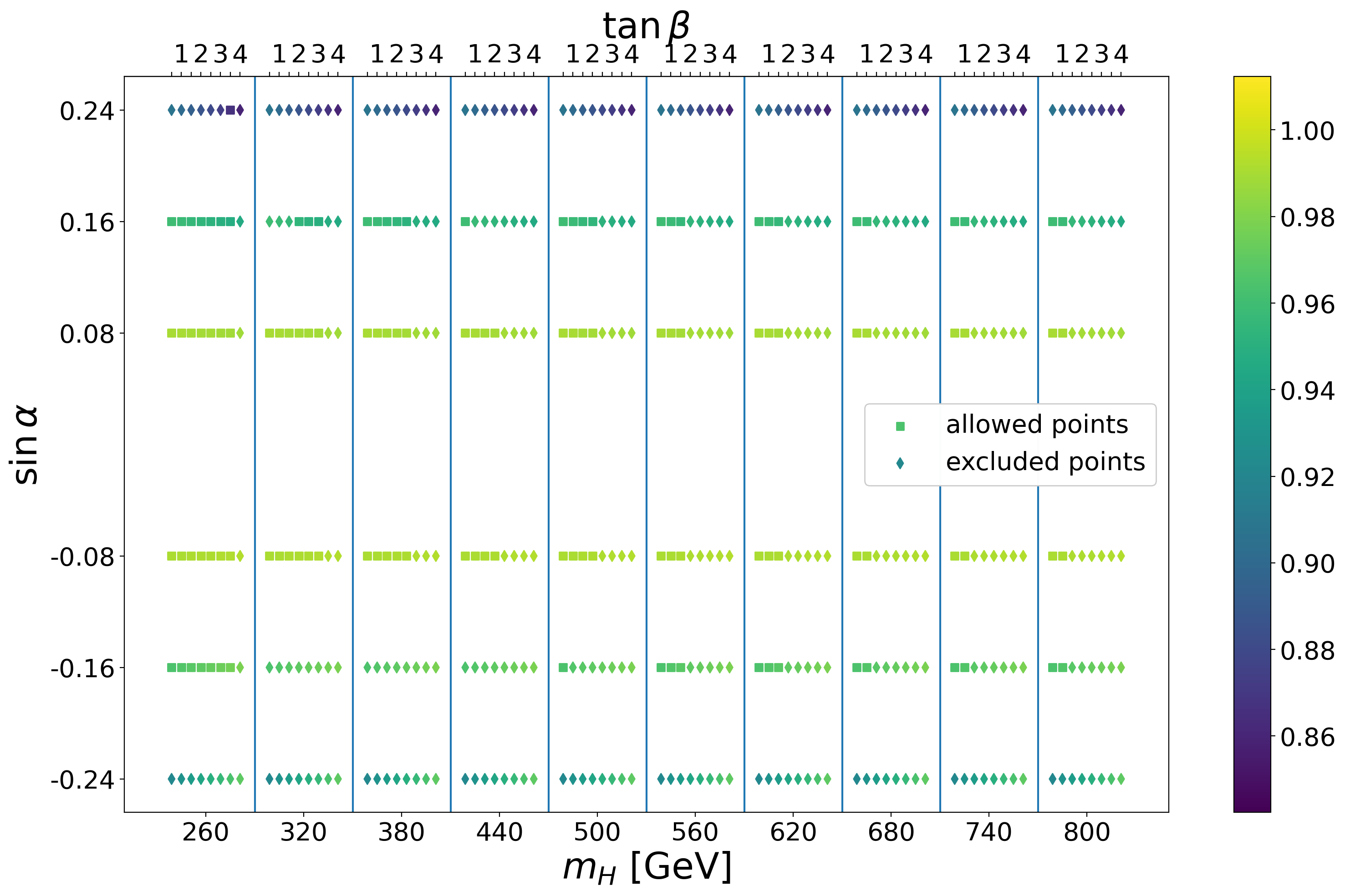
(a) $\kappa_{\lambda_{hhh}}$

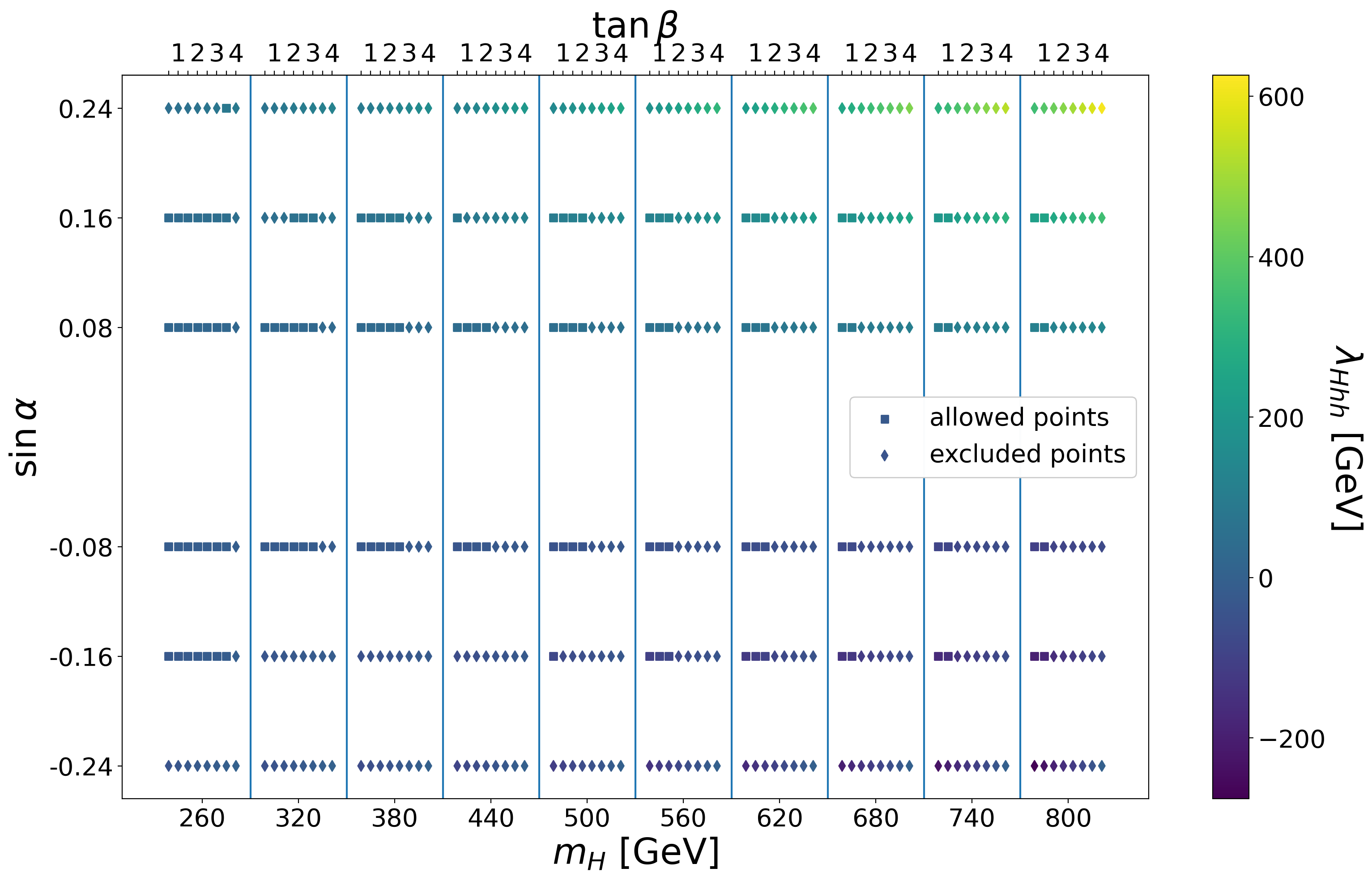
(b) $\lambda_{Hhh}$

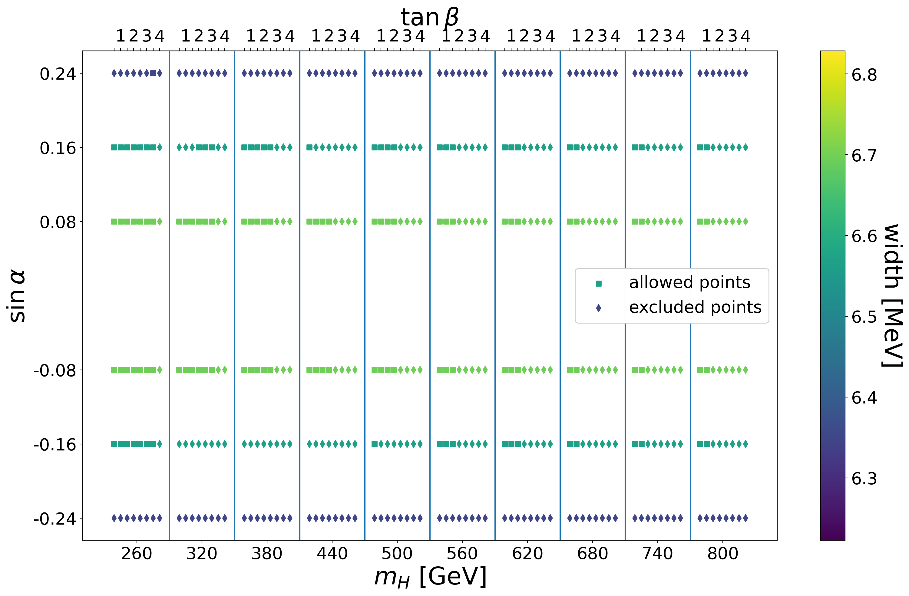
(c) $\Gamma_{h}$

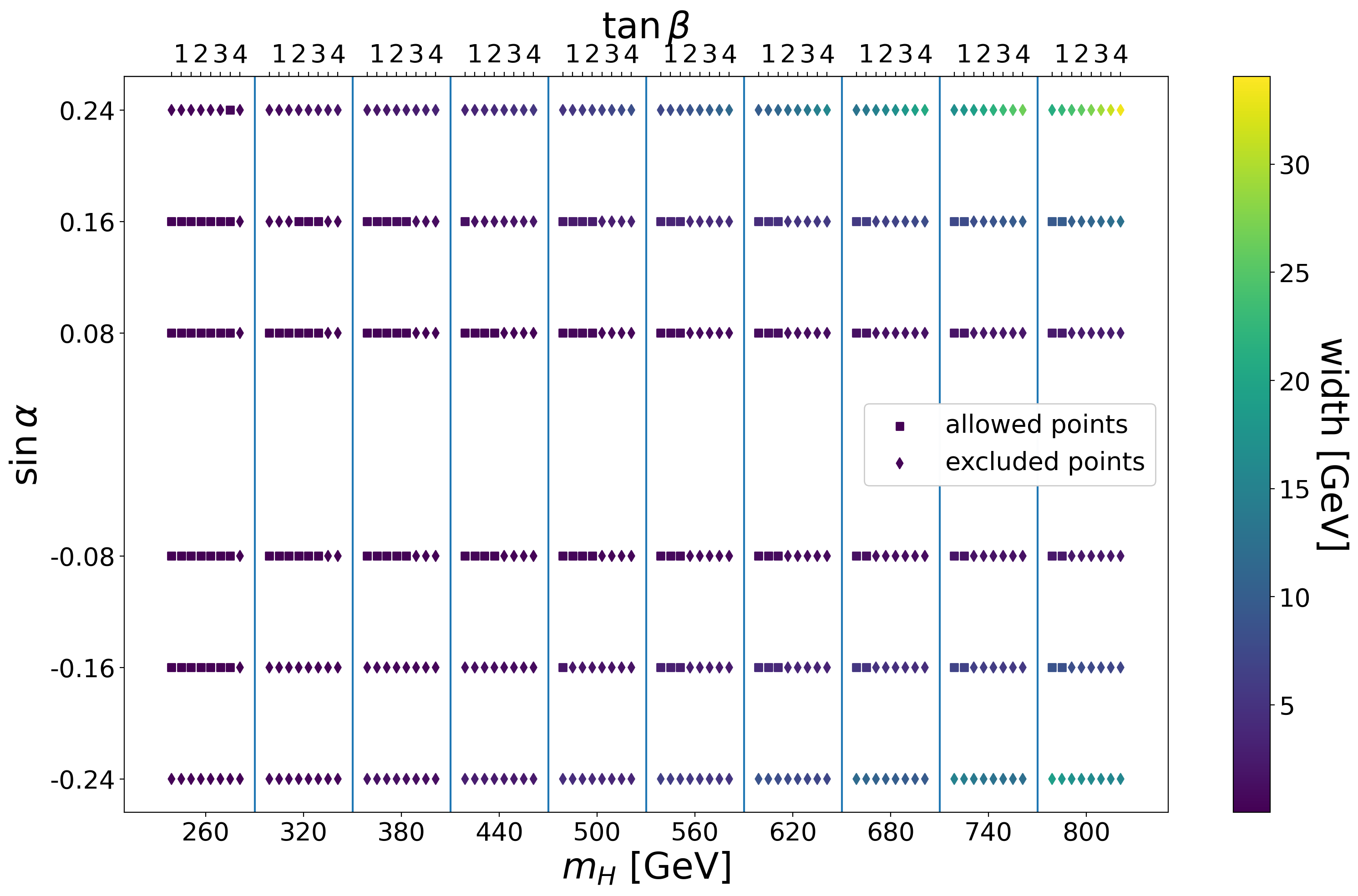
(d) $\Gamma_{H}$

Figure 7: The different bins on the x-axis show the different values of $m_{H}$ investigated and inside the bins the points are ordered by the corresponding $\tan\beta$ values from left to right. The $\sin\alpha$ value is shown on the y-axis, where $\sin\alpha=0$ is left out, as it corresponds to the SM-case. Circles represent allowed points and triangles represent the points that do not pass the scan constraints described in Section II. The colours of the points indicate the size of $\kappa_{\lambda_{hhh}}$, $\lambda_{Hhh}$, $\Gamma_{h}$, and $\Gamma_{H}$ for the upper-left, upper-right, lower-left, and lower-right plots, respectively.

A small comment is in order: the reader may notice that the width of the SM-like scalar is around $\sim\,6\,{\rm MeV}$, which is in principle compatible with the current experimental values of $3.2^{+2.4}_{-1.7}\,{\rm MeV}$ CMS:2022ley and $4.5^{+3.3}_{-2.5}\,{\rm MeV}$ ATLAS:2023dnm from off-shell $H\rightarrow ZZ$ measurements by CMS and ATLAS, respectively, but is not in agreement with the most up to date theoretical prediction of $\Gamma_{125}\,\sim\,4\,{\rm MeV}$ as e.g. documented in Ref. LHCHiggsCrossSectionWorkingGroup:2016ypw . This is mainly due to the fact that in naive MadGraph calculations, the bottom mass in the $h\,\rightarrow\,b\,\bar{b}$ decay width is defined as the on-shell and not the $\overline{\text{MS}}$ mass, which takes a much smaller value at the scale $\mu\,\equiv\,125\,{\,\rm GeV}$. This in principle also manifests itself in discrepancies of the branching ratios of the $125\,{\,\rm GeV}$ scalar. However, as in our scenario the $125\,{\,\rm GeV}$ particle only appears in highly off-shell scenarios, we did not modify the total width but keep the LO calculated value from MadGraph in our simulations.

VI Modelling interference effects using reweighting

There are numerous examples of extended Higgs sector models that include an additional scalar that can impact the di-Higgs cross-section and differential distributions, see e.g. Ref. wg3ext for an overview of models currently investigated by the LHC experiments. The final di-Higgs spectrum depends on the parameters of the model. For example, in our investigated singlet model there are three free parameters that affect the relative contributions of the diagrams shown in Figure 2 to the total cross-section, and there are countless other models that may contain even more free parameters. While in principle it is possible to generate Monte Carlo (MC) events for different combinations of parameters, and simulate the detector responses, the computational resources required would be immense. We have therefore developed a tool, HHReweighter, utilising a matrix-element (ME) reweighting method to reduce the total CPU time required to model the full parameter space. The MEs are computed using MadGraph5_amc@nlo (version 2.6.7). Our tool is publicly available in GitLab reweight_repo .

VI.1 Reweighting LO samples

LO-accurate ME reweighting methods work by reweighting events of a reference sample by a weight, $w$, given by

$$w=\frac{|\mathcal{M}_{\mathrm{target}}|^{2}}{|\mathcal{M}_{\mathrm{ref}}|^{2}},$$ (26)

where $\mathcal{M}_{\mathrm{ref}}$ is the ME used in the generation of the reference sample and $\mathcal{M}_{\mathrm{target}}$ is the ME for the target model/model-parameters. While it is possible to compute $|\mathcal{M}_{\mathrm{target}}|^{2}$ for all interesting models/parameters, and this is certainly less CPU intensive than performing full event simulations, it would still require substantial computing resources to obtain all the final distributions in fits to data.

To mitigate this limitation, our strategy is to first decompose the squared ME describing di-Higgs production into several terms corresponding to the three diagrams shown in Figure 2, as well as the corresponding interference terms. This includes three squared terms corresponding to the $\Box$, $\mathrm{S_{h}}$, and $\mathrm{S_{H}}$ diagrams, plus three cross-terms describing the interferences between these contributions: $\mathrm{S_{h}}{\text{-}}\Box$, $\mathrm{S_{H}}{\text{-}}\Box$, and $\mathrm{S_{H}}{\text{-}}\mathrm{S_{h}}$. The MEs depend on the Yukawa couplings of the $h$ and $H$ to the top quark, denoted $y_{t}^{h}$ and $y_{t}^{H}$, respectively, the Yukawa couplings to the bottom quark, denoted $y_{b}^{h}$ and $y_{b}^{H}$, respectively, and the $\lambda_{hhh}$ and $\lambda_{Hhh}$ trilinear couplings. For convenience, we compute each of the MEs setting $y_{t}^{h}=y_{t}^{H}=y_{t}^{\mathrm{SM}}$, $y_{b}^{h}=y_{b}^{H}=y_{b}^{\mathrm{SM}}$, and $\lambda_{hhh}=\lambda_{Hhh}=\lambda_{\mathrm{SM}}$, where $y_{t}^{\mathrm{SM}}$ ($y_{b}^{\mathrm{SM}}$) and $\lambda_{\mathrm{SM}}$ are the top (bottom) Yukawa and trilinear couplings of the SM Higgs sector. We denote the squared MEs $\mathcal{M}_{i}^{2}$ (where $i=\Box,\mathrm{S_{h}},\mathrm{S_{H}},\mathrm{S_{h}}{\text{-}}\Box,\mathrm{S_{H}}{\text{-}}\Box,\mathrm{S_{H}}{\text{-}}\mathrm{S_{h}}$) in the following. For the interference terms, we use the shorthand notation

$$\widetilde{\mathcal{M}}^{2}_{a\text{-}b}\equiv 2\text{Re}\left[\mathcal{M}_{a}\,\mathcal{M}^{*}_{b}\right].$$ (27)

The total squared ME for any model can then be constructed by a linear combination of these terms according to

$$\begin{split}|\mathcal{M}_{\mathrm{total}}|^{2}=&\mathcal{M}_{\Box}^{2}\cdot(\kappa_{q}^{h}{})^{4}+\mathcal{M}_{\mathrm{S_{h}}}^{2}\cdot(\kappa_{q}^{h}{})^{2}\kappa_{\lambda_{hhh}}^{2}+\widetilde{\mathcal{M}}_{\mathrm{S_{h}}{\text{-}}\Box}^{2}\cdot(\kappa_{q}^{h}{})^{3}\kappa_{\lambda_{hhh}}+\mathcal{M}_{\mathrm{S_{H}}}^{2}(m_{H},\Gamma_{H})\cdot(\kappa_{q}^{H}{})^{2}\kappa_{\lambda_{Hhh}}^{2}\\ &+\widetilde{\mathcal{M}}_{\mathrm{S_{H}}{\text{-}}\Box}^{2}(m_{H},\Gamma_{H})\cdot(\kappa_{q}^{h}{})^{2}\kappa_{q}^{H}{}\kappa_{\lambda_{Hhh}}+\widetilde{\mathcal{M}}_{\mathrm{S_{H}}{\text{-}}\mathrm{S_{h}}}^{2}(m_{H},\Gamma_{H})\cdot\kappa_{q}^{h}{}\kappa_{q}^{H}{}\kappa_{\lambda_{hhh}}\kappa_{\lambda_{Hhh}},\end{split}$$ (28)

where $\kappa_{q}^{H}\equiv\frac{y_{t}^{H}}{y_{t}^{\mathrm{SM}}}=\frac{y_{b}^{H}}{y_{b}^{\mathrm{SM}}}$, $\kappa_{q}^{h}\equiv\frac{y_{t}^{h}}{y_{t}^{\mathrm{SM}}}=\frac{y_{b}^{h}}{y_{b}^{\mathrm{SM}}}$, and $\kappa_{\lambda_{Hhh}}\equiv\frac{\lambda_{Hhh}}{\lambda_{\mathrm{SM}}}$. We note that $\mathrm{S_{H}}$, $\mathrm{S_{H}}{\text{-}}\Box$, and $\mathrm{S_{H}}{\text{-}}\mathrm{S_{h}}$ terms also depend on the assumed values of $m_{H}$ and $\Gamma_{H}$.

The $\mathcal{M}_{i}^{2}$ values can be used to compute weights for the individual components allowing the di-Higgs distributions to be decomposed into the individual terms. An example of this is shown in Figure 8, for $m_{H}=600\,{\,\rm GeV}$ and $\Gamma_{H}=12\,{\,\rm GeV}$. All distributions are displayed for $\kappa_{q}^{h}=\kappa_{q}^{H}=\kappa_{\lambda_{hhh}}=\kappa_{\lambda_{Hhh}}=1$.

We briefly summarise the procedure we used to obtain this figure:

• We generate an event sample $S_{\text{SM}}$ for the pure SM process $pp\,\rightarrow\,h\,h$, that includes $\Box$, $\mathrm{S_{h}}$, and $\mathrm{S_{h}}{\text{-}}\Box$ contributions. From this sample, all but the $\mathrm{S_{H}}$ distributions are obtained via Eq. (26), with $|\mathcal{M}_{\text{target}}|^{2}$ given by the respective term of Eq. (28), and where $|\mathcal{M}_{\text{ref}}|^{2}$ corresponds to the squared matrix element for the SM process.

• A second sample $S_{2}$ is generated that corresponds to the resonant $s$-channel contribution. This is used for the distribution denoted by $\mathrm{S_{H}}$ .

We will comment on the validation of this procedure below.

In Figure 9, we also illustrate the effect of $\Gamma_{H}$ on one of the interference terms, where again contributions have been obtained as described above. All distributions are shown for $\kappa_{q}^{h}=\kappa_{q}^{H}=\kappa_{\lambda_{Hhh}}=1$.

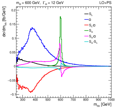
Figure 8: The di-Higgs mass distributions split into the individual contributions corresponding to the three diagrams in Figure 2 and the interference terms. The non-resonant SM-like contributions from the $\Box$, $\mathrm{S_{h}}$, and $\mathrm{S_{h}}{\text{-}}\Box$ terms are shown in blue, black, and red, respectively. The $\mathrm{S_{H}}$ resonant contributions is displayed in green. The interference between the $\mathrm{S_{H}}$ and the $\Box$ ($\mathrm{S_{h}}$) diagrams is shown in magenta (cyan). All distributions are shown for $\kappa_{q}^{h}=\kappa_{q}^{H}=\kappa_{\lambda_{hhh}}=\kappa_{\lambda_{Hhh}}=1$.

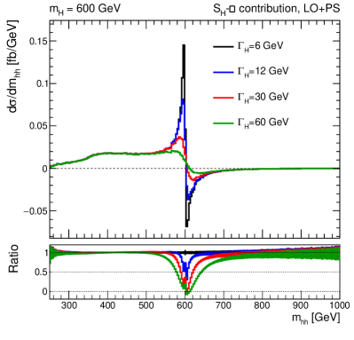
Figure 9: The di-Higgs mass distributions for the $\mathrm{S_{H}}{\text{-}}\Box$ interference term for different values of $\Gamma_{H}$. All distributions are shown for $\kappa_{q}^{h}=\kappa_{q}^{H}=\kappa_{\lambda_{Hhh}}=1$. The lower panel shows the ratio of the distributions with respect to $\Gamma_{H}=6\,{\,\rm GeV}$.

After the decomposition into the individual terms in Eq. (28), it is possible for the experimental searches to be conducted in such a way as to allow for reinterpretations in different models, as follows:

• Three distributions are produced for the $\Box$, $\mathrm{S_{h}}$, and $\mathrm{S_{h}}{\text{-}}\Box$ contributions, which do not depend on $m_{H}$ or $\Gamma_{H}$.

• Distributions for the $\mathrm{S_{H}}$, $\mathrm{S_{H}}{\text{-}}\Box$, and $\mathrm{S_{H}}{\text{-}}\mathrm{S_{h}}$ terms can be produced for several values of $m_{H}$ and $\Gamma_{H}$. The number of $\Gamma_{H}$ and $m_{H}$ values to be considered depends on the experimental resolution. For example, in Section IV we estimated the $m_{hh}$ resolution in the 4$b$ final state to be $\sim 6\%$; in this case we consider $\sim 4$ values of $\Gamma_{H}$ for each mass point as sufficient to take into account widths effects for $\frac{\Gamma_{H}}{m_{H}}<20\%$. The usual interpolation methods can be use to obtain distributions for intermediate points.

• The physics model in question predicts the values $\kappa_{q}^{h}$, $\kappa_{q}^{H}$, $\kappa_{\lambda_{hhh}}$, $\kappa_{\lambda_{Hhh}}$, and $\Gamma_{H}$ depending on the model parameters. For example, in the singlet model these are computed as a function of the $\tan\beta$, $\sin\alpha$, and $m_{H}$ parameters as

  $$\begin{split}\kappa_{q}^{h}&=\cos\alpha,\\ \kappa_{q}^{H}&=\sin\alpha,\\ \kappa_{\lambda_{hhh}}&=\cos^{3}{\alpha}-\tan\beta\sin^{3}{\alpha},\\ \kappa_{\lambda_{Hhh}}&=\frac{2m_{h}^{2}+m_{H}^{2}}{m_{h}^{2}}\,\frac{\sin\left(2\alpha\right)}{2}(\cos{\alpha}+\tan\beta\sin{\alpha}),\end{split}$$ (29)

  and the width is given in Eq. (II.1). Using these predictions, the total signal distribution is then constructed by combining the individual distributions according to Eq. (28).

Our tool gives the user the option to reweight either the SM non-resonant di-Higgs process or a resonant $\mathrm{S_{H}}$ sample. In principle, both options should give the same distributions within statistical uncertainties. However, in practise one needs to be careful to make sure the MC samples being reweighted are sufficiently populated in phase-space regions where $|\mathcal{M}_{\mathrm{target}}|^{2}$ is non-vanishing Mattelaer:2016gcx , to ensure statistical uncertainties do not become too large. With this in mind, we take the following approach to obtain distributions for each of the terms in Eq. (28). We obtain the $\Box$, $\mathrm{S_{h}}$, $\mathrm{S_{h}}{\text{-}}\Box$, $\mathrm{S_{H}}{\text{-}}\Box$, and $\mathrm{S_{H}}{\text{-}}\mathrm{S_{h}}$ terms by reweighting the SM non-resonant MC samples. To obtain the $\mathrm{S_{H}}$ distribution for a $m_{H}^{\mathrm{target}}$-$\Gamma_{H}^{\mathrm{target}}$ point, we reweight an $\mathrm{S_{H}}$ MC sample generated with the same $m_{H}$, and we ensure that the $\Gamma_{H}$ is not too far from $\Gamma_{H}^{\mathrm{target}}$.

Figure 10 shows examples of the reweighted distributions (blue) compared to the distributions obtained from a MC sample generated directly for the target model parameters (black). The distributions are shown for $m_{hh}$ and $p_{\mathrm{T}}$ of the leading $h$. However, several other kinematic and angular variables were analysed and found to have the same level of agreement.

In this case the target parameter points are $\sin\alpha=0.17$, $\tan\beta=1.5$, and $m_{H}=600\,{\,\rm GeV}$, which yields a predicted width of $5\,{\,\rm GeV}$. We obtain the $\mathrm{S_{H}}$ component by reweighting an $\mathrm{S_{H}}$ MC sample with $\Gamma_{H}=12\,{\,\rm GeV}$ and $\kappa_{\lambda_{Hhh}}=\kappa_{q}^{H}=1$, while a sample of SM di-Higgs events is used to obtain the other terms, as described above. The red line in Figure 10 shows the $m_{hh}$ spectrum for the MC events used in the reweighting procedure before the reweighting is applied for comparison. The distributions obtained for the reweighted events match the directly generated MC sample within the statistical uncertainties. The method is additionally validated for several other benchmark points as shown in Appendix B.

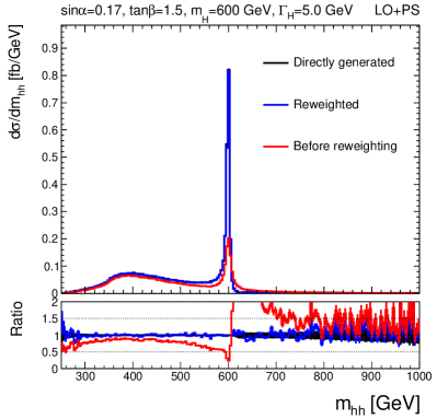
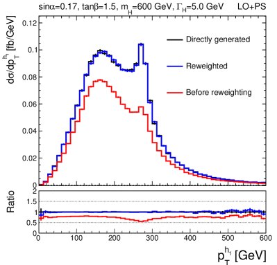
Figure 10: The reweighting method is validated by comparing the reweighted di-Higgs mass (left) and leading $h$ $p_{\mathrm{T}}$ (right) distributions (blue) to the distributions obtained by directly simulating the di-Higgs events for a set of parameter points (black). The red distribution corresponds to the MC events used for the reweighting, before the weights have been applied. On the left, the blue line overlays exactly the black points including error bars.

VI.2 Including higher-order corrections

The discussions so far have focused on MC events generated at LO. However, it is well known that the LO cross-section for gluon-fusion is significantly different compared to higher-order predictions (see e.g. Ref. LHCHiggsCrossSectionWorkingGroup:2016ypw and references therein). It is therefore necessary to correct the LO cross-section through the application of K-factors to account for this. The NNLO cross-sections for the $\Box$, $\mathrm{S_{h}}$, and $\mathrm{S_{h}}{\text{-}}\Box$ components deFlorian:2017qfk ; Buchalla:2018yce ; Grazzini:2018bsd ; Amoroso:2020lgh are used to define K-factors for these terms, which we call $K_{\Box}$, $K_{\mathrm{S_{h}}}$, and $K_{\mathrm{S_{h}}{\text{-}}\Box}$, respectively. For the $\mathrm{S_{H}}$, $\mathrm{S_{H}}{\text{-}}\Box$, and $\mathrm{S_{H}}{\text{-}}\mathrm{S_{h}}$ components, no dedicated NNLO predictions are provided. However, NNLO predictions are available for the production of a single undecayed SM-like $H$ ($gg\rightarrow H$) LHCHiggsCrossSectionWorkingGroup:2016ypw , and we use these predictions to define the K-factor for the $\mathrm{S_{H}}$ term:

$$K_{\mathrm{S_{H}}}=\frac{\sigma_{\mathrm{NNLO}}(gg\rightarrow H)}{\sigma_{\mathrm{LO}}(gg\rightarrow H)},$$ (30)

where $\sigma_{\mathrm{LO}}$ is also computed for single-Higgs production for consistency using MadGraph5_amc@nlo. To define K-factors for the $\mathrm{S_{H}}{\text{-}}\Box$ and $\mathrm{S_{H}}{\text{-}}\mathrm{S_{h}}$ terms we propose the ansatz:

$$\begin{split}K_{\mathrm{S_{H}}{\text{-}}\Box}&=\sqrt{K_{\mathrm{S_{H}}}K_{\Box}}~{}\mathrm{and}\\ K_{\mathrm{S_{H}}{\text{-}}\mathrm{S_{h}}}&=\sqrt{K_{\mathrm{S_{H}}}K_{\mathrm{S_{h}}}}.\end{split}$$ (31)

Table 3 lists the LO and NNLO cross-sections and the computed K-factors. All cross-sections are computed for $\kappa_{q}^{h}=\kappa_{q}^{H}=\kappa_{\lambda_{hhh}}=\kappa_{\lambda_{Hhh}}=1$. The cross-sections displayed for the $\mathrm{S_{H}}$, $\mathrm{S_{H}}{\text{-}}\Box$, and $\mathrm{S_{H}}{\text{-}}\mathrm{S_{h}}$ terms are computed for $m_{H}=600\,{\,\rm GeV}$ and $\Gamma_{H}=5\,{\,\rm GeV}$.

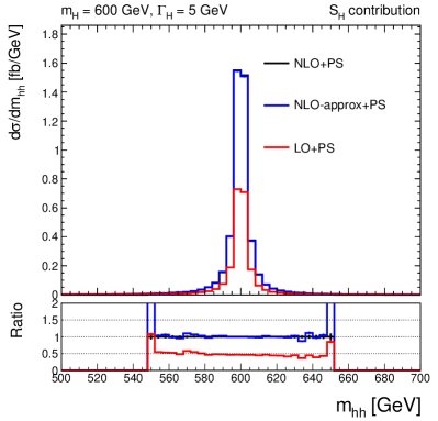
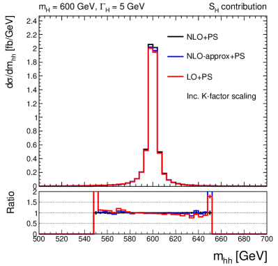
Figure 14: The di-Higgs mass distributions obtained for the $\mathrm{S_{H}}$ component. The NLO prediction (black) is compared to the approximate NLO distribution obtained by reweighting the NLO $\mathrm{S_{H}}$ MC sample (blue) and the LO distribution (red). The plot on the left (right) shows the distributions before (after) the NNLO K-factor scaling is applied.

We produce di-Higgs mass distributions for each of the terms in Eq. (28) generated at LO before and after the application of the K-factors. These distributions are shown by the red lines in Figures 11–16. The left and right plots show the distributions before and after the K-factor applications, respectively. We also compare the LO distributions to NLO predictions for cases where MC production is possible in POWHEG, namely the $\Box$, $\mathrm{S_{h}}$, $\mathrm{S_{h}}{\text{-}}\Box$, and $\mathrm{S_{H}}$ terms. These predictions are shown by the black lines in the figures.

While the pure resonant contributions as well as all non-resonant contributions are readily available at NLO, there is currently no MC on the market that simulates the full contribution including all interference terms at that order. This motivates us to define an approach that tries to remedy this by mimicking the expected contributions, to be confirmed once the according tools become available in the future. Furthermore, some transverse variables, such as $p_{T}^{hh}$, typically vary widely between LO and NLO and in principle require the description via NLO kinematics, including real radiation. We therefore define an approximate scheme for NLO results (labelled “NLO-approx”), which we obtain by reweighting NLO MC events using LO ME weights.

In the POWHEG description Frixione:2007nu , the largest part of the events is simulated with NLO kinematics, giving rise to an additional hard real emission parton. In order to map this to the LO matrix elements used for reweighting, we apply the following procedure: We “ignore” the additional parton when we perform the reweighting. Technically, this is obtained in the following way. We take the two outgoing $h$ four-momenta from the ME and boost to the di-Higgs rest frame. We then obtain the four-momenta for the incoming gluons by requiring both gluons to have zero transverse momentum, and equal and opposite longitudinal momentum, also requiring four-momentum conservation between incoming and outgoing particles. When estimating the MEs we also average over all possible spin-states of the incoming gluons. An NLO SM di-Higgs sample is reweighted to obtain the NLO-approx $\Box$, $\mathrm{S_{h}}$, and $\mathrm{S_{h}}{\text{-}}\Box$, $\mathrm{S_{H}}{\text{-}}\Box$, and $\mathrm{S_{H}}{\text{-}}\mathrm{S_{h}}$ terms, while an NLO $\mathrm{S_{H}}$ sample with $\Gamma_{H}=12\,{\,\rm GeV}$ is reweighted to obtain the NLO-approx $\mathrm{S_{H}}$ sample for a different width ($\Gamma_{H}=5\,{\,\rm GeV}$ in this case). The NLO-approx results are shown by the blue lines in the figures. The total rate in the NLO-approx method is obtained using the newly determined weights, derived from the LO matrix elements, for each separate contribution and phase space point. Furthermore, in order to include corrections to the overall rate to NNLO, we define an equivalent set of K-factors accounting for the scaling of the NLO and NLO-approx cross-sections to the NNLO predictions. The NLO(-approx) cross-sections and K-factors are also displayed in Table 3.

We remind the reader that our method for simulating $\mathrm{S_{H}}$ at NLO generates undecayed $gg\rightarrow H$ events using POWHEG and then performs the $H\rightarrow hh$ decays using PYTHIA (as described in Section IV). For this reason, the cross-section determined from POWHEG does not include the $H\rightarrow hh$ branching ratio. To obtain the correct $\mathrm{S_{H}}$ cross-section we thus multiply the undecayed $gg\rightarrow H$ cross-section by the branching ratio which is determined using the above settings for the couplings, that leads to $\Gamma(H\,\rightarrow\,h\,h)\,=\,0.061\,{\,\rm GeV}$ using MadGraph5_amc@nlo at LO, and then dividing by the respective width of 5  GeV, leading to a BR of 0.012.

Term	$\sigma_{\mathrm{LO}}$	$\sigma_{\mathrm{NLO}}$	$\sigma_{\sim\mathrm{NLO}}$	$\sigma_{\mathrm{NNLO}}$	$K_{i}^{\mathrm{LO}}$	$K_{i}^{\mathrm{NLO}}$	$K_{i}^{\sim\mathrm{NLO}}$
$\Box$	27.50 fb	60.37 fb	58.45 fb	70.39 fb	2.56	1.17	1.20
$\mathrm{S_{h}}$	3.70 fb	9.17 fb	8.31 fb	11.06 fb	2.99	1.21	1.33
$\mathrm{S_{h}}{\text{-}}\Box$	-18.08 fb	-42.35 fb	-39.57 fb	-50.41 fb	2.79	1.19	1.27
$\mathrm{S_{H}}$ (undecayed)	0.73 pb	1.51 pb	–	2.00 pb	2.74	1.33	1.30
$\mathrm{S_{H}}$	8.91 fb	18.43 fb	18.78 fb	–	2.74	1.33	1.30
$\mathrm{S_{H}}{\text{-}}\Box$	5.10 fb	–	10.68 fb	–	2.65	–	1.25
$\mathrm{S_{H}}{\text{-}}\mathrm{S_{h}}$	-1.40 fb	–	-3.02 fb	–	2.87	–	1.32

Table 3: The K-factors used to correct the LO, NLO, and NLO-approx samples to the NNLO cross-sections. The cross-sections used in the calculations of the K-factors are also displayed. The NLO-approx values are indicated by the “$\sim\mathrm{NLO}$” sub/super-scripts. The K-factors are defined as $K^{j}\equiv\frac{\sigma_{\mathrm{NNLO}}}{\sigma_{j}}$, where $j$ denotes the perturbative order. The above table is computed for $m_{H}\,=\,600\,{\,\rm GeV}$, $\Gamma_{H}\,=\,5\,{\,\rm GeV}$, and $\kappa_{q}^{h}=\kappa_{q}^{H}=\kappa_{\lambda_{hhh}}=\kappa_{\lambda_{Hhh}}=1$. Please see text for details on the branching ratios used in the decayed $\mathrm{S_{H}}$ cross section calculation.

As expected, Figures 11–13 show a significant difference between the LO and NLO yields due to the differences in the cross-sections. However, after application of the K-factors the yields agree (by construction) and we observe a good agreement in the shapes of the distributions compared to the NLO, indicating that LO samples are adequate for describing the $m_{hh}$ spectrum. The shapes of the NLO-approx distributions also agree well with the NLO distributions, and in this case the yields/cross-section before application of the K-factors are also noticeable quite similar to the NLO results. Figures 15 and 16 show the LO and NLO-approx distributions for the $\mathrm{S_{H}}{\text{-}}\Box$ and $\mathrm{S_{H}}{\text{-}}\mathrm{S_{h}}$ terms, respectively. While no comparisons to the full NLO results are possible in this case, the agreement between the shapes and the yields (after K-factor scaling) of the LO and NLO-approx distributions gives further confidence in the description of the $m_{hh}$ spectrum by the LO MC samples after reweighting.

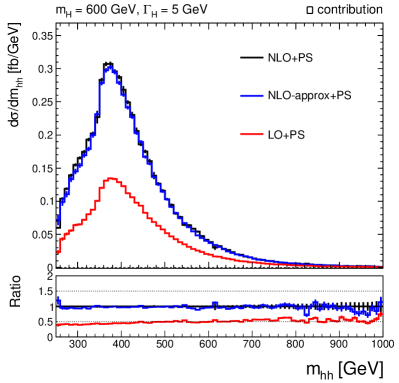
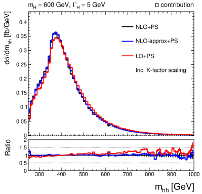
Figure 11: The di-Higgs mass distributions obtained for the $\Box$ component. The NLO prediction (black) is compared to the approximate NLO distribution obtained by reweighting the NLO SM di-Higgs MC (blue) and the LO distribution (red). The plot on the left (right) shows the distributions before (after) the NNLO K-factor scaling is applied.

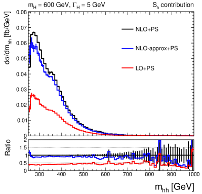
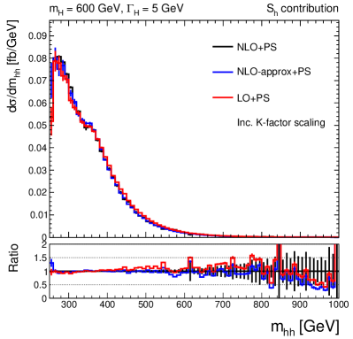
Figure 12: The di-Higgs mass distributions obtained for the $\mathrm{S_{h}}$ component. The NLO prediction (black) is compared to the approximate NLO distribution obtained by reweighting the NLO SM di-Higgs MC (blue) and the LO distribution (red). The plot on the left (right) shows the distributions before (after) the NNLO K-factor scaling is applied.

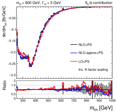
Figure 13: The di-Higgs mass distributions obtained for the $\mathrm{S_{h}}{\text{-}}\Box$ component. The NLO prediction (black) is compared to the approximate NLO distribution obtained by reweighting the NLO SM di-Higgs MC (blue) and the LO distribution (red). The plot on the left (right) shows the distributions before (after) the NNLO K-factor scaling is applied.

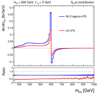
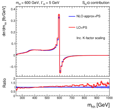
Figure 15: The di-Higgs mass distributions obtained for the $\mathrm{S_{H}}{\text{-}}\Box$ component. The NLO prediction (black) is compared to the approximate NLO distribution obtained by reweighting the NLO SM di-Higgs MC (blue) and the LO distribution (red). The plot on the left (right) shows the distributions before (after) the NNLO K-factor scaling is applied.

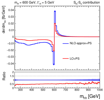
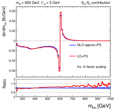
Figure 16: The di-Higgs mass distributions obtained for the $\mathrm{S_{H}}{\text{-}}\mathrm{S_{h}}$ component. The NLO prediction (black) is compared to the approximate NLO distribution obtained by reweighting the NLO SM di-Higgs MC (blue) and the LO distribution (red). The plot on the left (right) shows the distributions before (after) the NNLO K-factor scaling is applied.

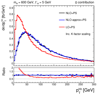
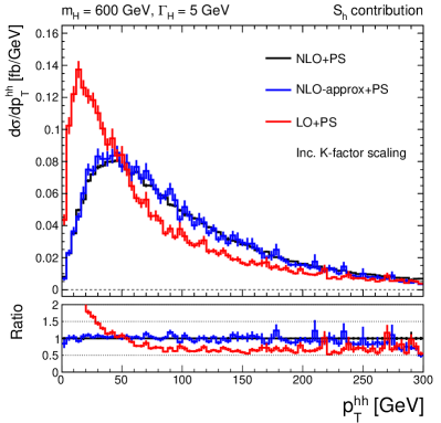
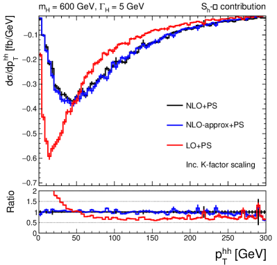
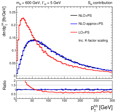
Figure 17: The di-Higgs $p_{\mathrm{T}}$ distributions obtained for the $\Box$ component (upper left), $\mathrm{S_{h}}$ component (upper right), $\mathrm{S_{h}}{\text{-}}\Box$ component (lower left), and $\mathrm{S_{H}}$ component (lower right). The NLO prediction (black) is compared to the approximate NLO distribution obtained by reweighting the NLO di-Higgs MC (blue) and the LO distribution (red). The NNLO K-factor scaling is applied in all cases.

While the LO MC gives a good description of the $m_{hh}$ spectrum, it is well know that the modelling of variables that are sensitive to the additional radiation are more problematic, as this is approximated by the parton shower. In Figure 17 we show an example of such a variable, the di-Higgs $p_{\mathrm{T}}$, $p_{\mathrm{T}}^{hh}$. The LO samples clearly tend to predict a softer $p_{\mathrm{T}}$ distribution compared to the NLO. In contrast, the agreement of the NLO-approx method is almost exact.

Finally, in support of the ansatz we made in Eq. (31), we make the following two observations:

1. As shown in Figures 15 and  16, the predicted $\mathrm{S_{H}}{\text{-}}\Box$ and $\mathrm{S_{H}}{\text{-}}\mathrm{S_{h}}$ yields (and equivalently the cross-sections) for the LO and NLO-approx methods after the K-factor scaling are in good agreement. The cross-sections predicted for the $\mathrm{S_{H}}{\text{-}}\Box$ term for LO and NLO-approx are 13.52 fb and 13.35 fb, respectively. While the cross-sections for the $\mathrm{S_{H}}{\text{-}}\mathrm{S_{h}}$ term are -4.02 fb and -4.00 fb. This demonstrates that the method is, at least, robust regardless of whether it is applied to LO or NLO samples.

2. We can apply the same ansatz to estimate the K-factors for the $\mathrm{S_{h}}{\text{-}}\Box$ term and compare to the K-factors computed directly from the NNLO cross-sections. The K-factors predicted via the ansatz are 2.77, 1.19, and 1.26 for the LO, NLO, and NLO-approx methods, respectively, which agree with the values presented in Table 3 within 1%.

VII Interference effects on differential distributions

We use the scans shown in Section V to define several interesting BM points. We select the BM points such that they exhibit interesting features that we will describe below. Additionally, we ensure that all points are accessible to experimental searches at the LHC, by requiring that the $gg\rightarrow H\rightarrow hh$ ($\mathrm{S_{H}}$-only) cross-section $\sigma_{\mathrm{S_{H}}}$, scaled by the K-factors as described in Section VI, is close to the experimental limits presented by the ATLAS Collaboration in Ref. ATLAS:2021tyg . To achieve this we require $\sigma_{\mathrm{S_{H}}}>\sigma_{\mathrm{ATLAS}}\times\sqrt{\frac{140}{L[\mathrm{fb}^{-1}]}}$, where $\sigma_{\mathrm{ATLAS}}$ is the expected limits from Ref. ATLAS:2021tyg , and $L$ is a target luminosity. We consider two values of $L$ equal to 400 $\mathrm{fb}^{-1}$ and 3000 $\mathrm{fb}^{-1}$, which approximately correspond to the expected luminosity recorded by each of the ATLAS/CMS detectors at the end of Run-3 (assuming Run-2+Run-3 are combined) and at the end of the LHC program, respectively.

Table 4 summarises the BM points, which will be described in more detail in the following sections. All points in the table satisfy the $\sigma_{\mathrm{S_{H}}}$ requirement for $L=3000~{}\mathrm{fb}^{-1}$, and we additionally indicate in the second to last column if the requirement is also satisfied for $L=400~{}\mathrm{fb}^{-1}$. In the following sections, we will state the parameters of the singlet model for the chosen benchmark scenarios and show distributions produced from MC events generated at LO in QCD. The K-factor scaling described in Section VI is also applied. We remind the reader than the shapes of the $m_{hh}$ distributions generated at LO were shown to agree very well with the NLO distributions, and thus we deem the LO samples to be sufficient for these comparisons. We note that the $p_{\mathrm{T}}^{hh}$ spectrum at LO does not accurately match the NLO predictions, therefore, any analysis relying on these or similar kinematic observables should be generated at NLO, as argued above.

Benchmark	$\sin\alpha$	$\tan\beta$	$m_{H}$	$\Gamma_{H}$	$\kappa_{\lambda_{hhh}}$	$\sigma$	$\sigma_{\mathrm{S_{H}}}$	Accessible	Feature
			[ GeV]	[ GeV]		[fb]	[fb]	in Run-3
BM1	0.16	1.0	620	4.6	0.96	50.5	13.5	✓	Max $\left(\Delta\sigma\right)_{\text{rel}}$
BM2	0.16	0.5	440	1.5	0.96	91.6	56.4	✓	Max $\left(\Delta\sigma\right)_{\text{rel}}^{\sum}$
BM3	0.16	0.5	380	0.8	0.96	119.8	90.1	✓	Max $\left(\Delta\sigma\right)_{\text{rel}}^{\sum}$ with $\left(\Delta\sigma\right)_{\text{rel}}<1\%$
BM4	-0.16	0.5	560	3.0	0.96	51.4	15.5	✓	Max non-res. within $m_{H}\pm 10\%$
BM5	0.08	0.5	500	0.6	0.99	40.6	8.1		Max non-res. within $m_{H}\pm 10\%$
BM6	0.16	1.0	680	6.1	0.96	44.8	8.4	✓	Max $m_{H}$
BM7	0.15	1.1	870	9.5	0.96	36.8	2.3		Max $m_{H}$
BM8	0.24	3.5	260	0.6	0.87	374.2	357.3	✓	Max $|\kappa_{\lambda_{hhh}}-1|$
BM9	0.16	1.0	800	9.8	0.96	38.9	3.6		Max $\frac{\Gamma_{H}}{m_{H}}$

Table 4: Overview of the investigated benchmark points. The values of the $\sin\alpha$, $\tan\beta$, and $m_{H}$ model parameters are shown. The values of $\Gamma_{H}$, $\kappa_{\lambda_{hhh}}$, $\sigma$, and $\sigma_{\mathrm{S_{H}}}$, which are fixed by the model parameters, are also displayed. The cross-sections are computed at LO and scaled by NNLO K-factors as described in Section VI. The second to last column indicates whether the points are expected to be accessible at the LHC by the end of Run-3. The last column gives a summary of the feature exhibited by the benchmark point.

VII.1 BM1

Our first BM point, BM1, is chosen as one of the points where the influence of the interference on the di-Higgs cross-section is maximal. Accordingly, we take a point with a relatively large value of $\left(\Delta\sigma\right)_{\text{rel}}$ (equal to 13%) from the points that are still allowed according to our scan specifications, which is found for $m_{H}=620\,{\,\rm GeV}$, $\sin\alpha=0.16$, and $\tan\beta=1.0$.

The $m_{hh}$ distributions for this BM with and without detector smearing are displayed in Figure 18. Smearing in this and all subsequent figures is performed according to the prescription discussed in Section IV. The figure compares the distributions for four different treatments of the di-Higgs modelling. The full di-Higgs distribution including both resonant and non-resonant diagrams and interference terms is shown in blue, the distribution neglecting the $\mathrm{S_{H}}{\text{-}}\Box$ and $\mathrm{S_{H}}{\text{-}}\mathrm{S_{h}}$ interference terms in shown in red (referred to as “no-interference” in the following), the $\mathrm{S_{H}}$-only distribution is shown in green, and the distribution obtained by fixing the non-resonant di-Higgs spectrum to the SM expectation and summing with the $\mathrm{S_{H}}$ distribution is shown in magenta (referred to as “SM+$\mathrm{S_{H}}$”).

The interference tends increase (decrease) the broader non-resonant-like continuum above (below) the resonant peak at $m_{H}\sim 620\,{\,\rm GeV}$. After detector smearing, the overall distribution exhibits an interesting double-peak structure. The interference also causes a shift in the position of the mass peak to slightly lower values, however, after smearing the shift in the peak position is not very noticeable. It is clear from comparing to the $\mathrm{S_{H}}$-only spectrum that neglecting the non-resonant terms altogether results in a failure to describe the double-peak structure, and it also results in an underestimation of the number of events close to the peak of around 35%. Including the non-resonant terms while neglecting only the $\mathrm{S_{H}}{\text{-}}\Box$ and $\mathrm{S_{H}}{\text{-}}\mathrm{S_{h}}$ interference terms clearly brings an improvement in the overall description of the spectrum. However, it still results in an underestimate of the height of the $\mathrm{S_{H}}$ peak by about 15%, and an under(over)-estimate of the non-resonant continuum of $\approx$ 15–30% (15–40%) below (above) the resonant peak. This clearly motivates the proper consideration of the interference effects when performing resonant searches. We also do not observe a significant difference between no-interference and SM+$\mathrm{S_{H}}$ distributions. This is because only small values of $\sin\alpha$ are still allowed by the experimental constraints and this results in $\kappa_{\lambda_{hhh}}$ and $\kappa_{q}^{h}$ values that are typically close to unity at LO. As will be shown in the subsequent sections, this feature is common to all BM points.

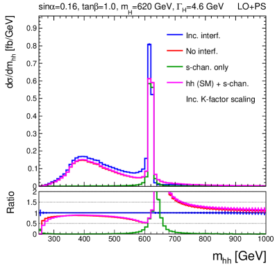
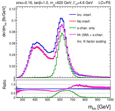
Figure 18: The di-Higgs mass distributions for BM1 before (left) and after (right) experimental smearing. The blue lines show the full di-Higgs spectrum including all interference terms. This is compared to the spectrum excluding the $\mathrm{S_{H}}{\text{-}}\Box$ and $\mathrm{S_{H}}{\text{-}}\mathrm{S_{h}}$ interference terms shown in red, the $H$ $s$-channel spectrum ($\mathrm{S_{H}}$) shown in green, and the incoherent sum of $\mathrm{S_{H}}$ and the SM di-Higgs spectrum in magenta.

We also show the distributions for several other variables in Figures 19-28. The variables displayed are: $p_{\mathrm{T}}^{hh}$, the $p_{\mathrm{T}}$ of the leading and sub-leading $h$, $p_{\mathrm{T}}^{h_{1}}$ and $p_{\mathrm{T}}^{h_{2}}$, the $p_{\mathrm{T}}$ of the leading and softest $b$-jets, $p_{\mathrm{T}}^{b_{1}}$ and $p_{\mathrm{T}}^{b_{4}}$, the $\mathrm{H}_{\mathrm{T}}$ of the four $b$-jets, the $\eta$ of the di-Higgs system, $\eta^{hh}$, the separation in $\eta$ of the two $h$, $\Delta\eta(h_{1},h_{2})$, the separation of the $\phi$ between the two $h$, $\Delta\phi(h_{1},h_{2})$, and the $\Delta R$ (where $\Delta R^{2}=\Delta\phi^{2}+\Delta\eta^{2}$) between the two $h$, $\Delta R(h_{1},h_{2})$. In general, the effect of the interference on the shapes of these variables is less significant than was observed for $m_{hh}$. The $p_{\mathrm{T}}^{hh}$ and $\eta^{hh}$ distributions in particular do not show any noticeable differences in shapes when neglecting the interference terms. There are more noticeable differences in the other distributions, however, the regions which have largest differences tend to occur in the tails and therefore probably do not have a very large impact on the experimental searches. The $\mathrm{S_{H}}$-only $p_{\mathrm{T}}^{h_{1}}$, $p_{\mathrm{T}}^{h_{2}}$, $p_{\mathrm{T}}^{b_{1}}$, $p_{\mathrm{T}}^{b_{4}}$, and $\mathrm{H}_{\mathrm{T}}$ distributions on the other hand do show very obvious differences compared to the full spectrum which further discourages neglecting the non-resonant contribution when performing experimental searches.

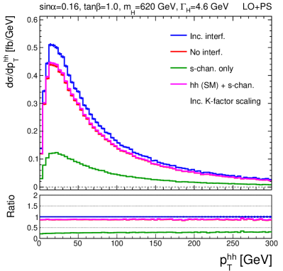
Figure 19: The di-Higgs $p_{\mathrm{T}}$ distributions for BM1 before (left) and after (right) experimental smearing. The blue lines show the full di-Higgs spectrum including all interference terms. This is compared to the spectrum excluding the $\mathrm{S_{H}}{\text{-}}\Box$ and $\mathrm{S_{H}}{\text{-}}\mathrm{S_{h}}$ interference terms shown in red, the $H$ $s$-channel spectrum ($\mathrm{S_{H}}$) shown in green, and the incoherent sum of $\mathrm{S_{H}}$ and the SM di-Higgs spectrum in magenta.

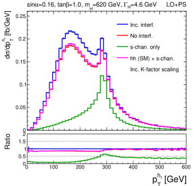
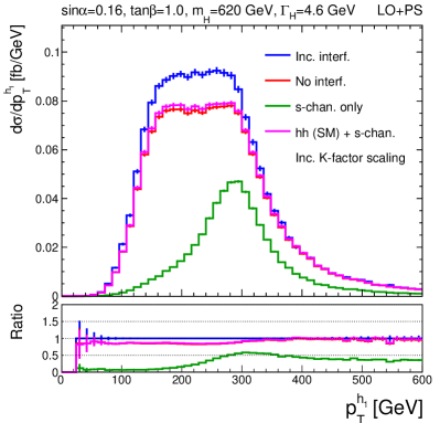
Figure 20: The leading $h$ $p_{\mathrm{T}}$ for BM1 before (left) and after (right) experimental smearing. The blue lines show the full di-Higgs spectrum including all interference terms. This is compared to the spectrum excluding the $\mathrm{S_{H}}{\text{-}}\Box$ and $\mathrm{S_{H}}{\text{-}}\mathrm{S_{h}}$ interference terms shown in red, the $H$ $s$-channel spectrum ($\mathrm{S_{H}}$) shown in green, and the incoherent sum of $\mathrm{S_{H}}$ and the SM di-Higgs spectrum in magenta.

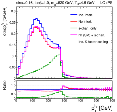
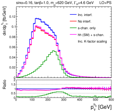
Figure 21: The sub-leading $h$ $p_{\mathrm{T}}$ before (left) and after (right) experimental smearing. The blue lines show the full di-Higgs spectrum including all interference terms. This is compared to the spectrum excluding the $\mathrm{S_{H}}{\text{-}}\Box$ and $\mathrm{S_{H}}{\text{-}}\mathrm{S_{h}}$ interference terms shown in red, the $H$ $s$-channel spectrum ($\mathrm{S_{H}}$) shown in green, and the incoherent sum of $\mathrm{S_{H}}$ and the SM di-Higgs spectrum in magenta.

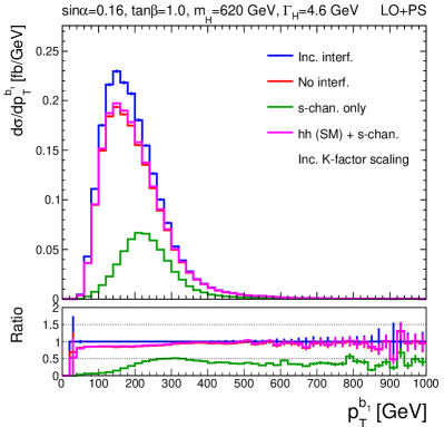
Figure 22: The $p_{\mathrm{T}}$ of the leading $b$-jet before (left) and after (right) experimental smearing. The blue lines show the full di-Higgs spectrum including all interference terms. This is compared to the spectrum excluding the $\mathrm{S_{H}}{\text{-}}\Box$ and $\mathrm{S_{H}}{\text{-}}\mathrm{S_{h}}$ interference terms shown in red, the $H$ $s$-channel spectrum ($\mathrm{S_{H}}$) shown in green, and the incoherent sum of $\mathrm{S_{H}}$ and the SM di-Higgs spectrum in magenta. No $p_{\mathrm{T}}$ or $\mathrm{H}_{\mathrm{T}}$ cuts have been applied for the smeared distributions in this case.

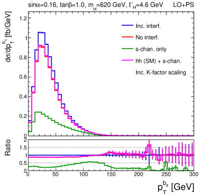
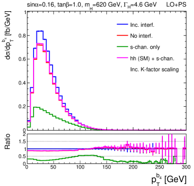
Figure 23: The $p_{\mathrm{T}}$ of the softest $b$-jet before (left) and after (right) experimental smearing. The blue lines show the full di-Higgs spectrum including all interference terms. This is compared to the spectrum excluding the $\mathrm{S_{H}}{\text{-}}\Box$ and $\mathrm{S_{H}}{\text{-}}\mathrm{S_{h}}$ interference terms shown in red, the $H$ $s$-channel spectrum ($\mathrm{S_{H}}$) shown in green, and the incoherent sum of $\mathrm{S_{H}}$ and the SM di-Higgs spectrum in magenta. No $p_{\mathrm{T}}$ or $\mathrm{H}_{\mathrm{T}}$ cuts have been applied for the smeared distributions in this case.

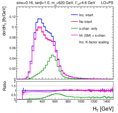
Figure 24: The $\mathrm{H}_{\mathrm{T}}$ of the $b$-jets before (left) and after (right) experimental smearing. The blue lines show the full di-Higgs spectrum including all interference terms. This is compared to the spectrum excluding the $\mathrm{S_{H}}{\text{-}}\Box$ and $\mathrm{S_{H}}{\text{-}}\mathrm{S_{h}}$ interference terms shown in red, the $H$ $s$-channel spectrum ($\mathrm{S_{H}}$) shown in green, and the incoherent sum of $\mathrm{S_{H}}$ and the SM di-Higgs spectrum in magenta. No $p_{\mathrm{T}}$ or $\mathrm{H}_{\mathrm{T}}$ cuts have been applied for the smeared distributions in this case.

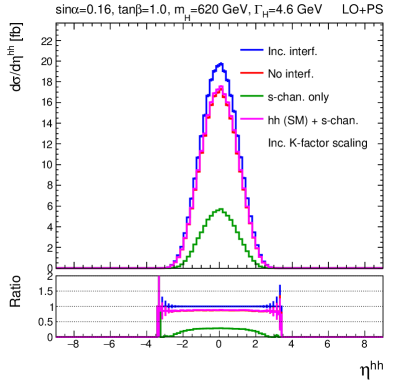
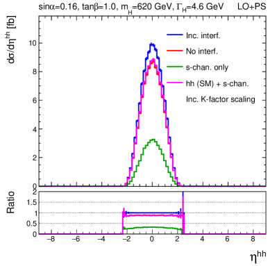
Figure 25: The di-Higgs $\eta$ distributions for BM1 before (left) and after (right) experimental smearing. The blue lines show the full di-Higgs spectrum including all interference terms. This is compared to the spectrum excluding the $\mathrm{S_{H}}{\text{-}}\Box$ and $\mathrm{S_{H}}{\text{-}}\mathrm{S_{h}}$ interference terms shown in red, the $H$ $s$-channel spectrum ($\mathrm{S_{H}}$) shown in green, and the incoherent sum of $\mathrm{S_{H}}$ and the SM di-Higgs spectrum in magenta.

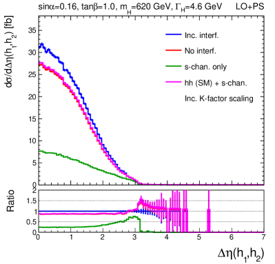
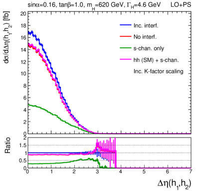
Figure 26: The $\Delta\eta$ between the two $h$ for BM1 before (left) and after (right) experimental smearing. The blue lines show the full di-Higgs spectrum including all interference terms. This is compared to the spectrum excluding the $\mathrm{S_{H}}{\text{-}}\Box$ and $\mathrm{S_{H}}{\text{-}}\mathrm{S_{h}}$ interference terms shown in red, the $H$ $s$-channel spectrum ($\mathrm{S_{H}}$) shown in green, and the incoherent sum of $\mathrm{S_{H}}$ and the SM di-Higgs spectrum in magenta.

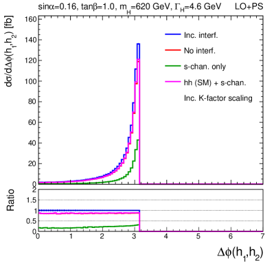
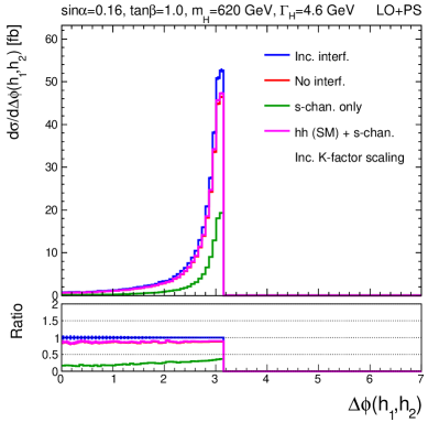
Figure 27: The $\Delta\phi$ between the two $h$ before (left) and after (right) experimental smearing. The blue lines show the full di-Higgs spectrum including all interference terms. This is compared to the spectrum excluding the $\mathrm{S_{H}}{\text{-}}\Box$ and $\mathrm{S_{H}}{\text{-}}\mathrm{S_{h}}$ interference terms shown in red, the $H$ $s$-channel spectrum ($\mathrm{S_{H}}$) shown in green, and the incoherent sum of $\mathrm{S_{H}}$ and the SM di-Higgs spectrum in magenta.

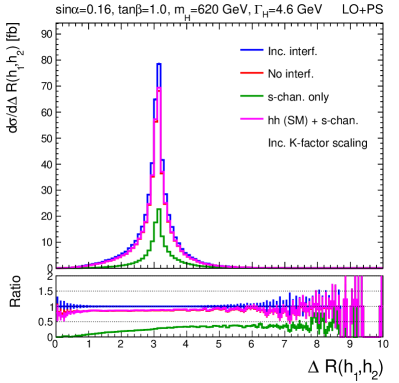
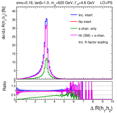
Figure 28: The $\Delta R$ between the two $h$ before (left) and after (right) experimental smearing. The blue lines show the full di-Higgs spectrum including all interference terms. This is compared to the spectrum excluding the $\mathrm{S_{H}}{\text{-}}\Box$ and $\mathrm{S_{H}}{\text{-}}\mathrm{S_{h}}$ interference terms shown in red, the $H$ $s$-channel spectrum ($\mathrm{S_{H}}$) shown in green, and the incoherent sum of $\mathrm{S_{H}}$ and the SM di-Higgs spectrum in magenta.

VII.2 BM2 and BM3

We define two BM points, BM2 and BM3, to investigate scenarios where the interference may affect the shapes of the distributions without necessarily changing the total cross-section. BM2 is taken as the point with the largest value of $\left(\Delta\sigma\right)_{\text{rel}}^{\sum}$ (equal to 29.0%), which is found for $m_{H}=440\,{\,\rm GeV}$, $\sin\alpha=0.16$, and $\tan\beta=0.5$. We define BM3 by additionally requiring $\left(\Delta\sigma\right)_{\text{rel}}<1\%$ when determining the maximum $\left(\Delta\sigma\right)_{\text{rel}}^{\sum}$ value. This allows us to explicitly select a scenario where the effect on the total cross-section is negligible. The values of $\left(\Delta\sigma\right)_{\text{rel}}^{\sum}$ and $\left(\Delta\sigma\right)_{\text{rel}}$ in this scenario are 24.5% and -0.8%, respectively. For comparison, the value of $\left(\Delta\sigma\right)_{\text{rel}}$ in BM2 is 6.0%. The values of the model parameters for this scenario are $m_{H}=380\,{\,\rm GeV}$, $\sin\alpha=0.16$, and $\tan\beta=0.5$.

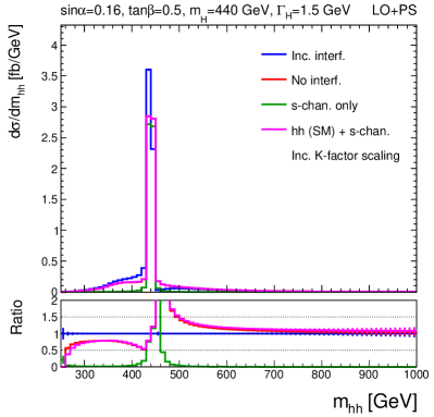
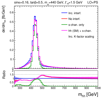
Figure 29: The di-Higgs mass distributions for BM2 before (left) and after (right) experimental smearing. The blue lines show the full di-Higgs spectrum including all interference terms. This is compared to the spectrum excluding the $\mathrm{S_{H}}{\text{-}}\Box$ and $\mathrm{S_{H}}{\text{-}}\mathrm{S_{h}}$ interference terms shown in red, the $H$ $s$-channel spectrum ($\mathrm{S_{H}}$) shown in green, and the incoherent sum of $\mathrm{S_{H}}$ and the SM di-Higgs spectrum in magenta.

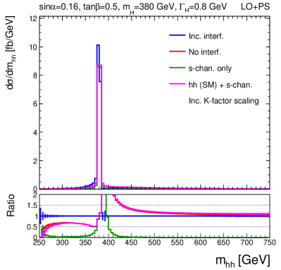
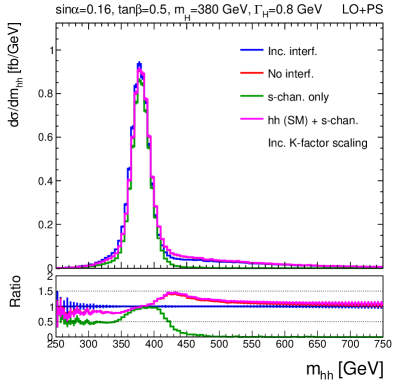
Figure 30: The di-Higgs mass distributions for BM3 before (left) and after (right) experimental smearing. The blue lines show the full di-Higgs spectrum including all interference terms. This is compared to the spectrum excluding the $\mathrm{S_{H}}{\text{-}}\Box$ and $\mathrm{S_{H}}{\text{-}}\mathrm{S_{h}}$ interference terms shown in red, the $H$ $s$-channel spectrum ($\mathrm{S_{H}}$) shown in green, and the incoherent sum of $\mathrm{S_{H}}$ and the SM di-Higgs spectrum in magenta.

The $m_{hh}$ distributions for BM2 and BM3 are shown in Figures 29 and 30, respectively. In general, the effect of the interference in these BMs is visibly smaller than for BM1, especially after the experimental smearing is applied. However, comparing the ratios in the figures we observe that the relative differences away from the resonant peak are actually quite similar to BM1, but as the relative contribution of the non-resonant component compared to the $\mathrm{S_{H}}$ contribution is smaller the effect is less noticeable.

For BM3, we observe only a small impact from neglecting the interference, and even the $\mathrm{S_{H}}$-only assumption is fairly close to the full distribution in this case. This is somewhat expected since the non-resonant contribution compared to the $\mathrm{S_{H}}$ component is small in this scenario and so the $\left(\Delta\sigma\right)_{\text{rel}}<1\%$ requirement imposed when selecting the point means that the interference manifests almost exclusively as a shift in the position of the resonant peak. The experimental smearing then largely washes out this shift reducing the impact of the interference on the distribution.

Since it is possible that the experimental collaborations could improve the $m_{hh}$ resolution in the future, we investigated if such an improvement would significantly change the conclusion drawn in this case. To this end, we artificially improved the $m_{hh}$ resolution by a factor of two and display the resulting $m_{hh}$ distribution in Figure 31. In this case, we observe a slightly larger difference between the full spectrum and the no-interference scenario.

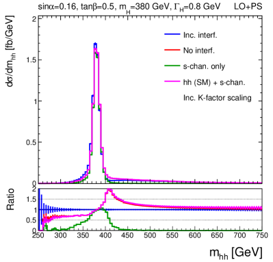
Figure 31: The di-Higgs mass distributions for BM3 after experimental smearing while artificially improving the $m_{hh}$ resolution by a factor of two compared to Figure 30. The blue lines show the full di-Higgs spectrum including all interference terms. This is compared to the spectrum excluding the $\mathrm{S_{H}}{\text{-}}\Box$ and $\mathrm{S_{H}}{\text{-}}\mathrm{S_{h}}$ interference terms shown in red, the $H$ $s$-channel spectrum ($\mathrm{S_{H}}$) shown in green, and the incoherent sum of $\mathrm{S_{H}}$ and the SM di-Higgs spectrum in magenta.

VII.3 BM4 and BM5

We define two BM points, BM4 and BM5, to investigate scenarios where the non-resonant contribution to the di-Higgs spectrum is significant, independent of the interference. These BMs are selected by looking for the points where the relative fraction of non-resonant events close to the resonant peak is maximal. The fraction is defined as $f=\frac{\sigma_{\mathrm{woH}}}{\sigma_{\mathrm{S_{H}}}+\sigma_{\mathrm{woH}}}$, where $\sigma_{\mathrm{woH}}$ is the cross-section for the $\Box+\mathrm{S_{h}}+\mathrm{S_{h}}{\text{-}}\Box$ process requiring $0.9<\frac{m_{hh}^{\mathrm{truth}}}{m_{H}}<1.1$ to select events with $\pm 10\%$ of $m_{H}$. This definition thus ignores the effect of the interference of the $H$ with the non-resonant terms. Two BMs are defined, since the scan returns different points depending on whether we use $L=400~{}\mathrm{fb}^{-1}$ or $L=3000~{}\mathrm{fb}^{-1}$. BM4 was found for the $L=400~{}\mathrm{fb}^{-1}$ scan which has $f=28.8\%$. The model parameters are $m_{H}=560\,{\,\rm GeV}$, $\sin\alpha=-0.16$, and $\tan\beta=0.5$. BM5 was defined for the $L=3000~{}\mathrm{fb}^{-1}$ which estimates $f=54.5\%$. The model parameters in the case are $m_{H}=500\,{\,\rm GeV}$, $\sin\alpha=0.08$, and $\tan\beta=0.5$.

Figures 32 and 33 show the $m_{hh}$ distributions in BM4 and BM5, respectively. In both cases there is a significant difference between the $\mathrm{S_{H}}$-only assumption and both the full model and no-interference scenarios. BM4 also shows a sizeable effect due to the interference. In contrast, the impact of the interference in BM5 is quite small. However, the non-resonant contribution is even more significant in this case and it clearly has to be taken into account by future experimental searches.

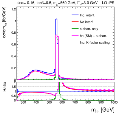
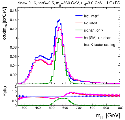
Figure 32: The di-Higgs mass distributions for BM4 before (left) and after (right) experimental smearing. The blue lines show the full di-Higgs spectrum including all interference terms. This is compared to the spectrum excluding the $\mathrm{S_{H}}{\text{-}}\Box$ and $\mathrm{S_{H}}{\text{-}}\mathrm{S_{h}}$ interference terms shown in red, the $H$ $s$-channel spectrum ($\mathrm{S_{H}}$) shown in green, and the incoherent sum of $\mathrm{S_{H}}$ and the SM di-Higgs spectrum in magenta.

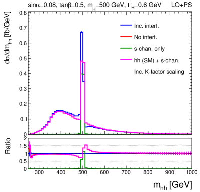
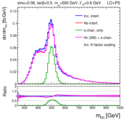
Figure 33: The di-Higgs mass distributions for BM5 before (left) and after (right) experimental smearing. The blue lines show the full di-Higgs spectrum including all interference terms. This is compared to the spectrum excluding the $\mathrm{S_{H}}{\text{-}}\Box$ and $\mathrm{S_{H}}{\text{-}}\mathrm{S_{h}}$ interference terms shown in red, the $H$ $s$-channel spectrum ($\mathrm{S_{H}}$) shown in green, and the incoherent sum of $\mathrm{S_{H}}$ and the SM di-Higgs spectrum in magenta.

VII.4 BM6 and BM7

We define two BM points to study the interference effects for large values of $m_{H}$. We define the BMs, BM6 and BM7, as the points with maximal values of $m_{H}$ within reach of the LHC for $L=400~{}\mathrm{fb}^{-1}$ and $L=3000~{}\mathrm{fb}^{-1}$, respectively. BM6 was found for $m_{H}=680\,{\,\rm GeV}$, $\sin\alpha=0.16$, and $\tan\beta=1.0$. The model parameters for BM7 are $m_{H}=870\,{\,\rm GeV}$, $\sin\alpha=0.15$, and $\tan\beta=1.1$.

The $m_{hh}$ distributions are shown in Figures 34 and 35. Both BMs predict a more sizeable contribution to the total di-Higgs spectrum from the non-resonant contribution compared to $\mathrm{S_{H}}$. However, we note that, as the resonant part peaks at higher mass, it may still drive the sensitivity for the experimental searches, as the backgrounds are probably also small for large $m_{hh}$. Once again, these distributions underline the need to take the non-resonant contributions into account in the experimental searches.

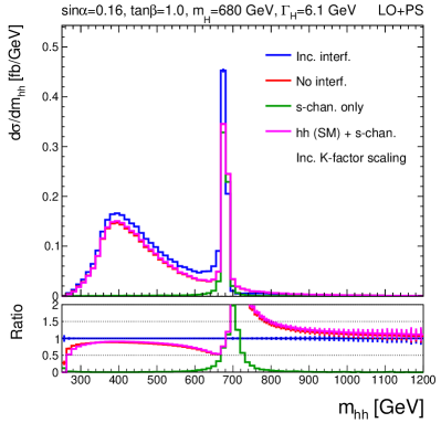
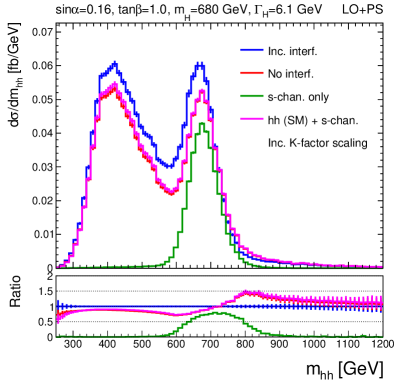
Figure 34: The di-Higgs mass distributions for BM6 before (left) and after (right) experimental smearing. The blue lines show the full di-Higgs spectrum including all interference terms. This is compared to the spectrum excluding the $\mathrm{S_{H}}{\text{-}}\Box$ and $\mathrm{S_{H}}{\text{-}}\mathrm{S_{h}}$ interference terms shown in red, the $H$ $s$-channel spectrum ($\mathrm{S_{H}}$) shown in green, and the incoherent sum of $\mathrm{S_{H}}$ and the SM di-Higgs spectrum in magenta.

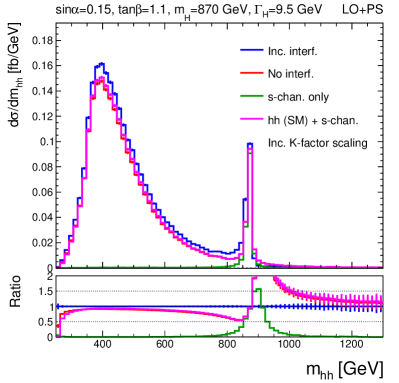
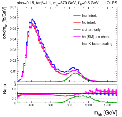
Figure 35: The di-Higgs mass distributions for BM7 before (left) and after (right) experimental smearing. The blue lines show the full di-Higgs spectrum including all interference terms. This is compared to the spectrum excluding the $\mathrm{S_{H}}{\text{-}}\Box$ and $\mathrm{S_{H}}{\text{-}}\mathrm{S_{h}}$ interference terms shown in red, the $H$ $s$-channel spectrum ($\mathrm{S_{H}}$) shown in green, and the incoherent sum of $\mathrm{S_{H}}$ and the SM di-Higgs spectrum in magenta.

VII.5 BM8

BM8 is defined as the point which has the largest deviation of $\lambda_{hhh}$ from the SM value at LO. This main purpose of this BM is to investigate whether or not assuming SM-like couplings for the non-resonant contribution is a reasonable approximation. This may have practical implications for experimental searches, i.e. fixing these couplings to SM values reduces the dimensionality of the parameter space that needs to be scanned. The largest deviation for $\lambda_{hhh}$ is found for $m_{H}=260\,{\,\rm GeV}$, $\sin\alpha=0.24$, and $\tan\beta=3.5$ which yields a value of $\kappa_{\lambda_{hhh}}=0.87$.

The $m_{hh}$ distributions are shown in Figure 36. We observe no major differences between the no-interference and SM+$\mathrm{S_{H}}$ distributions, implying that assuming SM couplings for the $h$ is a reasonable assumption in this case. The non-resonant contribution to the spectrum is less noticeable in these plots as the resonant $\mathrm{S_{H}}$ peak is large. To study in more detail how the values of the $h$ couplings influence the non-resonant contribution, we remove the $\mathrm{S_{H}}$, $\mathrm{S_{H}}{\text{-}}\Box$, and $\mathrm{S_{H}}{\text{-}}\mathrm{S_{h}}$ contributions to the spectrum, as shown in Figure 37. The non-resonant spectrum for BM8 shown in blue is compared to the SM shown in red. We see only small differences between the two distributions, mainly impacting the low $m_{hh}$ bins where the event yield is low. The differences in the distributions are somewhat smaller than one might expect given that $\kappa_{\lambda_{hhh}}$ deviates from the SM value by a non-negligible amount. This is due to a small deviation in the value of $\kappa_{q}^{h}$, which is equal to 0.97 in this BM. This causes an accidental cancellation between the $\Box$ and $\mathrm{S_{h}}$ components, which decrease in size for couplings $<1$, and the $\mathrm{S_{h}}{\text{-}}\Box$ component which increases due to the destructive nature of the interference. The scenario where only $\kappa_{\lambda_{hhh}}$ deviates from the SM and $\kappa_{q}^{h}=1$ is shown in green in the Figure for comparison. Even in this scenario the deviation in the non-resonant yield is only $\approx 10\%$ so it is unlikely that the LHC experiments will be sensitive to the deviations in $\kappa_{\lambda_{hhh}}$ in this model.

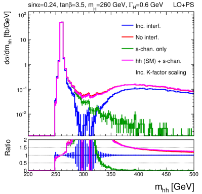
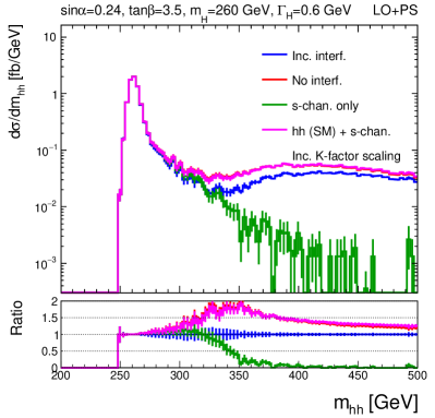
Figure 36: The di-Higgs mass distributions for BM8 before (left) and after (right) experimental smearing. The blue lines show the full di-Higgs spectrum including all interference terms. This is compared to the spectrum excluding the $\mathrm{S_{H}}{\text{-}}\Box$ and $\mathrm{S_{H}}{\text{-}}\mathrm{S_{h}}$ interference terms shown in red, the $H$ $s$-channel spectrum ($\mathrm{S_{H}}$) shown in green, and the incoherent sum of $\mathrm{S_{H}}$ and the SM di-Higgs spectrum in magenta.

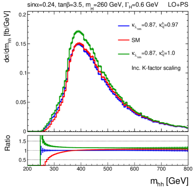
Figure 37: The non-resonant contributions to the di-Higgs mass spectrum for BM8 before experimental smearing. The blue line shows the case where both $\kappa_{\lambda_{hhh}}$ and $\kappa_{q}^{h}$ are set to the values predicted in BM8 ($\kappa_{\lambda_{hhh}}=0.87$, $\kappa_{q}^{h}=0.97$). This is compared to the SM spectrum shown in red and the spectrum when $\kappa_{q}^{h}$ is set to the SM value and $\kappa_{\lambda_{hhh}}=0.87$ shown in green.

VII.6 BM9

The final BM, BM9, is defined as the point which has the largest value of $\frac{\Gamma_{H}}{m_{H}}$, which is found for $m_{H}=800\,{\,\rm GeV}$, $\sin\alpha=0.16$, and $\tan\beta=1.0$. The value of $\frac{\Gamma_{H}}{m_{H}}$ is 1.2%. The $m_{hh}$ distributions are shown in Figures 38.

The main purpose of this BM is to investigate whether finite width effects may invalidate the procedure followed by several experimental searches whereby a narrow width is assumed for the generated $H$ signal. To investigate this question, we display the $m_{hh}$ distributions for the $\mathrm{S_{H}}$ contribution in Figure 39. The figure compares the $m_{hh}$ distributions predicted for samples generated with the correct width to samples generated assuming a narrow-width of $20\,{\rm MeV}$. For the latter, the sample yield is scaled by $(20\,{\rm MeV})/\Gamma_{H}$ to account for the different branching fractions. The distributions are shown for our nominal assumption about the experimental resolution (left plot) and a more optimistic experimental resolution, which is improved by a factor of two (right plot).

The $m_{hh}$ distributions obtained for the nominal smearing are in quite good agreement. The difference between the two distributions is only around 7% at the maximum of the peak, and thus the experiments would probably not be able to resolve the differences. The optimistic scenario is intended to investigate the impact of potential future improvements to the experimental resolution if the experimental collaborations are able to improve the $m_{hh}$ resolution in the future and/or if a channel with a better resolution is used instead (e.g. $bb\gamma\gamma$). As expected, when the resolution is bettered the experiments become more sensitive to the width effects, and the difference between the $m_{hh}$ distributions can be as large as 14% at the maximum of the peak. While this may lead to small modifications to the measured experimental limits, it would probably not significantly alter the overall conclusions of the searches and thus we conclude that the narrow-width assumption for generation of the $\mathrm{S_{H}}$ contributions is a reasonable approximation for the singlet model. However, we stress that this conclusion is specific to the singlet model since other beyond the SM scenarios can still accommodate more sizeable widths $\mathcal{O}(10\%)$, and these scenarios will require a proper treatment of finite width effects. It is also important to stress that, while the finite width effects for the $\mathrm{S_{H}}$-only process can be accounted for via the branching fraction rescaling, this is not possible for the $\mathrm{S_{H}}{\text{-}}\Box$ and $\mathrm{S_{H}}{\text{-}}\mathrm{S_{h}}$ interference terms. As demonstrated previously in Figure 9, the width modifies these distributions in a non-trivial way (e.g. differentially in $m_{hh}$), and thus it is not possible to account for this by the application of a constant scale factor as for the $\mathrm{S_{H}}$ contribution.

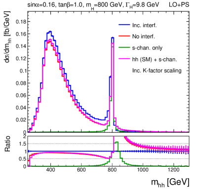
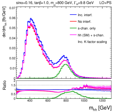
Figure 38: The di-Higgs mass distributions for BM9 before (left) and after (right) experimental smearing. The blue lines show the full di-Higgs spectrum including all interference terms. This is compared to the spectrum excluding the $\mathrm{S_{H}}{\text{-}}\Box$ and $\mathrm{S_{H}}{\text{-}}\mathrm{S_{h}}$ interference terms shown in red, the $H$ $s$-channel spectrum ($\mathrm{S_{H}}$) shown in green, and the incoherent sum of $\mathrm{S_{H}}$ and the SM di-Higgs spectrum in magenta.

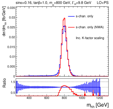
Figure 39: The di-Higgs mass distributions for BM9 after experimental smearing are displayed for the $s$-channel only ($\mathrm{S_{H}}$) contributions. The blue lines show distributions obtained using the correct width ($\Gamma_{H}=9.8\,{\,\rm GeV}$), while the red lines display the distributions obtained using the NWA with $\Gamma_{H}=20\,{\rm MeV}$ and rescaling the the branching fractions by $(20\,{\rm MeV})/\Gamma_{H}$ as described in the text. The left plot shows the distributions for the nominal assumed experimental resolution while the right plot shows the distributions after artificially improving the $m_{hh}$ resolution by a factor of two.

VIII Summary

We have presented the latest experimental and theoretical limits on the parameter space of the real singlet extension of the SM Higgs sector. The tightest bounds on the model at high $m_{H}$ come from the measurements of the $W$-boson mass, whereas the bounds at low $\sin\alpha$ are driven by direct searches for $H\rightarrow VV/hh$ at the LHC.

We have investigated in detail interference effects between resonant and non-resonant contributions, where the former originates from the production of a heavy additional Higgs boson which subsequently decays into two lighter SM-like Higgs bosons ($H\rightarrow hh$). We have studied various kinematic observables, such as the commonly investigated di-Higgs invariant mass ($m_{hh}$), as well as a number of other variables that are relevant for the respective experimental searches. In particular, we find that the transverse momenta of the two SM-like Higgs bosons have a comparable sensitivity to interference effects.

We have identified regions of the parameter space where interference effects between the non-resonant and resonant diagrams are sizeable. In order to account for NLO kinematics as well as interference effects, we have proposed a prescription that includes both, where we find good agreement with the correct NLO description when available. Using our methodology, we have defined benchmark scenarios exhibiting interesting features of the model. For several benchmarks scenarios, we find that the contribution of the non-resonant di-Higgs diagrams is significant and in some cases even dwarfs the resonant component. We have also observed that interference effects have a non-negligible effect on both the cross-sections and differential distributions. We strongly encourage the experimental collaborations to take these effects into account in future searches for additional Higgs bosons. Furthermore, the correct physical prediction of the total width needs to be used in realistic simulation as the width can crucially impact the rates as well as the relevance of the interference term. Finally, we have presented a publicly available tool, HHReweighter reweight_repo , for performing matrix-element reweighting that allows such interference effects to be taken into account in a computationally efficient way.

Appendix A Interference evaluation in an additional observable

In Figure A.1, we display the differential distribution in $\Delta\phi_{hh}$ for both parameter points discussed in Section V.1. The similarity of the blue line (coherent sum of all contributions to $pp\to hh$) and the green line (incoherent sum of the contributions via $H$ and without $H$, i.e. without the interference term) indicates that the interference does not contribute significantly to this variable.

(a)

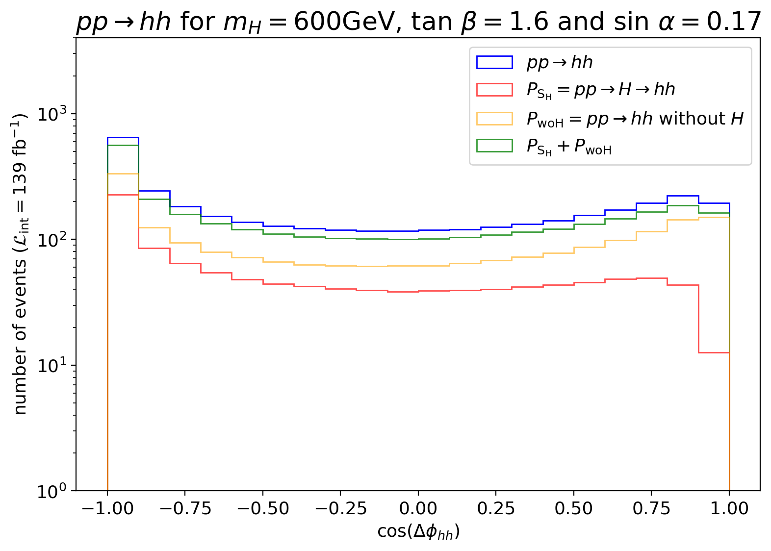
(b)

(c)

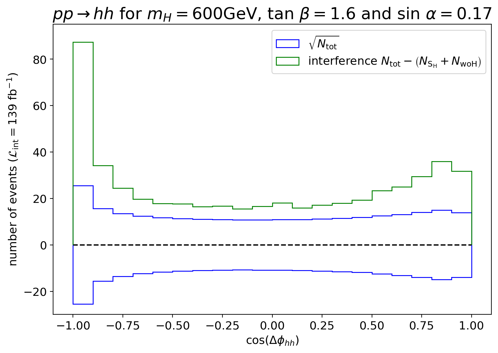
(d)

Figure A.1: Upper row: the angle between the Higgs bosons $\Delta\phi_{hh}$ with $P_{\text{tot}}$ (blue), $P_{\mathrm{S_{H}}}$ (red), $P_{\text{woH}}$ (orange) and the sum of $P_{\mathrm{S_{H}}}$ and $P_{\text{woH}}$ (green). The difference between the blue and the green line corresponds to the interference term. Lower row: the interference for the two respective parameter points (left column vs. right column).

Appendix B Additional validation plots of the reweighting method

The reweighting method described in Section VI is validated for all benchmark points given in Section VII. Figures B.1–B.3 show the reweighted $m_{hh}$ distribution (blue) compared to the $m_{hh}$ distribution obtained from a MC sample generated directly for the target model parameters (black).

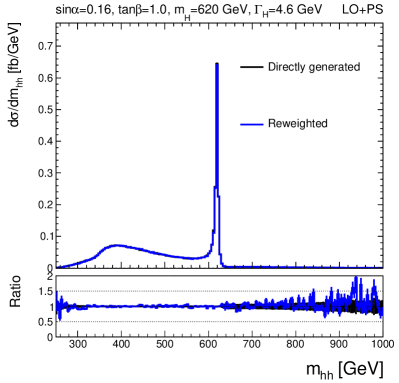
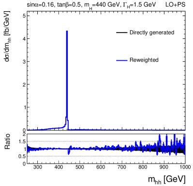
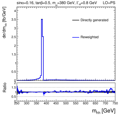
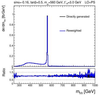
Figure B.1: The reweighting method is validating by comparing reweighted di-Higgs mass distribution (blue) to the distribution obtained by directly simulating the di-Higgs events for a set of parameter points (black). The distributions are shown for BM1 (upper left), BM2 (upper right), BM3 (lower left) and BM4 (lower right).

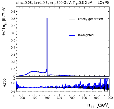
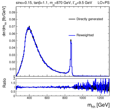
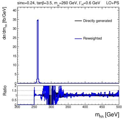
Figure B.2: The reweighting method is validating by comparing reweighted di-Higgs mass distribution (blue) to the distribution obtained by directly simulating the di-Higgs events for a set of parameter points (black). The distributions are shown for BM5 (upper left), BM6 (upper right), BM7 (lower left) and BM8 (lower right).

Figure B.3: The reweighting method is validating by comparing reweighted di-Higgs mass distribution (blue) to the distribution obtained by directly simulating the di-Higgs events for a set of parameter points (black). The distribution is shown for BM9.

References

- (1) T. Robens and T. Stefaniak, Status of the Higgs Singlet Extension of the Standard Model after LHC Run 1, Eur. Phys. J. C 75 (2015) 104 [1501.02234].
- (2) T. Robens and T. Stefaniak, LHC Benchmark Scenarios for the Real Higgs Singlet Extension of the Standard Model, Eur. Phys. J. C 76 (2016) 268 [1601.07880].
- (3) T. Robens, Constraining Extended Scalar Sectors at Current and Future Colliders—An Update, Springer Proc. Phys. 292 (2023) 141 [2209.15544].
- (4) J. Alison et al., Higgs boson potential at colliders: Status and perspectives, Rev. Phys. 5 (2020) 100045 [1910.00012].
- (5) V. Brigljevic et al., HHH Whitepaper, in HHH Workshop, 7, 2024 [2407.03015].
- (6) S. Dawson and I.M. Lewis, NLO corrections to double Higgs boson production in the Higgs singlet model, Phys. Rev. D 92 (2015) 094023 [1508.05397].
- (7) S. Dawson and I.M. Lewis, Singlet Model Interference Effects with High Scale UV Physics, Phys. Rev. D 95 (2017) 015004 [1605.04944].
- (8) I.M. Lewis and M. Sullivan, Benchmarks for Double Higgs Production in the Singlet Extended Standard Model at the LHC, Phys. Rev. D 96 (2017) 035037 [1701.08774].
- (9) M. Carena, Z. Liu and M. Riembau, Probing the electroweak phase transition via enhanced di-Higgs boson production, Phys. Rev. D 97 (2018) 095032 [1801.00794].
- (10) P. Basler, S. Dawson, C. Englert and M. Mühlleitner, Di-Higgs boson peaks and top valleys: Interference effects in Higgs sector extensions, Phys. Rev. D 101 (2020) 015019 [1909.09987].
- (11) S. Heinemeyer, M. Mühlleitner, K. Radchenko and G. Weiglein, Higgs Pair Production in the 2HDM: Impact of Loop Corrections to the Trilinear Higgs Couplings and Interference Effects on Experimental Limits, 2403.14776.
- (12) R.K. Ellis, W.J. Stirling and B.R. Webber, QCD and collider physics, vol. 8, Cambridge University Press (2, 2011), 10.1017/CBO9780511628788.
- (13) J. Campbell, J. Huston and F. Krauss, The Black Book of Quantum Chromodynamics : a Primer for the LHC Era, Oxford University Press (2018), 10.1093/oso/9780199652747.001.0001.
- (14) J.F. Gunion, H.E. Haber and J. Wudka, Sum rules for Higgs bosons, Phys. Rev. D 43 (1991) 904.
- (15) ATLAS collaboration, Combination of Searches for Higgs Boson Pair Production in pp Collisions at s=13 TeV with the ATLAS Detector, Phys. Rev. Lett. 133 (2024) 101801 [2406.09971].
- (16) CMS collaboration, Searches for Higgs boson production through decays of heavy resonances, 2403.16926.
- (17) A. Carvalho, M. Dall’Osso, T. Dorigo, F. Goertz, C.A. Gottardo and M. Tosi, Higgs Pair Production: Choosing Benchmarks With Cluster Analysis, JHEP 04 (2016) 126 [1507.02245].
- (18) G. Buchalla, M. Capozi, A. Celis, G. Heinrich and L. Scyboz, Higgs boson pair production in non-linear Effective Field Theory with full -dependence at NLO QCD, JHEP 09 (2018) 057 [1806.05162].
- (19) M. Capozi and G. Heinrich, Exploring anomalous couplings in Higgs boson pair production through shape analysis, JHEP 03 (2020) 091 [1908.08923].
- (20) L. Alasfar et al., Effective Field Theory descriptions of Higgs boson pair production, 2304.01968.
- (21) R.M. Schabinger and J.D. Wells, A Minimal spontaneously broken hidden sector and its impact on Higgs boson physics at the large hadron collider, Phys. Rev. D 72 (2005) 093007 [hep-ph/0509209].
- (22) D. O’Connell, M.J. Ramsey-Musolf and M.B. Wise, Minimal Extension of the Standard Model Scalar Sector, Phys. Rev. D 75 (2007) 037701 [hep-ph/0611014].
- (23) B. Patt and F. Wilczek, Higgs-field portal into hidden sectors, hep-ph/0605188.
- (24) V. Barger, P. Langacker, M. McCaskey, M.J. Ramsey-Musolf and G. Shaughnessy, LHC Phenomenology of an Extended Standard Model with a Real Scalar Singlet, Phys. Rev. D 77 (2008) 035005 [0706.4311].
- (25) M. Bowen, Y. Cui and J.D. Wells, Narrow trans-TeV Higgs bosons and H — hh decays: Two LHC search paths for a hidden sector Higgs boson, JHEP 03 (2007) 036 [hep-ph/0701035].
- (26) P. Huang, A.J. Long and L.-T. Wang, Probing the Electroweak Phase Transition with Higgs Factories and Gravitational Waves, Phys. Rev. D 94 (2016) 075008 [1608.06619].
- (27) S. Dawson and C.W. Murphy, Standard Model EFT and Extended Scalar Sectors, Phys. Rev. D 96 (2017) 015041 [1704.07851].
- (28) A. Ilnicka, T. Robens and T. Stefaniak, Constraining Extended Scalar Sectors at the LHC and beyond, Mod. Phys. Lett. A 33 (2018) 1830007 [1803.03594].
- (29) B. Heinemann and Y. Nir, The Higgs program and open questions in particle physics and cosmology, Usp. Fiz. Nauk 189 (2019) 985 [1905.00382].
- (30) E. Fuchs, O. Matsedonskyi, I. Savoray and M. Schlaffer, Collider searches for scalar singlets across lifetimes, JHEP 04 (2021) 019 [2008.12773].
- (31) D. López-Val and T. Robens, r and the W-boson mass in the singlet extension of the standard model, Phys. Rev. D 90 (2014) 114018 [1406.1043].
- (32) A. Papaefstathiou, T. Robens and G. White, Signal strength and W-boson mass measurements as a probe of the electro-weak phase transition at colliders - Snowmass White Paper, in Snowmass 2021, 5, 2022 [2205.14379].
- (33) H. Bahl, T. Biekötter, S. Heinemeyer, C. Li, S. Paasch, G. Weiglein et al., HiggsTools: BSM scalar phenomenology with new versions of HiggsBounds and HiggsSignals, Comput. Phys. Commun. 291 (2023) 108803 [2210.09332].
- (34) P. Bechtle, O. Brein, S. Heinemeyer, G. Weiglein and K.E. Williams, HiggsBounds: Confronting Arbitrary Higgs Sectors with Exclusion Bounds from LEP and the Tevatron, Comput. Phys. Commun. 181 (2010) 138 [0811.4169].
- (35) P. Bechtle, O. Brein, S. Heinemeyer, G. Weiglein and K.E. Williams, HiggsBounds 2.0.0: Confronting Neutral and Charged Higgs Sector Predictions with Exclusion Bounds from LEP and the Tevatron, Comput. Phys. Commun. 182 (2011) 2605 [1102.1898].
- (36) P. Bechtle, O. Brein, S. Heinemeyer, O. Stål, T. Stefaniak, G. Weiglein et al., : Improved Tests of Extended Higgs Sectors against Exclusion Bounds from LEP, the Tevatron and the LHC, Eur. Phys. J. C 74 (2014) 2693 [1311.0055].
- (37) P. Bechtle, D. Dercks, S. Heinemeyer, T. Klingl, T. Stefaniak, G. Weiglein et al., HiggsBounds-5: Testing Higgs Sectors in the LHC 13 TeV Era, Eur. Phys. J. C 80 (2020) 1211 [2006.06007].
- (38) P. Bechtle, S. Heinemeyer, O. Stål, T. Stefaniak and G. Weiglein, : Confronting arbitrary Higgs sectors with measurements at the Tevatron and the LHC, Eur. Phys. J. C 74 (2014) 2711 [1305.1933].
- (39) P. Bechtle, S. Heinemeyer, O. Stål, T. Stefaniak and G. Weiglein, Probing the Standard Model with Higgs signal rates from the Tevatron, the LHC and a future ILC, JHEP 11 (2014) 039 [1403.1582].
- (40) P. Bechtle, S. Heinemeyer, T. Klingl, T. Stefaniak, G. Weiglein and J. Wittbrodt, HiggsSignals-2: Probing new physics with precision Higgs measurements in the LHC 13 TeV era, Eur. Phys. J. C 81 (2021) 145 [2012.09197].
- (41) CMS collaboration, Search for a new scalar resonance decaying to a pair of Z bosons in proton-proton collisions at TeV, JHEP 06 (2018) 127 [1804.01939].
- (42) ATLAS collaboration, Search for heavy resonances decaying into a pair of Z bosons in the and final states using 139 of proton–proton collisions at TeV with the ATLAS detector, Eur. Phys. J. C 81 (2021) 332 [2009.14791].
- (43) ATLAS collaboration, Combination of searches for heavy resonances decaying into bosonic and leptonic final states using 36 fb-1 of proton-proton collision data at TeV with the ATLAS detector, Phys. Rev. D 98 (2018) 052008 [1808.02380].
- (44) ATLAS collaboration, Search for heavy diboson resonances in semileptonic final states in pp collisions at TeV with the ATLAS detector, Eur. Phys. J. C 80 (2020) 1165 [2004.14636].
- (45) CMS collaboration, Search for a heavy Higgs boson decaying into two lighter Higgs bosons in the bb final state at 13 TeV, JHEP 11 (2021) 057 [2106.10361].
- (46) ATLAS collaboration, Search for Higgs boson pair production in the two bottom quarks plus two photons final state in collisions at TeV with the ATLAS detector, Phys. Rev. D 106 (2022) 052001 [2112.11876].
- (47) ATLAS collaboration, Search for resonant and non-resonant Higgs boson pair production in the decay channel using 13 TeV pp collision data from the ATLAS detector, JHEP 07 (2023) 040 [2209.10910].
- (48) G.M. Pruna and T. Robens, Higgs singlet extension parameter space in the light of the LHC discovery, Phys. Rev. D 88 (2013) 115012 [1303.1150].
- (49) T. Robens, Two-Real-Singlet Model Benchmark Planes – A Moriond Update, in 57th Rencontres de Moriond on QCD and High Energy Interactions, 5, 2023 [2305.08595].
- (50) LHC Higgs Cross Section Working Group collaboration, Handbook of LHC Higgs Cross Sections: 4. Deciphering the Nature of the Higgs Sector, 1610.07922.
- (51) C. Itzykson and J.B. Zuber, Quantum Field Theory, International Series In Pure and Applied Physics, McGraw-Hill, New York (1980).
- (52) A. Denner and S. Dittmaier, Electroweak Radiative Corrections for Collider Physics, Phys. Rept. 864 (2020) 1 [1912.06823].
- (53) H. Pilkuhn, The Interactions of Hadrons, North-Holland Publishing Company (1967).
- (54) D.A. Dicus, E.C.G. Sudarshan and X. Tata, Factorization Theorem for Decaying Spinning Particles, Phys. Lett. B 154 (1985) 79.
- (55) E. Fuchs and G. Weiglein, Breit-Wigner approximation for propagators of mixed unstable states, JHEP 09 (2017) 079 [1610.06193].
- (56) A. Denner, S. Dittmaier, M. Roth and D. Wackeroth, Predictions for all processes e+ e- 4 fermions + gamma, Nucl. Phys. B 560 (1999) 33 [hep-ph/9904472].
- (57) A. Denner, S. Dittmaier, M. Roth and L.H. Wieders, Electroweak corrections to charged-current e+ e- 4 fermion processes: Technical details and further results, Nucl. Phys. B 724 (2005) 247 [hep-ph/0505042].
- (58) A. Denner and S. Dittmaier, The Complex-mass scheme for perturbative calculations with unstable particles, Nucl. Phys. B Proc. Suppl. 160 (2006) 22 [hep-ph/0605312].
- (59) A. Denner and J.-N. Lang, The Complex-Mass Scheme and Unitarity in perturbative Quantum Field Theory, Eur. Phys. J. C 75 (2015) 377 [1406.6280].
- (60) D. Berdine, N. Kauer and D. Rainwater, Breakdown of the Narrow Width Approximation for New Physics, Phys. Rev. Lett. 99 (2007) 111601 [hep-ph/0703058].
- (61) C. Uhlemann, “Narrow-width approximation in the Minimal Supersymmetric Standard Model.” Diploma thesis, Wuerzburg, 2007.
- (62) C.F. Uhlemann and N. Kauer, Narrow-width approximation accuracy, Nucl. Phys. B 814 (2009) 195 [0807.4112].
- (63) G. Cacciapaglia, A. Deandrea and S. De Curtis, Nearby resonances beyond the Breit-Wigner approximation, Phys. Lett. B 682 (2009) 43 [0906.3417].
- (64) E. Fuchs, “Interference effects in new physics processes at the LHC.” PhD Thesis, U. Hamburg 2015, DESY-THESIS-2015-037, 2015.
- (65) E. Fuchs and G. Weiglein, Impact of CP-violating interference effects on MSSM Higgs searches, Eur. Phys. J. C 78 (2018) 87 [1705.05757].
- (66) E. Bagnaschi et al., MSSM Higgs Boson Searches at the LHC: Benchmark Scenarios for Run 2 and Beyond, Eur. Phys. J. C 79 (2019) 617 [1808.07542].
- (67) A.H. Hoang, S. Plätzer, C. Regner and I. Ruffa, Beyond the Narrow-Width Limit for Off-Shell and Boosted Differential Top Quark Decays, in 16th International Workshop on Top Quark Physics, 1, 2024 [2401.05035].
- (68) E. Fuchs, S. Thewes and G. Weiglein, Interference effects in BSM processes with a generalised narrow-width approximation, Eur. Phys. J. C 75 (2015) 254 [1411.4652].
- (69) J. Alwall, R. Frederix, S. Frixione, V. Hirschi, F. Maltoni, O. Mattelaer et al., The automated computation of tree-level and next-to-leading order differential cross sections, and their matching to parton shower simulations, JHEP 07 (2014) 079 [1405.0301].
- (70) A. Papaefstathiou, T. Robens and G. Tetlalmatzi-Xolocotzi, Triple Higgs Boson Production at the Large Hadron Collider with Two Real Singlet Scalars, JHEP 05 (2021) 193 [2101.00037].
- (71) Papaefstathiou, A., “TwoSinglet model file.” https://gitlab.com/apapaefs/twosinglet.
- (72) P. Nason, A new method for combining NLO QCD with shower Monte Carlo algorithms, JHEP 11 (2004) 040 [hep-ph/0409146].
- (73) S. Frixione, P. Nason and C. Oleari, Matching NLO QCD computations with parton shower simulations: the POWHEG method, JHEP 11 (2007) 070 [0709.2092].
- (74) S. Alioli, P. Nason, C. Oleari and E. Re, A general framework for implementing NLO calculations in shower Monte Carlo programs: the POWHEG BOX, JHEP 06 (2010) 043 [1002.2581].
- (75) G. Heinrich, S.P. Jones, M. Kerner, G. Luisoni and E. Vryonidou, NLO predictions for Higgs boson pair production with full top quark mass dependence matched to parton showers, JHEP 08 (2017) 088 [1703.09252].
- (76) G. Heinrich, S.P. Jones, M. Kerner, G. Luisoni and L. Scyboz, Probing the trilinear Higgs boson coupling in di-Higgs production at NLO QCD including parton shower effects, JHEP 06 (2019) 066 [1903.08137].
- (77) G. Heinrich, S.P. Jones, M. Kerner and L. Scyboz, A non-linear EFT description of at NLO interfaced to POWHEG, JHEP 10 (2020) 021 [2006.16877].
- (78) E. Bagnaschi, G. Degrassi, P. Slavich and A. Vicini, Higgs production via gluon fusion in the POWHEG approach in the SM and in the MSSM, JHEP 02 (2012) 088 [1111.2854].
- (79) C. Bierlich et al., A comprehensive guide to the physics and usage of PYTHIA 8.3, SciPost Phys. Codeb. 2022 (2022) 8 [2203.11601].
- (80) NNPDF collaboration, Parton distributions from high-precision collider data, Eur. Phys. J. C 77 (2017) 663 [1706.00428].
- (81) CMS collaboration, Extraction and validation of a new set of CMS PYTHIA8 tunes from underlying-event measurements, Eur. Phys. J. C 80 (2020) 4 [1903.12179].
- (82) CMS collaboration, A Deep Neural Network for Simultaneous Estimation of b Jet Energy and Resolution, Comput. Softw. Big Sci. 4 (2020) 10 [1912.06046].
- (83) ATLAS collaboration, Search for resonant pair production of Higgs bosons in the final state using collisions at = 13 TeV with the ATLAS detector, Phys. Rev. D 105 (2022) 092002 [2202.07288].
- (84) CMS Collaboration, “Novel strategy targeting HH and HHH production at High Level Trigger in Run 3.” https://cds.cern.ch/record/2868787, 2023.
- (85) L. Heinrich, M. Feickert and E. Rodrigues, “pylhe: v0.8.0.” https://github.com/scikit-hep/pylhe. 10.5281/zenodo.1217031.
- (86) F. Arco, S. Heinemeyer, M. Mühlleitner and K. Radchenko, Sensitivity to triple Higgs couplings via di-Higgs production in the 2HDM at the (HL-)LHC, Eur. Phys. J. C 83 (2023) 1019 [2212.11242].
- (87) S. Kanemura, S. Kiyoura, Y. Okada, E. Senaha and C.P. Yuan, New physics effect on the Higgs selfcoupling, Phys. Lett. B 558 (2003) 157 [hep-ph/0211308].
- (88) M. Aiko, S. Kanemura, M. Kikuchi, K. Sakurai and K. Yagyu, H-COUP Version 3: A program for one-loop corrected decays of any Higgs bosons in non-minimal Higgs models, Comput. Phys. Commun. 301 (2024) 109231 [2311.15892].
- (89) H. Bahl, J. Braathen, M. Gabelmann and G. Weiglein, anyH3: precise predictions for the trilinear Higgs coupling in the Standard Model and beyond, Eur. Phys. J. C 83 (2023) 1156 [2305.03015].
- (90) CMS collaboration, Measurement of the Higgs boson width and evidence of its off-shell contributions to ZZ production, Nature Phys. 18 (2022) 1329 [2202.06923].
- (91) ATLAS collaboration, Evidence of off-shell Higgs boson production from ZZ leptonic decay channels and constraints on its total width with the ATLAS detector, Phys. Lett. B 846 (2023) 138223 [2304.01532].
- (92) Extended Higgs Sector Subggroup of the LHC HWG. https://twiki.cern.ch/twiki/bin/view/LHCPhysics/LHCHWG3EX.
- (93) Winterbottom, D., “HHReweighter.” https://gitlab.com/danielwinterbottom/HHReweighter.
- (94) O. Mattelaer, On the maximal use of Monte Carlo samples: re-weighting events at NLO accuracy, Eur. Phys. J. C 76 (2016) 674 [1607.00763].
- (95) D. de Florian, I. Fabre and J. Mazzitelli, Higgs boson pair production at NNLO in QCD including dimension 6 operators, JHEP 10 (2017) 215 [1704.05700].
- (96) M. Grazzini, G. Heinrich, S. Jones, S. Kallweit, M. Kerner, J.M. Lindert et al., Higgs boson pair production at NNLO with top quark mass effects, JHEP 05 (2018) 059 [1803.02463].
- (97) S. Amoroso et al., Les Houches 2019: Physics at TeV Colliders: Standard Model Working Group Report, in 11th Les Houches Workshop on Physics at TeV Colliders: PhysTeV Les Houches, 3, 2020 [2003.01700].
- (98) S. Frixione, P. Nason and G. Ridolfi, The POWHEG-hvq manual version 1.0, 0707.3081.
- (99) ATLAS collaboration, “Combination of searches for non-resonant and resonant Higgs boson pair production in the , and decay channels using collisions at = 13 TeV with the ATLAS detector.” https://cds.cern.ch/record/2786865, 2021.