Validation of straight-line signal propagation for radio signal of very inclined cosmic ray air showers

Abstract

An ongoing challenge for radio-based detectors of high-energy cosmic particles is the accurate description of radio signal propagation in natural non-uniform media. For radio signals originating from extensive air showers, the current state of the art simulations often implicitly assume straight-line signal propagation. This while the refraction due to a non-uniform atmosphere is expected to have an effect on the received signal and associated reconstruction that is currently not completely understood for the most inclined geometries. Here, we present a study regarding the validity of assuming straight-line signal propagation when simulating radio emission associated with very inclined air shower geometries. To this end, the calculation of the electric field based on the end-point formalism used in CoREAS was improved by use of tabulated ray tracing data. We find that including ray curvature effects into the end-point formalism calculation introduces changes of up to a few percent in fluence for frequencies up to $1.2$ GHz and zenith angles up to $88^{\circ}$.

I Introduction

To study and understand the highest energy processes in the universe, astroparticle physics aims to detect the high energy particles that originate in these processes. To achieve this, many different detection efforts have been designed and constructed to detect different cosmic messengers. For cosmic rays, the current highest energy results are reported by the Pierre Auger observatory [1] and Telescope Array observatory [2] with energies up to around $10^{20}$ eV. For neutrinos, IceCube has reported a diffuse neutrino flux around $10^{15}$ eV [3].

Since fluxes drop rapidly at the highest energies, the need arises for large detection volumes. To this end, radio based detectors can play a crucial role. For in-ice geometries radio antennas provide a relatively inexpensive method to potentially probe large effective volumes. The general low attenuation of radio signals in ice is one of the key reasons for the current interest in radio detection methods for high-energy cosmic particles in ice. [4, 5, 6, 7] For in-air geometries the recent advancements in understanding the radio signal coming from particle cascades allows radio detection to become a complementary detection method along particle and fluorescence detectors [8].

An example of a detection effort which makes use of radio-based detection is the radio part of the AugerPrime upgrade. This upgrade constitutes an array of radio antennas complementing the Auger detector strategy to detect extensive air showers induced by ultra-high energy cosmic rays (UHECR) [9]. Important for the context of this work is that the radio part of Auger will focus on detecting the most inclined showers, due to the large associated radio footprint. The Giant Radio Array for Neutrino Detection (GRAND) is a planned detector which aims to detect extensive air showers using radio anteannas, with particular interest to showers induced by a $\tau$-particle originating from a $\tau$-neutrino interaction in surrounding mountains [10]. A similar detection strategy is envisioned for the Beamforming Elevated Array for COsmic Neutrinos (BEACON) [11], which aims to detect high energy $\tau$ neutrinos interacting in the earth and inducing an upward going particle cascade. All of these observation efforts focus on very inclined geometries, where the shower propagates nearly horizontally.

To calculate the radio emission coming from extensive air showers (EAS), one often relies on particle level simulation software. Some notable examples are CoREAS [12], based on the endpoint formalism, and ZHAireS [13], based on the ZHS formalism. These simulation codes are time optimized, and as such rely on assumptions which might no longer be valid when moving from vertical to more inclined geometries. One of these assumptions, and also the focus of this work, is the assumption of straight line signal propagation. When working with a non-uniform atmosphere, the ray tracing paths that one would use to describe signal propagation are in general curved. This curvature of the ray paths is more pronounced for very inclined geometries due to the large amount of non-uniform atmosphere that the signal propagates through. As will be discussed, this assumption plays a role in the implementation of geometric boosting described by the so called geometric boostfactor.

It is well known that the travel time difference between curved and straight-line paths is small, of the order of $O(0.1)$ ns [14, 15, 16]. This already provides a qualitative argument that moving from a straight line to a curved ray path should not radically alter the region over which one would observe coherent radiation, due to the introduced extra phase being negligible. In [14], a model to describe radio pulses is also used to show that the effect on the observed amplitude remains minimal when compared to the standard ZHAireS implementation for frequencies up to $900$ MHz and zenith angles up to $85^{\circ}$. Aside from raytracing, other methods exist to describe signal propagation in non uniform media. Some examples include finite difference time domain methods [17], parabolic equation solvers [18] and recently an approach which reconstructs the radio signal by characterizing the ice by use of a Green’s Function [19]. While these methods give higher accuracy results they are typically also more computationally intensive than ray tracing.

While the small time difference between curved and straight-line propagation is well understood, a full description of how to account for the effect of ray curvature in current simulation codes has not yet emerged. This is crucial, as many future experiments plan to operate within media with large index of refraction gradients where the difference in travel time between a straight and curved path is expected to become more substantial, especially for the modeling of radiation coming from air showers that develop partially in more dense media [20].

In this work, we present an improved way of implementing geometric boosting based on ray tracing parameters. The effect of this change is investigated by making use of a modified version of CoREAS which uses ray-tracing data accessed through tabulation to adapt the calculation of the geometric boostfactor.

II CoREAS and the end-point formalism

The end-point formalism calculates the emission from accelerated particles by instantly accelerating and decelerating the emitter at so called end points [21]. This end-point formalism is at the base of the CoREAS code which is implemented in the CORSIKA software package to allow for the simulation of radio emission coming from extensive air showers. In CoREAS the charges emit by being accelerated and decelerated along so called tracks with a start and end-point, with the induced electric field contributions calculated as [21, 22]:

$$\vec{E}_{\pm}(\vec{x},t)=\pm\frac{1}{\Delta t}\frac{q}{c}\left(\frac{\hat{r}\times[\hat{r}\times\vec{\beta}^{*}]}{|1-n\vec{\beta}^{*}\cdot\hat{r}|R}\right),$$ (1)

where $\vec{\beta}^{*}$ is the ratio between the velocity of the emitting charge and the speed of light in vacuum, $\hat{r}$ is the unit vector along the direction connecting emitter and receiver, R is the geometrical distance between emitter and receiver and $\Delta t$ is the observer time window. The denominator $|1-n\vec{\beta}^{*}\cdot\hat{r}|$ arises from a term $\frac{\mathrm{d}t}{\mathrm{d}t^{\prime}}$[21] and serves as the definition for the geometrical boostfactor $B$. The current implementation calculates this boost factor by usage of a straight-line approximation for $\hat{r}$. This could potentially introduce an error in the simulated electric field, as will be discussed in the next section.

Note that the current implementation calculates the boostfactor using the unit vector $\hat{r}$ along a straight-line between emitter and receiver but that the implementation of the endpoint formalism in CoREAS does take into account the index of refraction profile of the atmosphere when calculating the travel time of the signal. This is an important piece of information, as it was shown in [15] that refractive effects are already included in the standard CoREAS implementation of the end-point formalism, even with the straight line approximation used when calculating the boostfactor. It is expected that the inclusion of these effects is made possible due to the correct implementation of travel time in CoREAS.

III Ray tracing and the geometric Boostfactor

A numerical approach to ray tracing can be found starting from Fermat’s principle, which defines the ray paths by minimizing the optical path length (OPL) along the path. The optical path length $L$ for the ray $\bm{r}$ between points $A$ and $B$ can be defined as [23]:

$$L=\int_{A}^{B}n(\bm{r}(s))\cdot\mathrm{d}s,$$ (2)

where $\mathrm{d}s^{2}=\mathrm{d}\bm{r}(s)\cdot\mathrm{d}\bm{r}(s)$. Minimizing the variation in optical path length and imposing a two dimensional solution in the $(x,z)$ plane leads to the following set of equations:

$$\dot{x}=\frac{p_{x}}{n(x,z)} \dot{z}=\frac{p_{z}}{n(x,z)}$$

$$\dot{p}_{x}=\frac{\partial n}{\partial x} \dot{p}_{z}=\frac{\partial n}{\partial z}$$

where the optical momenta are defined as $p_{i}=n\dot{x}$, $n(x,z)$ represents the index of refraction evaluated at coordinates $(x,z)$ and the dot derivative denotes the derivative with respect to the step $s$ along the path. This solution can now be paired with any differentiable index of refraction profile for $n(x,z)$ along with a suitable range of initial conditions to perform ray-tracing.

To investigate geometric boosting for emission coming from particle cascades, we modelled the cascade as emitters on a line. For this line model, we define the emission time $t^{\prime}$ and arrival time $t$ as:

$$t^{\prime}=\frac{D}{c},$$

$$t=t^{\prime}+\frac{L}{c}$$

With $D$ the distance to the cascade front along the cascade propagation axis and c the speed of light in vacuum. A visualisation is given in Fig. 1, with important parameters highlighted.

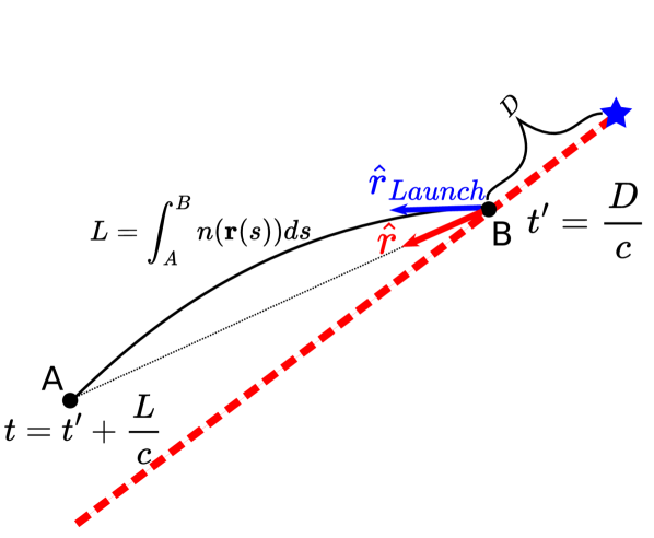
Figure 1: A diagram showing the line model of the cascade with important parameters highlighted. The first interaction point is marked by the blue star along with a receiver point A and an emission point B. The travel time is calculated from the optical distance of the ray. Also highlighted are the initial launch vector of the ray $\hat{r}_{Launch}$ and vector $\hat{r}$ pointing from emitter to receiver along a straight-line.

Due to the varying index of refraction, it is possible for a signal emitted in an emission time interval $\Delta t^{\prime}$ to arrive at the receiver in a shorter arrival time interval $\Delta t$. This boosting of the signal, purely due to geometry, can be described by the aforementioned geometric boostfactor: $\frac{\mathrm{d}t}{\mathrm{d}t^{\prime}}$. For a uniform index of refraction, one can prove that:

$$\frac{\mathrm{d}t}{\mathrm{d}t^{\prime}}=1-n\vec{\beta}^{*}\cdot\hat{r}$$ (3)

with $\vec{\beta}^{*}$ and $\hat{r}$ defined as in the end-point formalism. The link to boosting becomes clear when one considers the extreme case of maximum boosting $\frac{\mathrm{d}t}{\mathrm{d}t^{\prime}}=0$ as then Eq. 3 can be reduced to $\cos(\phi)=\frac{1}{n|\vec{\beta}^{*}|}$, with $\phi$ the angle between $\vec{\beta}^{*}$ and $\hat{r}$, allowing one to recover the standard expression for the Cerenkov angle.

III.1 Discussion of the Boostfactor

To investigate the correct way of formulating the boostfactor for non-uniform media, we compared different formulations of the boostfactor to $\frac{\mathrm{d}t}{\mathrm{d}t^{\prime}}$. A visualisation of this comparison for the line model of the cascade is given in Fig. 2, where the boostfactor was calculated as function of the difference between time of closest approach between shower front and receiver $t_{b}$ and emission time $t^{\prime}$. Results of the ray tracer are shown for a zenith angle of $65^{\circ}$ and a zenith angle of $85^{\circ}$ with receivers placed at a perpendicular distance of $1400$ m from the shower axis.

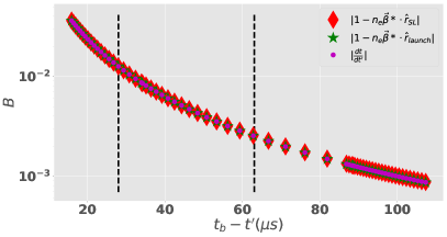
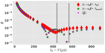
Figure 2: The boostfactor on a logarithmic scale as a function of the difference between time of closest approach and emission times for a zenith angle of $65^{\circ}$ (left) and $85^{\circ}$ (right). The dots (magenta) correspond to the numerically computed derivative, representing the true value of the boostfactor, while the diamonds (red) and stars (green) correspond to the boostfactor calculation with $\hat{r}$ and $\hat{r}_{\mathrm{Launch}}$ respectively. The area between the vertical black dashed lines denotes a typical region around the point where one would find the maximum amount of emitters ($X_{\mathrm{max}}$) to give an indication which part of the cascade causes the largest part of the emission.

From Fig. 2 one can see that the calculation of the boostfactor that uses the index of refraction at the emission point and the initial launch direction of the ray agrees with the numerically computed true boostfactor. This is a non trivial result which, while not analytically proven, has been verified for many different geometries and has already previously been applied to the simulation of radio emission from cascades passing from air into ice as seen for an in-ice receiver [20]. Fig. 2 also shows that the effects for low zenith angles remain minimal, but that the commonly used straight line calculation of the boostfactor can differ significantly from the correct result for very inclined showers. Care should be taken in interpreting these results, as relating the effects of a changing boostfactor to effects in expected received signal is highly non-trivial and is the subject of the following sections.

Note that the results shown in Fig. 2 represent only the denominator of Eq. 1. In order to have an idea of the full effect of moving to a curved ray path, one should also replace the $\hat{r}$ in the numerator of Eq. 1: $\hat{r}\times[\hat{r}\times\vec{\beta}^{*}]$. In order to estimate the effect of the numerator, consider a region close to an emitter where $n$ can be assumed to be constant. Assume also that $|\vec{\beta}^{*}|\approx 1$. Defining $\rho$ as the angle between $\hat{r}$ and $\vec{\beta}^{*}$ we can then write:

$$\frac{\hat{r}\times[\hat{r}\times\vec{\beta}^{*}]}{|1-n\vec{\beta}^{*}\cdot\hat{r}|}=\frac{\sin{\rho}}{|1-n\cos\rho|}.$$ (4)

A second point to consider is that in a realistic air shower geometry, there will be some spread regarding the direction of $\vec{\beta}^{*}$ around the shower axis. Fig. 3 illustrates how this spread can influence the radiation pattern of Eq. 4. Note that the values used for this plot are an exaggeration and that the typical spread of $\vec{\beta}^{*}$ would be of order $0.1^{\circ}$ around the shower axis [24].

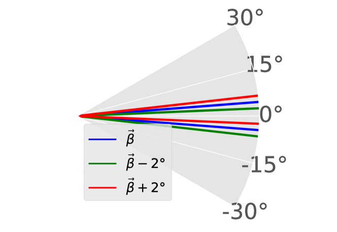
Figure 3: Polar plot showing the radiation pattern based on Eq. 4 with $n=1.003$. The blue line represents the radiation pattern at the Cerenkov angle for a horizontal $\vec{\beta^{*}}$ propagating along the line $0^{\circ}$. The red and green lines correspond to the radiation pattern where $\vec{\beta^{*}}$ is shifted up or down $2^{\circ}$. Note that this value is large to illustrate the effect of the spread in momentum around the shower axis. Realistic values are expected to be of the order $0.1^{\circ}$ [24]. A shift in initial direction could lead to a larger expected signal for some subset of emitters and a lower expected signal for some other subset, allowing the effects to potentially cancel out.

This spread in $\vec{\beta}^{*}$ could potentially cancel out the effects of a change in initial propagation direction due to ray curvature, as a shift in initial direction could lead to a larger expected signal for some subset of emitters and a lower expected signal for some other subset.

As part of this argument, related to the spread of momentum, one should also investigate the change in initial signal propagation direction induced by moving to a curved ray path. Fig. 4 shows the angle between initial signal travel direction and the shower axis for both a straight line path and a curved ray traced path for a geometry with a zenith angle of $85^{\circ}$, a similar geometry as used to obtain the results shown in Fig. 2. Also shown is the difference between the two angles, found to reach a maximum value of $0.05^{\circ}$.

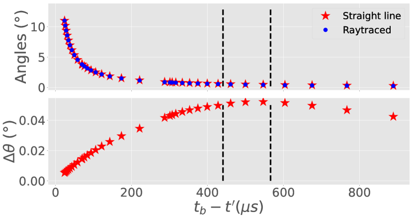
Figure 4: Top: The angle, in degrees, between the direction of initial propagation and the shower axis for both a ray traced path (blue dots) and a straight-line path (red stars) for a geometry with a zenith angle of $85^{\circ}$. Bottom: The difference between the straight line and ray trace angle , in degrees, shown in the top plot. Note that this difference reaches a relatively small value of $0.05^{\circ}$. The two black lines represent a typical region around $X_{\mathrm{max}}$ as in Fig. 2.

Note that while the effects shown in Fig. 2 show very large effects between ray traced and straight line trajectories on the boostfactor level, the small absolute difference in angles shown in Fig. 4 gives a more nuanced picture. As explained above: a spread in emitter momentum could potentially smear out the effect of moving to a curved ray path. We also mention that the difference between ray-trace and straight-line angles grew when moving to more inclined geometries. For the most inclined geometries these values could be of the order $0.1^{\circ}$, and hence, could be relevant for reconstruction purposes.

Finally, note that the $R$ present in Eq 1 is the geometrical distance between emitter and receiver. To verify that it should be the geometrical distance $R$ and not the optical path length $L$ one can look at the example shown in appendix D, where we calculate the electric field for a medium with constant $n>1$ and recover the standard coulomb field in the case of a stationary charge.

To investigate ray curvature effects on the simulated radio signal in a more complete manner, we use an adapted version of CoREAS which is able to modify the end-point calculation by use of tabulated data from the ray tracer. An explanation of this tabulation procedure is given in appendix A. Note that we assume all emitters to be on the shower axis for the calculation of the boostfactor, this is expected to be a reasonable assumption due to the distances between emitter and shower axis being small compared to the distances between emitter and receiver. A more in depth verification of this assumption is given in appendix B.

IV Simulation setup and geometry

We use a modified version of the CoREAS code included in the CORSIKA software where the calculation of the boostfactor is improved by use of raytracing data stored in tables. For this paper, we used version 7.7420 of the CORSIKA software.

For the simulation geometry we chose the configuration as shown in Fig. 5, where receivers were placed on a curved line of constant altitude following Earth’s curvature in a plane that fully contains the shower axis, defining the origin as the point where the shower axis crosses sea level. We then generate a shower with a specified zenith angle $\theta$ and a set azimuthal angle $\phi=0$. This layout of receivers includes the latest receiver positions for which the ray curvature is most pronounced and for which the effect of the changing boostfactor should be the largest.

Figure 5: Geometry used for CORSIKA/CoREAS simulations. Receivers are placed in the $\mathbf{Z},\mathbf{North}$ plane on a constant altitude. The coordinate origin is defined as in CORSIKA. Note that the receivers are placed on a constant altitude trajectory following the curvature of the earth.

The ray tracer is then used to generate a table for each receiver which allows the calculation of the correct launch vector $\hat{r}_{\mathrm{Launch}}$ from the straight-line vector $\hat{r}$ used during the calculation in standard CoREAS. A further explanation of the tabulation method and the mapping of $\hat{r}$ to $\hat{r}_{\mathrm{Launch}}$ is given in Appendix A. Through this tabulation, one can now compute the adapted $\hat{r_{\mathrm{Launch}}}$ without having to ray trace to each individual emitter during simulation.

For reference, the CoREAS simulations were set up with the following options:

• The high energy hadronic interaction model used was QGSJETII-04 and the low energy hadronic interaction model was URQMD1.3CR

• The primary chosen was always a proton with energy $10^{17}$.

• The thinning arguments were put to THIN: [$10^{-6}\ 10^{2}\ 0$]. The first value representing the fraction of the primary energy below which thinning is used. The second value gives a maximum weight until when thinning is used. The last value is used for radial thinning, which is turned off for a value of 0.

• The hadronic thinning was put to THINH: [$1\ 10^{2}$]. The values here are used to define a difference in thinning fraction and weights relative to electromagnetic thinning.

• The energy cuts applied through ECUTS for hadrons, muons, electrons and photons were put respectively at: [$0.3\ 0.3\ 4.01\cdot 10^{-4}\ 4.01\cdot 10^{-4}$] GeV.

• The time resolution for the CoREAS simulation was put at $20$ ns.

For the full discussion of these input parameters, we refer to the documentation available online [25].

V Effect of the boostfactor on received fluence

From the time traces obtained through CoREAS one can compute the received fluence $f$ at each receiver from a set of $N$ samples in time as [26]:

$$f=\epsilon_{0}c\Delta T\sum_{i=0}^{N-1}E^{2}(t_{i}),$$

with $\Delta T$ the width of each time bin. To now investigate the effect of the adapted boostfactor calculation we look at the effect on the received fluence. We do this by comparing the fluence $f_{RT}$ from a time trace where the calculation was done with the launch vector $\hat{r}_{\mathrm{Launch}}$ to the fluence $f$ from a time trace where the calculation was done with the connecting straight-line vector $\hat{r}$, as is done in standard CoREAS. This comparison is repeated for different values of the zenith angle $\theta$ and with pulses filtered to desired frequency ranges to get an understanding of what effect including a curved ray path has on the expected received fluence.

The fluence comparison for four different frequency ranges and five different zenith angles are given in Fig. 6, where we show the fluences calculated at different receivers as well as the ratio $\frac{f_{RT}}{f_{SL}}$ as a function of distance from the shower axis as measured from the projected positions of the observers in the shower plane. The fluence values here have been adapted to correct for early-late effects following the procedure as detailed in [27], with the important steps explained in appendix C. All showers were induced by a proton primary with energy $10^{17}$ eV and the magnetic field oriented fully in the $z$ direction with a strength of $50\ \mu$T.

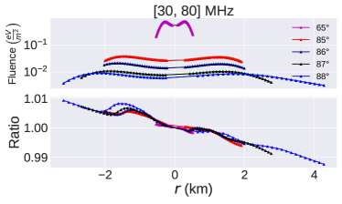
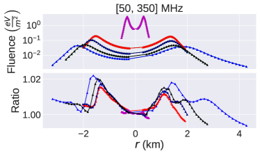
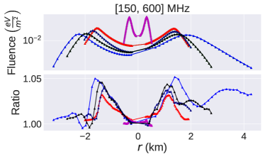
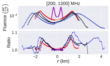
Figure 6: Simulated fluences for different frequency ranges for showers with zenith angles of $65^{\circ}$ (magenta), $85^{\circ}$ (red), $86^{\circ}$ ( navy blue), $87^{\circ}$ (black), $88^{\circ}$ (blue). Four frequency ranges are considered, where the top plot always shows the fluence as calculated from CoREAS traces. The lower plot shows the ratio $\frac{f_{RT}}{f}$ between the fluence calculated by using ray tracing data $f_{RT}$ and the fluence $f$ as calculated with an unaltered version of CoREAS. On the x-axis is the distance between the shower axis and the projected position of the observer in the shower plane, with negative values corresponding to early geometries and positive values to late geometries. The calculation of the projected distance to the shower axis is further explained in appendix C.

One can see that the relative error remains small for the less inclined shower of $65^{\circ}$, with a difference of order $0.1\%$. The difference becomes more apparent for the most inclined showers, but remains of the order of a few percent. We can conclude that the effect of improving the boostfactor calculation remains at the order of a few percent difference for frequencies up to $1.2$ GHz and zenith angles up to 88^∘.

An explanation for the relative difference between the fluences remaining small while the error on the boostfactor was simulated to be large can be found in the correct implementation of travel times in CoREAS. Due to this the coherence between different emitters is conserved, leading to a correct result for the bulk emission even though the amplitude for each individual emitter might have an associated error. This reasoning lies along the same line as the explanation found in [14, 15], namely that a straight-line path that takes into account the index of refraction profile only introduces a relatively small error of the order of $0.1$ ns in the signal travel time and that this small error does not introduce a significant effect at typically used radio frequencies. Aside from this timing based argument, the spread in momentum is also expected to cause a cancellation of effects.

Care should be taken when applying these results to macroscopic models, as there the contributions of different emitting elements are typically more significant. One should also note that no earth skimming effects were taken into account for this study, and that in general geometries where interaction between the radiation and ground become important were not considered here.

VI Summary and conclusion

In this paper we explained the concept of the geometric boostfactor and the implementation in CoREAS through the end-point formalism. We showed that the correct way of calculating the boostfactor is by use of the initial launch direction of the ray and the index of refraction value at the emitter. We implemented this adaption of the boostfactor calculation in CoREAS and evaluated the received fluence for a collection of receivers placed on a line. By comparing the results obtained with the ray tracing data to the results obtained with the standard implementation we found that the relative difference remained within a few percent in fluence. This while the difference for the different boostfactor calculations based on a line model of the cascade was found to be much larger. This apparent contradiction is explained firstly as due to the correct implementation of travel time in CoREAS as this lead to the correct coherence condition between different emitters and secondly due to the spread of particle momentum around the shower axis allowing a cancellation of the effects of moving to a curved ray path.

We conclude that for frequencies up to 350 MHz and zenith angles up to $88^{\circ}$ the effect of moving to a curved ray path remains negligible for most applications. Although the fluence pattern does not shift drastically, the 10 percent difference in fluence seen at GHz frequencies for $88^{\circ}$ could have non trivial effects on energy reconstruction. Higher frequency ($>1$ GHz) detection efforts tailored towards inclined geometries should therefore especially verify the effect of a few percent difference on energy reconstruction algorithms. Similarly, while the difference between the launch and straight line angle is seen to only reach values up to $0.1^{\circ}$ this could be significant when looking at sub-degree directional resolution. We thus also conclude that, while effects might seem relatively small, care must still be taken when assuming a straight line approximation for very inclined geometries when working at GHz frequencies. Especially when one seeks a high precision result in terms of directional or energy reconstruction.

VII Acknowledgments

This work has been supported by the the European Research Council under the EU-ropean Unions Horizon 2020 research and innovation programme. (grant agreement No 805486).
This work has been supported by the Flemish Foundation for Scientific Research. (FWO-G085820N).

Appendix A Tabulation of ray tracing data

The tables are generated using the ray tracer specified in the third section. For a specified zenith angle and receiver positions, rays are traced until they hit the shower axis. At the point B where a ray hits the shower axis the x components of both the launch vector and the unit vector along the straight-line between point B and the receiver are saved to a table. This is done for a dense sampling of the shower axis, allowing one to get a relation between the $x$-component of the straight-line vector $\hat{r}$ and the $x$-component of the launch vector $\hat{L}$. Note that due to the way these tables are constructed we implicitly assume that the emitter is placed at the shower axis. This is acceptable as we expect the distances between shower-axis and emitter to be small relative to the typical distances between emitter and receiver.

An explanation of how the tables are used is given below, with a diagram explaining the main steps given in Fig. 7.

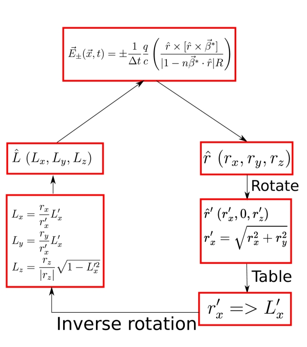
Figure 7: Diagram explaining the usage of tables during a CoREAS simulation, starting from the expression of the end-point formalism and ending with the construction of the launch vector $\hat{L}$ to replace the straight-line vector $\hat{r}.$

To explain how the tables are used first note that the ray tracer works with a 2D coordinate system, while CoREAS works with a 3D geometry. We therefore rely on spherical symmetry to reduce the 3D geometry in CoREAS to a 2D geometry where we can use the results from the ray tracer.

Our approach is as follows: assume an emitter and associated unit vector $\hat{r}=r_{x}\hat{x}+r_{y}\hat{y}+r_{z}\hat{z}$ pointing towards the receiver from the emitter along a straight-line. Due to spherical symmetry we can perform a rotation so that we can describe $\hat{r}$ using only the vertical and horizontal components:

$$\hat{r}=r_{x}^{\prime}\hat{x}^{\prime}+r_{z}\hat{z},$$

$$r_{x}^{\prime}=\sqrt{r_{x}^{2}+r_{y}^{2}}.$$

This $r_{x}^{\prime}$ of the straight-line vector is now used with the table to obtain the corresponding value $L^{\prime}_{x}$ of the launch vector from ray tracing. We then perform the inverse rotation back to the original frame, leading to:

$$L_{x}=\frac{r_{x}}{\sqrt{r_{x}^{2}+r_{y}^{2}}}L_{x}^{\prime},$$

$$L_{y}=\frac{r_{y}}{\sqrt{r_{x}^{2}+r_{y}^{2}}}L_{x}^{\prime},$$

$$L_{z}=\frac{r_{z}}{|r_{z}|}\sqrt{1-L_{x}^{{}^{\prime}2}},$$

where we obtained $L_{z}$ from $L^{\prime}_{x}$ and the fact that the vector must have norm 1. Note that we also defined the sign of $L_{z}$ to be equal to the sign of the $z$ component of the original straight-line vector $\hat{R}$. In practice this means that we restrict ourselves to direct rays.

Appendix B Verification of line model

For the results in this paper, the launch vector was calculated from tabulated data for which a simple line model of the cascade was used. This means that changes in the launch vector due to lateral displacement from the shower axis are not taken into account. This approach is expected to be valid due to the relatively small distances for emitters from the shower axis with respect to the distance between emitter and receiver.

A verification of this assumption was made for a geometry of zenith angle $85^{\circ}$, where we traced rays to a region around a typical value of $X_{\mathrm{max}}$. We then compared the horizontal components of:

• The straight-line unit vector connecting emitter and receiver,

• The initial launch unit vector of the ray connecting emitter and receiver obtained through direct ray tracing,

• The reconstruction of the launch unit vector using tabulation.

The result of this comparison can be found visualised in Fig. 8.

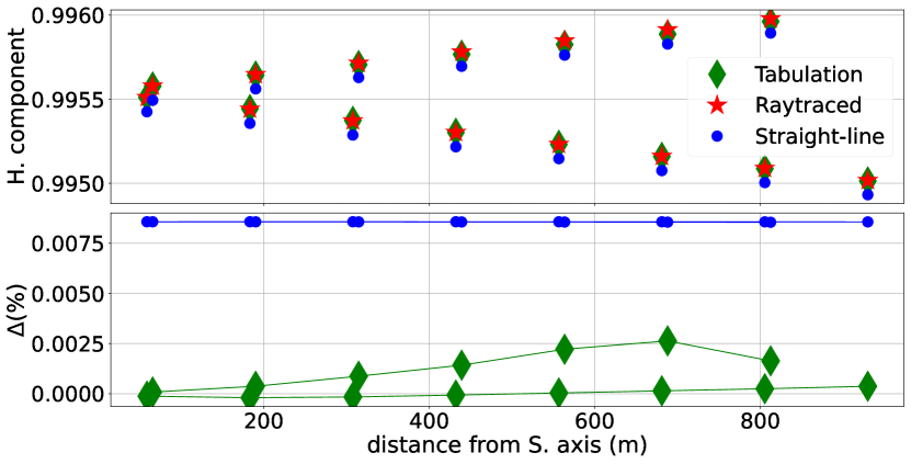
Figure 8: A verification of the line model. Shown in the top plot are the horizontal component of unit vectors used in the boostfactor calculation. Red is the (correct) value for the launch vector, blue is the value for the straight-line vector and green is the value reconstructed from our tabulation procedure. The bottom plot shows the difference between these components as a percentage of the launch vector value.

This result is interesting because, while the value of the launch vector component can vary a relatively larger amount within a few 100 m of the shower axis, the difference with the straight-line component stays near constant. This allows for a good reconstruction from tabulation.

Appendix C Accounting for early-late effects

The accounting of early-late effects in this work follows closely the procedure explained in [27]. A short summary is given in this appendix.

Early late effects arise from a difference in distance depending on receiver position. In the context of radiation coming from inclined air shower geometries the associated difference in travel time can be interpreted as a difference in geometrical distance between $X_{\mathrm{max}}$ and the receiver as shown in Fig. 9. A receiver position with a lower associated travel time is often called ’early’, while those with a higher associated travel time are called ’late’ receivers.

To quantize and correct early late effects: consider radiation coming from the shower maximum in the form of spherical waves. The amplitude of the electric field then scales as $\frac{1}{r}$. The goal is now to scale the amplitude seen by a receiver to match the amplitude that would be seen by the associated projection in the shower plane.

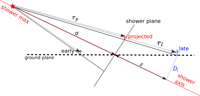
Figure 9: A diagram showing the shower axis of an inclined shower alongside an early and late receiver. also indicated are some distances used in the derivation of the correction factor used to account for early late effects as well as the projection on the shower plane of the late receiver position

Consider now the electric field amplitude $E_{l}$ as seen by the late receiver shown in 9. The relation to the electric field amplitude $E_{p}$ as seen by the projected receiver in the shower axis is then:

$$E_{p}=\frac{r_{l}}{r_{p}}E_{l}.$$

Since $\frac{r_{l}}{r_{p}}=\frac{d+z}{d}$ this can be rewritten as:

$$E_{p}=F\cdot E_{l},$$

$$F=\frac{d+z}{d}.$$

Note that z is positive for late receivers and negative for early receivers.

Since fluence scales with the square of the electric field amplitude the correction factor between $f_{l}$ seen by the late receiver to the associated fluence seen from the projected receiver position $f_{p}$ is

$$f_{p}=F^{2}\cdot f_{l}$$

The derivation of the correction factor for early receivers is identical, the only difference being that $z$ is negative and thus $c<1$.

The correction factor c can also be used to find the distance of the projected receiver position from the shower axis:

$$\frac{D_{l}}{D_{p}}=\frac{d+z}{d}=F$$

It is this $D_{p}$ which is shown on the horizontal axes of the figures in Fig. 6.

Appendix D Geometrical path length and Optical path length

To verify that the electric field amplitude should scale with the inverse of the geometrical distance $R$ and not the optical distance $L$, one can calculate the electric field of a moving charge for a medium with constant index of refraction $n>1$:

$$\mathbf{E}=-\frac{1}{4\pi\epsilon_{0}}\frac{qc}{(Rc-n\mathbf{R}\cdot\mathbf{v})^{3}}\Bigg{[}\left(n\mathbf{v}-\frac{\mathbf{v}}{n}+\frac{R}{c}\mathbf{a}\right)\cdot(Rc-n\mathbf{R}\cdot\mathbf{v})\\ +\left(\frac{nR}{c}\cdot\mathbf{v}-n^{2}\mathbf{R}\right)\left(\frac{c^{2}}{n^{2}}-v^{2}+\mathbf{R}\cdot\mathbf{a}\right)\Bigg{]},$$

where bold symbols represent vectors. $\mathbf{v}$ is the velocity, $\mathbf{a}$ represents the acceleration, $v=|\mathbf{v}|$ and $R=|\mathbf{R}|$. The derivation of this result closely follows the steps detailed in [28].

If we now consider the simplest case of a stationary charge $q$, for which both velocity and acceleration terms vanish, we arrive at the following expression for the electric field:

$$\mathbf{E}=\frac{1}{4\pi\epsilon_{0}}\frac{q}{c^{2}}\frac{1}{R^{3}}\cdot n^{2}\mathbf{R}\cdot\frac{c^{2}}{n^{2}},$$

$$\mathbf{E}=\frac{1}{4\pi\epsilon_{0}}\frac{q}{R^{3}}\cdot\mathbf{R}.$$

This is the standard coulomb field, which we find scales with the inverse square of the geometrical distance $\frac{1}{R^{2}}$. From this result we conclude that the $R$ in Eq. 1 should represent the geometrical distance $R$ and not the optical path length $L$.

References

- Abreu et al. [2021] P. Abreu et al. (Pierre Auger), The energy spectrum of cosmic rays beyond the turn-down around eV as measured with the surface detector of the Pierre Auger Observatory, Eur. Phys. J. C 81, 966 (2021), arXiv:2109.13400 [astro-ph.HE] .
- Abu-Zayyad et al. [2012] T. Abu-Zayyad et al. (Telescope Array), The Energy Spectrum of Telescope Array’s Middle Drum Detector and the Direct Comparison to the High Resolution Fly’s Eye Experiment, Astropart. Phys. 39-40, 109 (2012), arXiv:1202.5141 [astro-ph.IM] .
- Abbasi et al. [2021] R. Abbasi et al. (IceCube), The IceCube high-energy starting event sample: Description and flux characterization with 7.5 years of data, Phys. Rev. D 104, 022002 (2021), arXiv:2011.03545 [astro-ph.HE] .
- Barrella et al. [2011] T. Barrella, S. Barwick, and D. Saltzberg, Ross Ice Shelf in situ radio-frequency ice attenuation, J. Glaciol. 57, 61 (2011), arXiv:1011.0477 [astro-ph.IM] .
- Barwick et al. [2005] S. Barwick, D. Besson, P. Gorham, and D. Saltzberg, South Polar in situ radio-frequency ice attenuation, J. Glaciol. 51, 231 (2005).
- Besson et al. [2008] D. Z. Besson et al., In situ radioglaciological measurements near Taylor Dome, Antarctica and implications for UHE neutrino astronomy, Astropart. Phys. 29, 130 (2008), arXiv:astro-ph/0703413 .
- Avva et al. [2015] J. Avva, J. M. Kovac, C. Miki, D. Saltzberg, and A. G. Vieregg, An in situ measurement of the radio-frequency attenuation in ice at Summit Station, Greenland, J. Glaciol. 61, 1005 (2015), arXiv:1409.5413 [astro-ph.IM] .
- Huege [2016] T. Huege, Radio detection of cosmic ray air showers in the digital era, Phys. Rept. 620, 1 (2016), arXiv:1601.07426 [astro-ph.IM] .
- Huege [2023] T. Huege (Pierre Auger), The Radio Detector of the Pierre Auger Observatory – status and expected performance, EPJ Web Conf. 283, 06002 (2023), arXiv:2305.10104 [astro-ph.IM] .
- Álvarez-Muñiz et al. [2020] J. Álvarez-Muñiz et al. (GRAND), The Giant Radio Array for Neutrino Detection (GRAND): Science and Design, Sci. China Phys. Mech. Astron. 63, 219501 (2020), arXiv:1810.09994 [astro-ph.HE] .
- Southall et al. [2023] D. Southall et al., Design and initial performance of the prototype for the BEACON instrument for detection of ultrahigh energy particles, Nucl. Instrum. Meth. A 1048, 167889 (2023), arXiv:2206.09660 [astro-ph.IM] .
- Huege et al. [2013] T. Huege, M. Ludwig, and C. W. James, Simulating radio emission from air showers with CoREAS, AIP Conf. Proc. 1535, 128 (2013), arXiv:1301.2132 [astro-ph.HE] .
- Alvarez-Muniz et al. [2012] J. Alvarez-Muniz, W. R. Carvalho, Jr., M. Tueros, and E. Zas, Coherent Cherenkov radio pulses from hadronic showers up to EeV energies, Astropart. Phys. 35, 287 (2012), arXiv:1005.0552 [astro-ph.HE] .
- Alvarez-Muñiz et al. [2015] J. Alvarez-Muñiz, W. R. Carvalho, D. García-Fernández, H. Schoorlemmer, and E. Zas, Simulations of reflected radio signals from cosmic ray induced air showers, Astropart. Phys. 66, 31 (2015), arXiv:1502.02117 [astro-ph.HE] .
- Schlüter et al. [2020] F. Schlüter, M. Gottowik, T. Huege, and J. Rautenberg, Refractive displacement of the radio-emission footprint of inclined air showers simulated with CoREAS, Eur. Phys. J. C 80, 643 (2020), arXiv:2005.06775 [astro-ph.IM] .
- Werner and Scholten [2008] K. Werner and O. Scholten, Macroscopic Treatment of Radio Emission from Cosmic Ray Air Showers based on Shower Simulations, Astropart. Phys. 29, 393 (2008), arXiv:0712.2517 [astro-ph] .
- Deaconu et al. [2018] C. Deaconu, A. G. Vieregg, S. A. Wissel, J. Bowen, S. Chipman, A. Gupta, C. Miki, R. J. Nichol, and D. Saltzberg, Measurements and Modeling of Near-Surface Radio Propagation in Glacial Ice and Implications for Neutrino Experiments, Phys. Rev. D 98, 043010 (2018), arXiv:1805.12576 [astro-ph.IM] .
- Prohira et al. [2021] S. Prohira et al. (Radar Echo Telescope), Modeling in-ice radio propagation with parabolic equation methods, Phys. Rev. D 103, 103007 (2021), arXiv:2011.05997 [astro-ph.IM] .
- Windischhofer et al. [2023] P. Windischhofer, C. Welling, and C. Deaconu, Eisvogel: Exact and efficient calculations of radio emissions from in-ice neutrino showers, PoS ICRC2023, 1157 (2023).
- De Kockere et al. [2024] S. De Kockere, D. Van den Broeck, U. A. Latif, K. D. de Vries, N. van Eijndhoven, T. Huege, and S. Buitink, Simulation of radio signals from cosmic-ray cascades in air and ice as observed by in-ice Askaryan radio detectors, Phys. Rev. D 110, 023010 (2024), arXiv:2403.15358 [astro-ph.HE] .
- James et al. [2011] C. W. James, H. Falcke, T. Huege, and M. Ludwig, General description of electromagnetic radiation processes based on instantaneous charge acceleration in “endpoints”, Phys. Rev. E 84, 056602 (2011).
- Ludwig and Huege [2011] M. Ludwig and T. Huege, REAS3: Monte Carlo simulations of radio emission from cosmic ray air showers using an ’end-point’ formalism, Astropart. Phys. 34, 438 (2011), arXiv:1010.5343 [astro-ph.HE] .
- Holm [2011] D. Holm, Geometric Mechanics - Part I: Dynamics And Symmetry (2nd Edition) (World Scientific Publishing Company, 2011).
- Lafebre et al. [2009] S. Lafebre, R. Engel, H. Falcke, J. Horandel, T. Huege, J. Kuijpers, and R. Ulrich, Universality of electron-positron distributions in extensive air showers, Astropart. Phys. 31, 243 (2009), arXiv:0902.0548 [astro-ph.HE] .
- D. Heck and Pierog [2024] T. H. D. Heck and T. Pierog, Corsika documentation (2024), available at: https://www.iap.kit.edu/corsika/70.php.
- Aab et al. [2016] A. Aab et al. (Pierre Auger), Energy Estimation of Cosmic Rays with the Engineering Radio Array of the Pierre Auger Observatory, Phys. Rev. D 93, 122005 (2016), arXiv:1508.04267 [astro-ph.HE] .
- Schlüter and Huege [2023] F. Schlüter and T. Huege, Signal model and event reconstruction for the radio detection of inclined air showers, JCAP 01, 008, arXiv:2203.04364 [astro-ph.HE] .
- Griffiths [2017] D. J. Griffiths, Introduction to Electrodynamics, 4th ed. (Cambridge University Press, 2017).