Shortcuts to adiabaticity in open quantum critical systems
Shishira Mahunta
Department of Physical Sciences, IISER Berhampur, Berhampur 760010, India
Victor Mukherjee
Department of Physical Sciences, IISER Berhampur, Berhampur 760010, India
Abstract
We study shortcuts to adiabaticity (STA) through counterdiabatic driving in quantum critical systems, in the presence of dissipation. We evaluate unitary as well as non-unitary controls, such that the system density matrix follows a prescribed trajectory corresponding to the eigenstates of a time-dependent reference Hamiltonian, at any instant of time.
The strength of the dissipator control term for the low energy states show universal scaling close to criticality. Using the example of the transverse-field Ising model, we show that in contrast to STA in closed quantum critical systems, here STA may require multi-body interactions terms, even away from criticality, owing to change in entropy of the time-dependent target state. Further, the associated heat current shows extremum, while power dissipated changes curvature, close to criticality, and analogous to unitary control, no operational cost is associated with implementation of the exact counterdiabatic Hamiltonian. We expect the counterdiabatic protocol studied here can be of fundamental importance for understanding STA in many-body open quantum systems, and can be highly relevant for varied topics involving open many-body quantum systems, such as quantum computation and many-body quantum heat engines.
Quantum systems driven out of equilibrium in general show non-adiabatic excitations. Consequently, shortcuts to adiabaticity (STA) has been developed in the recent years, which provides an alternative pathway to effective adiabatic evolution, even for finite rates of driving [1]. STA can aid in quantum computation [2], can be utilized for the preparation of given target states in finite times [3, 4], and also has been shown to be highly beneficial for enhancing the output of quantum thermal machines [5, 6].
STAs can be engineered in both classical [7, 8] and quantum systems [9] and by now have been demonstrated in a wide variety of experiments [9, 10, 11].
A universal approach to implementing STA in closed quantum systems relies on counterdiabatic driving (CD) [12, 13, 14], also known as transitionless quantum driving [15]. This approach is based on application of a control Hamiltonian , such that the total Hamiltonian ensures effective adiabatic dynamics corresponding to a reference Hamiltonian , which is modulated in time at a finite rate.
In general, Kibble-Zurek mechanism dictates the generation of non-adiabatic excitations in many-body quantum systems driven through quantum phase transitions [16, 17]. However, as shown in Ref. [18], implementation of STA protocol can be particularly challenging in quantum critical systems (QCSs), owing to the presence of highly non-local control terms involving multi-spin interactions close to criticality. In addition, engineering STA through counterdiabatic driving may require detailed knowledge about the eigen spectrum of the quantum system, which can be highly non-trivial in many-body quantum systems.
These requirements can be prohibitive in many applications, such as in quantum annealing [19] and quantum computing [2].
Much of the ensuing work on STA in quantum critical systems has focused on alleviating these challenges [20, 21, 22, 23, 24, 25, 26], with an eye on applications on quantum computation and optimization [27, 2, 28, 29]. In the recent years approximate counterdiabatic protocols have been developed, which removes the requirement of a detailed knowledge about the eigenspectrum of a system, and hence can be highly beneficial for implementation of STA in many-body quantum systems [30, 31, 32].
The combination of digital quantum simulation of the CD control in combination with variational ansatz has led to a new class of quantum algorithms, known as digital counterdiabatic quantum algorithms [33, 34, 35, 36, 37].
The works mentioned above focused on STA in close quantum systems involving unitary dynamics. However, developing STA in the presence of dissipation can be crucial as well, for their application potential in open quantum systems, such as for fast cooling or heating of quantum systems [38, 39], or for enhancing the output of quantum heat engines [40].
The development of STA in quantum open systems is in its infancy and only a few results are known to date [41, 42, 38, 43, 44, 45, 46]. A notable experiment in this context has been reported in open circuit quantum electrodynamics [47]. A universal framework generalizing CD, applicable both to isolated and open quantum systems, was put forward in [38].
This scheme
finds applications on thermodynamics of quantum systems [48].
This formulation demands evolution of the system density matrix along a prescribed trajectory, for example, the instantaneous thermal state of a time-dependent reference Hamiltonian .
The dynamics is non-unitary, and consequently implementation of the control protocol requires CD dissipator terms that govern the change of the eigenvalues, in addition to a CD Hamiltonian. This formalism avoids the notion of adiabaticity in open systems in terms of Jordan blocks, inherent to other approaches [49, 41, 46].
The application of the counterdiabatic scheme in open quantum systems to date has been restricted to single-particle quantum systems. In view of the challenges of applying STA in closed QCS, one can anticipate non-trivial features associated with application of STA in
finite time open QCSs as well. Chartering these difficulties is the focus of this work and we utilize the paradigmatic transverse field quantum Ising model as a testbed. This is both of fundamental relevance to understanding how STAs generalize to many-body open quantum systems and for applications such as quantum annealing [19, 50, 51], quantum metrology [52, 53, 54, 55], and the engineering of quantum thermodynamic devices [56, 57, 58], involving open QCSs. Notably, our analysis shows that in stark contrast to closed QCSs, STA in the presence of dissipation may involve many-body control terms even away from criticality.
We present the STA protocol in general open quantum systems driven out of equilibrium in Sec. I. We then focus on the transverse Ising model in the presence of a Fermionic bath Sec. II; we focus on the low temperature regime in Sec. II.1, followed by real space description of the CD control terms in Sec. II.2. We then study power and heat current associated with the STA control in Sec. III. Finally, we conclude in Sec. IV.
I General setup
We consider the time-evolution of a generic many-body system encoded in the trajectory of the density matrix as a function of time. Its spectral decomposition can be recast in the form of an instantaneous Gibbs state at all times, with respect to a time-dependent Hamiltonian , i.e.,
(1)
Here, is the energy of the -th instantaenous energy eigenstate with respect to at time , with for ; .
Following Ref. [38], we note that
the equation of motion of involves a generator that is not unitary, and requires both unitary and non-unitary control terms. Specifically, the trajectory obeys the master equation
(2)
Here, , and
(3)
is the counter diabetic Hamiltonian with respect to [59, 60], while
(4)
where is the rank of .
One can evaluate the coefficient corresponding to a transition from the -th energy state to the -th energy state () as (see Appendix A for details)
(5)
As expected, the low-temperature limit ( ) is associated with high rates of transitions to the lower energy states, as signified by for (see Eq. (5)).
For the lower energy states in the low temperature limit we get
(6)
where we have considered for .
Further, we have close to criticality, where ) denotes the distance from the quantum critical point; here () is the corresponding correlation length (time) exponent, while denotes the size of the system [61]. Consequently in this regime one has
(7)
signifying a diverging close to criticality for , while results in . We note that the vanishing close to criticality for is in stark contrast to unitary dynamics, where in general the strength of the counter-diabatic Hamiltonian diverges close to criticality. This can be related to the fact that for unitary dynamics, the counter-diabatic Hamiltonian is associated with a sudden change of the ground state of the Hamiltonian close to criticality. In contrast, here is related to , which can be small for and .
II STA in a free-Fermionic system: transverse Ising model
We now focus on the specific example of a free-Fermionic system coupled to a Fermionic bath [62].
We consider the transverse Ising model,
(8)
which exhibits a quantum phase transition between a paramagnetic phase and a ferromagnetic phase () at the critical points [61].
One can make use of the Jordan-Wigner transformation followed by a Fourier transformation to arrive at the free-Fermionic form
(9)
in the basis ,
where we have assumed [63]. We assume the th mode starts in its instantaneous thermal equilibrium (Gibbs) state at . However, as the transverse field is changed, one can expect the system to go out of thermal equilibrium for finite rates of . Consequently, here we evaluate the Lindblad control protocol which ensures that the system remains in its instantaneous local Gibbs state , given by
(10)
in the energy eigenbasis for the k-th mode, at all times. In this expression,
and . The energy gap vanishes at the critical point for [63, 64]. Furthermore, free-Fermionic nature of the system implies , thus allowing us to treat each mode independently.
where denotes any of the four instantaneous eigenstates for the -th mode, given by
(12)
Here, is the ground state, and are degenerate second and third excited states, and is the highest excited state. The explicit forms of the Lindblad operators and the corresponding coupling rates are derived given in Appendix B.
We note that denotes the rate of transition from the state to the state , for the mode .
II.1 Low temperature regime
In this section we consider the low-temperature limit of . In this regime the instantaneous Gibbs state is close to the instantaneous ground state for all times. Consequently all the ’s denoting excitation to higher energy states are exponentially small (, see Eq. (35)), while the non-zero rates signifying transitions to the lower or degenerate energy states are given by
(13)
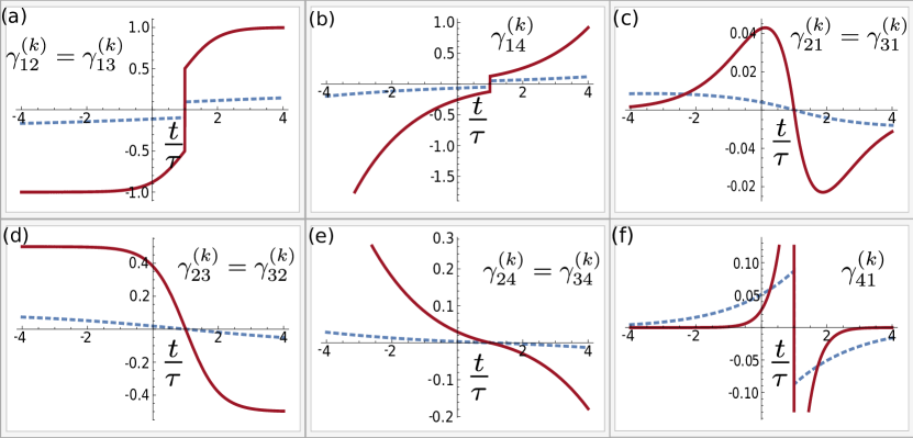
Figure 1: Plot showing the variation of with time for (See Eq. 35) . The red solid line refers to the low temperature regime, and the blue dashed line refer to the high temperature regime, . As shown here, ’s change sign and may show non-analytic behavior close to the quantum critical point at .
We show the variations of ’s with time for the critical mode in Fig. 1. As shown in Fig. 1, the ’s change sign, and may show show non-analytic behavior at . The time dependence of the ’s follow from the temporal variation of the energy eigenvalues (see Appendix C). A positive (negative) signifies transfer of population from the -th (-th) energy state to the -th (-th) energy state; this in turn results in the ’s changing sign at (see Eq. (13)), thus ensuring that the th mode stays in it’s instantaneous Gibbs state at all times. Further, diverges for large , implying high rates of population transfer from the highest excited state to other states for large , as expected.
II.2 STA in real space
As discussed above, the Lindblad operators are relatively simple in the momentum space, where they involve only modes (see Eqs. (11) and (12)). In order to arrive at the spin space representation of the control terms, without loss of generality we focus on , which appears in the master equation Eq. (2) for a single mode, as a representative term. This will include terms of the form
(14)
where
(15)
One can show that in the spin space, this will result in multi-body interaction terms of the form (see Appendix D for details)
(16)
where we have taken into account , and assumed such that . Here and . Further, in the limit of large Eq. (16) reduces to
(17)
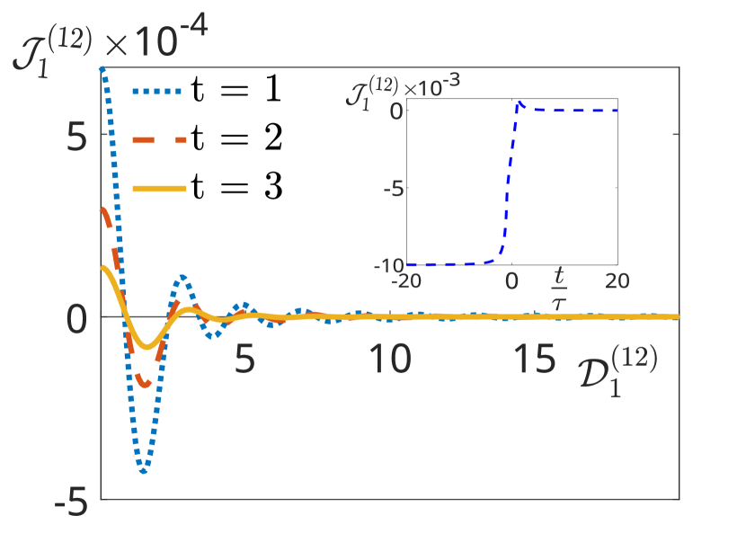
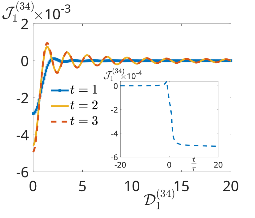
The terms on the r.h.s. of Eq. (17) can be expected to vanish in the limit of large . This is also verified by Fig. 2, where it is shown that decreases rapidly with , implying one can restrict to small values only. However, we get particle interactions in for a finite , where . Moreover, these multi-particle interactions persist even far away from criticality, as well as for , as signified by non-zero values of for in Fig. 2, or non-zero values of , corresponding to the term(see Appendix D), for in Fig. 5. This can be a signature of the fact that in contrast to unitary evolution, STA in open quantum systems requires control of entropy even away from criticality, which in turn necessitates multi-particle interactions in the control terms.
Figure 2: The main plot shows variation of as a function of and the inset shows variation of as a function of when . Here , , (see Eqs. (16) and (50)).
III Power and heat current under STA protocol
In this section, we focus on the costs of the STA protocol, as determined by the corresponding heat current and power .
III.1 Heat current
The total heat current for a generic system in the presence of STA is given by [65]
(18)
The cyclic property of trace implies , thus ensuring that can be written as a sum of bare and counterdiabatic parts (see Appendix E):
Where we have used [38].
On the other hand, for the counterdiabatic term we have (see Eq. (3)):
(21)
thus showing that the is not associated with any heat current.(see Eq. (54) for a detailed derivation)
In the case of the transverse Ising model considered here, one has , where (see Sec. II and Eq. (20)),
(22)
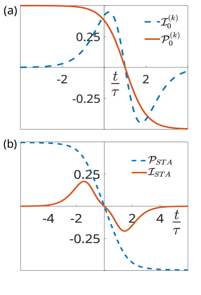
As shown in Eq. (22) and Fig. 3(a), is positive when the energy levels approach each other for , signifying heat flow to the system. In contrast, the heat flow direction is reversed () for , when the energy gaps diverge from each other. Consequently, the total heat current is positive (negative) for (), shows extremum values close to criticality , and approaches zero for , when the steady state does not change appreciably with time (see Fig. 3 (b)).
Figure 3: (a) Variation of heat current (Cf. Eq. (22)) and power (Cf. Eq, (26)) with time for the transverse Ising model, for . (b) Variation of total current and total power with time for the transverse Ising model in the thermodynamic limit. Here .
III.2 Power
We now focus on the power associated with the control. As before, we
express the total power by a sum of two components [65]:
(23)
One can evaluate as follows:
(24)
The normalisation condition implies . Therefore, for a generic system reads
(25)
On the other hand, as we discuss in detail in Appendix E, it can be shown that . This is reminiscent of unitary dynamics, where it has been shown that work associated with exact counterdiabatic Hamiltonian is zero [66].
In case of the transverse Ising model we have , where
(26)
As shown in Fig. 3(b), saturates to constant values far away from criticality, owing to the fact that the steady state does not change appreciably with time for (see Eqs. (10) and (12)).
As discussed above, the heat current as well as the power vanish, signifying the absence of any operational cost associated with the counterdiabatic Hamiltonian . However, we note that the heat current and power dissipated are still non-zero for the bare Hamiltonian (see Fig. 3(b)). Furthermore, additional implementational costs may arise in a specific experimental setups used for realizing the STA protocol [66].
IV Conclusions
We have studied shortcuts to adiabaticity in quantum critical systems driven out of equilibrium in the presence of a dissipative environment. We have derived non-Markovian Lindblad operator control terms required to ensure that the system always stays in its instantaneous thermal equilibrium state. The strengths of the Lindblad operator exhibits universal scaling close to a quantum phase transition for the low energy states. Furthermore, in stark contrast to STA in unitary dynamics, where control becomes most relevant close to criticality, here control is essential even away from a phase transition, as signified by non-zero values of for large energy gaps (see Eq. (5)). This can be attributed to change in entropy of the instantaneous thermal equilibrium state (Cf. Eq. (1)) even away from criticality for a time-dependent Hamiltonian.
We have then focused on the specific example of a transverse Ising spin chain coupled to a dissipative Fermionic bath. We have considered control such that each momentum mode of the system always remains in its instantaneous Gibbs state Eq. (10). The control Lindblad operators assume a simple form in the momentum representation (Cf. Eqs. (11) and (12)) that may be amenable to an experimental realization. However, these operators involve multi-body interaction terms in the spin space representation, even away from criticality (see Eq. (16)). We have also studied the heat current and power associated with the non-unitary dynamics. Interestingly, , signifying application of counterdiabatic Hamiltonian does not incur any operational cost. In contrast the vanishing of the energy gap close to criticality is reflected by assuming maximum close to . On the other hand, the heat current approaches zero for , when the steady state fails to change appreciably with time (see Fig. 3). The associated power saturates to constant value for away from criticality() when the energy eigenvalues changes with time at a constant rate .
Finally, we note that the control protocol presented here can be expected to be highly relevant for development of various quantum technologies, such as finite-time quantum heat engines involving isothermal strokes [67]; application of STA can be expected to significantly enhance the output of such heat engines [5, 6, 58]. Furthermore, several currently existing platforms, for example, quantum simulators [68, 69, 70] based on trapped ions [71] and Rydberg atoms [72, 73] may be ideal for experimental realization of the STA method discussed above.
Acknowledgements.
V.M. acknowledges Adolfo del Campo for helpful discussions during various stages of the work. V.M. also acknowledges support from the University of Luxembourg, where part of the work was done, support from Science and Engineering Research Board (SERB) through MATRICS (Project No.
MTR/2021/000055) and a Seed Grant from IISER Berhampur.
Appendix A General scalings in the limit
For transitions from an energy level to an energy level , we have
(27)
Again, . As a result,
(28)
For the lower energy states in the low temperature limit we get
(29)
where we have considered for .
Appendix B Lindblad operators and dissipation rates
The operators are as follows:
(30)
We have
(31)
where is the identity operator corresponding to the th mode.
Similarly,
(32)
It follows that
(33)
Proceeding as above, one can show that the different Lindblad operators introduced in Eqs. (11) and (12) are given by:
(34)
The s for the mode are given by
(35)
Appendix C Equation of motion:
The dynamical equation of motion of the system following the instantaneous thermal state (See Eq. (1) and Fig. 4) can be written as [38]
(36)
(37)
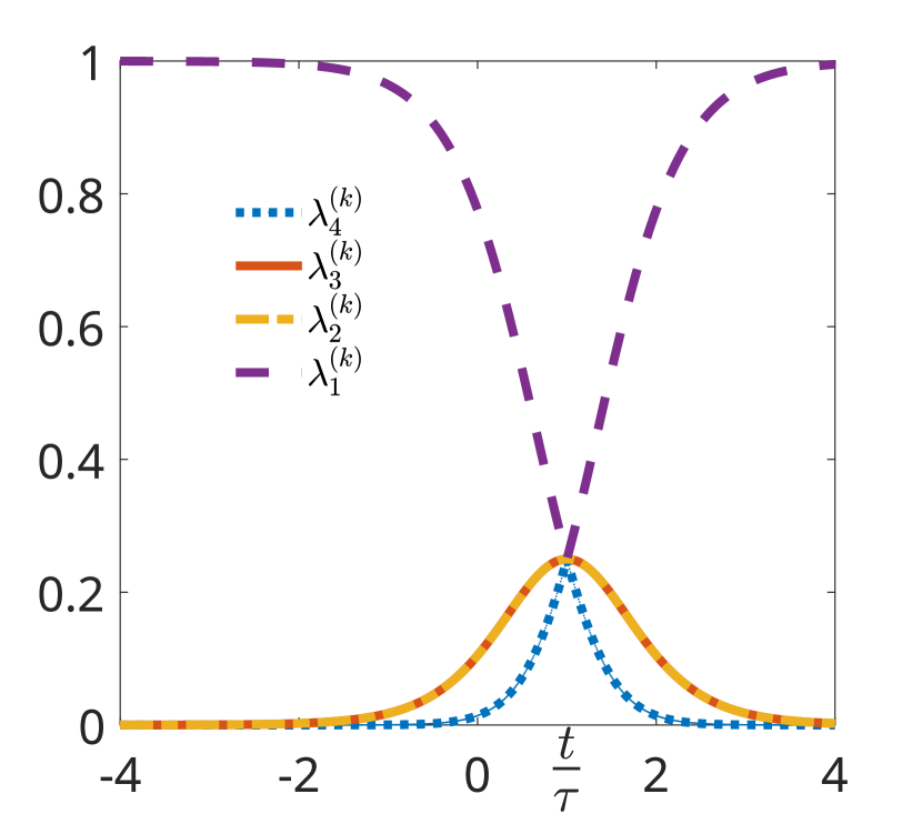
Figure 4: Thermal population of the ground state, and of the degenerate second and third excited states, and of highest excited state, with . Here , . The energy level populations becomes equal at the quantum critical point .
where we have used the relation . Comparing Eqs. (36) and (37) we get
Appendix D Control terms in the real space
We focus on a particular term involved in the master equation: . This will lead to terms of the form
The operators follow the anti-commutation relations
(42)
Consequently,
(43)
Assume such that . One then finds
(44)
where and , and we have used .
Furthermore, one can rewrite as
(45)
Term 2: Similarly, the other non-zero term will be of the form
(46)
Here
(47)
and we have assumed . The remaining two terms will involve and , and therefore will vanish, owing to the commutation relations satisfied by the Fermionic operators and .
Redefining the variables , we get
(48)
terms:
We note that in case of , the most significant contributions arise from and , which are responsible for deexcitation of the system to its instantaneous ground state (see Eq. (13)).
Proceeding as above, one can show that will contain terms of the form
Here , and in the limit of large , we have
(50)
Figure 5: Variation of (a) as a function of and (b) as a function of when . Here , , ; see Eqs. (16) and (50).
As shown in Figs. 2 and 5, both and decrease rapidly with and , respectively, implying one can restrict and to small values only. However, we note that even for , we will have multi-body interaction terms in the control Lindblad operators.
We note that by making the transformations in Eq. (D) we get
(51)
Appendix E Heat currents and Power
Heat Current: We have
(52)
Here by construction, while owing to cyclic property of trace. Further,
Power: We evaluate the power dissipated due to the counterdiabetic Hamiltonian in presence of a non-unitary evolution by considering the desired path for the system to be the instantaneous thermal state (Cf. Eq.(1)).
One can use the completeness relation, to get
(55)
Further, the normalisation condition leads to
(56)
Now we use Eq.(55) and Eq.(56) to evaluate the time derivative of the (C.f Eq.(3)),
(57)
Finally, we can use Eq.(57) to evaluate as follows,
(58)
References
Chen et al. [2010]X. Chen, A. Ruschhaupt, S. Schmidt, A. del Campo, D. Guéry-Odelin, and J. G. Muga, Fast optimal frictionless atom cooling in harmonic traps: Shortcut to adiabaticity, Phys. Rev. Lett. 104, 063002 (2010).
Santos and Sarandy [2015]A. C. Santos and M. S. Sarandy, Superadiabatic controlled evolutions and universal quantum computation, Scientific Reports 5, 15775 (2015).
Yao et al. [2021]J. Yao, L. Lin, and M. Bukov, Reinforcement learning for many-body ground-state preparation inspired by counterdiiabatic driving, Phys. Rev. X 11, 031070 (2021).
Kolodrubetz et al. [2017]M. Kolodrubetz, D. Sels, P. Mehta, and A. Polkovnikov, Geometry and non-adiabatic response in quantum and classical systems, Physics Reports 697, 1 (2017), geometry and non-adiabatic response in quantum and classical systems.
Campo et al. [2014]A. d. Campo, J. Goold, and M. Paternostro, More bang for your buck: Super-adiabatic quantum engines, Sci. Rep. 4, 6208 (2014).
Hartmann et al. [2020a]A. Hartmann, V. Mukherjee, W. Niedenzu, and W. Lechner, Many-body quantum heat engines with shortcuts to adiabaticity, Phys. Rev. Research 2, 023145 (2020a).
Deffner et al. [2014]S. Deffner, C. Jarzynski, and A. del Campo, Classical and quantum shortcuts to adiabaticity for scale-invariant driving, Phys. Rev. X 4, 021013 (2014).
Torrontegui et al. [2013]E. Torrontegui, S. Ibáñez, S. Martínez-Garaot, M. Modugno, A. del Campo, D. Guéry-Odelin, A. Ruschhaupt, X. Chen, and J. G. Muga, Chapter 2 - shortcuts to adiabaticity, in Advances in Atomic, Molecular, and Optical Physics, Vol. 62, edited by E. Arimondo, P. R. Berman, and C. C. Lin (Academic Press, 2013) pp. 117 – 169.
Guéry-Odelin et al. [2019]D. Guéry-Odelin, A. Ruschhaupt, A. Kiely, E. Torrontegui, S. Martínez-Garaot, and J. G. Muga, Shortcuts to adiabaticity: Concepts, methods, and applications, Rev. Mod. Phys. 91, 045001 (2019).
Demirplak and Rice [2003]M. Demirplak and S. A. Rice, Adiabatic population transfer with control fields, J. Phys. Chem. A 107, 9937 (2003).
Demirplak and Rice [2008]M. Demirplak and S. A. Rice, On the consistency, extremal, and global properties of counterdiabatic fields, J. Chem. Phys. 129, 154111 (2008).
Polkovnikov [2005]A. Polkovnikov, Universal adiabatic dynamics in the vicinity of a quantum critical point, Phys. Rev. B 72, 161201 (2005).
del Campo et al. [2012a]A. del Campo, M. M. Rams, and W. H. Zurek, Assisted finite-rate adiabatic passage across a quantum critical point: Exact solution for the quantum ising model, Phys. Rev. Lett. 109, 115703 (2012a).
Dutta et al. [2016]A. Dutta, A. Rahmani, and A. del Campo, Anti-kibble-zurek behavior in crossing the quantum critical point of a thermally isolated system driven by a noisy control field, Phys. Rev. Lett. 117, 080402 (2016).
Campbell et al. [2015]S. Campbell, G. De Chiara, M. Paternostro, G. M. Palma, and R. Fazio, Shortcut to adiabaticity in the lipkin-meshkov-glick model, Phys. Rev. Lett. 114, 177206 (2015).
Mukherjee et al. [2016]V. Mukherjee, S. Montangero, and R. Fazio, Local shortcut to adiabaticity for quantum many-body systems, Phys. Rev. A 93, 062108 (2016).
Okuyama and Takahashi [2016]M. Okuyama and K. Takahashi, From classical nonlinear integrable systems to quantum shortcuts to adiabaticity, Phys. Rev. Lett. 117, 070401 (2016).
Bachmann et al. [2017]S. Bachmann, W. De Roeck, and M. Fraas, Adiabatic theorem for quantum spin systems, Phys. Rev. Lett. 119, 060201 (2017).
Prielinger et al. [2021]L. Prielinger, A. Hartmann, Y. Yamashiro, K. Nishimura, W. Lechner, and H. Nishimori, Two-parameter counter-diabatic driving in quantum annealing, Phys. Rev. Res. 3, 013227 (2021).
Saberi et al. [2014]H. Saberi, T. Opatrný, K. Mølmer, and A. del Campo, Adiabatic tracking of quantum many-body dynamics, Phys. Rev. A 90, 060301 (2014).
Claeys et al. [2019]P. W. Claeys, M. Pandey, D. Sels, and A. Polkovnikov, Floquet-engineering counterdiabatic protocols in quantum many-body systems, Phys. Rev. Lett. 123, 090602 (2019).
Hegade et al. [2021a]N. N. Hegade, K. Paul, Y. Ding, M. Sanz, F. Albarrán-Arriagada, E. Solano, and X. Chen, Shortcuts to adiabaticity in digitized adiabatic quantum computing, Phys. Rev. Applied 15, 024038 (2021a).
Hegade et al. [2022a]N. N. Hegade, P. Chandarana, K. Paul, X. Chen, F. Albarrán-Arriagada, and E. Solano, Portfolio optimization with digitized counterdiabatic quantum algorithms, Phys. Rev. Res. 4, 043204 (2022a).
Chandarana et al. [2022]P. Chandarana, N. N. Hegade, K. Paul, F. Albarrán-Arriagada, E. Solano, A. del Campo, and X. Chen, Digitized-counterdiabatic quantum approximate optimization algorithm, Phys. Rev. Research 4, 013141 (2022).
Hegade et al. [2022b]N. N. Hegade, X. Chen, and E. Solano, Digitized counterdiabatic quantum optimization, Phys. Rev. Res. 4, L042030 (2022b).
Hegade et al. [2021b]N. N. Hegade, K. Paul, F. Albarrán-Arriagada, X. Chen, and E. Solano, Digitized adiabatic quantum factorization, Phys. Rev. A 104, L050403 (2021b).
Alipour et al. [2020]S. Alipour, A. Chenu, A. T. Rezakhani, and A. del Campo, Shortcuts to Adiabaticity in Driven Open Quantum Systems: Balanced Gain and Loss and Non-Markovian Evolution, Quantum 4, 336 (2020).
Yin et al. [2022a]Z. Yin, C. Li, J. Allcock, Y. Zheng, X. Gu, M. Dai, S. Zhang, and S. An, Shortcuts to adiabaticity for open systems in circuit quantum electrodynamics, Nature Communications 13, 188 (2022a).
B.S et al. [2022]R. B.S, V. Mukherjee, and U. Divakaran, Bath engineering enhanced quantum critical engines, Entropy 24, 10.3390/e24101458 (2022).
Vacanti et al. [2014]G. Vacanti, R. Fazio, S. Montangero, G. M. Palma, M. Paternostro, and V. Vedral, Transitionless quantum driving in open quantum systems, New Journal of Physics 16, 053017 (2014).
Dann et al. [2019]R. Dann, A. Tobalina, and R. Kosloff, Shortcut to equilibration of an open quantum system, Phys. Rev. Lett. 122, 250402 (2019).
Dupays et al. [2020]L. Dupays, I. L. Egusquiza, A. del Campo, and A. Chenu, Superadiabatic thermalization of a quantum oscillator by engineered dephasing, Phys. Rev. Research 2, 033178 (2020).
Dupays et al. [2021]L. Dupays, D. C. Spierings, A. M. Steinberg, and A. del Campo, Delta-kick cooling, time-optimal control of scale-invariant dynamics, and shortcuts to adiabaticity assisted by kicks, Phys. Rev. Research 3, 033261 (2021).
Passarelli et al. [2022]G. Passarelli, R. Fazio, and P. Lucignano, Optimal quantum annealing: A variational shortcut-to-adiabaticity approach, Phys. Rev. A 105, 022618 (2022).
Yin et al. [2022b]Z. Yin, C. Li, J. Allcock, Y. Zheng, X. Gu, M. Dai, S. Zhang, and S. An, Shortcuts to adiabaticity for open systems in circuit quantum electrodynamics, Nature Communications 13, 188 (2022b).
Alipour et al. [2022]S. Alipour, A. T. Rezakhani, A. Chenu, A. del Campo, and T. Ala-Nissila, Entropy-based formulation of thermodynamics in arbitrary quantum evolution, Phys. Rev. A 105, L040201 (2022).
Sarandy and Lidar [2005]M. S. Sarandy and D. A. Lidar, Adiabatic approximation in open quantum systems, Phys. Rev. A 71, 012331 (2005).
Bando et al. [2020]Y. Bando, Y. Susa, H. Oshiyama, N. Shibata, M. Ohzeki, F. J. Gómez-Ruiz, D. A. Lidar, S. Suzuki, A. del Campo, and H. Nishimori, Probing the universality of topological defect formation in a quantum annealer: Kibble-zurek mechanism and beyond, Phys. Rev. Res. 2, 033369 (2020).
King et al. [2022]A. D. King, S. Suzuki, J. Raymond, A. Zucca, T. Lanting, F. Altomare, A. J. Berkley, S. Ejtemaee, E. Hoskinson, S. Huang, E. Ladizinsky, A. J. R. MacDonald, G. Marsden, T. Oh, G. Poulin-Lamarre, M. Reis, C. Rich, Y. Sato, J. D. Whittaker, J. Yao, R. Harris, D. A. Lidar, H. Nishimori, and M. H. Amin, Coherent quantum annealing in a programmable 2,000 qubit ising chain, Nature Physics 18, 1324 (2022).
Alipour et al. [2014]S. Alipour, M. Mehboudi, and A. T. Rezakhani, Quantum metrology in open systems: Dissipative cramér-rao bound, Phys. Rev. Lett. 112, 120405 (2014).
Beau and del Campo [2017]M. Beau and A. del Campo, Nonlinear quantum metrology of many-body open systems, Phys. Rev. Lett. 119, 010403 (2017).
Rams et al. [2018]M. M. Rams, P. Sierant, O. Dutta, P. Horodecki, and J. Zakrzewski, At the limits of criticality-based quantum metrology: Apparent super-heisenberg scaling revisited, Phys. Rev. X 8, 021022 (2018).
B. S et al. [2020]R. B. S, V. Mukherjee, U. Divakaran, and A. del Campo, Universal finite-time thermodynamics of many-body quantum machines from kibble-zurek scaling, Phys. Rev. Research 2, 043247 (2020).
Bhattacharjee and Dutta [2020]S. Bhattacharjee and A. Dutta, Quantum thermal machines and batteries (2020), arXiv:2008.07889 [quant-ph] .
del Campo et al. [2012b]A. del Campo, M. M. Rams, and W. H. Zurek, Assisted finite-rate adiabatic passage across a quantum critical point: Exact solution for the quantum ising model, Phys. Rev. Lett. 109, 115703 (2012b).
Keck et al. [2017]M. Keck, S. Montangero, G. E. Santoro, R. Fazio, and D. Rossini, Dissipation in adiabatic quantum computers: lessons from an exactly solvable model, New Journal of Physics 19, 113029 (2017).
Lieb et al. [1961]E. Lieb, T. Schultz, and D. Mattis, Two soluble models of an antiferromagnetic chain, Annals of Physics 16, 407 (1961).
Dutta et al. [2015]A. Dutta, G. Aeppli, B. K. Chakrabarti, U. Divakaran, T. F. Rosenbaum, and D. Sen, Quantum phase transitions in transverse field spin models: from statistical physics to quantum information (Cambridge University Press, Cambridge, 2015).
Hartmann et al. [2020b]A. Hartmann, V. Mukherjee, G. B. Mbeng, W. Niedenzu, and W. Lechner, Multi-spin counter-diabatic driving in many-body quantum Otto refrigerators, Quantum 4, 377 (2020b).
Sweke et al. [2016]R. Sweke, M. Sanz, I. Sinayskiy, F. Petruccione, and E. Solano, Digital quantum simulation of many-body non-markovian dynamics, Phys. Rev. A 94, 022317 (2016).
Müller et al. [2012]M. Müller, S. Diehl, G. Pupillo, and P. Zoller, Engineered open systems and quantum simulations with atoms and ions, in Advances in Atomic, Molecular, and Optical Physics, Vol. 61 (Elsevier, 2012) pp. 1–80.
Georgescu et al. [2014]I. M. Georgescu, S. Ashhab, and F. Nori, Quantum simulation, Reviews of Modern Physics 86, 153 (2014).
Barreiro et al. [2011]J. T. Barreiro, M. Müller, P. Schindler, D. Nigg, T. Monz, M. Chwalla, M. Hennrich, C. F. Roos, P. Zoller, and R. Blatt, An open-system quantum simulator with trapped ions, Nature 470, 486 (2011).
Kim et al. [2018]H. Kim, Y. Park, K. Kim, H.-S. Sim, and J. Ahn, Detailed balance of thermalization dynamics in rydberg-atom quantum simulators, Phys. Rev. Lett. 120, 180502 (2018).
Ebadi et al. [2020]S. Ebadi, T. T. Wang, H. Levine, A. Keesling, G. Semeghini, A. Omran, D. Bluvstein, R. Samajdar, H. Pichler, W. W. Ho, S. Choi, S. Sachdev, M. Greiner, V. Vuletic, and M. D. Lukin, Quantum phases
of matter on a 256-atom programmable quantum simulator (2020), arXiv:2012.12281 [quant-ph] .
Bunder and McKenzie [1999]J. E. Bunder and R. H. McKenzie, Effect of disorder on quantum phase transitions in anisotropic xy spin chains in a transverse field, Phys. Rev. B 60, 344 (1999).
Mukherjee et al. [2007]V. Mukherjee, U. Divakaran, A. Dutta, and D. Sen, Quenching dynamics of a quantum spin- chain in a transverse field, Phys. Rev. B 76, 174303 (2007).