Generalized Approximate Message-Passing for Compressed Sensing with Sublinear Sparsity

Abstract

This paper addresses the reconstruction of an unknown signal vector with sublinear sparsity from generalized linear measurements. Generalized approximate message-passing (GAMP) is proposed via state evolution in the sublinear sparsity limit, where the signal dimension $N$, measurement dimension $M$, and signal sparsity $k$ satisfy $\log k/\log N\to\gamma\in[0,1)$ and $M/\{k\log(N/k)\}\to\delta$ as $N$ and $k$ tend to infinity. While the overall flow in state evolution is the same as that for linear sparsity, each proof step for inner denoising requires stronger assumptions than those for linear sparsity. The required new assumptions are proved for Bayesian inner denoising. When Bayesian outer and inner denoisers are used in GAMP, the obtained state evolution recursion is utilized to evaluate the prefactor $\delta$ in the sample complexity, called reconstruction threshold. If and only if $\delta$ is larger than the reconstruction threshold, Bayesian GAMP can achieve asymptotically exact signal reconstruction. In particular, the reconstruction threshold is finite for noisy linear measurements when the support of non-zero signal elements does not include a neighborhood of zero. As numerical examples, this paper considers linear measurements and 1-bit compressed sensing. Numerical simulations for both cases show that Bayesian GAMP outperforms existing algorithms for sublinear sparsity in terms of the sample complexity.

I Introduction

I-A Compressed Sensing

Consider the reconstruction of an $N$-dimensional $k$-sparse signal vector $\boldsymbol{x}$ from generalized linear measurements [1, 2, 3, 4]

$$\boldsymbol{y}=g(\boldsymbol{z},\boldsymbol{w}),\quad\boldsymbol{z}=\boldsymbol{A}\boldsymbol{x}.$$ (1)

In (1), $\boldsymbol{y}\in\mathbb{R}^{M}$, $\boldsymbol{A}\in\mathbb{R}^{M\times N}$, and $\boldsymbol{w}\in\mathbb{R}^{M}$ denote the $M$-dimensional measurement vector, sensing matrix, and noise vector, respectively. The random variables $\{\boldsymbol{A},\boldsymbol{x},\boldsymbol{w}\}$ are independent. Throughout this paper, the signal vector is assumed to have the average power $\mathbb{E}[\|\boldsymbol{x}\|_{2}^{2}]=P$. Furthermore, $\boldsymbol{A}$ has independent and identically distributed (i.i.d.) standard Gaussian elements while the noise vector has the average power per element $M^{-1}\mathbb{E}[\|\boldsymbol{w}\|_{2}^{2}]=\sigma^{2}$. The nonlinearity $g:\mathbb{R}^{2}\to\mathbb{R}$ in (1) allows us to treat practical issues, such as 1-bit compressed sensing [5] and phase retrieval [6, 7]. A goal of compressed sensing is to estimate the signal vector $\boldsymbol{x}$ from the knowledge about the measurement vector $\boldsymbol{y}$ and the sensing matrix $\boldsymbol{A}$.

Theoretical research on compressed sensing has considered three asymptotic regions: linear sparsity $k/N\to\rho>0$, sublinear sparsity $\log k/\log N\to\gamma$ for some $\gamma\in[0,1)$, and critical sublinear sparsity $k/N\to 0$, $\log k/\log N\to 1$ as all $k$, $M$, and $N$ tend to infinity. The two quantities $\log(N-k)$ and $\log(N/k)$ are different from each other in terms of the order for critical sublinear sparsity, which is outside the scope of this paper. See Remark 2 for the details. While the main focus of this paper is sublinear sparsity, for which $\log(N-k)={\cal O}(\log N)$ and $\log(N/k)={\cal O}(\log N)$ hold, prior research on linear sparsity is first reviewed to clarify the aim of this paper.

I-B Linear Sparsity

I-B1 Linear Measurement

For the linear measurement $g(z,w)=z+w$, several reconstruction algorithms were proposed, such as basis pursuit [8], iterative shrinkage-thresholding algorithm (ISTA) [9], fast ISTA (FISTA) [10], and iterative hard thresholding (IHT) [11]. In particular, ISTA or FISTA—accelerated ISTA—is an iterative algorithm to realize the least absolute shrinkage and selection operator (Lasso) [12] while IHT solves a similar problem in which $\ell_{1}$ regularization in Lasso is replaced with $\ell_{0}$ regularization.

The sample complexity of basis pursuit and Lasso was analyzed for linear sparsity. For basis pursuit, the replica method [13]—non-rigorous tool in statistical mechanics—was used to show that, for the noiseless case $\boldsymbol{y}=\boldsymbol{A}\boldsymbol{x}$, there is a threshold $\alpha^{*}\in(0,1)$ such that the mean-square error (MSE) converges to zero as all $k$, $M$, and $N$ tend to infinity while $k/N\to\rho>0$ and $M/N\to\alpha>\alpha^{*}$ hold. The threshold $\alpha^{*}$ is possible to evaluate numerically by solving saddle point equations [13]. For Lasso, a similar but rigorous result was proved in [14].

Approximate message-passing (AMP) [15] is a low-complexity and powerful algorithm for linear sparsity. AMP with the Bayes-optimal denoiser—called Bayes-optimal AMP—is regarded as an approximation of loopy belief propagation [16]. Since AMP with suboptimal soft thresholding computes the Lasso solution [14], Bayes-optimal AMP outperforms Lasso. Bayati and Montanari [17] proved the optimality [18, 19] of Bayes-optimal AMP via state evolution, inspired by Bolthausen’s conditioning technique [20], when the state evolution recursion has a unique fixed point.

I-B2 Nonlinear Measurements

Reconstruction algorithms for the linear measurement can be generalized to those for 1-bit compressed sensing: IHT, Lasso, and AMP were extended to binary IHT (BIHT) [21, 22], generalized Lasso (GLasso) [23, 24], and generalized AMP (GAMP) [25, 26], respectively. In particular, GLasso for nonlinear measurements was proved to be essentially equivalent to that for the linear measurement [27]. In this sense, 1-bit compressed sensing does not change essential difficulties in compressed sensing for the linear measurement.

The situation in phase retrieval is different from that in 1-bit compressed sensing. The main reason is that signal reconstruction reduces to non-convex optimization with multiple solutions. To circumvent this issue, qualitatively different algorithms were proposed, such as rank-1 matrix reconstruction [28, 29, 30, 31, 32], local search [33, 34], and alternating minimization [35]. Interestingly, AMP can be generalized to GAMP for phase retrieval [36], which is regarded as a local search algorithm with multiple restarts to circumvent local minima. See [37] for spectral initialization in GAMP.

GAMP [25] is a low-complexity and powerful algorithm for the generalized linear measurement (1). Like AMP, Bayes-optimal GAMP was proved to be optimal via state evolution [25, 38]. More precisely, the state evolution recursion for Bayes-optimal GAMP was proved in [39] to converge toward a fixed point. See [40] for an alternative proof via long-memory message-passing strategy [41]. Furthermore, fixed points of the state evolution recursion coincide with those of a potential function to characterize the Bayes-optimal performance [3]. Thus, Bayes-optimal GAMP can achieve the optimal performance when the state evolution recursion has a unique fixed point.

I-C Sublinear Sparsity

I-C1 Linear Measurement

Research on sublinear sparsity is next reviewed for the linear measurement. In a simple estimation problem of sparse signals for $\boldsymbol{A}=\boldsymbol{I}_{N}$, Donoho et al. [42] proved that soft-thresholding is optimal in terms of MSE for signals with sublinear sparsity—called nearly black signals. This result, as well as the equivalence between Lasso and AMP with soft thresholding [14], implies effectiveness of Lasso for sublinear sparsity. See [43, 44, 45] for Bayesian estimation of nearly black signals from Gaussian measurements with $\boldsymbol{A}=\boldsymbol{I}_{N}$.

Information-theoretic analysis for compressed sensing was performed in [46, 47, 48, 49, 50, 51]. These results imply that the optimum sample complexity for exact support recovery is $M={\cal O}(k\log(N/k))$ for sublinear sparsity. In particular, the optimum sample complexity was proved in [51] to be $M/\{k\log(N/k)\}\to 2/\log(1+P/\sigma^{2})$ for constant non-zero signal elements in the high signal-to-noise ratio (SNR) regime $P/\sigma^{2}\to\infty$. Interestingly, basis pursuit [52] for the noiseless case and Lasso [53] were proved to be optimal in terms of the sample complexity scaling. See [54] for another non-rigorous attempt to evaluate the prefactor in $k\log(N/k)$.

Research on AMP for sublinear sparsity is limited. AMP was applied to rank-1 matrix reconstruction for critical sublinear sparsity in mean, i.e. $k={\cal O}(N(\log N)^{-\alpha})$ for $\alpha>0$ [55]. AMP was proved to exhibit the so-called all-or-nothing phenomenon in terms of MSE. Truong [56] proposed AMP for sublinear sparsity $k={\cal O}(N^{\alpha})$ and the sample complexity scaling $M={\cal O}(N^{\alpha})$ with some $\alpha\in(0,1]$. State evolution was used to evaluate the asymptotic performance of AMP in terms of the square error divided by $N^{\alpha}$. However, exact signal reconstruction is not guaranteed for these AMP algorithms because the normalized performance measures were considered.

I-C2 Nonlinear Measurements

For an estimator $\hat{\boldsymbol{x}}$ of $\boldsymbol{x}$, the squared norm $\|\boldsymbol{x}/\|\boldsymbol{x}\|_{2}-\hat{\boldsymbol{x}}/\|\hat{\boldsymbol{x}}\|_{2}\|_{2}^{2}$ for the normalized error is an appropriate performance measure in 1-bit compressed sensing when a priori information on the signal power is not available. GLasso was proved to achieve the squared norm for the normalized error smaller than any $\epsilon>0$ if $M=C\epsilon^{-4}k\log(N/k)$ is satisfied for some $C>0$ [23, 24]. Similarly, BIHT can achieve the squared norm for the normalized error smaller than any $\epsilon>0$ for $M=C\epsilon^{-1}k\log(N/k)$ [22]. Information theoretic analysis [49] implies that there is some $C>0$ such that exact support recovery is impossible for all $M<Ck\log(N/k)$. Thus, GLasso and BIHT are optimal in terms of the sample complexity scaling in $k$ and $N$.

For phase retrieval, the generalized measurement (1) in the noiseless case was proved to be injective for $M\geq 4k-1$, i.e. $g(\boldsymbol{A}\boldsymbol{x},\boldsymbol{0})\neq g(\boldsymbol{A}\boldsymbol{x}^{\prime},\boldsymbol{0})$ holds for all $k$-sparse vectors $\boldsymbol{x}\neq\pm\boldsymbol{x}^{\prime}$ [32]. This result does not contradict the optimum sample complexity $M={\cal O}(k\log(N/k))$ in the linear measurement [46] since the injectivity does not imply exact phase recovery as $N\to\infty$. In fact, Eldar and Mendelson [57] proved that $M>C(\log k+\log\log N)^{2}k\log(N/k)$ with some $C>0$ is sufficient for exact phase recovery. There is a slight gap between this sample complexity and that in practical algorithms, e.g. an algorithm in [32] achieves exact phase recovery for $M={\cal O}(k^{2}\log(N/k))$. Since it is outside the scope of this paper, phase retrieval is not discussed anymore.

In summary, existing non-AMP reconstruction algorithms, such as Lasso, are available for both linear and sublinear sparsity. However, AMP-type algorithms have been applied mainly to the case of linear sparsity. In existing state evolution [58, 59, 60, 61, 62, 63], as well as [55, 56] for sublinear sparsity, the law of large numbers or its generalization [56] in scaling was used to evaluate normalized performance measures, such as MSE. Thus, existing state evolution cannot produce meaningful results for unnormalized performance measures to guarantee exact signal reconstruction. To the best of author’s knowledge, this paper presents the first rigorous result on exact signal reconstruction via GAMP for sublinear sparsity.

I-D Contributions

The main contributions of this paper are threefold: A first contribution is Bayesian estimation of an unknown signal vector with sublinear sparsity from Gaussian measurements. The so-called spike and slab prior [43] is utilized to formulate a Bayesian estimator, which is used as the denoiser in GAMP for sublinear sparsity. This paper proves extreme-value-theoretic results for the Bayesian estimator that are required in state evolution for GAMP. The results are qualitatively different from those in conventional scaling based on the law of large numbers. From a statistical-physics point of view, the difference can be understood as follows: Intensive quantities are evaluated in this paper while extensive quantities—proportional to the signal dimension and therefore require the normalization—were considered in conventional state evolution.

A second contribution is the formulation of GAMP for sublinear sparsity and its state evolution. As revealed in the first contribution, the denoiser in GAMP needs to handle outliers of Gaussian measurements based on extreme value theory while only normal observations around the mean are taken into account for conventional scaling. Nonetheless, the proposed GAMP has an equivalent formulation to that for linear sparsity from an algorithmic point of view. This implies the robustness of GAMP against the sparsity level of signals.

State evolution is used to analyze the asymptotic dynamics of GAMP in terms of the unnormalized square error. The overall flow in state evolution is essentially the same as that for linear sparsity. To justify each proof step for the denoiser, however, this paper utilizes extreme-value-theoretic results proved in the first contribution. When the support of non-zero signals does not include a neighborhood of zero, the all-or-nothing phenomenon occurs for noisy linear measurements: GAMP realizes asymptotically exact signal reconstruction in noisy compressed sensing for signals with sublinear sparsity if and only if $M/\{k\log(N/k)\}$ is larger than a reconstruction threshold $\delta^{*}>0$. The state evolution recursion can be utilized to evaluate the prefactor $\delta^{*}$ in the sample complexity scaling $M={\cal O}(k\log(N/k))$.

The last contributions are numerical results on GAMP for sublinear sparsity in the linear measurement and 1-bit compressed sensing. To the best of author’s knowledge, normalized performance measures have been considered in existing numerical simulations for GAMP. This paper presents numerical results on the unnormalized square error of GAMP using Bayesian denoisers—called Bayesian GAMP. Numerical simulations show the superiority of Bayesian GAMP to existing algorithms for sublinear sparsity in terms of the sample complexity.

Part of these contributions are presented in [64].

I-E Organization

The remainder of this paper is organized as follows: After summarizing the notation used in this paper, Section II presents Bayesian estimation of an unknown signal vector with sublinear sparsity from Gaussian measurements. Technical results on the Bayesian estimation are proved to justify each proof step in state evolution of GAMP for sublinear sparsity, which is formulated in Section III.

The main results of this paper are presented in Section IV. State evolution is used for deriving dynamical systems—called state evolution recursion—to evaluate the asymptotic dynamics of GAMP for sublinear sparsity.

Section V presents numerical results on Bayesian GAMP for sublinear sparsity. Numerical simulations show the superiority of Bayesian GAMP to existing algorithms for sublinear sparsity. Section VI concludes this paper. Theoretical results in Sections II and IV are in part proved in the appendices.

I-F Notation

For a scalar function $f:\mathbb{R}\to\mathbb{R}$ and a vector $\boldsymbol{x}$, the notation $f(\boldsymbol{x})$ represents the element-wise application of $f$ to $\boldsymbol{x}$, i.e. $[f(\boldsymbol{x})]_{i}=f([\boldsymbol{x}]_{i})$. The indicator function is denoted by $1(\cdot)$ while $\boldsymbol{1}$ represents a vector of which the elements are all one. The Dirac delta function is written as $\delta(\cdot)$.

The notation $\boldsymbol{X}\sim\mathcal{N}(\boldsymbol{\mu},\boldsymbol{\Sigma})$ means that a random vector $\boldsymbol{X}$ follows the Gaussian distribution with mean $\boldsymbol{\mu}$ and covariance $\boldsymbol{\Sigma}$. The probability density function (pdf) of a random variable $X$ is denoted by $p(X)$. In particular, $p_{\mathrm{G}}(X;v)$ represents the zero-mean Gaussian pdf with variance $v$. For a sequence of random variables $\{X_{n}\}$, the convergence in probability of $X_{n}$ to some $X$ is denoted by $X_{n}\overset{\mathrm{p}}{\to}X$ while $\overset{\mathrm{p}}{=}$ represents the equivalence in probability, i.e. $X_{n}\overset{\mathrm{p}}{=}X+o(1)$ means that for any $\epsilon>0$ the probability $\mathrm{Pr}(|X_{n}-X|>\epsilon)$ tends to zero as $n\to\infty$. Thus, $X_{n}\overset{\mathrm{p}}{\to}X$ is equivalent to $X_{n}\overset{\mathrm{p}}{=}X+o(1)$.

The transpose of a matrix $\boldsymbol{M}$ is denoted by $\boldsymbol{M}^{\mathrm{T}}$. The notation $M_{i,j}$ represents the $(i,j)$ element of $\boldsymbol{M}$. For a vector $\boldsymbol{v}_{t}$ with an index $t$, the $n$th element of $\boldsymbol{v}_{t}$ is denoted by $v_{n,t}$. The norm $\|\cdot\|_{p}$ denotes the $\ell_{p}$ norm. The notation $\boldsymbol{o}(1)$ represents a vector with vanishing $\ell_{2}$ norm, i.e. $\boldsymbol{v}=\boldsymbol{o}(1)$ indicates $\|\boldsymbol{v}\|_{2}\to 0$.

For a symmetric matrix $\boldsymbol{S}$, the minimum eigenvalue of $\boldsymbol{S}$ is denoted by $\lambda_{\mathrm{min}}(\boldsymbol{S})$. For a matrix $\boldsymbol{M}$ with linearly independent columns, the pseudo-inverse of $\boldsymbol{M}$ is represented as $\boldsymbol{M}^{\dagger}=(\boldsymbol{M}^{\mathrm{T}}\boldsymbol{M})^{-1}\boldsymbol{M}^{\mathrm{T}}$. The notation $\boldsymbol{P}_{\boldsymbol{M}}^{\parallel}=\boldsymbol{M}\boldsymbol{M}^{\dagger}$ denotes the projection matrix onto the space spanned by the columns of $\boldsymbol{M}$ while $\boldsymbol{P}_{\boldsymbol{M}}^{\perp}=\boldsymbol{I}-\boldsymbol{P}_{\boldsymbol{M}}$ represents the projection onto its orthogonal complement.

II Bayesian Estimation of Nearly Black Signals

II-A Gaussian Measurements

As a preliminary to formulate GAMP, this section addresses the Bayesian estimation of an unknown $N$-dimensional signal vector with sublinear sparsity—called nearly black signals [42]. Results in this section are utilized to formulate GAMP for sublinear sparsity.

Consider the estimation of a $k$-sparse signal vector $\boldsymbol{X}=[X_{1},\ldots,X_{N}]^{\mathrm{T}}$ with $X_{n}=k^{-1/2}A_{n}U_{n}$ from two kinds of correlated Gaussian measurements,

$$\boldsymbol{Y} =\boldsymbol{X}+\boldsymbol{\Omega},\quad\boldsymbol{\Omega}\sim\mathcal{N}(\boldsymbol{0},v_{k,N}\boldsymbol{I}_{N}),$$

$$\boldsymbol{Y}^{\prime} =\boldsymbol{X}+\boldsymbol{\Omega}^{\prime},\quad\boldsymbol{\Omega}^{\prime}\sim\mathcal{N}(\boldsymbol{0},v_{k,N}^{\prime}\boldsymbol{I}_{N}),$$ (2)

with $v_{k,N}=v/\{k\log(N/k)\}$ and $v_{k,N}^{\prime}=v^{\prime}/\{k\log(N/k)\}$ for $v>0$ and $v^{\prime}>0$. To circumvent division by zero, $N\geq 2$ and $1\leq k<N$ are assumed. The jointly Gaussian-distributed noise vectors $\boldsymbol{\Omega}$ and $\boldsymbol{\Omega}^{\prime}$ have the covariance matrix $\mathbb{E}[\boldsymbol{\Omega}^{\prime}\boldsymbol{\Omega}^{\mathrm{T}}]=\mathrm{cov}_{k,N}\boldsymbol{I}_{N}$ with $\mathrm{cov}_{k,N}=\mathrm{cov}/\{k\log(N/k)\}$ for $\mathrm{cov}\in\mathbb{R}$. Since the covariance matrix has to be non-negative definite, we have the inequality $vv^{\prime}\geq\mathrm{cov}^{2}$.

The binary variables $\mathcal{A}=\{A_{n}\in\{0,1\}\}_{n=1}^{N}$ represent the support of the signal vector: $\mathcal{A}$ is assumed to be uniformly distributed on the space $\{\boldsymbol{a}\in\{0,1\}^{N}:\boldsymbol{1}^{\mathrm{T}}\boldsymbol{a}=k\}$ with exactly $k$ ones. The other variables $\mathcal{U}=\{U_{n}\}_{n=1}^{N}$ are i.i.d. random variables that represent non-zero signals. The common distribution of $U_{n}$ is represented with a random variable $U$, i.e. $U_{n}\sim U$. The goal of this section is to formulate a Bayesian estimator of $\boldsymbol{X}$ given $\boldsymbol{Y}$ or $\boldsymbol{Y}^{\prime}$ and evaluate its performance.

II-B Bayesian Estimator

To reduce the complexity of estimation, the prior distribution of $\mathcal{A}$ is approximated with i.i.d. distributions $\mathrm{Pr}(\boldsymbol{A}=\boldsymbol{a})\approx\prod_{n=1}^{N}\mathrm{Pr}(A_{n}=a_{n})$,

$$\mathrm{Pr}(A_{n}=a)=\begin{cases}\rho&\hbox{for $a=1$,}\\ 1-\rho&\hbox{for $a=0$,}\end{cases}$$ (3)

with $\rho=k/N$. This approximation results in the so-called spike and slab prior [43]. Note that the approximation is used only in the definition of estimation. In evaluating its performance, we use the true distribution of $\mathcal{A}$.

Under this approximation, the estimation problem of $\boldsymbol{X}$ based on the measurement $\boldsymbol{Y}$ is separated into individual problems for all $n\in\{1,\ldots,N\}$,

$$Y_{n}=X_{n}+\Omega_{n},\quad\Omega_{n}\sim\mathcal{N}(0,v_{k,N}).$$ (4)

A Bayesian estimator is defined as the posterior mean estimator $\mathbb{E}[X_{n}|Y_{n}]$ of $X_{n}$ given $Y_{n}$. The Bayesian estimator is not called Bayes-optimal estimator since it is different from the true posterior mean estimator $\mathbb{E}[X_{n}|\boldsymbol{Y}]$. To formulate the posterior mean estimator, as well as the posterior variance, we evaluate the posterior $i$th moment of $X_{n}$ given $Y_{n}$,

$$\mathbb{E}[X_{n}^{i}|Y_{n}] =\mathrm{Pr}(A_{n}=1|Y_{n})\mathbb{E}[X_{n}^{i}|Y_{n},A_{n}=1]$$

$$+\mathrm{Pr}(A_{n}=0|Y_{n})\mathbb{E}[X_{n}^{i}|Y_{n},A_{n}=0]$$

$$=k^{-i/2}\mathrm{Pr}(A_{n}=1|Y_{n})\mathbb{E}[U_{n}^{i}|Y_{n},A_{n}=1],$$ (5)

where the last equality follows from $X_{n}=k^{-1/2}A_{n}U_{n}$.

The posterior $i$th moment $\mathbb{E}[U_{n}^{i}|Y_{n},A_{n}=1]$ reduces to that of $U$ given the scalar Gaussian measurement $Y=k^{-1/2}U+\Omega$ with $\Omega\sim\mathcal{N}(0,v_{k,N})$. Let $\tilde{Y}=\sqrt{k}Y$ and $\tilde{\Omega}=\sqrt{k}\Omega$, which result in $\tilde{Y}=U+\tilde{\Omega}$. Since $\tilde{\Omega}\sim\mathcal{N}(0,v_{\tilde{N}})$ holds, with $\tilde{N}=N/k$ and $v_{\tilde{N}}=v/\log\tilde{N}$, we have

$$\mathbb{E}[U_{n}^{i}|Y_{n},A_{n}=1]=\mathbb{E}[U^{i}|\tilde{Y}=\sqrt{k}Y_{n}]\equiv f_{U,i}(\sqrt{k}Y_{n};v_{\tilde{N}}).$$ (6)

In particular, we use the simplified notation $f_{U,1}=f_{U}$. Note that the consistency $\lim_{v\to 0}f_{U}(y;v)=y$ holds for all $y\in\mathbb{R}$.

For the posterior probability of $A_{n}$, under the approximation for $\mathcal{A}$ we have $\mathrm{Pr}(A_{n}=1|Y_{n}=y)=f_{A}(\sqrt{k}y;v_{\tilde{N}})$, given by

$$f_{A}(\sqrt{k}y;v_{\tilde{N}})$$

$$=\frac{k\mathbb{E}_{U}[p_{\mathrm{G}}(\sqrt{k}y-U;v_{\tilde{N}})]}{k\mathbb{E}_{U}[p_{\mathrm{G}}(\sqrt{k}y-U;v_{\tilde{N}})]+(N-k)p_{\mathrm{G}}(\sqrt{k}y;v_{\tilde{N}})}.$$ (7)

Before proving (7), we substitute (6) and (7) into (5) to find that the posterior $i$th moment of $X_{n}$ conditioned on $Y_{n}$ is given by $\mathbb{E}[X_{n}^{i}|Y_{n}=y]=f_{X,i}(y;v_{\tilde{N}})$,

$$f_{X,i}(y;v_{\tilde{N}})=k^{-i/2}f_{A}(\sqrt{k}y;v_{\tilde{N}})f_{U,i}(\sqrt{k}y;v_{\tilde{N}}).$$ (8)

In particular, we write the posterior mean $f_{X,1}$ simply as $f_{X}$.

We prove (7) under the approximation for $\mathcal{A}$. Using Bayes’ rule yields

$$\mathrm{Pr}(A_{n}=1|Y_{n})=\frac{\rho p(Y_{n}|A_{n}=1)}{\rho p(Y_{n}|A_{n}=1)+(1-\rho)p(Y_{n}|A_{n}=0)},$$ (9)

with $\rho=k/N$. Since $Y_{n}=\Omega_{n}$ holds for $A_{n}=0$, we have

$$p(Y_{n}=y|A_{n}=0)=p_{\mathrm{G}}(y;v_{k,N})=\sqrt{k}p_{\mathrm{G}}(\sqrt{k}y;v_{\tilde{N}}),$$ (10)

where the last equality follows from $v_{k,N}=v_{\tilde{N}}/k$. Similarly, using $Y_{n}=k^{-1/2}U_{n}+\Omega_{n}$ for $A_{n}=1$ yields

$$p(Y_{n}=y|A_{n}=1) =\mathbb{E}_{U}\left[p_{\mathrm{G}}(y-k^{-1/2}U;v_{k,N})\right]$$

$$=\sqrt{k}\mathbb{E}_{U}\left[p_{\mathrm{G}}(\sqrt{k}y-U;v_{\tilde{N}})\right].$$ (11)

Combining these results, we arrive at (7).

II-C Derivative of the Bayesian Estimator

GAMP utilizes the derivative $f_{X}^{\prime}$ of the Bayesian estimator (8) with respect to $y$ for the Onsager correction. More precisely, the following quantity is used:

$$\xi(\boldsymbol{Y};v_{\tilde{N}})=\frac{1}{\delta k\log(N/k)}\sum_{n=1}^{N}f_{X}^{\prime}(Y_{n};v_{\tilde{N}})$$ (12)

for some $\delta>0$.

We evaluate the quantity (12). Since (8) is the posterior mean estimator of $X_{n}$ given the Gaussian measurement $Y_{n}=y$ in (4), we know that $f_{X}^{\prime}$ is equal to the posterior variance divided by $v_{k,N}$ [25], i.e. $f_{X}^{\prime}(y;v_{\tilde{N}})=v_{\mathrm{post}}(y;v_{\tilde{N}})/v_{k,N}$,

$$v_{\mathrm{post}}(y;v_{\tilde{N}})=f_{X,2}(y;v_{\tilde{N}})-f_{X}^{2}(y;v_{\tilde{N}}),$$ (13)

with $f_{X,i}$ in (8). Substituting this expression into the definition of $\xi(\boldsymbol{Y};v_{\tilde{N}})$ in (12) and using $v_{k,N}=v/\{k\log(N/k)\}$, we have

$$\xi(\boldsymbol{Y};v_{\tilde{N}})=\frac{1}{\delta v}\boldsymbol{1}^{\mathrm{T}}v_{\mathrm{post}}(\boldsymbol{Y};v_{\tilde{N}}).$$ (14)

In particular, the expectation $\mathbb{E}[\xi(\boldsymbol{Y};v_{\tilde{N}})]$ is equal to the average unnormalized square error $\mathbb{E}[\|\boldsymbol{X}-f_{X}(\boldsymbol{Y};v_{\tilde{N}})\|_{2}^{2}]/(\delta v)$ divided by $\delta v$, which is proved to be bounded shortly.

II-D Performance

A minimax normalized square error was evaluated for spike and slab priors [43]. To formulate GAMP for sublinear sparsity, on the other hand, we evaluate the unnormalized square error $\|\boldsymbol{X}-f_{X}(\boldsymbol{Y};v_{\tilde{N}})\|_{2}^{2}$, the unnormalized error covariance $\{\boldsymbol{X}-f_{X}(\boldsymbol{Y}^{\prime};v_{\tilde{N}}^{\prime})\}^{\mathrm{T}}\{\boldsymbol{X}-f_{X}(\boldsymbol{Y};v_{\tilde{N}})\}$, with $v_{\tilde{N}}^{\prime}=v^{\prime}/\log(\tilde{N})$, and the correlation $\boldsymbol{\Omega}^{\mathrm{T}}f_{X}(\boldsymbol{Y};v_{\tilde{N}})$ in the sublinear sparsity limit: $N$ and $k$ tend to infinity while $\log k/\log N$ converges to some $\gamma\in[0,1)$. When $\gamma>0$ holds, $k$ tends to infinity sublinearly in $N$ without assuming $k\to\infty$, i.e. $k={\cal O}(N^{\gamma})$. For $\gamma=0$, the condition $\log k/\log N\to 0$ implies finite $k$ or $k=o(N)$. This paper excludes finite $k$ by assuming $k\to\infty$, as well as the critical sublinear sparsity $\gamma=1$.

Remark 1

The condition $\log k/\log N\to\gamma$ implies the sublinearity $k/N\to 0$ for $\gamma\in[0,1)$. In fact, for any $\epsilon\in(0,1-\gamma)$ there is some $N_{0}\in\mathbb{N}$ such that $\log k/\log N<\gamma+\epsilon$ holds for all $N>N_{0}$. Selecting another $N_{0}^{\prime}\in\mathbb{N}$ for any $\epsilon^{\prime}>0$ such that $e^{-(1-\gamma-\epsilon)\log N_{0}^{\prime}}<\epsilon^{\prime}$ holds, for all $N>\max\{N_{0},N_{0}^{\prime}\}$ we have

$$\frac{k}{N}=e^{\log k-\log N}<e^{-(1-\gamma-\epsilon)\log N}<e^{-(1-\gamma-\epsilon)\log N_{0}^{\prime}}<\epsilon^{\prime}.$$ (15)

Thus, $k/N\to 0$ holds.

Remark 2

For the critical sublinear sparsity $\gamma=1$, $\log(N-k)$ and $\log(N/k)$ are different from each other in terms of the order. For instance, consider $\log k=\{1-(\log\log N)^{-1}\}\log N$, which implies $\log k/\log N\to 1$. Furthermore, we have $\log(k/N)=-\log N/\log\log N\to-\infty$, which is equivalent to $k/N\to 0$. Thus, this scaling is the critical sublinear sparsity. For this $k$, we find $\log(N/k)=\log N/\log\log N$ and $\log(N-k)=\log N+o(1)$, which are different from each other.

Before presenting the main results in this section, we summarize technical assumptions.

Assumption 1

• The random variable $U$ has no probability mass at the origin and a bounded second moment. The cumulative distribution of $U$ is almost everywhere continuously differentiable.

• The function $f_{U}(\cdot;v)$ in (6) is uniformly Lipschitz-continuous for all $v>0$: There is some constant $L>0$ such that for all $y,y^{\prime}\in\mathbb{R}$, and $v>0$ the following inequality holds:

  $$|f_{U}(y;v)-f_{U}(y^{\prime};v)|<L|y-y^{\prime}|.$$ (16)

• The consistency $\lim_{v\to 0}f_{U}(y;v)=y$ holds for all $y\in\mathbb{R}$.

No probability mass assumption $\mathrm{Pr}(U=0)=0$ at the origin is required not to change the signal sparsity $k$. The first assumption in Assumption 1 implies that $U$ can represent all practically important signals: $U$ has no singular components while it can have continuous or countable discrete components. The second and last assumptions are satisfied for Gaussian $U\sim\mathcal{N}(0,\sigma_{U}^{2})$. In this case, we have $f_{U}(y;v)=\sigma_{U}^{2}y/(\sigma_{U}^{2}+v)$, which satisfies the uniform Lipschitz-continuity with $L=1$ for all $v>0$ and the consistency $\lim_{v\to 0}f_{U}(y;v)=y$.

Lemma 1

Suppose that Assumption 1 holds. Then, the unnormalized square error converges in probability to

$$\lim_{N\to\infty}\left\|\boldsymbol{X}-f_{X}(\boldsymbol{Y};v_{\tilde{N}})\right\|_{2}^{2}\overset{\mathrm{p}}{=}\mathbb{E}\left[U^{2}1(U^{2}<2v)\right]$$ (17)

in the sublinear sparsity limit.

Proof:

Since $\mathcal{A}$ is a uniform and random sample of size $k$ from $\{1,\ldots,N\}$ without replacement, we use the Gaussian measurement (2) to represent the unnormalized square error (17) as

$$\left\|\boldsymbol{X}-f_{X}(\boldsymbol{Y};v_{\tilde{N}})\right\|_{2}^{2}=\sum_{n\notin\mathcal{S}}f_{X}^{2}(\Omega_{n};v_{\tilde{N}})+\frac{1}{k}\sum_{n\in\mathcal{S}}\Delta U_{n}^{2}(v_{\tilde{N}}),$$ (18)

with

$$\Delta U_{n}(v_{\tilde{N}})=U_{n}-\sqrt{k}f_{X}(k^{-1/2}U_{n}+\Omega_{n};v_{\tilde{N}}),$$ (19)

where $\mathcal{S}\subset\{1,\ldots,N\}$ denotes the support of $\boldsymbol{X}$ with cardinality $|\mathcal{S}|=k$. Lemma 1 is obtained by proving the following results in the sublinear sparsity limit:

$$\sum_{n\notin\mathcal{S}}f_{X}^{2}(\Omega_{n};v_{\tilde{N}})\overset{\mathrm{p}}{\to}0,$$ (20)

$$\frac{1}{k}\sum_{n\in\mathcal{S}}\Delta U_{n}^{2}(v_{\tilde{N}})\overset{\mathrm{p}}{\to}\mathbb{E}\left[U^{2}1(U^{2}<2v)\right].$$ (21)

The former convergence (20) implies that false positive events—the estimator of $A_{n}$ predicts the presence of a non-zero element incorrectly—do not contribute to the unnormalized square error. The latter convergence (21) implies that the unnormalized square error is dominated by false negative events—the estimator of $A_{n}$ predicts the absence of a non-zero element incorrectly.

To prove the former convergence (20), it is sufficient to prove the following convergence in mean:

$$\mathbb{E}\left[\sum_{n\not\in\mathcal{S}}f_{X}^{2}(\Omega_{n};v_{\tilde{N}})\right]=(N-k)\mathbb{E}\left[f_{X}^{2}(\Omega;v_{\tilde{N}})\right]\to 0$$ (22)

in the sublinear sparsity limit since the convergence (22) in mean implies the convergence (20) in probability. This limit (22) is proved in Appendix A.

For the latter convergence (21), it is sufficient to prove

$$\mathbb{E}\left[\Delta U_{n}^{2}(v_{\tilde{N}})\right]=\mathbb{E}\left[\Delta U^{2}(v_{\tilde{N}})\right]\to\mathbb{E}\left[U^{2}1(U^{2}<2v)\right]$$ (23)

in the sublinear sparsity limit, with

$$\Delta U(v_{\tilde{N}})=U-\sqrt{k}f_{X}(k^{-1/2}U+\Omega;v_{\tilde{N}}).$$ (24)

In fact, (21) is the arithmetic average of i.i.d. random variables $\{U_{n}\}$ in (19). Thus, we can use the weak law of large numbers to obtain

$$\frac{1}{k}\sum_{n\in\mathcal{S}}\Delta U_{n}^{2}(v_{\tilde{N}})\overset{\mathrm{p}}{\to}\mathbb{E}\left[\Delta U^{2}(v_{\tilde{N}})\right]\to\mathbb{E}\left[U^{2}1(U^{2}<2v)\right].$$ (25)

The limit (23) is proved in Appendix B. ∎

The unnormalized square error (17) is dominated by false negative events—the estimator of $A_{n}$ indicates the absence of a non-zero element incorrectly. The threshold $|U|=\sqrt{2v}$ is consistent with extreme value theory [65, p. 302] for $\log k/\log N\to\gamma=0$: We know that the expected maximum of $N$ independent Gaussian noise samples $\{k^{1/2}\Omega_{n}\sim\mathcal{N}(0,v_{\tilde{N}})\}$ is $\sqrt{2v_{\tilde{N}}\log N}\{1+o(1)\}$. Thus, the signal component $U$ can be buried in noise when $|U|$ is smaller than $\sqrt{2v_{\tilde{N}}\log N}\to\sqrt{2v}$ for $\gamma=0$.

More generally, for $\log k/\log N\to\gamma\in(0,1)$ we should focus on the expected $k$th maximum of the $N$ independent Gaussian noise samples in the sublinear sparsity limit. It may be equal to $\sqrt{2v_{\tilde{N}}\log(N/k)}+o(1)=\sqrt{2v}+o(1)$. In this sense, Lemma 1 is an extreme-value-theoretic result for the unnormalized square error while the normalization of the square error allows us to ignore outliers of noise samples far from zero.

Lemma 2

Suppose that Assumption 1 holds. Then, the unnormalized error covariance $\{\boldsymbol{X}-f_{X}(\boldsymbol{Y}^{\prime};v_{\tilde{N}}^{\prime})\}^{\mathrm{T}}\{\boldsymbol{X}-f_{X}(\boldsymbol{Y};v_{\tilde{N}})\}$ and $\boldsymbol{X}^{\mathrm{T}}\{\boldsymbol{X}-f_{X}(\boldsymbol{Y};v_{\tilde{N}})\}$ converge in probability to their expectation in the sublinear sparsity limit.

Proof:

We only prove the former convergence in probability since the latter convergence can be proved in the same manner. Repeating the derivation of (18) yields

$$\{\boldsymbol{X}-f_{X}(\boldsymbol{Y}^{\prime};v_{\tilde{N}}^{\prime})\}^{\mathrm{T}}\{\boldsymbol{X}-f_{X}(\boldsymbol{Y};v_{\tilde{N}})\}$$

$$=\sum_{n\notin\mathcal{S}}f_{X}(\Omega_{n}^{\prime};v_{\tilde{N}}^{\prime})f_{X}(\Omega_{n},v_{\tilde{N}})+\frac{1}{k}\sum_{n\in\mathcal{S}}\Delta U_{n}(v_{\tilde{N}}^{\prime})\Delta U_{n}(v_{\tilde{N}}),$$ (26)

with $\Delta U_{n}(v_{\tilde{N}})$ in (19), where $\Omega_{n}$ in $\Delta U_{n}(v_{\tilde{N}}^{\prime})$ is replaced with $\Omega_{n}^{\prime}$. Using the Cauchy-Schwarz inequality for the first term in (26), we have

$$\left\{\sum_{n\notin\mathcal{S}}f_{X}(\Omega_{n}^{\prime};v_{\tilde{N}}^{\prime})f_{X}(\Omega_{n},v_{\tilde{N}})\right\}^{2}$$

$$\leq\sum_{n\notin\mathcal{S}}f_{X}^{2}(\Omega_{n}^{\prime};v_{\tilde{N}}^{\prime})\sum_{n\notin\mathcal{S}}f_{X}^{2}(\Omega_{n},v_{\tilde{N}})\overset{\mathrm{p}}{\to}0,$$ (27)

where the last convergence follows from (20).

The second term in (26) is the sum of i.i.d. random variables. Furthermore, we can prove that the first absolute moment of each term is bounded by using the Cauchy-Schwarz inequality and (23). Thus, we use the weak law of large numbers to find that the second term in (26) converges in probability to its expectation in the sublinear sparsity limit. ∎

This paper does not need any closed-form expression of the asymptotic error covariance while it may be possible to derive. The existence of the limits is sufficient for state evolution.

Lemma 3

Suppose that Assumption 1 holds. Then, we have

$$\boldsymbol{\Omega}^{\mathrm{T}}f_{X}(\boldsymbol{Y};v_{\tilde{N}})-\mathbb{E}\left[\boldsymbol{\Omega}^{\mathrm{T}}f_{X}(\boldsymbol{Y};v_{\tilde{N}})\right]\overset{\mathrm{p}}{\to}0,$$ (28)

$$(\boldsymbol{\Omega}^{\prime})^{\mathrm{T}}f_{X}(\boldsymbol{Y};v_{\tilde{N}})-\mathbb{E}\left[(\boldsymbol{\Omega}^{\prime})^{\mathrm{T}}f_{X}(\boldsymbol{Y};v_{\tilde{N}})\right]\overset{\mathrm{p}}{\to}0$$ (29)

in the sublinear sparsity limit.

Proof:

See Appendix C for the proof of the former convergence (28). We prove that the former convergence (28) implies the latter convergence (29). By definition, we can represent $\boldsymbol{\Omega}^{\prime}\sim\mathcal{N}(\boldsymbol{0},v_{k,N}^{\prime}\boldsymbol{I}_{N})$ with $\boldsymbol{Z}$ independent of $\boldsymbol{\Omega}$ as

$$\boldsymbol{\Omega}^{\prime}=\frac{\mathrm{cov}}{v}\boldsymbol{\Omega}+\boldsymbol{Z},\quad\boldsymbol{Z}\sim\mathcal{N}(\boldsymbol{0},\tilde{v}_{k,N}\boldsymbol{I}_{N}),$$ (30)

with $\tilde{v}_{k,N}=\tilde{v}/\{k\log(N/k)\}$ and $\tilde{v}=v^{\prime}-\mathrm{cov}^{2}/v\geq 0$. It is straightforward to confirm $\mathbb{E}[\boldsymbol{\Omega}^{\prime}\boldsymbol{\Omega}^{\mathrm{T}}]=\mathrm{cov}_{k,N}\boldsymbol{I}_{N}$ and $\mathbb{E}[\boldsymbol{\Omega}^{\prime}(\boldsymbol{\Omega}^{\prime})^{\mathrm{T}}]=v_{k,N}^{\prime}\boldsymbol{I}_{N}$. Using the representation (30) yields

$$(\boldsymbol{\Omega}^{\prime})^{\mathrm{T}}f_{X}(\boldsymbol{Y};v_{\tilde{N}})=\frac{\mathrm{cov}}{v}\boldsymbol{\Omega}^{\mathrm{T}}f_{X}(\boldsymbol{Y};v_{\tilde{N}})+\boldsymbol{Z}^{\mathrm{T}}f_{X}(\boldsymbol{Y};v_{\tilde{N}}).$$ (31)

The former convergence (28) implies that the first term in (31) converges in probability to its expectation in the sublinear

For the second term in (31), we repeat the derivation of (18) to obtain

$$\boldsymbol{Z}^{\mathrm{T}}f_{X}(\boldsymbol{Y};v_{\tilde{N}})=\sum_{n\notin\mathcal{S}}Z_{n}f_{X}(\Omega_{n};v_{\tilde{N}})$$

$$+\frac{1}{k}\sum_{n\in\mathcal{S}}\tilde{Z}_{n}\sqrt{k}f_{X}(k^{-1/2}U_{n}+\Omega_{n};v_{\tilde{N}}),$$ (32)

with $\tilde{Z}_{n}=\sqrt{k}Z_{n}\sim\mathcal{N}(0,\tilde{v}/\log(\tilde{N}))$. Since the second term is the sum of zero-mean i.i.d. random variables, we use the weak law of large numbers to find that the second term in (32) converges in probability to zero in the sublinear sparsity limit. For the first term in (32), we have

$$\mathbb{E}\left[\left(\sum_{n\notin\mathcal{S}}Z_{n}f_{X}(\Omega_{n};v_{\tilde{N}})\right)^{2}\right] =\tilde{v}_{k,N}\sum_{n\notin\mathcal{S}}\mathbb{E}\left[f_{X}^{2}(\Omega_{n};v_{\tilde{N}})\right]$$

$$\to 0,$$ (33)

where the last convergence follows from (22). Thus, the first term in (32) converges in probability to zero in the sublinear sparsity limit. Combining these results, we arrive at the latter convergence (29). Thus, Lemma 3 holds. ∎

Lemma 3 is used to design the Onsager correction in GAMP. The boundedness of $\mathbb{E}[\boldsymbol{\Omega}^{\mathrm{T}}f_{X}(\boldsymbol{Y};v_{\tilde{N}})]$ is confirmed with Stein’s lemma [66] in state evolution analysis of GAMP.

Lemma 4

Suppose that Assumption 1 holds. Let $\nu_{N}\in\mathbb{R}$ denote a sequence that converges to zero as $N\to\infty$. Let $\boldsymbol{a}\in\mathbb{R}^{N}$ denote a random vector that is independent of $\{\boldsymbol{\Omega}^{\prime},\boldsymbol{\Omega}\}$ and satisfies $\lim_{N\to\infty}\mathrm{Pr}(\|\boldsymbol{a}\|_{2}<C)=1$ for some $C>0$. If $f_{X}$ is piecewise uniformly Lipschitz-continuous, then we have

$$\boldsymbol{\Omega}^{\mathrm{T}}\left\{f_{X}(\nu_{N}\boldsymbol{a}+\boldsymbol{Y};v_{\tilde{N}})-f_{X}(\boldsymbol{Y};v_{\tilde{N}})\right\}\overset{\mathrm{p}}{\to}0,$$ (34)

$$(\boldsymbol{\Omega}^{\prime})^{\mathrm{T}}\left\{f_{X}(\nu_{N}\boldsymbol{a}+\boldsymbol{Y};v_{\tilde{N}})-f_{X}(\boldsymbol{Y};v_{\tilde{N}})\right\}\overset{\mathrm{p}}{\to}0$$ (35)

in the sublinear sparsity limit.

Proof:

We first prove that the former limit (34) implies the latter limit (35). Let

$$\Delta f_{X}(\boldsymbol{a},\boldsymbol{Y};v_{\tilde{N}})=f_{X}(\nu_{N}\boldsymbol{a}+\boldsymbol{Y};v_{\tilde{N}})-f_{X}(\boldsymbol{Y};v_{\tilde{N}}).$$ (36)

Using the representation (30) yields

$$(\boldsymbol{\Omega}^{\prime})^{\mathrm{T}}\Delta f_{X}(\boldsymbol{a},\boldsymbol{Y};v_{\tilde{N}}) =\frac{\mathrm{cov}}{v}\boldsymbol{\Omega}^{\mathrm{T}}\Delta f_{X}(\boldsymbol{a},\boldsymbol{Y};v_{\tilde{N}})$$

$$+\boldsymbol{Z}^{\mathrm{T}}\Delta f_{X}(\boldsymbol{a},\boldsymbol{Y};v_{\tilde{N}}).$$ (37)

The first term in (37) converges in probability to zero in the sublinear sparsity limit if the former limit (34) is correct.

For the second term in (37), we evaluate its conditional variance as

$$\mathbb{V}\left[\left.\boldsymbol{Z}^{\mathrm{T}}\Delta f_{X}(\boldsymbol{a},\boldsymbol{Y};v_{\tilde{N}})\right|\boldsymbol{a},\boldsymbol{X}\right]$$

$$=\sum_{n=1}^{N}\mathbb{E}[Z_{n}^{2}]\mathbb{E}\left[\left.\{\Delta f_{X}(a_{n},Y_{n};v_{\tilde{N}})\}^{2}\right|\boldsymbol{a},\boldsymbol{X}\right]$$

$$\leq\frac{L^{2}\tilde{v}\nu_{N}^{2}}{k\log(N/k)}\|\boldsymbol{a}\|_{2}^{2}\overset{\mathrm{p}}{\to}0$$ (38)

in the sublinear sparsity limit for some $L>0$. In the derivation of the inequality, we have used the piecewise uniform Lipschitz-continuity for $f_{X}$ and the absolute continuity of $\boldsymbol{\Omega}$ in (2). The last convergence follows from the boundedness in probability of $\|\boldsymbol{a}\|_{2}$. Thus, the second term in (37) converges in probability to the conditional expectation $\mathbb{E}[\boldsymbol{Z}^{\mathrm{T}}\Delta f_{X}(\boldsymbol{a},\boldsymbol{Y};v_{\tilde{N}})|\boldsymbol{a},\boldsymbol{X}]=0$ in the sublinear sparsity limit. From these results, we find that the former limit (34) implies the latter limit (35).

We prove the former limit (34). Repeating the proof of Lemma 1 yields

$$\boldsymbol{\Omega}^{\mathrm{T}}\Delta f_{X}(\boldsymbol{a},\boldsymbol{Y};v_{\tilde{N}})=\sum_{n\notin\mathcal{S}}\Omega_{n}\Delta f_{X}(a_{n},\Omega_{n};v_{\tilde{N}})$$

$$+\sum_{n\in\mathcal{S}}\Omega_{n}\Delta f_{X}(a_{n},k^{-1/2}U_{n}+\Omega_{n};v_{\tilde{N}}).$$ (39)

The former limit (34) is obtained by proving the following convergence in probability in the sublinear sparsity limit:

$$\sum_{n\notin\mathcal{S}}\mathbb{E}\left[\left.\left|\Omega_{n}\Delta f_{X}(a_{n},\Omega_{n};v_{\tilde{N}})\right|\right|\boldsymbol{a}\right]\overset{\mathrm{p}}{\to}0,$$ (40)

$$\sum_{n\in\mathcal{S}}\mathbb{E}\left[\left.\left|\Omega_{n}\Delta f_{X}(a_{n},k^{-1/2}U_{n}+\Omega_{n};v_{\tilde{N}})\right|\right|\boldsymbol{a}\right]\overset{\mathrm{p}}{\to}0.$$ (41)

See Appendix D for the proof of (40). For the latter limit (41), we use the piecewise uniform Lipschitz-continuity assumption for $f_{X}$ to obtain

$$\sum_{n\in\mathcal{S}}\mathbb{E}\left[\left.\left|\Omega_{n}\Delta f_{X}(a_{n},k^{-1/2}U_{n}+\Omega_{n};v_{\tilde{N}})\right|\right|\boldsymbol{a},\boldsymbol{X}\right]$$

$$\leq L|\nu_{N}|\mathbb{E}[|\Omega|]\sum_{n\in\mathcal{S}}|a_{n}|$$

$$\leq L|\nu_{N}|\sqrt{v_{k,N}}\mathbb{E}[|\tilde{\Omega}|]\left(k\sum_{n\in\mathcal{S}}a_{n}^{2}\right)^{1/2}\overset{\mathrm{p}}{\to}0$$ (42)

in the sublinear sparsity limit for some $L>0$, with $\tilde{\Omega}=\Omega/\sqrt{v_{k,N}}\sim\mathcal{N}(0,1)$. In the derivation of the second inequality, we have used the Cauchy-Schwarz inequality. The last convergence follows from the boundedness in probability of $\|\boldsymbol{a}\|_{2}$. Thus, Lemma 4 holds. ∎

Lemma 4 is used to ignore the influence of a small error $o(1)\boldsymbol{a}$ that appears in Bolthausen’s conditioning technique [20]. For linear sparsity [17], we could consider quantities divided by $N$, instead of the unnormalized quantities in Lemma 4. Consequently, results corresponding to Lemma 4 are trivial for all uniformly Lipschitz-continuous functions $f_{X}$. For sublinear sparsity, however, we need to consider the unnormalized quantities. Lemma 4 is a non-trivial statement that depends heavily on additional properties of uniformly Lipschitz-continuous $f_{X}$, such as the Bayesian estimator $f_{X}$.

III Generalized Approximate Message-Passing

GAMP is an iterative algorithm that exchanges messages between two modules—called inner and outer modules in this paper. In iteration $t\in\{0,1,\ldots\}$ the outer module computes an estimator $\hat{\boldsymbol{z}}_{t}\in\mathbb{R}^{M}$ of $\boldsymbol{z}=\boldsymbol{A}\boldsymbol{x}$ in the generalized linear measurement (1) while the inner module computes an estimator $\hat{\boldsymbol{x}}_{t+1}\in\mathbb{R}^{N}$ of the signal vector $\boldsymbol{x}$.

The main feature of GAMP is in the so-called Onsager correction. The linear transform $\boldsymbol{A}\hat{\boldsymbol{x}}_{t}$ would be a naive estimator of $\boldsymbol{z}$ that can be computed with the message $\hat{\boldsymbol{x}}_{t}$ sent from the inner module. However, this naive approach results in an intractable distribution of the estimation error $\boldsymbol{A}\hat{\boldsymbol{x}}_{t}-\boldsymbol{z}$. Thus, the outer module in GAMP computes an Onsager-corrected message $\boldsymbol{z}_{t}\in\mathbb{R}^{M}$ to make the corresponding estimation error tractable. Similarly, the inner module computes Onsager correction $\boldsymbol{x}_{t}\in\mathbb{R}^{N}$ for the matched-filter output $\boldsymbol{A}^{\mathrm{T}}\hat{\boldsymbol{z}}_{t}$, which is a low-complexity estimator of $\boldsymbol{x}$.

Let $f_{\mathrm{out},t}(z_{t},y;v_{\mathrm{in},t}):\mathbb{R}^{2}\to\mathbb{R}$ denote a denoiser used in the outer module with a parameter $v_{\mathrm{in},t}>0$. The outer module in GAMP with the initial messages $\boldsymbol{z}_{0}=\boldsymbol{0}$ and $v_{\mathrm{in},0}=\mathbb{E}[\|\boldsymbol{x}\|_{2}^{2}]$ iterates the following messages:

$$\boldsymbol{z}_{t}=\boldsymbol{A}\hat{\boldsymbol{x}}_{t}+\frac{\bar{\xi}_{\mathrm{in},t-1}}{\xi_{\mathrm{out},t-1}}\hat{\boldsymbol{z}}_{t-1},$$ (43)

$$v_{\mathrm{in},t}=v_{\mathrm{out},t-1}\bar{\xi}_{\mathrm{in},t-1},$$ (44)

$$\hat{\boldsymbol{z}}_{t}=f_{\mathrm{out},t}(\boldsymbol{z}_{t},\boldsymbol{y};v_{\mathrm{in},t}),$$ (45)

$$\xi_{\mathrm{out},t}=\frac{1}{M}\boldsymbol{1}^{\mathrm{T}}\frac{\partial f_{\mathrm{out},t}}{\partial z_{t}}(\boldsymbol{z}_{t},\boldsymbol{y};v_{\mathrm{in},t}).$$ (46)

The message $v_{\mathrm{in},t}$ corresponds to an estimator of the unnormalized square error $\|\hat{\boldsymbol{x}}_{t}-\boldsymbol{x}\|^{2}$ for GAMP, which is proved to coincide with the MSE $M^{-1}\|\boldsymbol{z}_{t}-\boldsymbol{z}\|^{2}$ via state evolution. The outer module sends the messages $\hat{\boldsymbol{z}}_{t}$ and $\xi_{\mathrm{out},t}$ to the inner module.

Similarly, let $f_{\mathrm{in},t}(x;v_{\mathrm{out},t}):\mathbb{R}\to\mathbb{R}$ denote a denoiser used in the inner module with a parameter $v_{\mathrm{out},t}$. The inner module in GAMP iterates the following messages with the initial message $\hat{\boldsymbol{x}}_{0}=\boldsymbol{0}$:

$$\boldsymbol{x}_{t}=\hat{\boldsymbol{x}}_{t}-\frac{1}{M\xi_{\mathrm{out},t}}\boldsymbol{A}^{\mathrm{T}}\hat{\boldsymbol{z}}_{t},$$ (47)

$$v_{\mathrm{out},t}=\frac{1}{M\xi_{\mathrm{out},t}^{2}}\left\|\hat{\boldsymbol{z}}_{t}\right\|_{2}^{2},$$ (48)

$$\hat{\boldsymbol{x}}_{t+1}=f_{\mathrm{in},t}(\boldsymbol{x}_{t};v_{\mathrm{out},t}).$$ (49)

The message $M^{-1}v_{\mathrm{out},t}$ corresponds to an estimator of the MSE $N^{-1}\|\boldsymbol{x}_{t}-\boldsymbol{x}\|^{2}$ for GAMP. In particular, $v_{\mathrm{out},t}$ in (48) reduces to the well-known update rule $v_{\mathrm{out},t}=M^{-1}\|\boldsymbol{z}_{t}-\boldsymbol{y}\|_{2}^{2}$ for the linear measurement [67]. The outer module feeds the message $\hat{\boldsymbol{x}}_{t+1}$ back to the outer module to refine the estimation of $\boldsymbol{x}$.

The deterministic parameter $\bar{\xi}_{\mathrm{in},t-1}\in\mathbb{R}$ in (43) and (44) is designed shortly via state evolution. As a practical implementation of GAMP, this paper recommends the replacement of $\bar{\xi}_{\mathrm{in},t}$ with

$$\xi_{\mathrm{in},t}=\frac{1}{M}\boldsymbol{1}^{\mathrm{T}}f_{\mathrm{in},t}^{\prime}(\boldsymbol{x}_{t},v_{\mathrm{out},t}),$$ (50)

where the derivative of $f_{\mathrm{in},t}(x;v_{\mathrm{out},t})$ is taken with respect to $x$. The message $\xi_{\mathrm{in},t}$ is expected to be a consistent estimator of $\bar{\xi}_{\mathrm{in},t}$. However, this paper cannot prove the weak law of large numbers for $\xi_{\mathrm{in},t}$ while the asymptotic unbiasedness of $\xi_{\mathrm{in},t}$ can be justified, i.e. $\mathbb{E}[\xi_{\mathrm{in},t}]\to\bar{\xi}_{\mathrm{in},t}$. To analyze the dynamics of GAMP rigorously, the deterministic quantity $\bar{\xi}_{\mathrm{in},t}$ is used in the formulation of GAMP, rather than $\xi_{\mathrm{in},t}$ in (50).

Interestingly, the Onsager correction in (43) and (47) is equivalent to that in GAMP for linear sparsity [25], in which the sparsity $k$, measurement dimension $M$, and signal dimension $N$ tend to infinity while $k/N\to\rho$ and $M/N\to\alpha$ hold for some $\rho\in(0,1]$ and $\alpha>0$. GAMP in this paper postulates the sublinear sparsity limit—$k$, $M$, and $N$ tend to infinity with $M=\delta k\log(N/k)$ and $\log k/\log N\to\gamma$ for some $\delta>0$ and $\gamma\in[0,1)$. Note that state evolution excludes finite sparsity $k<\infty$, which never justifies the weak law of large numbers used for designing the Onsager correction in (43). Therefore, GAMP is not applicable to finite sparsity [54].

All Lipschitz-continuous denoisers $f_{\mathrm{out},t}$ and $f_{\mathrm{in},t}$ could be used for the linear sparsity [25]. However, the situation for the sublinear sparsity is different from that for the linear sparsity: It depends on $f_{\mathrm{in},t}$ whether the unnormalized square error $\|f_{\mathrm{in},t}(\boldsymbol{x}_{t})-\boldsymbol{x}\|_{2}^{2}$ is bounded, while all Lipschitz-continuous outer denoisers $f_{\mathrm{out},t}$ can be used. For instance, $f_{\mathrm{in},t}(x;v_{\mathrm{out},t})=N^{-1/4}$ results in diverging $\|f_{\mathrm{in},t}(\boldsymbol{x}_{t};v_{\mathrm{out},t})-\boldsymbol{x}\|_{2}^{2}\to\infty$ in the sublinear sparsity limit while $f_{\mathrm{in},t}(x;v_{\mathrm{out},t})=0$ implies the boundedness of the unnormalized square error under appropriate assumptions on $\boldsymbol{x}$. This paper postulates proper inner denoisers $f_{\mathrm{in},t}$ such that the unnormalized square error is bounded in the sublinear sparsity limit.

IV Main Results

IV-A Assumptions and Definitions

The main result of this paper is state evolution for GAMP in the sublinear sparsity limit. Before presenting the main result, technical assumptions and definitions are summarized.

Assumption 2

The support $\mathcal{S}=\{n\in\{1,\ldots,N\}:x_{n}\neq 0\}$ of the $k$-sparse signal vector $\boldsymbol{x}$ is a uniform and random sample of size $k$ from $\{1,\ldots,N\}$ without replacement. Let $u_{n}=\sqrt{k}x_{n}$. The scaled non-zero elements $\{u_{n}:n\in\mathcal{S}\}$ are i.i.d. $k$-independent random variables. The common distribution of $u_{n}$ is represented by a random variable $U$, i.e. $u_{n}\sim U$, which has no probability mass at the origin and a second moment $\mathbb{E}[U^{2}]=P>0$. The cumulative distribution of $U$ is almost everywhere continuously differentiable.

Assumption 2 is equivalent to that in Section II, as well as the first assumption in Assumption 1. Assumption 2 allows us to use the lemmas in Section II.

Existing AMP [55, 56] for sublinear sparsity postulated i.i.d. signal elements with vanishing occurrence probability of non-zero elements. As a result, the signal sparsity is a random variable. In this paper, on the other hand, the number of non-zero signal elements is exactly equal to $k$, as assumed in [51].

Assumption 3

The sensing matrix $\boldsymbol{A}$ has independent standard Gaussian elements.

The zero-mean and independence in Assumption 3 are important in the state evolution analysis of GAMP. As long as GAMP is used, the sensing matrix $\boldsymbol{A}$ cannot be weaken to non-zero mean [68] or ill-conditioned matrices [69].

Assumptions 2 and 3 imply that each element of $\boldsymbol{z}=\boldsymbol{A}\boldsymbol{x}$ is ${\cal O}(1)$. Conventional normalization in the linear sparsity [17] is $\mathbb{E}[x_{n}^{2}]=P$ and $\mathbb{E}[A_{m,n}^{2}]=1/M$, which result in $z_{n}={\cal O}(1)$. For the sublinear sparsity, however, the power normalization is considered in the signal vector $\boldsymbol{x}$, i.e. the non-zero signal power $\mathbb{E}[x_{n}^{2}]=P/k$ for $n\in\mathcal{S}$ and $\mathbb{E}[A_{m,n}^{2}]=1$. This normalization is essentially equivalent to that in [51] while [51] evaluated the square error divided by $k$ for $\mathbb{E}[x_{n}^{2}]=P$ with $n\in\mathcal{S}$ and $\mathbb{E}[A_{m,n}^{2}]=1$.

The normalization in this paper is different from that in AMP [56] for sublinear sparsity with $k={\cal O}(N^{\alpha})$ and $M={\cal O}(N^{\alpha})$ for $\alpha\in(0,1]$. In [56] the square error divided by $N^{\alpha}$ was evaluated for the non-zero signal power $P$ and $\mathbb{E}[A_{m,n}^{2}]=1/M$, which imply $\mathbb{E}[z_{n}^{2}]=kP/M={\cal O}(1)$. Owing to the normalization by $N^{\alpha}$ for strictly positive $\alpha\in(0,1]$, a generalized law of large numbers [56] could be used to extend conventional state evolution for the linear sparsity [17]. For the normalization in this paper, on the other hand, extreme-value-theoretic results in Section II are required to generalize state evolution for the linear sparsity.

To assume properties of the noise vector, we need the notion of empirical convergence for normalized quantities [17]. Note that this empirical convergence is not used in analysis of the inner denoiser, which requires convergence for unnormalized quantities.

Definition 1 (Pseudo-Lipschitz Function)

A function $f:\mathbb{R}^{t}\to\mathbb{R}$ is said to be a pseudo-Lipschitz function of order $j$ if there is some constant $L>0$ such that the following inequality holds for all $\boldsymbol{x},\boldsymbol{y}\in\mathbb{R}^{t}$:

$$|f(\boldsymbol{x})-f(\boldsymbol{y})|\leq L(1+\|\boldsymbol{x}\|_{2}^{j-1}+\|\boldsymbol{y}\|_{2}^{j-1})\|\boldsymbol{x}-\boldsymbol{y}\|_{2}.$$ (51)

Definition 2 (Empirical Convergence)

We say that the array of random vectors $\{\boldsymbol{z}_{1},\ldots,\boldsymbol{z}_{t}\in\mathbb{R}^{M}\}$ converges jointly to scalar random variables $\{Z_{1},\ldots,Z_{t}\}$ in the sense of $j$th-order pseudo-Lipschitz (PL) if the following convergence in probability holds

$$\lim_{M\to\infty}\frac{1}{M}\sum_{m=1}^{M}f([\boldsymbol{z}_{1}]_{m},\ldots,[\boldsymbol{z}_{t}]_{m})\overset{\mathrm{p}}{=}\mathbb{E}[f(Z_{1},\ldots,Z_{t})]$$ (52)

for all piecewise $j$th-order pseudo-Lipschitz functions $f:\mathbb{R}^{t}\to\mathbb{R}$. The convergence (52) in the sense of $j$th-order PL is denoted by $(\boldsymbol{z}_{1},\ldots,\boldsymbol{z}_{t})\overset{\mathrm{PL}(j)}{\to}(Z_{1},\ldots,Z_{t})$.

Assumption 4

The $\mathrm{PL}(2)$ convergence holds for the noise vector $\boldsymbol{w}$: $\boldsymbol{w}\overset{\mathrm{PL}(2)}{\to}W$ for some absolutely continuous random variable $W$ with variance $\sigma^{2}$.

Assumption 4 is satisfied for i.i.d. absolutely continuous elements $w_{n}\sim W$ with variance $\sigma^{2}$. The absolute continuity is required to use piecewise pseudo-Lipschitz functions in the definition of the $\mathrm{PL}(2)$ convergence. If everywhere pseudo-Lipschitz functions were used, the absolute continuity could be weaken.

Assumption 5

The composition $f_{\mathrm{out},t}(z_{t},g(z,w);v_{\mathrm{in},t})$ of the outer denoiser $f_{\mathrm{out},t}$ and the measurement function $g$ is a piecewise Lipschitz-continuous function of $(z_{t},z,w)$.

The Lipschitz-continuity is the standard assumption in state evolution [17]. The piecewiseness is required to treat practical measurement functions, such as clipping [40]. This relaxation does not affect conventional state evolution analysis since the composition $f_{\mathrm{out},t}(Z_{t},g(Z,W);v_{\mathrm{in},t})$ is considered for absolutely continuous random variables $Z_{t}$, $Z$, and $W$. In other words, $(Z_{t},Z,W)$ occurs at a singular point of the composition with zero probability.

To present technical assumptions for the inner denoiser $f_{\mathrm{in},t}$, we define state evolution recursion for GAMP. It is given via scalar zero-mean Gaussian random variables $\{Z,Z_{t}\}$ and zero-mean Gaussian random vectors $\{\boldsymbol{\omega}_{t}\in\mathbb{R}^{N}\}$, associated with $\boldsymbol{z}$, $\boldsymbol{z}_{t}$, and $\boldsymbol{x}_{t}$ in (1), (43), and (47), respectively. The zero-mean Gaussian random variable $Z\sim\mathcal{N}(0,P)$ is independent of $W$ in Assumption 4. The initial condition $Z_{0}=0$ is used.

To define statistical properties of the other random variables, with the initial condition $\tilde{v}_{\mathrm{in},0}=P$, we first define three variables $\bar{\xi}_{\mathrm{out},t}$, $\bar{v}_{\mathrm{out},t}$, and $\bar{\eta}_{t}$ as

$$\bar{\xi}_{\mathrm{out},t}=\mathbb{E}\left[\frac{\partial f_{\mathrm{out},t}}{\partial z_{t}}(Z_{t},g(Z,W);\tilde{v}_{\mathrm{in},t})\right],$$ (53)

$$\bar{v}_{\mathrm{out},t}=\frac{1}{\bar{\xi}_{\mathrm{out},t}^{2}}\mathbb{E}\left[f_{\mathrm{out},t}^{2}\left(Z_{t},g(Z,W);\tilde{v}_{\mathrm{in},t}\right)\right],$$ (54)

$$\bar{\eta}_{t}=\frac{\bar{\zeta}_{t}}{\bar{\xi}_{\mathrm{out},t}},$$ (55)

with

$$\bar{\zeta}_{t}=-\mathbb{E}\left[\left.\frac{\partial}{\partial u}f_{\mathrm{out},t}\left(Z_{t},g(u,W);\tilde{v}_{\mathrm{in},t}\right)\right|_{u=Z}\right],$$ (56)

where $Z_{t}$ and $\tilde{v}_{\mathrm{in},t}$ for $t>0$ are defined shortly. The variable $\bar{\xi}_{\mathrm{out},t}$ is the asymptotic alternative of $\xi_{\mathrm{out},t}$ in (46). The variable $\bar{v}_{\mathrm{out},t}$ is the asymptotic alternative of $v_{\mathrm{out},t}$ in (48) and corresponds to the asymptotic MSE for the outer module. The variable $\bar{\eta}_{t}$ is used to represent effective signal amplitude in the inner module.

We next define zero-mean Gaussian random vectors $\{\boldsymbol{\omega}_{t}\}$. The random vectors $\{\boldsymbol{\omega}_{t}\}$ are independent of the signal vector $\boldsymbol{x}$ and have covariance $\mathbb{E}[\boldsymbol{\omega}_{t}\boldsymbol{\omega}_{t}^{\mathrm{T}}]=M^{-1}\bar{v}_{\mathrm{out},t}\boldsymbol{I}_{N}$ with $\bar{v}_{\mathrm{out},t}$ given in (54). Using $\boldsymbol{\omega}_{t}$, we define the variable $\bar{v}_{\mathrm{in},t+1}$ in the inner module as

$$\bar{v}_{\mathrm{in},t+1}=\mu_{t+1,t+1}-2\mu_{0,t+1}+P,$$ (57)

with

$$\mu_{t+1,t+1}=\mathbb{E}\left[\left\|f_{\mathrm{in},t}\left(\bar{\eta}_{t}\boldsymbol{x}+\boldsymbol{\omega}_{t};\bar{v}_{\mathrm{out},t}\right)\right\|^{2}\right],$$ (58)

$$\mu_{0,t+1}=\mathbb{E}\left[\boldsymbol{x}^{\mathrm{T}}f_{\mathrm{in},t}\left(\bar{\eta}_{t}\boldsymbol{x}+\boldsymbol{\omega}_{t};\bar{v}_{\mathrm{out},t}\right)\right],$$ (59)

where $\bar{\eta}_{t}$ is defined in (55). On the other hand, the variable $\tilde{v}_{\mathrm{in},t+1}$ is given by

$$\tilde{v}_{\mathrm{in},t+1}=\bar{v}_{\mathrm{out},t}\bar{\xi}_{\mathrm{in},t},$$ (60)

with

$$\bar{\xi}_{\mathrm{in},t}=\lim_{N\to\infty}\frac{1}{M}\mathbb{E}\left[\boldsymbol{1}^{\mathrm{T}}f_{\mathrm{in},t}^{\prime}(\bar{\eta}_{t}\boldsymbol{x}+\boldsymbol{\omega}_{t};\bar{v}_{\mathrm{out},t})\right],$$ (61)

which is also used in the Onsager correction (43) of GAMP.

The variable $\bar{v}_{\mathrm{in},t+1}$ corresponds to the asymptotic unnormalized square error for the inner module while $\tilde{v}_{\mathrm{in},t+1}$ is the asymptotic alternative of $v_{\mathrm{in},t+1}$ in (44). Since $M=\delta k\log(N/k)$ holds in the sublinear sparsity limit, the noise variance $M^{-1}\bar{v}_{\mathrm{out},t}$ has the same scaling as that of $\boldsymbol{\Omega}$ in (2). Thus, Lemma 1 implies $\bar{v}_{\mathrm{in},t+1}={\cal O}(1)$ when the Bayesian estimator in Section II is used as the inner denoiser.

The state evolution result in this paper is qualitatively different from that in conventional state evolution [17, 56]. In conventional state evolution, the so-called decoupling principle holds: A scalar Gaussian measurement is used to represent the asymptotic MSE in the inner module. On the other hand, $\bar{v}_{\mathrm{in},t+1}$ in (57) depends on the $N$-dimensional Gaussian measurement vector $\bar{\eta}_{t}\boldsymbol{x}+\boldsymbol{\omega}_{t}$ to obtain an extreme-value-theoretic result.

Finally, we define the random variable $Z_{t+1}$, which is independent of $W$ and correlated with $Z$. More precisely, $Z_{t+1}$ is a zero-mean Gaussian random variable with covariance

$$\mathbb{E}[Z_{t+1}^{2}]=\mu_{t+1,t+1},$$ (62)

$$\mathbb{E}[ZZ_{t+1}]=\mu_{0,t+1},$$ (63)

with $\mu_{t+1,t+1}$ and $\mu_{0,t+1}$ given in (58) and (59), respectively. The definitions (53)–(63) provide state evolution recursion for GAMP.

Assumption 6

There is some $T\in\mathbb{N}$ such that $\bar{v}_{\mathrm{out},t}>0$ and $\bar{v}_{\mathrm{in},t+1}>0$ hold for all $t\in\{0,\ldots,T\}$.

Assumption 6 is a technical assumption to terminate GAMP iterations before exact signal reconstruction $\bar{v}_{\mathrm{in},t_{0}+1}=0$ is achieved in some iteration $t_{0}\in\mathbb{N}$. Once exact signal reconstruction is achieved, Bolthausen’s conditioning technique [20] cannot be applied to state evolution analysis for additional iterations. In other words, state evolution analysis should be terminated just after exact signal reconstruction is achieved. This paper postulates Assumption 6 explicitly while it was implicitly assumed in conventional state evolution.

Assumption 7

The inner denoiser $f_{\mathrm{in},t}$ satisfies the following assumptions:

• $f_{\mathrm{in},t}$ is piecewise uniformly Lipschitz-continuous with respect to $N$.

• The unnormalized error covariance $\{f_{\mathrm{in},t^{\prime}}(\bar{\eta}_{t^{\prime}}\boldsymbol{x}+\boldsymbol{\omega}_{t^{\prime}};\bar{v}_{\mathrm{out},t^{\prime}})-\bar{\eta}_{t^{\prime}}\boldsymbol{x}\}^{\mathrm{T}}\{f_{\mathrm{in},t}(\bar{\eta}_{t}\boldsymbol{x}+\boldsymbol{\omega}_{t};\bar{v}_{\mathrm{out},t})-\bar{\eta}_{t}\boldsymbol{x}\}$ and $\boldsymbol{x}^{\mathrm{T}}\{f_{\mathrm{in},t}(\bar{\eta}_{t}\boldsymbol{x}+\boldsymbol{\omega}_{t};\bar{v}_{\mathrm{out},t})-\bar{\eta}_{t}\boldsymbol{x}\}$ converge in probability to their expectation in the sublinear sparsity limit, respectively.

• Let $\nu_{N}\in\mathbb{R}$ denote a sequence that converges to zero as $N\to\infty$. Let $\boldsymbol{a}\in\mathbb{R}^{N}$ denote a random vector that is independent of $\{\boldsymbol{\omega}_{t^{\prime}},\boldsymbol{\omega}_{t}\}$ and satisfies $\lim_{N\to\infty}\mathrm{Pr}(\|\boldsymbol{a}\|_{2}<C)=1$ for some $C>0$. Then, $(\boldsymbol{\omega}_{t^{\prime}})^{\mathrm{T}}f_{\mathrm{in},t}(\nu_{N}\boldsymbol{a}+\bar{\eta}_{t}\boldsymbol{x}+\boldsymbol{\omega}_{t};\bar{v}_{\mathrm{out},t})$ converges in probability to $\mathbb{E}[\boldsymbol{\omega}_{t^{\prime}}^{\mathrm{T}}f_{\mathrm{in},t}(\bar{\eta}_{t}\boldsymbol{x}+\boldsymbol{\omega}_{t};\bar{v}_{\mathrm{out},t})]$ in the sublinear sparsity limit.

Assumption 7 is the main assumption of this paper. The piecewise uniform Lipschitz-continuity in the first assumption is required since the effective Gaussian noise vector $\boldsymbol{\omega}_{t}$ has the $N$-dependent variance $M^{-1}\bar{v}_{\mathrm{out},t}$ via the conditions $M=\delta k\log(N/k)$ and $\log k/\log N\to\gamma$. When the Bayesian estimator in Section II is used as the inner denoiser $f_{\mathrm{in},t}$, Lemmas 1 and 2 justify the second assumption in Assumption 7. Furthermore, Lemmas 3 and 4 imply the last assumption. However, it is a challenging open issue to specify sufficient conditions for the inner denoiser $f_{\mathrm{in},t}$ to justify Assumption 7. This paper has postulated Assumption 7 to separate analysis of the inner denoiser from state evolution. Assumption 7 should be justified for individual inner denoisers.

IV-B State Evolution

The following theorem provides state evolution results for GAMP with $\bar{\xi}_{\mathrm{in},t}$ in (61):

Theorem 1

Define $\bar{\xi}_{\mathrm{in},t}$ in (43) and (44) as (61) and suppose that Assumptions 2–7 hold. Then, the unnormalized square error $\|\hat{\boldsymbol{x}}_{t+1}-\boldsymbol{x}\|_{2}^{2}$ for GAMP converges in probability to $\bar{v}_{\mathrm{in},t+1}$—given in (57)—in the sublinear sparsity limit for all $t\in\{0,\ldots,T\}$.

Proof:

See Appendix E. ∎

Theorem 1 implies asymptotic Gaussianity for the estimation errors of $f_{\mathrm{in},t}$ that satisfies Assumption 7. More precisely, the unnormalized square error $\|\hat{\boldsymbol{x}}_{t+1}-\boldsymbol{x}\|_{2}^{2}$ can be described as $\bar{v}_{\mathrm{in},t+1}$ in (57), which is defined with the effective Gaussian noise vector $\boldsymbol{\omega}_{t}$ as shown in (58) and (59).

For the linear sparsity [25, 38, 40], the asymptotic Gaussianity was proved for all uniformly Lipschitz-continuous denoisers in terms of the $\mathrm{PL}(2)$ convergence. On the other hand, the asymptotic Gaussianity for the sublinear sparsity is used in a limited sense: The inner denoiser $f_{\mathrm{in},t}$ needs to satisfy Assumption 7. Furthermore, only the unnormalized error covariance is considered as a second-order pseudo-Lipschitz function. It is a challenging open issue to specify the class of inner denoisers and a subset of second-order pseudo-Lipschitz functions that realize the asymptotic Gaussianity for the sublinear sparsity. Such research elucidates the precise meaning of asymptotic Gaussianity for the sublinear sparsity in probability theory.

IV-C Bayesian Denoisers

We consider Bayesian denoisers in terms of the minimum MSE (MMSE). For the inner denoiser the Bayesian estimator in Section II is used. To formulate a Bayesian inner denoiser, from the state evolution recursion (57), (58), and (59) we consider the following Gaussian measurement:

$$\boldsymbol{y}_{t}=\bar{\eta}_{t}\boldsymbol{x}+\boldsymbol{\omega}_{t},\quad\boldsymbol{\omega}_{t}\sim\mathcal{N}\left(\boldsymbol{0},\frac{\bar{v}_{\mathrm{out},t}}{\delta k\log(N/k)}\boldsymbol{I}_{N}\right).$$ (64)

Associating the scaled measurement $\boldsymbol{y}_{t}/\bar{\eta}_{t}$ with $\boldsymbol{Y}$ in (2), we obtain the Bayesian inner denoiser,

$$f_{\mathrm{in},t}(\boldsymbol{y}_{t};\bar{v}_{\mathrm{out},t})=f_{X}\left(\frac{\boldsymbol{y}_{t}}{\bar{\eta}_{t}};\frac{\bar{v}_{\mathrm{out},t}}{\delta\bar{\eta}_{t}^{2}\log(N/k)}\right),$$ (65)

with the Bayesian estimator $f_{X}$ in (8).

For the outer denoiser the Bayes-optimal denoiser is used to maximize the effective SNR $M\bar{\eta}_{t}^{2}P/\bar{v}_{\mathrm{out},t}$ [40]. Consider the following measurement model:

$$Y=g(Z,W),$$ (66)

$$Z+B_{0}=0,\quad Z_{t}=Z+B_{t},$$ (67)

where $B_{0}\sim\mathcal{N}(0,P)$ and $B_{t}$ are independent of $W$ in Assumption 4 and zero-mean Gaussian random variables with covariance $\mathbb{E}[B_{0}B_{t}]=P-\mu_{0,t}$ and $\mathbb{E}[B_{t}^{2}]=\bar{v}_{\mathrm{in},t}$. By definition, $Z$ and $Z_{t}$ are zero-mean Gaussian random variables with covariance (62) and (63): $\mathbb{E}[ZZ_{t}]=-\mathbb{E}[B_{0}(-B_{0}+B_{t})]=\mu_{0,t}$ and $\mathbb{E}[Z_{t}^{2}]=\mathbb{E}[(-B_{0}+B_{t})^{2}]=P-2(P-\mu_{0,t})+\bar{v}_{\mathrm{in},t}=\mu_{t,t}$ due to the definition of $\bar{v}_{\mathrm{in},t}$ in (57).

Let $f_{Z}(z_{t},y;\bar{v}_{\mathrm{in},t})=\mathbb{E}[Z|Z_{t}=z_{t},Y=y]:\mathbb{R}^{2}\to\mathbb{R}$ denote the posterior mean estimator of $Z$ given $Z_{t}=z_{t}$ and $Y=y$. Then, the Bayes-optimal outer denoiser is formulated as [40]

$$f_{\mathrm{out},t}(\boldsymbol{z}_{t},\boldsymbol{y};\bar{v}_{\mathrm{in},t})=\frac{\boldsymbol{z}_{t}-f_{Z}(\boldsymbol{z}_{t},\boldsymbol{y};\bar{v}_{\mathrm{in},t})}{\bar{v}_{\mathrm{in},t}}.$$ (68)

This paper refers to GAMP using the Bayesian inner denoiser (65) and the Bayes-optimal outer denoiser (68) as Bayesian GAMP.

The state evolution recursion is simplified for Bayesian GAMP, because of the consistency $\tilde{v}_{\mathrm{in},t}=\bar{v}_{\mathrm{in},t}$ and the identity $\bar{\eta}_{t}=1$. The simplified state evolution recursion with the initial condition $\bar{v}_{\mathrm{in},0}=P$ is given by

$$\frac{1}{\bar{v}_{\mathrm{out},t}}=\mathbb{E}\left[\frac{\partial f_{\mathrm{out},t}}{\partial z_{t}}(Z_{t},g(Z,W);\bar{v}_{\mathrm{in},t})\right],$$ (69)

$$\bar{v}_{\mathrm{in},t+1}=\mathbb{E}\left[U^{2}1\left(U^{2}<\frac{2\bar{v}_{\mathrm{out},t}}{\delta}\right)\right],$$ (70)

where $U$ represents the scaled non-zero signal elements in Assumption 2.

Corollary 1

Suppose that Assumptions 1–6 hold. If the Bayesian inner denoiser (65) is piecewise uniformly Lipschitz-continuous with respect to $N$, then Bayesian GAMP satisfies the consistency $\tilde{v}_{\mathrm{in},t+1}=\bar{v}_{\mathrm{in},t+1}$ for all $t\in\{-1,\ldots,T\}$ and the identity $\bar{\eta}_{t}=1$ for all $t\in\{0,\ldots,T\}$. Furthermore, the unnormalized square error $\|\hat{\boldsymbol{x}}_{t+1}-\boldsymbol{x}\|_{2}^{2}$ for Bayesian GAMP converges in probability to $\bar{v}_{\mathrm{in},t+1}$—given via the state evolution recursion (69) and (70)—in the sublinear sparsity limit for all $t\in\{0,\ldots,T\}$.

Proof:

See Appendix G. ∎

We know that $\bar{v}_{\mathrm{out},t}$ in (69) is monotonically increasing with respect to $\bar{v}_{\mathrm{in},t}$ [39, 40]. Furthermore, $\bar{v}_{\mathrm{in},t+1}$ in (70) is obviously non-decreasing with respect to $\bar{v}_{\mathrm{out},t}$. Since $\bar{v}_{\mathrm{in},t+1}$ is non-negative, the state evolution recursion (69) and (70) for Bayesian GAMP converges to a fixed point as $t\to\infty$. In particular, $\bar{v}_{\mathrm{in},\infty}$ can be zero when the non-zero signal $U$ never occurs in a neighborhood of the origin. Thus, this paper defines the threshold for signal reconstruction as follows:

Definition 3 (Reconstruction Threshold)

The reconstruction threshold $\delta^{*}>0$ for Bayesian GAMP is defined as the infimum of $\delta^{\prime}$ such that $\bar{v}_{\mathrm{in},\infty}=0$ holds for all $\delta>\delta^{\prime}$.

By definition, exact signal reconstruction is asymptotically achieved in terms of the $\ell_{2}$-norm for all $\delta>\delta^{*}$ since $\bar{v}_{\mathrm{in},\infty}$ is the unnormalized square error.

The reconstruction threshold depends on the distribution of the non-zero signal element $U$. Let $u_{\mathrm{min}}\geq 0$ denote the essential minimum of the non-zero signal amplitude $|U|$, i.e. the supremum of $u\geq 0$ such that $\mathrm{Pr}(|U|>u)=1$ holds. Intuitively, increasing the signal power $P$ improves the reconstruction performance. Thus, $U$ with the minimum power $P=u_{\mathrm{min}}^{2}$ should be the worst non-zero signal to maximize the construction threshold. This intuition is proved for the linear measurement.

IV-D Linear Measurement

To compare the reconstruction threshold with existing results, consider the linear measurement function $g(z,w)=z+w$ and the Gaussian noise vector $\boldsymbol{w}\sim\mathcal{N}(\boldsymbol{0},\sigma^{2}\boldsymbol{I}_{M})$. In this case, Assumption 4 holds for $W\sim\mathcal{N}(0,\sigma^{2})$. Furthermore, the Bayes-optimal outer denoiser (68) is given by

$$f_{\mathrm{out},t}(z_{t},y;\bar{v}_{\mathrm{in},t})=\frac{z_{t}-y}{\sigma^{2}+\bar{v}_{\mathrm{in},t}},$$ (71)

which implies that the state evolution recursion (69) reduces to

$$\bar{v}_{\mathrm{out},t}=\sigma^{2}+\bar{v}_{\mathrm{in},t}.$$ (72)

Proposition 1

Suppose that the essential minimum $u_{\mathrm{min}}$ of the non-zero signal amplitude is strictly positive. Consider the linear measurement function $g(z,w)=z+w$ and the Gaussian noise vector $\boldsymbol{w}\sim\mathcal{N}(\boldsymbol{0},\sigma^{2}\boldsymbol{I}_{M})$. Then, the reconstruction threshold $\delta^{*}$ is maximized for the non-zero signal element $U$ satisfying $P=u_{\min}^{2}$. In particular, the reconstruction threshold for this worst signal is given by $\delta^{*}=2(1+\sigma^{2}/u_{\mathrm{min}}^{2})$.

Proof:

Consider the change of variables $y_{t}=\bar{v}_{\mathrm{in},t}$ and $x_{t}=2\bar{v}_{\mathrm{out},t}/\delta$. It is straightforward to confirm that the state evolution recursion (70) and (72) reduce to

$$y_{t+1}=\phi(x_{t}),\quad\phi(x)=\mathbb{E}\left[U^{2}1(U^{2}<x)\right],$$ (73)

$$y_{t}=\psi(x_{t}),\quad\psi(x)=\frac{\delta}{2}x-\sigma^{2},$$ (74)

with the initial condition $y_{0}=P$. The convergence point $(x_{\infty},y_{\infty})$ is the fixed point of the state evolution recursion (73) and (74) with the maximum $y_{\infty}\in[0,P]$.

We first evaluate the reconstruction threshold for $U$ with $P=u_{\mathrm{min}}^{2}$. Since $\mathrm{Pr}(|U|=u_{\mathrm{min}})=1$ holds, the state evolution recursion (73) reduces to

$$y_{t+1}=u_{\mathrm{min}}^{2}1\left(x_{t}>u_{\mathrm{min}}^{2}\right).$$ (75)

Thus, the convergence point $y_{\infty}$ becomes zero if and only if the state evolution recursion (74) satisfies $y_{t}=\delta x_{t}/2-\sigma^{2}>u_{\mathrm{min}}^{2}$ at $x_{t}=u_{\mathrm{min}}^{2}$. This observation implies that the reconstruction threshold $\delta^{*}$ for $U$ with $P=u_{\mathrm{min}}^{2}$ is given by $\delta^{*}=2(1+\sigma^{2}/u_{\mathrm{min}}^{2})$.

We next prove that $y_{\infty}=0$ holds for all $U$ and $\delta>\delta^{*}$. Since $u_{\mathrm{min}}$ is strictly positive, we can use the inequality $1(U^{2}<x)\leq x/U^{2}$ to obtain the upper bound $\phi(x)\leq x$ on (73) for all $x\geq 0$. For all $\delta>\delta^{*}$, however, the straight line $y=\psi(x)$ in (74) has the slope greater than $1$, i.e. $\delta/2>1+\sigma^{2}/u_{\mathrm{min}}^{2}>1$. Furthermore, $\psi(u_{\mathrm{min}}^{2})>u_{\mathrm{min}}^{2}$ holds at $x=u_{\mathrm{min}}^{2}$. These observations imply $\psi(x)>\phi(x)$ for all $x\geq u_{\mathrm{min}}^{2}$. Thus, $y_{\infty}=0$ holds for all $\delta>\delta^{*}$, regardless of the distribution of $U$. In other words, $U$ with $P=u_{\mathrm{min}}^{2}$ is the worst signal to achieve the maximum reconstruction threshold $\delta^{*}=2(1+\sigma^{2}/u_{\mathrm{min}}^{2})$. ∎

The reconstruction threshold in Proposition 1 corresponds to the prefactor in the information-theoretically optimal sample complexity scaling ${\cal O}(k\log(N/k))$ [46, 47, 48, 49, 50, 51]. Existing papers [48] and [49] considered different power normalization similar to that in [56] and a slightly different sublinear sparsity regime from those in this paper, respectively. Existing results in [46, 47, 50, 51] are relevant to those in this paper.

In terms of achievability, Wainwright [46, Theorem 1(b)] proved that, for any fixed non-zero signal elements, exact support recovery is possible if $\delta$ is larger than $(2048+\epsilon)\max\{1,\sigma^{2}/u_{\mathrm{min}}^{2}\}+o(1)$ for any $\epsilon>0$. An optimum bound was proved in [51] for constant non-zero signals with $P=u_{\mathrm{min}}^{2}$ in the high SNR regime: Exact signal recovery is possible as $P/\sigma^{2}\to\infty$ if and only if $\delta$ is larger than the inverse $2/\log(1+P/\sigma^{2})$ of the Gaussian channel capacity. Comparing the reconstruction threshold $\delta^{*}=2(1+\sigma^{2}/P)$ with this optimum result, we find that Bayesian GAMP is strictly suboptimal in the high SNR regime.

In terms of converse, Wainwright [46, Theorem 2] proved that there is an instance of non-zero signal elements such that the average error probability for support recovery is larger than $1/2$ for all support recovery algorithms if $\delta$ is smaller than $\sigma^{2}/(4u_{\mathrm{min}}^{2})$. Also, Fletcher et al. [47] proved that the average error probability tends to $1$ for the maximum likelihood (ML) support recovery if $\delta$ is smaller than $2\sigma^{2}/u_{\mathrm{min}}^{2}$, which is smaller than the reconstruction threshold $\delta^{*}=2(1+\sigma^{2}/u_{\mathrm{min}}^{2})$ for Bayesian GAMP.

IV-E 1-Bit Compressed Sensing

Consider 1-bit compressed sensing, i.e. the sign measurement function $g(z,w)=\mathrm{sgn}(z+w)$ and the Gaussian noise vector $\boldsymbol{w}\sim\mathcal{N}(\boldsymbol{0},\sigma^{2}\boldsymbol{I}_{M})$. In this case, the Bayes-optimal outer denoiser (68) is given by

$$f_{\mathrm{out},t}(z_{t},y ;\bar{v}_{\mathrm{in},t})=p_{\mathrm{G}}(z_{t};\sigma^{2}+\bar{v}_{\mathrm{in},t})$$

$$\cdot\left\{\int p_{\mathrm{G}}(z-z_{t};\bar{v}_{\mathrm{in},t})Q\left(\frac{z}{\sigma}\right)dz\right\}^{-1},$$ (76)

where $Q(x)$ denotes the complementary cumulative distribution function of the standard Gaussian distribution. The partial derivative of $f_{\mathrm{out},t}$ with respect to $z_{t}$ reduces to

$$\frac{\partial f_{\mathrm{out},t}}{\partial z_{t}}(z_{t},y;\bar{v}_{\mathrm{in},t})=f_{\mathrm{out},t}\left(f_{\mathrm{out},t}-\frac{z_{t}}{\sigma^{2}+\bar{v}_{\mathrm{in},t}}\right).$$ (77)

Furthermore, $\bar{v}_{\mathrm{out},t}$ in (69) is given by

$$\frac{1}{\bar{v}_{\mathrm{out},t}}=2\mathbb{E}\left[Q\left(\frac{Z_{t}}{\sqrt{\sigma^{2}+\bar{v}_{\mathrm{in},t}}}\right)\frac{\partial f_{\mathrm{out},t}}{\partial z_{t}}(Z_{t},-1;\bar{v}_{\mathrm{in},t})\right],$$ (78)

with $Z_{t}\sim\mathcal{N}(0,1-\bar{v}_{\mathrm{in},t})$.

For the noiseless case $\sigma^{2}=0$, the measurement vector $\boldsymbol{y}=\mathrm{sgn}(\boldsymbol{A}\boldsymbol{x})$ is invariant even if $\boldsymbol{x}$ is replaced with $C\boldsymbol{x}$ for any constant $C\neq 0$. This invariance implies that the signal norm $\|\boldsymbol{x}\|_{2}$ cannot be estimated from the measurement vector unless a priori information on $\boldsymbol{x}$ is available. Thus, it is fair to compare reconstruction algorithms for 1-bit compressed sensing in terms of the squared norm for the normalized error

$$\left\|\frac{\boldsymbol{x}}{\|\boldsymbol{x}\|_{2}}-\frac{\hat{\boldsymbol{x}}}{\|\hat{\boldsymbol{x}}\|_{2}}\right\|_{2}^{2},$$ (79)

with an estimator $\hat{\boldsymbol{x}}$ of the signal vector.

For Bayesian GAMP, the squared norm (79) for the normalized error is equal to the unnormalized square error (70) in the sublinear sparsity limit. This can be understood as follows: From Assumption 2 the signal vector $\boldsymbol{x}$ has the unit norm with probability $1$ in the sublinear sparsity limit. Since the Bayesian inner denoiser utilizes the true prior distribution of the non-zero signal elements, Bayesian GAMP should be able to estimate the signal norm $\|\boldsymbol{x}\|_{2}$ accurately.

V Numerical Results

V-A Numerical Conditions

In all numerical results, Assumption 2 is postulated for the $k$-sparse signal vector $\boldsymbol{x}$. In particular, we use a standard Gaussian random variable $U\sim\mathcal{N}(0,1)$ with $P=1$ to represent the non-zero signals. The sensing matrix $\boldsymbol{A}$ is a standard Gaussian random matrix, as postulated in Assumption 3. The Gaussian noise vector $\boldsymbol{w}\sim\mathcal{N}(\boldsymbol{0},\sigma^{2}\boldsymbol{I}_{M})$ with variance $\sigma^{2}>0$ is used to satisfy Assumption 4.

We consider Bayesian GAMP, which is GAMP using the Bayes-optimal outer denoiser and Bayesian inner denoiser defined in Section IV-C. In simulating Bayesian GAMP, $\bar{\xi}_{\mathrm{in},t}$ in (43) was replaced with $\xi_{\mathrm{in},t}$ in (50). Owing to this replacement, we do not need to solve the state evolution recursion in simulating Bayesian GAMP.

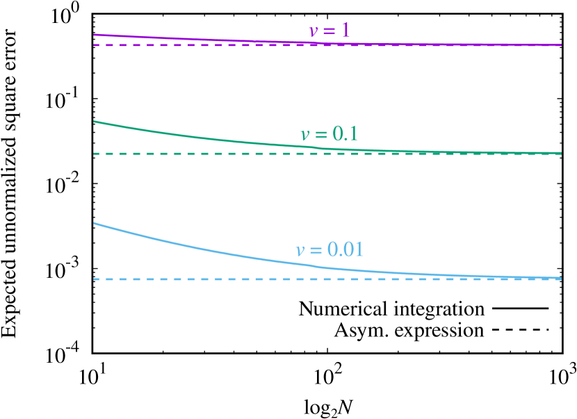
Figure 1: The expected unnormalized square error $\mathbb{E}[\|\boldsymbol{X}-f_{X}(\boldsymbol{Y};v_{\tilde{N}})\|_{2}^{2}]$ versus $\log_{2}N$ in Lemma 1 for $k=N^{0.25}$. The horizontal dashed lines show the asymptotic expression (17) in the sublinear sparsity limit.

V-B Linear Measurement

V-B1 State Evolution

We first verify the asymptotic expression (17) for the unnormalized square error in Lemma 1. Figure 1 shows the expected unnormalized square error $\mathbb{E}[\|\boldsymbol{X}-f_{X}(\boldsymbol{Y};v_{\tilde{N}})\|_{2}^{2}]$ with $v_{\tilde{N}}=v/\log(N/k)$. The expected unnormalized square error converges to the asymptotic expression (17) for all $v$ as $N$ increases. However, the convergence speed is extremely slow: We need $N=2^{1000}$ for the asymptotic expression to provide a good approximation for the expected unnormalized square error.

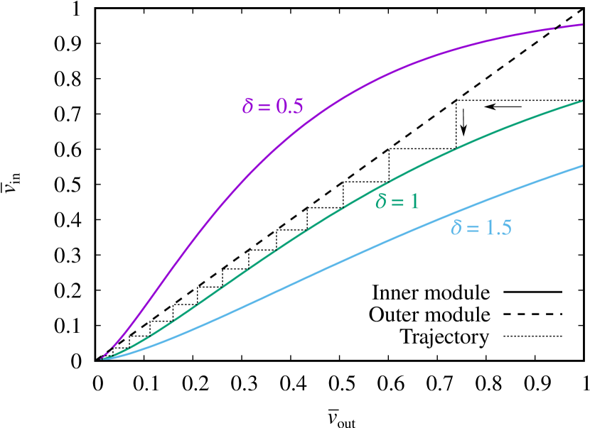
Figure 2: EXIT-like chart of Bayesian AMP for the linear measurement and $1/\sigma^{2}=40$ dB. The outer module shows the straight line (72) while the inner module represents (70) for $M/\{k\log(N/k)\}\to\delta$ in the sublinear sparsity limit. The chart is independent of the parameter $\log k/\log N\to\gamma\in[0,1)$.

We next focus on a chart to understand the dynamics of the state evolution recursion for the linear measurement, like the extrinsic information transfer (EXIT) chart. As shown in Fig. 2, $\bar{v}_{\mathrm{in},t}$ in (70) converges to the unique fixed point $\bar{v}_{\mathrm{in},\infty}\approx 0$ for $\delta=1$ and $\delta=1.5$ as $t\to\infty$. On the other hand, $\bar{v}_{\mathrm{in},t}$ tends to the fixed point in the upper right for $\delta=0.5$. Since the state evolution recursion (70) is a monotonically non-increasing function of $\delta$ for fixed $\bar{v}_{\mathrm{out},t}$, we arrive at the following definition of the weak reconstruction threshold:

Definition 4 (Weak Reconstruction Threshold)

The weak reconstruction threshold $\delta_{\mathrm{w}}^{*}>0$ for Bayesian AMP is defined as the infimum of $\delta^{\prime}$ such that the state evolution recursion (69) and (70) have a unique fixed point for all $\delta>\delta^{\prime}$.

The reconstruction threshold in Definition 3 requires exact signal reconstruction $\bar{v}_{\mathrm{in},\infty}=0$, as well as the uniqueness of the fixed point. The weak reconstruction threshold $\delta_{\mathrm{w}}^{*}$ indicates that the performance of Bayesian AMP changes discontinuously at $\delta=\delta_{\mathrm{w}}^{*}$.

V-B2 Numerical Simulation

Bayesian AMP was simulated for the linear measurement. As baselines, orthogonal matching pursuit (OMP) [70] and FISTA [10] were also simulated. FISTA is an iterative algorithm to solve the Lasso problem

$$\min_{\boldsymbol{x}\in\mathbb{R}^{N}}\frac{1}{2M}\|\boldsymbol{y}-\boldsymbol{A}\boldsymbol{x}\|_{2}^{2}+\lambda\|\boldsymbol{x}\|_{1}$$ (80)

for some $\lambda>0$. To improve the convergence property of FISTA, gradient-based restart [71] was used. Furthermore, the parameter $\lambda$ was optimized for each $\delta$ via exhaustive search to minimize the unnormalized square error in the last iteration.

Figure 3 shows the unnormalized square error of the three algorithms for the linear measurement. OMP has the error floor for large $\delta$ while it is comparable to Bayesian AMP around the weak reconstruction threshold. This observation is consistent to the fact that, once the position of non-zero signals is detected incorrectly, OMP has no procedure to correct the detection error.

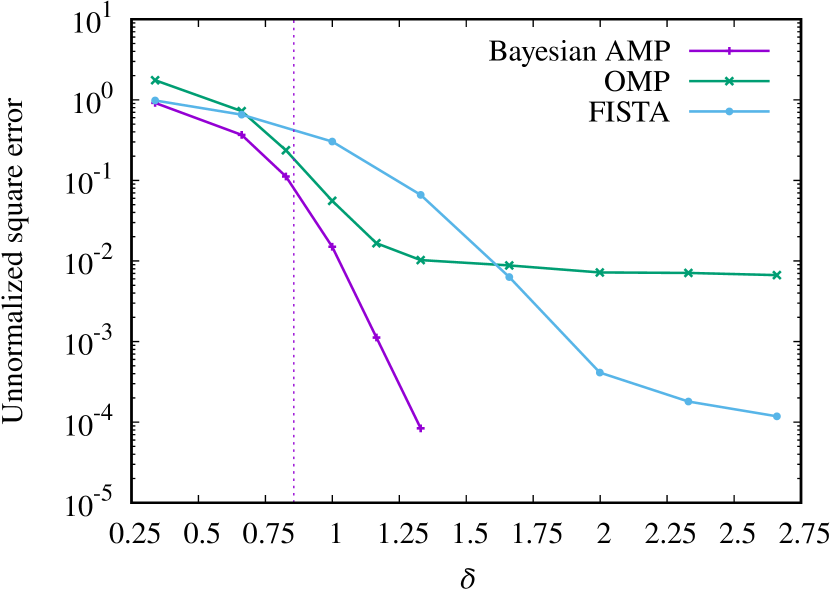
Figure 3: Unnormalized square error versus $\delta=M/\{k\log(N/k)\}$ for the linear measurement, $k=16$, $N=2^{16}$, and $1/\sigma^{2}=40$ dB. Bayesian AMP with $20$ iterations is compared to FISTA with backtracking [10], gradient-based restart [71], $10^{3}$ iterations, and optimized $\lambda$ in (80) for each $\delta$, as well as OMP [70] with $k$ iterations. The vertical dotted line shows the weak reconstruction threshold in Definition 4 for Bayesian AMP. $10^{4}$ independent trials were simulated for all algorithms, with the only exception of $10^{5}$ trials for Bayesian AMP with $\delta\approx 1.33$.

FISTA is inferior to Bayesian AMP while it achieves smaller unnormalized square error than OMP for large $\delta$. The poor performance of FISTA for large $\delta$ is due to its slow convergence: $10^{3}$ is not many iterations enough for FISTA to reach the true Lasso solution. Furthermore, FISTA is the worst among the three algorithms around the weak reconstruction threshold. This may be because FISTA uses no a priori information on the sparse signal vector.

Bayesian AMP achieves the best performance for all $\delta$. Interestingly, the weak reconstruction threshold provides a reasonably good prediction for the location of the so-called waterfall region for Bayesian AMP, in which the unnormalized square error decreases quickly as $\delta$ increases. This observation implies that qualitative changes, such as the number of fixed points for the state evolution recursion, are robust to the finite size effect, while the state evolution recursion cannot provide quantitatively reliable prediction for the unnormalized square error, as indicated from Fig. 1.

Figure 4 shows the convergence properties of the three algorithms. Bayesian AMP converges to a fixed point much more quickly than FISTA. The convergence speed of FISTA depends strongly on the parameter $\lambda$ in (80). Since $\lambda$ was optimized so as to minimize the unnormalized square error at the last iteration, FISTA converges slowly. If we used $\lambda$ smaller than the optimized value in Fig. 4, FISTA could not converge even after $10^{3}$ iterations. When we use larger $\lambda$, FISTA converges more quickly but cannot achieve the final unnormalized square error for the optimized value in Fig. 4.

V-C 1-bit Compressed Sensing

V-C1 State Evolution

We focus on 1-bit compressed sensing for the noiseless case $\sigma^{2}=0$. Figure 5 shows an EXIT-like chart for the state evolution recursion of Bayesian GAMP. The two curves for the outer and inner modules have two intersections $(\bar{v}_{\mathrm{out},\infty},\bar{v}_{\mathrm{in},\infty})$ at $\bar{v}_{\mathrm{out},\infty}=0$ and $\bar{v}_{\mathrm{out},\infty}>0$, of which the latter is the convergence point of the state evolution.

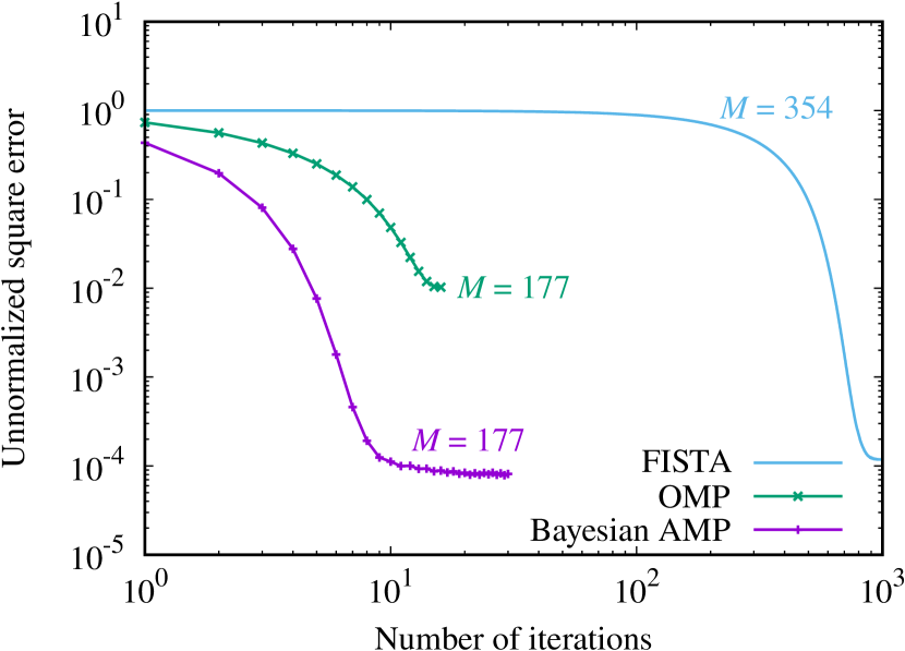
Figure 4: Unnormalized square error versus the number of iterations for the linear measurement, $k=16$, $N=2^{16}$, and $1/\sigma^{2}=40$ dB. Bayesian AMP is compared to OMP [70] and FISTA with backtracking [10], gradient-based restart [71], and optimized $\lambda=\sqrt{0.8\sigma^{2}M^{-1}\log N}$ [53]. $10^{5}$ independent trials were simulated for Bayesian AMP while $10^{4}$ independent trials were for OMP and FISTA.

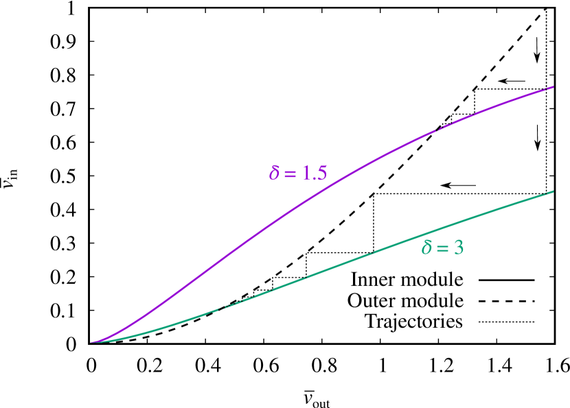
Figure 5: EXIT-like chart of Bayesian GAMP for 1-bit compressed sensing and $\sigma^{2}=0$. The outer module shows the inverse function of (78) while the inner module represents (70) for $M/\{k\log(N/k)\}\to\delta$ in the sublinear sparsity limit. The chart is independent of the parameter $\log k/\log N\to\gamma\in[0,1)$.

The EXIT-like chart for 1-bit compressed sensing is qualitatively different from that for the linear measurement in Fig. 2: Numerical evaluation implied that the state evolution recursion (70) and (78) have two fixed points for all $\delta>0$. In particular, the convergence point of Bayesian GAMP moves continuously toward the origin as $\delta$ increases. Thus, the reconstruction threshold in Definition 3 is $\delta^{*}=\infty$ for the sparse signal vector with non-zero Gaussian elements.

V-C2 Numerical Simulation

Bayesian GAMP was simulated for 1-bit compressed sensing in the noiseless case $\sigma^{2}=0$. As baselines, BIHT [22] and GLasso [23, 27] were also simulated. FISTA [10] was used to solve the Lasso problem (80) for GLasso. All algorithms converged quickly for 1-bit compressed sensing, as opposed to the linear measurement, so that $20$ iterations were used for all algorithms.

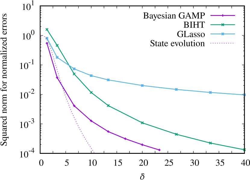
Figure 6: Squared norm (79) for the normalized error versus $\delta=M/\{k\log(N/k)\}$ for 1-bit compressed sensing, $k=16$, $N=2^{16}$, and $\sigma^{2}=0$. Bayesian GAMP is compared to BIHT [22] and GLasso [23, 27], as well as the state evolution for Bayesian GAMP. GLasso was implemented by using FISTA with backtracking [10], gradient-based restart [71], and optimized $\lambda$ in (80) for each $\delta$. $20$ iterations and $10^{4}$ independent trials were performed for all algorithms.

As shown in Fig. 6, Bayesian GAMP achieves the smallest squared norm (79) among the three algorithms. Interestingly, the state evolution result provides a reasonably accurate prediction for finite-sized systems when $\delta$ is small, while it cannot predict the occurrence of the error floor in the large $\delta$ regime. As a result, state evolution allows us to estimate roughly the location of waterfall region in which the squared norm (79) for the normalized error decreases rapidly.

VI Conclusions

This paper has proposed GAMP for reconstruction of an unknown signal vector with sublinear sparsity from the generalized linear measurement. State evolution has been used to evaluate the asymptotic dynamics of GAMP in terms of the unnormalized square error. The overall flow in state evolution is the same as that for the linear sparsity. To justify each proof step in state evolution. however, stronger assumptions for the inner denoiser are required than those for the linear sparsity. This paper has proved the required assumptions for the Bayesian inner denoiser. The state evolution and numerical results have implied that Bayesian GAMP is useful not only for the linear sparsity but also for the sublinear sparsity.

A challenge is to specify the class of inner denoisers that satisfy the last two assumptions in Assumption 7. These assumptions imply a smaller class than that of Lipschitz-continuous denoisers for the linear sparsity. Toward solving this challenging problem, a possible direction in future research would be to replace the Bayesian inner denoiser with the soft-thresholding denoiser.

Another challenge is finite size analysis of GAMP for the sublinear sparsity. As shown in Fig. 1, the sublinear sparsity limit needs too large systems to provide an accurate approximation for finite-sized systems. As a result, state evolution only provides a reasonably good prediction for the position of the reconstruction threshold. Finite size analysis would be able to provide an accurate prediction for the transient dynamics of GAMP for the sublinear sparsity.

Appendix A Proof of (22)

A-A Formulation

Prove the following more general result than (22):

$$(N-k)\mathbb{E}\left[|\Omega|^{j}f_{X}^{2}(\Omega;v_{\tilde{N}})\right]\to 0$$ (81)

for all non-negative integers $j\in\{0,1,\ldots\}$. The general result (81) is utilized in proving the other lemmas. We represent $\mathbb{E}[|\Omega|^{j}f_{X}^{2}(\Omega;v_{\tilde{N}})]$ with $\Omega\sim\mathcal{N}(0,v_{k,N})$ and $v_{k,N}=v_{\tilde{N}}/k$ as

$$\mathbb{E}[|\Omega|^{j}f_{X}^{2}(\Omega;v_{\tilde{N}})]=\int|w|^{j}f_{X}^{2}(w;v_{\tilde{N}})p_{\mathrm{G}}(w;v_{k,N})dw$$

$$=k^{-j/2}\int|\tilde{w}|^{j}f_{X}^{2}(k^{-1/2}\tilde{w};v_{\tilde{N}})p_{\mathrm{G}}(\tilde{w};v_{\tilde{N}})d\tilde{w}.$$ (82)

We decompose the interval of integration into three disjoint intervals,

$$\mathcal{W}_{1}=\{w\in\mathbb{R}:|w|<\sqrt{2\alpha_{N}v}\},$$ (83)

$$\mathcal{W}_{2}=\{w\in\mathbb{R}:|w|\in[\sqrt{2\alpha_{N}v},\sqrt{2v}]\},$$ (84)

$$\mathcal{W}_{3}=\{w\in\mathbb{R}:|w|>\sqrt{2v}\}$$ (85)

for $\alpha_{N}=1-\epsilon_{N}$ and $\epsilon_{N}=\log\log N/\log(N/k)$. In the following appendices we prove that the integral in (82) over each interval is $o((N-k)^{-1})$ in the sublinear sparsity limit.

In the interval $\mathcal{W}_{1}$ of integration, the posterior mean estimator $f_{A}(w;v_{\tilde{N}})$ is small enough to prove (81). In the interval $\mathcal{W}_{3}$ of integration, the probability $\mathrm{Pr}(|\tilde{\Omega}|>\sqrt{2v})$ for $\tilde{\Omega}\sim\mathcal{N}(0,v_{\tilde{N}})$ is small enough to prove (81). The remaining interval $\mathcal{W}_{2}$ corresponds to a thin transition interval between the two intervals.

A-B First Interval $\mathcal{W}_{1}$

We prove that the integral in (82) over $\mathcal{W}_{1}$ is $o((N-k)^{-1})$ in the sublinear sparsity limit. Using the definition of $f_{X}$ in (8) yields

$$k^{-j/2}\int_{\mathcal{W}_{1}}|w|^{j}f_{X}^{2}(k^{-1/2}w;v_{\tilde{N}})p_{\mathrm{G}}(w;v_{\tilde{N}})dw$$

$$\leq\frac{f_{U,\mathrm{max}_{1}}^{2}(v_{\tilde{N}})}{k^{1+j/2}}\int_{\mathcal{W}_{1}}|w|^{j}f_{A}^{2}(w;v_{\tilde{N}})p_{\mathrm{G}}(w;v_{\tilde{N}})dw,$$ (86)

with

$$f_{U,\mathrm{max}_{1}}(v_{\tilde{N}})=\sup_{w\in\mathcal{W}_{1}}|f_{U}(w;v_{\tilde{N}})|,$$ (87)

which is bounded for all $N$ because of the uniform Lipschitz-continuity assumption for $f_{U}$.

To evaluate the upper bound (86), we utilize an intuition in which $f_{A}$ should tend to zero in the sublinear sparsity limit for all $|w|<\sqrt{2\alpha_{N}v}$. In exploiting this intuition rigorously, we use the following upper bound for $f_{A}$ in (7):

$$f_{A}(w;v_{\tilde{N}}) <\frac{k\mathbb{E}_{U}[p_{\mathrm{G}}(w-U;v_{\tilde{N}})]}{(N-k)p_{\mathrm{G}}(w;v_{\tilde{N}})}$$

$$\leq\frac{k}{(N-k)\sqrt{2\pi v_{\tilde{N}}}p_{\mathrm{G}}(w;v_{\tilde{N}})}.$$ (88)

The last upper bound is slightly loose: For $U\sim\mathcal{N}(0,\sigma_{U}^{2})$ we have $\mathbb{E}_{U}[p_{\mathrm{G}}(w-U;v_{\tilde{N}})]=p_{\mathrm{G}}(y;\sigma_{U}^{2}+v_{\tilde{N}})\leq(2\pi\sigma_{U}^{2})^{-1/2}$ while the upper bound $\mathbb{E}_{U}[p_{\mathrm{G}}(w-U;v_{\tilde{N}})]\leq(2\pi v_{\tilde{N}})^{-1/2}$ has been used in (88). However, this loose bound is sufficient to prove Lemma 1.

We evaluate the upper bound (86). Applying the upper bound (88) to the integral in (86) yields

$$\frac{1}{k^{1+j/2}}\int_{\mathcal{W}_{1}}|w|^{j}f_{A}^{2}(w;v_{\tilde{N}})p_{\mathrm{G}}(w;v_{\tilde{N}})dw$$

$$<\frac{k^{1-j/2}}{(N-k)^{2}\sqrt{2\pi v_{\tilde{N}}}}\int_{\mathcal{W}_{1}}|w|^{j}\exp\left(\frac{w^{2}}{2v_{\tilde{N}}}\right)dw$$ (89)

$$\leq\frac{2k^{1-j/2}(2\alpha_{N}v)^{(j+1)/2}}{(N-k)^{2}\sqrt{2\pi v_{\tilde{N}}}}\exp\left(\frac{\alpha_{N}v}{v_{\tilde{N}}}\right)$$

$$=\frac{2\sqrt{\alpha_{N}}(2\alpha_{N}v)^{j/2}}{\sqrt{\pi}}\frac{k^{1-j/2}(N/k)^{\alpha_{N}}\sqrt{\log(N/k)}}{(N-k)^{2}},$$ (90)

with $v_{\tilde{N}}=v/\log(N/k)$. Combining these results, we arrive at

$$\frac{N-k}{k^{j/2}}\int_{\mathcal{W}_{1}}|w|^{j}f_{X}^{2}(k^{-1/2}w;v_{\tilde{N}})p_{\mathrm{G}}(w;v_{\tilde{N}})dw$$

$$<f_{U,\mathrm{max}_{1}}^{2}(v_{\tilde{N}})\frac{2\sqrt{\alpha_{N}}(2\alpha_{N}v)^{j/2}}{\sqrt{\pi}}$$

$$\cdot\frac{k^{1-j/2}(N/k)^{\alpha_{N}}\sqrt{\log(N/k)}}{N-k}\to 0$$ (91)

in the sublinear sparsity limit for all $j\geq 0$, because of $\alpha_{N}=1-\log\log N/\log(N/k)$.

A-C Second Interval $\mathcal{W}_{2}$

We prove that the integral in (82) over $\mathcal{W}_{2}$ is $o((N-k)^{-1})$ in the sublinear sparsity limit. Repeating the derivation of (89) yields

$$k^{-j/2}\int_{\mathcal{W}_{2}}|w|^{j}f_{X}^{2}(k^{-1/2}w;v_{\tilde{N}})p_{\mathrm{G}}(w;v_{\tilde{N}})dw$$

$$\leq\frac{2k^{1-j/2}f_{U,\mathrm{max}_{2}}^{2}(v_{\tilde{N}})}{(N-k)^{2}\sqrt{2\pi v_{\tilde{N}}}}\int_{\sqrt{2\alpha_{N}v}}^{\sqrt{2v}}|w|^{j}\exp\left(\frac{w^{2}}{2v_{\tilde{N}}}\right)dw$$ (92)

with

$$f_{U,\mathrm{max}_{2}}(v_{\tilde{N}})=\sup_{w\in\mathcal{W}_{2}}|f_{U}(w;v_{\tilde{N}})|,$$ (93)

which is bounded for all $N$ because of the uniform Lipschitz-continuity for $f_{U}$. Using the following upper bound:

$$\int_{\sqrt{2\alpha_{N}v}}^{\sqrt{2v}}|w|^{j}\exp\left(\frac{w^{2}}{2v_{\tilde{N}}}\right)dw$$

$$<(\sqrt{2v}-\sqrt{2\alpha_{N}v})(2v)^{j/2}\exp\left(\frac{v}{v_{\tilde{N}}}\right)$$

$$=\frac{(2v)^{(j+1)/2}}{1+\sqrt{\alpha_{N}}}\frac{k\log\log N}{N\log(N/k)}$$ (94)

for $\alpha_{N}=1-\log\log N/\log(N/k)$, we arrive at

$$\frac{N-k}{k^{j/2}}\int_{\mathcal{W}_{2}}|w|^{j}f_{X}^{2}(k^{-1/2}w;v_{\tilde{N}})p_{\mathrm{G}}(w;v_{\tilde{N}})dw$$

$$<\frac{2(2v)^{j/2}f_{U,\mathrm{max}_{2}}^{2}(v_{\tilde{N}})}{\sqrt{\pi}(1+\sqrt{\alpha_{N}})}\frac{k^{2-j/2}\log\log N}{(N-k)N\sqrt{\log(N/k)}}\to 0$$ (95)

in the sublinear sparsity limit for all $j\geq 0$.

A-D Last Interval $\mathcal{W}_{3}$

We prove that the integral in (82) over $\mathcal{W}_{3}$ is $o((N-k)^{-1})$ in the sublinear sparsity limit. We utilize an intuition in which the probability $\mathrm{Pr}(|\tilde{\Omega}|\geq\sqrt{2v})$ should tend to zero in the sublinear sparsity limit. This intuition allows us to bound $f_{X}^{2}$ roughly. Using the definition of $f_{X}(k^{-1/2}w;v_{\tilde{N}})$ in (8) and the trivial upper bound $f_{A}(w;v_{\tilde{N}})\leq 1$ yields

$$k^{-j/2}\int_{\mathcal{W}_{3}}|w|^{j}f_{X}^{2}(k^{-1/2}w;v_{\tilde{N}})p_{\mathrm{G}}(w;v_{\tilde{N}})dw$$

$$\leq\frac{1}{k^{1+j/2}}\int_{\mathcal{W}_{3}}|w|^{j}f_{U}^{2}(w;v_{\tilde{N}})p_{\mathrm{G}}(w;v_{\tilde{N}})dw.$$ (96)

The uniform Lipschitz-continuity assumption for $f_{U}$ implies that there are some $N$-independent constants $L>0$ and $C>0$ such that $|f_{U}(w;v_{\tilde{N}})|\leq L|w|+C$ holds for all $w\in\mathbb{R}$ and $N\in\mathbb{N}$. Thus, we have

$$\frac{1}{k^{1+j/2}}\int_{\mathcal{W}_{3}}|w|^{j}f_{U}^{2}(w;v_{\tilde{N}})p_{\mathrm{G}}(w;v_{\tilde{N}})dw$$

$$\leq\frac{2}{k^{1+j/2}}\int_{\sqrt{2v}}^{\infty}w^{j}(Lw+C)^{2}p_{\mathrm{G}}(w;v_{\tilde{N}})dw.$$ (97)

Contributions from $p_{\mathrm{G}}(w;v_{\tilde{N}})$ need to be evaluated carefully. Let

$$J_{j}=\int_{\sqrt{2v}}^{\infty}w^{j}p_{\mathrm{G}}(w;v_{\tilde{N}})dw.$$ (98)

We prove the following upper bound:

$$J_{j}<\frac{C_{j}k}{N\sqrt{\log(N/k)}}$$ (99)

for some constant $C_{j}>0$, which implies

$$\frac{N-k}{k^{j/2}}\int_{\mathcal{W}_{3}}|w|^{j}f_{X}^{2}(k^{-1/2}w;v_{\tilde{N}})p_{\mathrm{G}}(w;v_{\tilde{N}})dw$$

$$<\frac{2(L^{2}C_{j+2}+2LCC_{j+1}+C^{2}C_{j})(N-k)}{k^{j/2}N\sqrt{\log(N/k)}}\to 0$$ (100)

in the sublinear sparsity limit for all $j\geq 0$. Thus, (81) holds for all non-negative integers $j$.

To complete the proof of (100), we prove the upper bound (99) by induction. For $j=0$ we use the well-known upper bound $Q(x)<p_{\mathrm{G}}(x;1)/x$ on the Q-function for all $x>0$ to obtain

$$J_{0}=Q\left(\sqrt{2\log(N/k)}\right)<\frac{k}{2N\sqrt{\pi\log(N/k)}}.$$ (101)

For $j=1$ we have

$$J_{1}=[-v_{\tilde{N}}p_{\mathrm{G}}(w;v_{\tilde{N}})]_{\sqrt{2v}}^{\infty}=\frac{k}{N}\sqrt{\frac{v}{2\pi\log(N/k)}}.$$ (102)

Suppose that (99) is correct for some $j\geq 0$. Using the integration by parts for the indefinite integral $\int wp_{\mathrm{G}}(w;v_{\tilde{N}})dw=-v_{\tilde{N}}p_{\mathrm{G}}(w;v_{\tilde{N}})+{\rm Const.}$ yields

$$J_{j+2}=\left[-w^{j+1}v_{\tilde{N}}p_{\mathrm{G}}(w;v_{\tilde{N}})\right]_{\sqrt{2v}}^{\infty}+(j+1)v_{\tilde{N}}J_{j}$$

$$=\frac{(2v)^{(j+2)/2}k}{2N\sqrt{\pi\log(N/k)}}+\frac{(j+1)v}{\log(N/k)}J_{j}$$

$$<\left\{\frac{(2v)^{(j+2)/2}}{2\sqrt{\pi}}+\frac{(j+1)vC_{j}}{\log(N/k)}\right\}\frac{k}{N\sqrt{\log(N/k)}},$$ (103)

where the last inequality follows from the induction hypothesis (99). Thus, (99) holds for all non-negative integers $i$.

Appendix B Proof of (23)

B-A Influence of $f_{U}$

We evaluate the influence of $f_{U}$. Using the definition of $\Delta U(v_{\tilde{N}})$ in (24) and $\Omega\sim\mathcal{N}(0,v_{k,N})$ yields

$$\mathbb{E}\left[\Delta U^{2}(v_{\tilde{N}})\right]$$

$$=\mathbb{E}\left[\int\left\{U-\sqrt{k}f_{X}(k^{-1/2}U+w;v_{\tilde{N}})\right\}^{2}p_{\mathrm{G}}(w;v_{k,N})dw\right]$$

$$=\mathbb{E}\left[\int\left\{U-f_{A}(y;v_{\tilde{N}})f_{U}(y;v_{\tilde{N}})\right\}^{2}p_{\mathrm{G}}(y-U;v_{\tilde{N}})dy\right],$$ (104)

with $v_{k,N}=v_{\tilde{N}}/k$, where we have used the definition of $f_{X}$ in (8). Utilizing the following identity:

$$(U-f_{A}f_{U})^{2}=\{(1-f_{A})U+f_{A}(U-f_{U})\}^{2}$$

$$=(1-f_{A})^{2}U^{2}+2(1-f_{A})Uf_{A}(U-f_{U})+f_{A}^{2}(U-f_{U})^{2},$$ (105)

we have

$$\mathbb{E}\left[\Delta U^{2}(v_{\tilde{N}})\right]=\mathbb{E}\left[\int(1-f_{A})^{2}U^{2}p_{\mathrm{G}}(y-U;v_{\tilde{N}})dy\right]$$

$$+2\mathbb{E}\left[\int(1-f_{A})Uf_{A}(U-f_{U})p_{\mathrm{G}}(y-U;v_{\tilde{N}})dy\right]$$

$$+\mathbb{E}\left[\int f_{A}^{2}(U-f_{U})^{2}p_{\mathrm{G}}(y-U;v_{\tilde{N}})dy\right],$$ (106)

with $f_{A}=f_{A}(y;v_{\tilde{N}})$ and $f_{U}=f_{U}(y;v_{\tilde{N}})$.

We confirm that the second and last terms in (106) tend to zero in the sublinear sparsity limit. For the last term, using the trivial upper bound $f_{A}^{2}\leq 1$ and the change of variables $\tilde{y}=(y-U)/\sqrt{v_{\tilde{N}}}$ yields

$$\mathbb{E}\left[\int f_{A}^{2}(y;v_{\tilde{N}})\left\{U-f_{U}(y;v_{\tilde{N}})\right\}^{2}p_{\mathrm{G}}(y-U;v_{\tilde{N}})dy\right]$$

$$\leq\mathbb{E}\left[\int\left\{U-f_{U}(\sqrt{v_{\tilde{N}}}\tilde{y}+U;v_{\tilde{N}})\right\}^{2}p_{\mathrm{G}}(\tilde{y};1)d\tilde{y}\right].$$ (107)

The uniform Lipschitz-continuity for $f_{U}$ and the boundedness $\mathbb{E}[U^{2}]<\infty$ imply that the integrand is bounded from above by an $N$-independent and integrable function of $\{U,\tilde{y}\}$. Thus, we can use the reverse Fatou lemma to obtain

$$\limsup_{N\to\infty}\mathbb{E}\left[\int f_{A}^{2}\left(U-f_{U}\right)^{2}p_{\mathrm{G}}(y-U;v_{\tilde{N}})dy\right]$$

$$\leq\mathbb{E}\left[\int\limsup_{N\to\infty}\left\{U-f_{U}(\sqrt{v_{\tilde{N}}}\tilde{y}+U;v_{\tilde{N}})\right\}^{2}p_{\mathrm{G}}(\tilde{y};1)d\tilde{y}\right]$$

$$=\mathbb{E}\left[\limsup_{N\to\infty}\left\{U-f_{U}(U;v_{\tilde{N}})\right\}^{2}\right]=0$$ (108)

in the sublinear sparsity limit, where the last equality follows from the consistency $\lim_{v\to 0}f_{U}(u;v)=u$. Using the upper bound $|(1-f_{A})Uf_{A}(U-f_{U})|<|U(U-f_{U})|$ and repeating the same proof, we find that the second term in (106) tends to zero in the sublinear sparsity limit.

B-B Formulation

It is sufficient to prove that the first term in (106) converges to the right-hand side (RHS) of (23) in the sublinear sparsity limit. We decompose the interval of integration into three disjoint intervals,

$$\mathcal{Y}_{1}=\left\{y\in\mathbb{R}:|y|<\sqrt{2\alpha_{N}v}\right\},$$ (109)

$$\mathcal{Y}_{2}=\left\{y\in\mathbb{R}:|y|\in[\sqrt{2\alpha_{N}v},\sqrt{2\beta_{N}v}]\right\},$$ (110)

$$\mathcal{Y}_{3}=\left\{y\in\mathbb{R}:|y|>\sqrt{2\beta_{N}v}\right\}$$ (111)

for $\epsilon_{N}=\log\log N/\log(N/k)$, $\alpha_{N}=1-\epsilon_{N}$, and $\beta_{N}=1+\epsilon_{N}$. In the following appendices we prove that the integral over $\mathcal{Y}_{1}$ converges to the RHS of (23) in the sublinear sparsity limit while the integrals over $\mathcal{Y}_{2}$ and $\mathcal{Y}_{3}$ are proved to be zero.

In the interval $\mathcal{Y}_{1}$ of integration, $f_{A}(y;v_{\tilde{N}})$ is negligibly small. This false negative event contributes to the unnormalized square error. In the interval $\mathcal{Y}_{3}$ of integration, $f_{A}(y;v_{\tilde{N}})$ tends to $1$ with the exception of negligibly rare events. The remaining interval $\mathcal{Y}_{2}$ corresponds to a thin transition interval between the two intervals.

B-C First Interval $\mathcal{Y}_{1}$

We evaluate the integral for the first term in (106) over $\mathcal{Y}_{1}$. Using the change of variables $\tilde{y}=(y-U)/\sqrt{v_{\tilde{N}}}$ yields

$$\mathbb{E}\left[\int_{\mathcal{Y}_{1}}\{1-f_{A}(y;v_{\tilde{N}})\}^{2}U^{2}p_{\mathrm{G}}(y-U;v_{\tilde{N}})dy\right]$$

$$=\mathbb{E}\left[\int F(\sqrt{v_{\tilde{N}}}\tilde{y}+U;v_{\tilde{N}})U^{2}p_{\mathrm{G}}(\tilde{y};1)d\tilde{y}\right],$$ (112)

with

$$F(y;v_{\tilde{N}})=1(y\in\mathcal{Y}_{1})\{1-f_{A}(y;v_{\tilde{N}})\}^{2}.$$ (113)

To use the dominated convergence theorem, we first observe that the integrand in (112) is bounded from above by integrable $U^{2}p_{\mathrm{G}}(\tilde{y};1)$, because of $F(y;v_{\tilde{N}})\leq 1$ and $\mathbb{E}[U^{2}]<\infty$. We next need to prove that $f_{A}(y;v_{\tilde{N}})$ converges uniformly to zero for all $|y|<\sqrt{2\alpha_{N}v}$ in the sublinear sparsity limit. This uniform convergence implies the almost sure convergence $F(\sqrt{v_{\tilde{N}}}\tilde{y}+U;v_{\tilde{N}})\overset{\mathrm{a.s.}}{\to}1(|U|<\sqrt{2v})$ for all $|\sqrt{v}_{N}\tilde{y}+U|<\sqrt{2\alpha_{N}v}$, because of $\alpha_{N}=1-\log\log N/\log(N/k)\to 1$. These observations allow us to use the dominated convergence theorem to arrive at

$$\lim_{N\to\infty}\mathbb{E}\left[\int_{\mathcal{Y}_{1}}\{1-f_{A}(y;v_{\tilde{N}})\}^{2}U^{2}p_{\mathrm{G}}(y-U;v_{\tilde{N}})dy\right]$$

$$=\mathbb{E}\left[\int\lim_{N\to\infty}F(\sqrt{v_{\tilde{N}}}\tilde{y}+U;v_{\tilde{N}})U^{2}p_{\mathrm{G}}(\tilde{y};1)d\tilde{y}\right]$$

$$=\mathbb{E}\left[U^{2}1(|U|<\sqrt{2v})\right]$$ (114)

in the sublinear sparsity limit, which is equal to the RHS of (23).

To justify the use of the dominated convergence theorem, we prove that $f_{A}(y;v_{\tilde{N}})$ converges uniformly to zero for all $|y|<\sqrt{2\alpha_{N}v}$ in the sublinear sparsity limit. Using the definition of $f_{A}$ in (7) yields

$$f_{A}(y;v_{\tilde{N}})<\frac{k\mathbb{E}_{U}[e^{-(y-U)^{2}/(2v_{\tilde{N}})}]}{(N-k)e^{-y^{2}/(2v_{\tilde{N}})}}<\frac{k(N/k)^{\alpha_{N}}}{N-k}$$ (115)

for all $|y|<\sqrt{2\alpha_{N}v}$. Thus, for $\alpha_{N}=1-\log\log N/\log(N/k)$ we find that $f_{A}(y;v_{\tilde{N}})$ converges uniformly to zero for all $|y|<\sqrt{2\alpha_{N}v}$ in the sublinear sparsity limit.

B-D Second Interval $\mathcal{Y}_{2}$

We prove that the integral for the first term in (106) over $\mathcal{Y}_{2}$ tends to zero in the sublinear sparsity limit. Applying the change of variables $y^{\prime}=-y$ for the negative interval $y\in[-\sqrt{2\beta_{N}v},-\sqrt{2\alpha_{N}v}]$ yields

$$\mathbb{E}\left[\int_{\mathcal{Y}_{2}}(1-f_{A})^{2}U^{2}p_{\mathrm{G}}(y-U;v_{\tilde{N}})dy\right]$$

$$=\mathbb{E}\left[\int_{\sqrt{2\alpha_{N}v}}^{\sqrt{2\beta_{N}v}}\{1-f_{A}(y;v_{\tilde{N}})\}^{2}U^{2}p_{\mathrm{G}}(y-U;v_{\tilde{N}})dy\right]$$

$$+\mathbb{E}\left[\int_{\sqrt{2\alpha_{N}v}}^{\sqrt{2\beta_{N}v}}\{1-f_{A}(-y^{\prime};v_{\tilde{N}})\}^{2}U^{2}p_{\mathrm{G}}(y^{\prime}+U;v_{\tilde{N}})dy^{\prime}\right].$$ (116)

We only prove the convergence of the first term in (116) to zero since the second term can be evaluated in the same manner.

We use the upper bound $(1-f_{A})^{2}\leq 1$ and the change of variables $y=(2v+2v_{\tilde{N}}z)^{1/2}\equiv y(z)$ to evaluate the first term in (116) as

$$\mathbb{E}\left[\int_{\sqrt{2\alpha_{N}v}}^{\sqrt{2\beta_{N}v}}\{1-f_{A}(y;v_{\tilde{N}})\}^{2}U^{2}p_{\mathrm{G}}(y-U;v_{\tilde{N}})dy\right]$$

$$\leq\mathbb{E}\left[\int_{-\epsilon_{N}\log(N/k)}^{\epsilon_{N}\log(N/k)}\frac{\sqrt{v_{\tilde{N}}}U^{2}p_{\mathrm{G}}(y(z)-U;v_{\tilde{N}})}{\sqrt{2\{\log(N/k)+z\}}}dz\right]$$ (117)

for $\alpha_{N}=1-\epsilon_{N}$ and $\beta_{N}=1+\epsilon_{N}$. From the definition of $y(z)$, for $|z|\leq\epsilon_{N}\log(N/k)$ we have

$$\log\left\{\sqrt{2\pi v_{\tilde{N}}}p_{\mathrm{G}}(y(z)-U;v_{\tilde{N}})\right\}$$

$$=U\left\{\frac{2}{v}\left[1+\frac{z}{\log(N/k)}\right]\right\}^{1/2}\log(N/k)-z$$

$$-\left(1+\frac{U^{2}}{2v}\right)\log(N/k)\leq\frac{\tilde{U}}{\sqrt{2v}}z-\frac{\tilde{U}^{2}}{2v}\log(N/k),$$ (118)

with $\tilde{U}=U-\sqrt{2v}$, where the inequality follows from the upper bound $\sqrt{1+x}\leq 1+x/2$ for all $x\in[-1,\infty)$. Applying the upper bound (118) into (117) yields

$$\mathbb{E}\left[\int_{\sqrt{2\alpha_{N}v}}^{\sqrt{2\beta_{N}v}}\{1-f_{A}(y;v_{\tilde{N}})\}^{2}U^{2}p_{\mathrm{G}}(y-U;v_{\tilde{N}})dy\right]$$

$$<\mathbb{E}\left[\frac{U^{2}(N/k)^{-\tilde{U}^{2}/(2v)}}{2\sqrt{\pi(1-\epsilon_{N})\log(N/k)}}\int_{-\epsilon_{N}\log(N/k)}^{\epsilon_{N}\log(N/k)}e^{\frac{\tilde{U}z}{\sqrt{2v}}}dz\right].$$ (119)

To upper-bound (119), we use the following upper bound:

$$\int_{-\epsilon_{N}\log(N/k)}^{\epsilon_{N}\log(N/k)}e^{\frac{\tilde{U}z}{\sqrt{2v}}}dz\leq 2\left(\frac{N}{k}\right)^{\frac{|\tilde{U}|\epsilon_{N}}{\sqrt{2v}}}\epsilon_{N}\log(N/k),$$ (120)

which is tight for $\tilde{U}=0$. Applying this upper bound to (119), we arrive at

$$\mathbb{E}\left[\int_{\sqrt{2\alpha_{N}v}}^{\sqrt{2\beta_{N}v}}\{1-f_{A}(y;v_{\tilde{N}})\}^{2}U^{2}p_{\mathrm{G}}(y-U;v_{\tilde{N}})dy\right]$$

$$<\mathbb{E}\left[U^{2}\epsilon_{N}\sqrt{\frac{\log(N/k)}{\pi(1-\epsilon_{N})}}\left(\frac{N}{k}\right)^{\frac{|\tilde{U}|\epsilon_{N}}{\sqrt{2v}}-\frac{\tilde{U}^{2}}{2v}}\right]$$

$$\leq\epsilon_{N}\left(\frac{N}{k}\right)^{\epsilon_{N}^{2}/4}\sqrt{\frac{\log(N/k)}{\pi(1-\epsilon_{N})}}\mathbb{E}[U^{2}]\to 0$$ (121)

in the sublinear sparsity limit for $\epsilon_{N}=\log\log N/\log(N/k)$. In the derivation of the second inequality, we have used the following elementary upper bound:

$$\max_{\tilde{u}\in\mathbb{R}}\left(\frac{|\tilde{u}|\epsilon_{N}}{\sqrt{2v}}-\frac{\tilde{u}^{2}}{2v}\right)\leq\frac{\epsilon_{N}^{2}}{4},$$ (122)

where the equality is attained at $|\tilde{u}|=\epsilon_{N}\sqrt{v/2}$.

B-E Last Interval $\mathcal{Y}_{3}$

B-E1 Noise Truncation

We prove that the integral for the first term in (106) over $\mathcal{Y}_{3}$ tends to zero in the sublinear sparsity limit. Using the change of variables $w=y-U$ yields

$$\mathbb{E}\left[\int_{\mathcal{Y}_{3}}\{1-f_{A}(y;v_{\tilde{N}})\}^{2}U^{2}p_{\mathrm{G}}(y-U;v_{\tilde{N}})dy\right]$$

$$=\mathbb{E}\left[\int_{\mathcal{W}_{1}(U)}\{1-f_{A}(U+w;v_{\tilde{N}})\}^{2}U^{2}p_{\mathrm{G}}(w;v_{\tilde{N}})dw\right]$$

$$+\mathbb{E}\left[\int_{\mathcal{W}_{2}(U)}\{1-f_{A}(U+w;v_{\tilde{N}})\}^{2}U^{2}p_{\mathrm{G}}(w;v_{\tilde{N}})dw\right],$$ (123)

with

$$\mathcal{W}_{1}(u)=\{w\in\mathbb{R}:|w|\leq\sqrt{\epsilon_{N}v},|u+w|>\sqrt{2\beta_{N}v}\},$$ (124)

$$\mathcal{W}_{2}(u)=\{w\in\mathbb{R}:|w|>\sqrt{\epsilon_{N}v},|u+w|>\sqrt{2\beta_{N}v}\}.$$ (125)

The set $\mathcal{W}_{2}(u)$ contains too rare noise samples to contribute to the unnormalized square error. Thus, the main challenge is evaluation of the first term in (123) that depends on the set of the remaining noise samples $\mathcal{W}_{1}(u)$.

We confirm that the second term in (123) tends to zero in the sublinear sparsity limit. Using the trivial upper bound $(1-f_{A})^{2}\leq 1$ and $\mathcal{W}_{2}(u)\subset\{w\in\mathbb{R}:|w|>\sqrt{\epsilon_{N}v}\}$ yields

$$\mathbb{E}\left[\int_{\mathcal{W}_{2}(U)}\{1-f_{A}(U+w;v_{\tilde{N}})\}^{2}U^{2}p_{\mathrm{G}}(w;v_{\tilde{N}})dw\right]$$

$$<\mathbb{E}[U^{2}]\int_{|w|>\sqrt{\epsilon_{N}v}}p_{\mathrm{G}}(w;v_{\tilde{N}})dw$$

$$=2\mathbb{E}[U^{2}]Q\left(\sqrt{\epsilon_{N}\log(N/k)}\right).$$ (126)

We utilize the upper bound $Q(x)<p_{\mathrm{G}}(x;1)/x$ on the Q-function for all $x>0$ to obtain

$$\mathbb{E}\left[\int_{\mathcal{W}_{2}(U)}\{1-f_{A}(U+w;v_{\tilde{N}})\}^{2}U^{2}p_{\mathrm{G}}(w;v_{\tilde{N}})dw\right]$$

$$<\frac{2\mathbb{E}[U^{2}](N/k)^{-\epsilon_{N}/2}}{\sqrt{2\pi\epsilon_{N}\log(N/k)}}\to 0$$ (127)

in the sublinear sparsity limit for $\epsilon_{N}=\log\log N/\log(N/k)$.

To evaluate the first term in (123), we use the assumption for the cumulative distribution of $U$, which implies that the pdf of $U$ is given by

$$p_{U}(u)=\sum_{i=1}^{\infty}p_{U,i}^{\mathrm{D}}\delta(u-u_{i})+(1-p_{U}^{\mathrm{D}})p_{U}^{\mathrm{C}}(u),$$ (128)

with

$$p_{U}^{\mathrm{D}}=\sum_{i=1}^{\infty}p_{U,i}^{\mathrm{D}}\in[0,1],\quad p_{U,i}^{\mathrm{D}}\geq 0.$$ (129)

In the discrete components of (128), $p_{U,i}^{\mathrm{D}}\in[0,1]$ denotes the probability with which $U$ takes $u_{i}$.

In the continuous component, the pdf $p_{U}^{\mathrm{C}}(u)$ with a support $\mathcal{S}_{U}^{\mathrm{C}}=\{u\in\mathbb{R}:p_{U}^{\mathrm{C}}(u)>0\}$ is almost everywhere continuous. Since $\mathcal{S}_{U}^{\mathrm{C}}$ is a Borel set on $\mathbb{R}$, without loss of generality, the support $\mathcal{S}_{U}^{\mathrm{C}}$ can be decomposed into the union of countable and disjoint intervals,

$$\mathcal{S}_{U}^{\mathrm{C}}=\cup_{i\in\mathbb{N}}\mathcal{S}_{U,i}^{\mathrm{C}},$$ (130)

where disjoint intervals $\{\mathcal{S}_{U,i}^{\mathrm{C}}\subset\mathbb{R}\}$ satisfy $\mathcal{S}_{U,i}^{\mathrm{C}}\cap\mathcal{S}_{U,j}^{\mathrm{C}}=\emptyset$ for all $i\neq j$.

We focus on the discrete case $p_{U}^{\mathrm{D}}=1$ and the case $p_{U}^{\mathrm{D}}<1$, of which the latter is separated into two cases: In one case—called the discrete-continuous mixture case—part of discrete components $\{u_{i}\}$ are outside the support $\mathcal{S}_{U}^{\mathrm{C}}$ of the continuous component. In the other case—called the continuous case—there are no discrete components outside the support $\mathcal{S}_{U}^{\mathrm{C}}$. We consider these three cases separately.

B-E2 Discrete Case

Assume $p_{U}^{\mathrm{D}}=1$. We derive the set of $y\in\mathbb{R}$ such that $f_{A}(y;v_{\tilde{N}})$ tends to $1$ in the sublinear sparsity limit. Using the definition of $f_{A}$ in (7) yields

$$f_{A}(y;v_{\tilde{N}})=\left\{1+\frac{(N-k)(N/k)^{-y^{2}/(2v)}}{k\mathbb{E}_{U}[(N/k)^{-(y-U)^{2}/(2v)}]}\right\}^{-1}.$$ (131)

Applying the pdf (128) of $U$ with $p_{\mathrm{D}}=1$, we have

$$\mathbb{E}_{U}[(N/k)^{-(y-U)^{2}/(2v)}]=\sum_{i=1}^{\infty}p_{U,i}^{\mathrm{D}}\left(\frac{N}{k}\right)^{-\frac{(y-u_{i})^{2}}{2v}}$$

$$>p_{U,i(y)}^{\mathrm{D}}\left(\frac{N}{k}\right)^{-\frac{(y-u_{i(y)})^{2}}{2v}}>\left(\frac{N}{k}\right)^{-\frac{\epsilon_{N}}{4}-\frac{(y-u_{i(y)})^{2}}{2v}}$$ (132)

for $\epsilon_{N}=\log\log N/\log(N/k)$, with

$$i(y)=\mathop{\mathrm{argmin}}\limits_{i\in\mathbb{N}:p_{U,i}^{\mathrm{D}}>(N/k)^{-\epsilon_{N}/4}}(y-u_{i})^{2}.$$ (133)

Note that this minimization problem is feasible for the discrete case $p_{U}^{\mathrm{D}}=1$.

We prove $f_{A}(y;v_{\tilde{N}})\to 1$ when $y^{2}-(y-u_{i(y)})^{2}>(2+\epsilon_{N})v$ holds. Using the lower bound (132) yields

$$\frac{(N-k)(N/k)^{-y^{2}/(2v)}}{k\mathbb{E}_{U}[(N/k)^{-(y-U)^{2}/(2v)}]} <\frac{(N/k)^{1-y^{2}/(2v)}}{(N/k)^{-\epsilon_{N}/4-(y-u_{i(y)})^{2}/(2v)}}$$

$$<(N/k)^{-\epsilon_{N}/4}$$ (134)

for $y^{2}-(y-u_{i(y)})^{2}>(2+\epsilon_{N})v$. Applying this upper bound to (131), we arrive at

$$f_{A}(y;v_{\tilde{N}})>\frac{1}{1+(N/k)^{-\epsilon_{N}/4}}$$ (135)

for all $\{y\in\mathbb{R}:(y-u_{i(y)})^{2}<y^{2}-(2+\epsilon_{N})v\}$, which tends to $1$ in the sublinear sparsity limit for $\epsilon_{N}=\log\log N/\log(N/k)$.

We evaluate the first term in (123). Utilizing the lower bound on $f_{A}$ in (135) yields

$$\limsup_{N\to\infty}\mathbb{E}\left[\int_{\mathcal{W}_{1}(U)}\left\{1-f_{A}(U+w;v_{\tilde{N}})\right\}^{2}U^{2}p_{\mathrm{G}}(w;v_{\tilde{N}})dw\right]$$

$$=\limsup_{N\to\infty}\mathbb{E}\left[\int_{\mathcal{W}_{1}(U)}\left\{1-f_{A}(U+w;v_{\tilde{N}})\right\}^{2}U^{2}p_{\mathrm{G}}(w;v_{\tilde{N}})\right.$$

$$\cdot 1\left((U+w-u_{i(U+w)})^{2}\geq(U+w)^{2}-(2+\epsilon_{N})v\right)dw\bigg{]}$$ (136)

in the sublinear sparsity limit. Applying the upper bound $(1-f_{A})^{2}\leq 1$ and the pdf of $U$ in (128) with $p_{U}^{\mathrm{D}}=1$, we have

$$\limsup_{N\to\infty}\mathbb{E}\left[\int_{\mathcal{W}_{1}(U)}\left\{1-f_{A}(U+w;v_{\tilde{N}})\right\}^{2}U^{2}p_{\mathrm{G}}(w;v_{\tilde{N}})dw\right]$$

$$\leq\sum_{j=1}^{\infty}\limsup_{N\to\infty}p_{U,j}^{\mathrm{D}}u_{j}^{2}\int_{\mathcal{W}_{1}(u_{j})}p_{\mathrm{G}}(w;v_{\tilde{N}})$$

$$\cdot 1\left((u_{j}+w-u_{i(u_{j}+w)})^{2}\geq(u_{j}+w)^{2}-(2+\epsilon_{N})v\right)dw,$$ (137)

where we have used the reverse Fatou lemma since the terms in the summation are bounded from above by summable $\{p_{U,j}^{\mathrm{D}}u_{j}^{2}\}$.

We prove that the upper bound (137) is equal to zero. Let $\mathcal{I}=\{i\in\mathbb{N}:p_{U,i}^{\mathrm{D}}>(N/k)^{-\epsilon_{N}/4}\}$. Since $p_{U,j}^{\mathrm{D}}$ tends to zero in the sublinear sparsity limit for all $j\notin\mathcal{I}$, (137) reduces to

$$\limsup_{N\to\infty}\mathbb{E}\left[\int_{\mathcal{W}_{1}(U)}\left\{1-f_{A}(U+w;v_{\tilde{N}})\right\}^{2}U^{2}p_{\mathrm{G}}(w;v_{\tilde{N}})dw\right]$$

$$\leq\sum_{j\in\mathcal{I}}\limsup_{N\to\infty}p_{U,j}^{\mathrm{D}}u_{j}^{2}\int_{\mathcal{W}_{1}(u_{j})\cap\mathcal{W}_{\mathrm{d}}(u_{j})}p_{\mathrm{G}}(w;v_{\tilde{N}})dw,$$ (138)

with

$$\mathcal{W}_{\mathrm{d}}(u)=\left\{w\in\mathbb{R}:(u+w)^{2}\leq w^{2}+(2+\epsilon_{N})v\right\},$$ (139)

where we have used the following upper bound obtained from the definition of $i(y)$ in (133):

$$\left(u_{j}+w-u_{i(u_{j}+w)}\right)^{2}\leq(u_{j}+w-u_{j})^{2}=w^{2}$$ (140)

for all $j\in\mathcal{I}$. The two sets $\mathcal{W}_{1}(u_{j})$ in (124) and $\mathcal{W}_{\mathrm{d}}(u_{j})$ in (139) have no intersection since $|w|\leq\sqrt{\epsilon_{N}v}$ in (124) yields

$$w^{2}+(2+\epsilon_{N})v\leq 2(1+\epsilon_{N})v=2\beta_{N}v.$$ (141)

This observation implies that (138) is equal to zero. Thus, the first term in (123) tends to zero in the sublinear sparsity limit for $p_{U}^{\mathrm{D}}=1$.

B-E3 Discrete-Continuous Mixture Case

Assume $p_{U}^{\mathrm{D}}<1$. We prove $f_{A}(y;v_{\tilde{N}})\to 1$ almost everywhere for $\{y\in\mathcal{S}_{U}^{\mathrm{C}}:|y|>\sqrt{2\beta_{N}v}\}$. Using definition of $f_{A}(y;v_{\tilde{N}})$ in (7) yields

$$f_{A}(y;v_{\tilde{N}})=\left(1+\frac{k^{-1}(N-k)p_{\mathrm{G}}(y;v_{\tilde{N}})}{\mathbb{E}_{U}[p_{\mathrm{G}}(y-U;v_{\tilde{N}})]}\right)^{-1}.$$ (142)

To lower-bound $f_{A}(y;v_{\tilde{N}})$, for the numerator we have

$$k^{-1}(N-k)p_{\mathrm{G}}(y;v_{\tilde{N}})<\frac{1}{\sqrt{2\pi v_{\tilde{N}}}}\left(\frac{N}{k}\right)^{1-\beta_{N}}$$ (143)

for all $|y|>\sqrt{2\beta_{N}v}$, which tends to zero in the sublinear sparsity limit for $\beta_{N}=1+\log\log N/\log(N/k)$. On the other hand, using the pdf (128) for the denominator yields

$$\mathbb{E}_{U}[p_{\mathrm{G}}(y-U;v_{\tilde{N}})]\geq(1-p_{U}^{\mathrm{D}})\int p_{\mathrm{G}}(y-u;v_{\tilde{N}})p_{U}^{\mathrm{C}}(u)du.$$ (144)

We use the change of variables $\tilde{u}=(u-y)/\sqrt{v_{\tilde{N}}}$ and Fatou’s lemma to obtain

$$\liminf_{N\to\infty}\mathbb{E}_{U}[p_{\mathrm{G}}(y-U;v_{\tilde{N}})]$$

$$\geq(1-p_{U}^{\mathrm{D}})\int p_{\mathrm{G}}(\tilde{u};1)\liminf_{N\to\infty}p_{U}^{\mathrm{C}}(\sqrt{v_{\tilde{N}}}\tilde{u}+y)d\tilde{u}$$

$$=(1-p_{U}^{\mathrm{D}})p_{U}^{\mathrm{C}}(y)~{}\hbox{almost everywhere}$$ (145)

in the sublinear sparsity limit, where the last equality follows from the almost everywhere continuity of $p_{U}^{\mathrm{C}}(u)$. In particular, the lower bound (145) is strictly positive for all $y\in\mathcal{S}_{U}^{\mathrm{C}}$. Combining these results, we find that $f_{A}(y;v_{\tilde{N}})$ converges almost everywhere to $1$ for $\{y\in\mathcal{S}_{U}^{\mathrm{C}}:|y|>\sqrt{2\beta_{N}v}\}$ in the sublinear sparsity limit.

We evaluate the first term in (123). Since we have proved $f_{A}(y;v_{\tilde{N}})\to 1$ almost everywhere for the continuous component, we obtain

$$\lim_{N\to\infty}\mathbb{E}\left[\int_{\mathcal{W}_{1}(U)}\{1-f_{A}(U+w;v_{\tilde{N}})\}^{2}U^{2}p_{\mathrm{G}}(w;v_{\tilde{N}})dw\right]$$

$$=\lim_{N\to\infty}\mathbb{E}\left[\int_{\tilde{\mathcal{W}}_{1}(U)}\{1-f_{A}(U+w;v_{\tilde{N}})\}^{2}U^{2}p_{\mathrm{G}}(w;v_{\tilde{N}})dw\right]$$ (146)

in the sublinear sparsity limit, with

$$\tilde{\mathcal{W}}_{1}(u)=\{w:u+w\notin\mathcal{S}_{U}^{\mathrm{C}},|w|\leq\sqrt{\epsilon_{N}v},|u+w|>\sqrt{2\beta_{N}v}\}.$$ (147)

When there is some discrete component $u_{i}$ in (128) such that $\tilde{\mathcal{W}}_{1}(u_{i})\neq\emptyset$ holds, we repeat the proof for the discrete case $p_{U}^{\mathrm{D}}=1$ to find that (146) tends to zero in the sublinear sparsity limit.

B-E4 Continuous Case

Assume $p_{U}^{\mathrm{D}}=0$ or $\tilde{\mathcal{W}}_{1}(u_{i})=\emptyset$ for all $i\in\mathbb{N}$. We use the pdf of $U$ in (128) and the upper bound $(1-f_{A})^{2}\leq 1$ to evaluate (146) as

$$\mathbb{E}\left[\int_{\tilde{\mathcal{W}}_{1}(U)}\{1-f_{A}(U+w;v_{\tilde{N}})\}^{2}U^{2}p_{\mathrm{G}}(w;v_{\tilde{N}})dw\right]$$

$$\leq(1-p_{U}^{\mathrm{D}})\int_{\mathcal{S}_{U}^{\mathrm{C}}}u^{2}p_{U}^{\mathrm{C}}(u)du\int_{\tilde{\mathcal{W}}_{1}(u)}p_{\mathrm{G}}(w;v_{\tilde{N}})dw$$

$$=(1-p_{U}^{\mathrm{D}})\sum_{i\in\mathbb{N}}\int_{\mathcal{S}_{U,i}^{\mathrm{C}}}u^{2}p_{U}^{\mathrm{C}}(u)du\int_{\tilde{\mathcal{W}}_{1}(u)}p_{\mathrm{G}}(w;v_{\tilde{N}})dw,$$ (148)

where the last equality follows from the support representation (130). Let $\tilde{\mathcal{S}}_{U,i}^{\mathrm{C}}=\{u\in\mathcal{S}_{U,i}^{\mathrm{C}}:u+w\in\mathcal{S}_{U}^{\mathrm{C}}~{}\hbox{for all $|w|\leq\sqrt{\epsilon_{N}v}$}\}$ denote a subset of the interior of $\mathcal{S}_{U,i}^{\mathrm{C}}$. We find $\tilde{\mathcal{W}}_{1}(u)=\emptyset$ in (147) for all $u\in\tilde{\mathcal{S}}_{U,i}^{\mathrm{C}}$ to obtain

$$\sum_{i\in\mathbb{N}}\int_{\mathcal{S}_{U,i}^{\mathrm{C}}}u^{2}p_{U}^{\mathrm{C}}(u)du\int_{\tilde{\mathcal{W}}_{1}(u)}p_{\mathrm{G}}(w;v_{\tilde{N}})dw$$

$$=\sum_{i\in\mathbb{N}}\int_{\partial\mathcal{S}_{U,i}^{\mathrm{C}}}u^{2}p_{U}^{\mathrm{C}}(u)du\int_{\tilde{\mathcal{W}}_{1}(u)}p_{\mathrm{G}}(w;v_{\tilde{N}})dw$$

$$<\sum_{i\in\mathbb{N}}\int_{\partial\mathcal{S}_{U,i}^{\mathrm{C}}}u^{2}p_{U}^{\mathrm{C}}(u)du,$$ (149)

with $\partial\mathcal{S}_{U,i}^{\mathrm{C}}=\mathcal{S}_{U,i}^{\mathrm{C}}\setminus\tilde{\mathcal{S}}_{U,i}^{\mathrm{C}}$.

To evaluate the upper bound (149), we confirm the following boundedness:

$$\sum_{i\in\mathbb{N}}\int_{\partial\mathcal{S}_{U,i}^{\mathrm{C}}}u^{2}p_{U}^{\mathrm{C}}(u)du<\sum_{i\in\mathbb{N}}\int_{\mathcal{S}_{U,i}^{\mathrm{C}}}u^{2}p_{U}^{\mathrm{C}}(u)du\leq\mathbb{E}[U^{2}].$$ (150)

Since the integral on the upper bound is independent of $N$, we can use the reverse Fatou lemma to obtain

$$\limsup_{N\to\infty}\sum_{i\in\mathbb{N}}\int_{\partial\mathcal{S}_{U,i}^{\mathrm{C}}}u^{2}p_{U}^{\mathrm{C}}(u)du$$

$$\leq\sum_{i\in\mathbb{N}}\limsup_{N\to\infty}\int_{\partial\mathcal{S}_{U,i}^{\mathrm{C}}}u^{2}p_{U}^{\mathrm{C}}(u)du=0,$$ (151)

where the convergence to zero is due to the upper bound $|\partial\mathcal{S}_{U,i}^{\mathrm{C}}|\leq 2\sqrt{\epsilon_{N}v}\to 0$ in the sublinear sparsity limit, obtained from $\partial\mathcal{S}_{U,i}^{\mathrm{C}}\subset\mathcal{S}_{U,i}^{\mathrm{C}}\setminus\tilde{\mathcal{S}}_{U,i,i}^{\mathrm{C}}$ with $\tilde{\mathcal{S}}_{U,i,i}^{\mathrm{C}}=\{u\in\mathcal{S}_{U,i}^{\mathrm{C}}:u+w\in\mathcal{S}_{U,i}^{\mathrm{C}}~{}\hbox{for all $|w|\leq\sqrt{\epsilon_{N}v}$}\}\subset\tilde{\mathcal{S}}_{U,i}^{\mathrm{C}}$, because of $\mathcal{S}_{U,i}^{\mathrm{C}}\subset\mathcal{S}_{U}^{\mathrm{C}}$. Combining these results, we find that the first term in (123) tends to zero in the sublinear sparsity limit.

Appendix C Proof of (28)

We prove the former convergence (28). Repeating the derivation of (18), we have

$$\boldsymbol{\Omega}^{\mathrm{T}}f_{X}(\boldsymbol{Y};v_{\tilde{N}}) =\sum_{n\notin\mathcal{S}}\Omega_{n}f_{X}(\Omega_{n};v_{\tilde{N}})$$

$$+\sum_{n\in\mathcal{S}}\Omega_{n}f_{X}(k^{-1/2}U_{n}+\Omega_{n};v_{\tilde{N}}).$$ (152)

Since the first term is the sum of i.i.d. random variables, we evaluate its variance as

$$\mathbb{V}\left[\sum_{n\notin\mathcal{S}}\Omega_{n}f_{X}(\Omega_{n};v_{\tilde{N}})\right]=(N-k)\mathbb{V}\left[\Omega f_{X}(\Omega;v_{\tilde{N}})\right]$$

$$<(N-k)\mathbb{E}\left[\Omega^{2}f_{X}^{2}(\Omega;v_{\tilde{N}})\right]\to 0$$ (153)

in the sublinear sparsity limit. In the derivation of the inequality, we have used the upper bound $\mathbb{V}[Z]\leq\mathbb{E}[Z^{2}]$ for any random variable $Z\in\mathbb{R}$. The last convergence follows from (81) for $j=2$. Thus, the weak law of large numbers hold for the first term in (152).

We prove the weak law of large numbers for the second term in (152). Since the second term is the sum of i.i.d. random variables, we evaluate its variance as

$$\mathbb{V}\left[\sum_{n\in\mathcal{S}}\Omega_{n}f_{X}(k^{-1/2}U_{n}+\Omega_{n};v_{\tilde{N}})\right]$$

$$=k\mathbb{V}\left[\Omega f_{X}(k^{-1/2}U+\Omega;v_{\tilde{N}})\right]$$

$$=\frac{1}{k}\mathbb{V}\left[\tilde{\Omega}f_{A}(U+\tilde{\Omega};v_{\tilde{N}})f_{U}(U+\tilde{\Omega};v_{\tilde{N}})\right]$$

$$\leq\frac{1}{k}\mathbb{E}\left[\tilde{\Omega}^{2}f_{U}^{2}(U+\tilde{\Omega};v_{\tilde{N}})\right].$$ (154)

In the derivation of the second equality, we have used the change of variables $\tilde{\Omega}=\sqrt{k}\Omega\sim\mathcal{N}(0,v_{\tilde{N}})$ and the definition of $f_{X}$ in (8). The last inequality follows from $f_{A}\leq 1$.

We prove that the upper bound (154) tends to zero in the sublinear sparsity limit. Since the uniform Lipschitz-continuity for $f_{U}$ implies $|f_{U}(y;v_{\tilde{N}})|\leq L|y|+C$ for some constants $L>0$ and $C>0$, we have

$$\mathbb{E}\left[\tilde{\Omega}^{2}f_{U}^{2}(U+\tilde{\Omega};v_{\tilde{N}})\right]$$

$$\leq\mathbb{E}\left[\tilde{\Omega}^{2}\{L^{2}(U+\tilde{\Omega})^{2}+2LC(|U|+|\tilde{\Omega}|)+C^{2}\}\right],$$ (155)

which is bounded in the sublinear sparsity limit, because of the first assumption in Assumption 1 and $v_{\tilde{N}}\to 0$. Thus, the variance (154) tends to zero in the sublinear sparsity limit. This observation implies the weak law of large numbers for the second term in (152).

Appendix D Proof of (40)

D-A Truncation

We first separate the indices $\bar{\mathcal{S}}=\{1,\ldots,N\}\setminus\mathcal{S}$ into two groups. One group consists of indices $\mathcal{N}(\boldsymbol{a})=\{n\in\bar{\mathcal{S}}:|a_{n}|>k^{-1/2}\}$ for which the amplitude $|a_{n}|$ for $n\in\mathcal{N}(\boldsymbol{a})$ is larger than the order of the signal amplitude $k^{-1/2}$. Thus, the element $a_{n}$ for $n\in\mathcal{N}(\boldsymbol{a})$ may provide a significant impact on $\Delta f_{X}(a_{n},\Omega_{n};v_{\tilde{N}})$. The other group contains the remaining indices, so that $\nu_{N}^{2}a_{n}^{2}$ for $n\in\bar{\mathcal{S}}\setminus\mathcal{N}(\boldsymbol{a})$ is negligibly small compared to the signal power $k^{-1}\mathbb{E}[U^{2}]$.

We separate the sum (40) into two terms:

$$\sum_{n\notin\mathcal{S}}\mathbb{E}\left[\left.\left|\Omega_{n}\Delta f_{X}(a_{n},\Omega_{n};v_{\tilde{N}})\right|\right|\boldsymbol{a}\right]$$

$$=\sum_{n\in\mathcal{N}(\boldsymbol{a})}\mathbb{E}\left[\left.\left|\Omega_{n}\Delta f_{X}\right|\right|\boldsymbol{a}\right]+\sum_{n\in\bar{\mathcal{S}}\setminus\mathcal{N}(\boldsymbol{a})}\mathbb{E}\left[\left.\left|\Omega_{n}\Delta f_{X}\right|\right|\boldsymbol{a}\right].$$ (156)

To evaluate the first term, we prove an upper bound on the cardinality: $\mathrm{Pr}(|\mathcal{N}(\boldsymbol{a})|<k\log\log(N/k))\to 1$. Suppose that $|\mathcal{N}(\boldsymbol{a})|\geq k\log\log(N/k)$ holds. Then, we have

$$\|\boldsymbol{a}\|_{2}^{2}>\sum_{n\in\mathcal{N}(\boldsymbol{a})}a_{n}^{2}>\sum_{n\in\mathcal{N}(\boldsymbol{a})}\frac{1}{k}\geq\log\log(N/k),$$ (157)

where the second and last inequalities follow from the definition of $\mathcal{N}(\boldsymbol{a})$ and the assumption $|\mathcal{N}(\boldsymbol{a})|\geq k\log\log(N/k)$, respectively. In other words, the event in which $|\mathcal{N}(\boldsymbol{a})|$ is larger than $k\log\log(N/k)$ is a subset of the event in which $\|\boldsymbol{a}\|_{2}^{2}$ is larger than $\log\log(N/k)$. Thus, we obtain

$$\mathrm{Pr}\left(|\mathcal{N}(\boldsymbol{a})|<k\log\log(N/k)\right)$$

$$=1-\mathrm{Pr}(|\mathcal{N}\left(\boldsymbol{a})|\geq k\log\log(N/k)\right)$$

$$\geq 1-\mathrm{Pr}\left(\|\boldsymbol{a}\|_{2}^{2}>\log\log(N/k)\right)\to 1$$ (158)

in the sublinear sparsity limit, where the last convergence follows from the boundedness in probability of $\|\boldsymbol{a}\|_{2}$.

We evaluate the first term in (156). Repeating the proof of (42) yields

$$\sum_{n\in\mathcal{N}(\boldsymbol{a})}\mathbb{E}\left[\left.\left|\Omega_{n}\Delta f_{X}(a_{n},\Omega_{n};v_{\tilde{N}})\right|\right|\boldsymbol{a},\boldsymbol{X}\right]$$

$$\leq L|\nu_{N}|\mathbb{E}[|\Omega_{n}|]\sum_{n\in\mathcal{N}(\boldsymbol{a})}|a_{n}|$$

$$\leq L|\nu_{N}|\sqrt{v_{k,N}}\mathbb{E}[|\tilde{\Omega}|]\left(|\mathcal{N}(\boldsymbol{a})|\sum_{n\in\mathcal{N}(\boldsymbol{a})}a_{n}^{2}\right)^{1/2}\overset{\mathrm{p}}{\to}0$$ (159)

in the sublinear sparsity limit for some $L>0$, with $\tilde{\Omega}=\Omega_{n}/\sqrt{v_{k,n}}\sim\mathcal{N}(0,1)$. In the derivation of the first inequality, we have used the piecewise uniform Lipschitz-continuity for $f_{X}$. The second inequality is the Cauchy-Schwarz inequality. The last convergence follows from $|\nu_{N}|\to 0$, $\mathrm{Pr}(|\mathcal{N}(\boldsymbol{a})|<k\log\log(N/k))\to 1$ and the boundedness in probability of $\|\boldsymbol{a}\|_{2}$.

The second term in (156) is evaluated in a similar manner to that for the proof of (81) in Lemma 1. We represent $\mathbb{E}[|\Omega_{n}\Delta f_{X}(a_{n},\Omega_{n};v_{\tilde{N}})||\boldsymbol{a}]$ as

$$\mathbb{E}[|\Omega_{n}\Delta f_{X}(a_{n},\Omega_{n};v_{\tilde{N}})||\boldsymbol{a}]$$

$$=\int|w\Delta f_{X}(a_{n},w;v_{\tilde{N}})|p_{\mathrm{G}}(w;v_{k,N})dw$$

$$=\frac{1}{\sqrt{k}}\int|\tilde{w}\Delta f_{X}(a_{n},k^{-1/2}\tilde{w};v_{\tilde{N}})|p_{\mathrm{G}}(\tilde{w};v_{\tilde{N}})d\tilde{w}.$$ (160)

We decompose the interval of integration into the two disjoint intervals $\mathcal{W}_{1\cup 2}=\mathcal{W}_{1}\cup\mathcal{W}_{2}=\{w\in\mathbb{R}:|w|\leq\sqrt{2v}\}$, with (83) and (84), and $\mathcal{W}_{3}$ in (85). In evaluating (160), we need not separate $\mathcal{W}_{1}$ and $\mathcal{W}_{2}$. Furthermore, the threshold $\sqrt{2v}$ can be replaced with any real number larger than $\sqrt{2v}$. Thus, this separation for the interval of integration is just the standard truncation technique in probability theory.

D-B First Interval $\mathcal{W}_{1\cup 2}$

We evaluate the integral in (160) over $\mathcal{W}_{1\cup 2}$ in the sublinear sparsity limit. Let $|\tilde{a}_{n}|=\sqrt{k}a_{n}$ and

$$\Delta f_{A}(\tilde{a}_{n},w;v_{\tilde{N}})=f_{A}(\nu_{N}\tilde{a}_{n}+w;v_{\tilde{N}})-f_{A}(w;v_{\tilde{N}}),$$ (161)

$$\Delta f_{U}(\tilde{a}_{n},w;v_{\tilde{N}})=f_{U}(\nu_{N}\tilde{a}_{n}+w;v_{\tilde{N}})-f_{U}(w;v_{\tilde{N}}).$$ (162)

From the definition of $\mathcal{N}(\boldsymbol{a})$ we have $\tilde{a}_{n}\leq 1$ for all $n\in\bar{\mathcal{S}}\setminus\mathcal{N}(\boldsymbol{a})$. Using the following upper bound:

$$\sqrt{k}|\Delta f_{X}(a_{n},k^{-1/2}w;v_{\tilde{N}})| \leq|\Delta f_{A}f_{U}(\nu_{N}\tilde{a}_{n}+w;v_{\tilde{N}})|$$

$$+|f_{A}(w;v_{\tilde{N}})\Delta f_{U}|$$ (163)

on (36)—obtained from the definition of $f_{X}$ in (8)—yields

$$\frac{1}{\sqrt{k}}\int_{\mathcal{W}_{1\cup 2}}|w\Delta f_{X}(a_{n},k^{-1/2}w;v_{\tilde{N}})|p_{\mathrm{G}}(w;v_{\tilde{N}})dw$$

$$\leq\frac{1}{k}\int_{\mathcal{W}_{1\cup 2}}|w\Delta f_{A}f_{U}(\nu_{N}\tilde{a}_{n}+w;v_{\tilde{N}})|p_{\mathrm{G}}(w;v_{\tilde{N}})dw$$

$$+\frac{L|\nu_{N}\tilde{a}_{n}|}{k}\int_{\mathcal{W}_{1\cup 2}}|w|f_{A}(w;v_{\tilde{N}})p_{\mathrm{G}}(w;v_{\tilde{N}})dw$$ (164)

for some $L>0$, where we have used the uniform Lipschitz-continuity for $f_{U}$.

To evaluate the first term in (164), we use the mean value theorem to obtain

$$f_{A}(\nu_{N}\tilde{a}_{n}+w;v_{\tilde{N}})=f_{A}(w;v_{\tilde{N}})+f_{A}^{\prime}(w+x;v_{\tilde{N}})\nu_{N}\tilde{a}_{n},$$ (165)

for some $|x|\in[0,|\nu_{N}\tilde{a}_{n}|]$. Computing the derivative of $f_{A}(y;v_{\tilde{N}})$ in (7) yields

$$f_{A}^{\prime}(w;v_{\tilde{N}})=\frac{f_{U}(w;v_{\tilde{N}})}{v_{\tilde{N}}}\{f_{A}(w;v_{\tilde{N}})-f_{A}^{2}(w;v_{\tilde{N}})\}.$$ (166)

Combining these observations, we have

$$|\Delta f_{A}(\tilde{a}_{n},w;v_{\tilde{N}})|\leq\frac{|\nu_{N}\tilde{a}_{n}|}{v_{\tilde{N}}}$$

$$\cdot\max_{|x|\in[0,|\nu_{N}\tilde{a}_{n}|]}|f_{U}(w+x;v_{\tilde{N}})|f_{A}(w+x;v_{\tilde{N}}).$$ (167)

Since the uniform Lipschitz-continuity assumption for $f_{U}$ implies the boundedness of

$$f_{U,\mathrm{max}_{1}}(\tilde{a}_{n},v_{\tilde{N}})=\sup_{w\in\mathcal{W}_{1\cup 2}}\sup_{|x|\in[0,|\nu_{N}\tilde{a}_{n}|]}|f_{U}(w+x;v_{\tilde{N}})|,$$ (168)

for all $n\in\bar{\mathcal{S}}\setminus\mathcal{N}(\boldsymbol{a})$, we substitute the upper bound (167) into the first term in (164) to arrive at

$$\frac{1}{\sqrt{k}}\int_{\mathcal{W}_{1\cup 2}}|w\Delta f_{X}(a_{n},k^{-1/2}w;v_{\tilde{N}})|p_{\mathrm{G}}(w;v_{\tilde{N}})dw$$

$$\leq\left(\frac{f_{U,\mathrm{max}_{1}}^{2}(\tilde{a}_{n},v_{\tilde{N}})}{v_{\tilde{N}}}+L\right)$$

$$\cdot\frac{|\nu_{N}\tilde{a}_{n}|}{k}\int_{\mathcal{W}_{1\cup 2}}|w|f_{A}(w+x_{\mathrm{s}}(w);v_{\tilde{N}})p_{\mathrm{G}}(w;v_{\tilde{N}})dw,$$ (169)

with $x_{\mathrm{s}}(w)=\mathop{\mathrm{argmax}}\limits_{|x|\in[0,|\nu_{N}\tilde{a}_{n}|]}f_{A}(w+x;v_{\tilde{N}})$.

To evaluate the upper bound (169), we use the upper bound (88) on $f_{A}$ for the integral in (169) yields

$$\frac{|\nu_{N}\tilde{a}_{n}|}{k}\int_{\mathcal{W}_{1\cup 2}}|w|f_{A}(w+x_{\mathrm{s}}(w);v_{\tilde{N}})p_{\mathrm{G}}(w;v_{\tilde{N}})dw$$

$$<\frac{|\nu_{N}\tilde{a}_{n}|}{(N-k)\sqrt{2\pi v_{\tilde{N}}}}\int_{\mathcal{W}_{1\cup 2}}|w|e^{\frac{x_{\mathrm{s}}^{2}(w)+2wx_{\mathrm{s}}(w)}{2v_{\tilde{N}}}}dw$$ (170)

$$<\frac{4v|\nu_{N}\tilde{a}_{n}|}{(N-k)\sqrt{2\pi v_{\tilde{N}}}}\exp\left(\frac{\nu_{N}^{2}\tilde{a}_{n}^{2}+2\sqrt{2v}|\nu_{N}\tilde{a}_{n}|}{2v_{\tilde{N}}}\right)$$

$$<\frac{4|\nu_{N}|\sqrt{v\log(N/k)}}{(N-k)\sqrt{2\pi}}|\tilde{a}_{n}|\left(\frac{N}{k}\right)^{\frac{\nu_{N}^{2}\tilde{a}_{n}^{2}}{2v}+\sqrt{\frac{2}{v}}|\nu_{N}\tilde{a}_{n}|}.$$ (171)

From these results we use $|\tilde{a}_{n}|\leq 1$ for all $n\in\bar{\mathcal{S}}\setminus\mathcal{N}(\boldsymbol{a})$ to arrive at

$$\frac{1}{\sqrt{k}}\sum_{n\in\bar{\mathcal{S}}\setminus\mathcal{N}(\boldsymbol{a})}\int_{\mathcal{W}_{1\cup 2}}\left|w\Delta f_{X}\left(a_{n},\frac{w}{\sqrt{k}};v_{\tilde{N}}\right)\right|p_{\mathrm{G}}(w;v_{\tilde{N}})dw$$

$$<\frac{4\sqrt{v}}{\sqrt{2\pi}}\left\{\frac{f_{U,\mathrm{max}_{1}}^{2}(1,v_{\tilde{N}})}{v}+\frac{L}{\log(N/k)}\right\}$$

$$\cdot\frac{|\nu_{N}|\{\log(N/k)\}^{3/2}}{N-k}\left(\frac{N}{k}\right)^{\frac{\nu_{N}^{2}}{2v}+\sqrt{\frac{2}{v}}|\nu_{N}|}\sum_{n\in\bar{\mathcal{S}}\setminus\mathcal{N}(\boldsymbol{a})}|\tilde{a}_{n}|\overset{\mathrm{p}}{\to}0$$ (172)

in the sublinear sparsity limit, where the last convergence follows from $\nu_{N}\to 0$, the boundedness in probability of $\|\boldsymbol{a}\|_{2}$, and the following Cauchy-Schwarz inequality:

$$\sum_{n\in\bar{\mathcal{S}}\setminus\mathcal{N}(\boldsymbol{a})}|\tilde{a}_{n}|=\sqrt{k}\sum_{n\in\bar{\mathcal{S}}\setminus\mathcal{N}(\boldsymbol{a})}|a_{n}|\leq\sqrt{kN}\|\boldsymbol{a}\|_{2}.$$ (173)

D-C Second Interval $\mathcal{W}_{3}$

We evaluate the integral in (160) over $\mathcal{W}_{3}$ in the sublinear sparsity limit. Using the following upper bound:

$$\sqrt{k}|\Delta f_{X}(a_{n},k^{-1/2}w;v_{\tilde{N}})| \leq|f_{U}(\nu_{N}\tilde{a}_{n}+w;v_{\tilde{N}})|$$

$$+|f_{U}(w;v_{\tilde{N}})|$$ (174)

on (36)—obtained from the definition of $f_{X}$ in (8)—yields

$$\frac{1}{\sqrt{k}}\int_{\mathcal{W}_{3}}|w\Delta f_{X}(a_{n},k^{-1/2}w;v_{\tilde{N}})|p_{\mathrm{G}}(w;v_{\tilde{N}})dw$$

$$\leq\frac{1}{k}\int_{\mathcal{W}_{3}}|wf_{U}(\nu_{N}\tilde{a}_{n}+w;v_{\tilde{N}})|p_{\mathrm{G}}(w;v_{\tilde{N}})dw$$

$$+\frac{1}{k}\int_{\mathcal{W}_{3}}|wf_{U}(w;v_{\tilde{N}})|p_{\mathrm{G}}(w;v_{\tilde{N}})dw.$$ (175)

We first evaluate the first term on the upper bound (175). The uniform Lipschitz-continuity assumption for $f_{U}$ implies that there are some $N$-independent constants $L>0$ and $C>0$ such that $|f_{U}(\nu_{N}\tilde{a}_{n}+w;v_{\tilde{N}})|\leq L|\nu_{N}\tilde{a}_{n}|+L|w|+C$ holds for all $w\in\mathbb{R}$ and $N\in\mathbb{N}$. Thus, we have

$$\frac{1}{k}\int_{\mathcal{W}_{3}}|wf_{U}(\nu_{N}\tilde{a}_{n}+w;v_{\tilde{N}})|p_{\mathrm{G}}(w;v_{\tilde{N}})dw$$

$$\leq\frac{2}{k}\int_{\sqrt{2v}}^{\infty}(L|\nu_{N}\tilde{a}_{n}|+Lw+C)wp_{\mathrm{G}}(w;v_{\tilde{N}})dw.$$ (176)

Contributions from $p_{\mathrm{G}}(w;v_{\tilde{N}})$ need to be evaluated carefully. Using the integration by parts for the indefinite integral $\int wp_{\mathrm{G}}(w;v_{\tilde{N}})dw=-v_{\tilde{N}}p_{\mathrm{G}}(w;v_{\tilde{N}})+{\rm Const.}$ yields

$$\int_{\sqrt{2v}}^{\infty}(L|\nu_{N}\tilde{a}_{n}|+Lw+C)wp_{\mathrm{G}}(w;v_{\tilde{N}})dw$$

$$=\left[-(L|\nu_{N}\tilde{a}_{n}|+Lw+C)v_{\tilde{N}}p_{\mathrm{G}}(w;v_{\tilde{N}})\right]_{\sqrt{2v}}^{\infty}$$

$$+Lv_{\tilde{N}}\int_{\sqrt{2v}}^{\infty}p_{\mathrm{G}}(w;v_{\tilde{N}})dw$$

$$=\frac{(L|\nu_{N}\tilde{a}_{n}|+L\sqrt{2v}+C)\sqrt{v_{\tilde{N}}}}{\sqrt{2\pi}}\frac{k}{N}+Lv_{\tilde{N}}Q\left(\sqrt{\frac{2v}{v_{\tilde{N}}}}\right).$$ (177)

We use the well-known upper bound $Q(x)<p_{\mathrm{G}}(x;1)/x$ on the Q-function for all $x>0$ to obtain

$$\frac{1}{k}\int_{\mathcal{W}_{3}}|wf_{U}(\nu_{N}\tilde{a}_{n}+w;v_{\tilde{N}})|p_{\mathrm{G}}(w;v_{\tilde{N}})dw$$

$$<\frac{2(L|\nu_{N}\tilde{a}_{n}|+L\sqrt{2v}+C)\sqrt{v}+Lv_{\tilde{N}}\sqrt{2}}{N\sqrt{2\pi\log(N/k)}}.$$ (178)

We next evaluate the second term in (175). By letting $\nu_{N}\tilde{a}_{n}=0$ in (178), we have an upper bound on the second term in (175),

$$\frac{1}{k}\int_{\mathcal{W}_{3}}|wf_{U}(w;v_{\tilde{N}})|p_{\mathrm{G}}(w;v_{\tilde{N}})dw$$

$$<\frac{2(L\sqrt{2v}+C)\sqrt{v}+Lv_{\tilde{N}}\sqrt{2}}{N\sqrt{2\pi\log(N/k)}}.$$ (179)

Combining these results, we obtain

$$\frac{1}{\sqrt{k}}\sum_{n\in\bar{\mathcal{S}}\setminus\mathcal{N}(\boldsymbol{a})}\int_{\mathcal{W}_{3}}|w\Delta f_{X}(a_{n},k^{-1/2}w;v_{\tilde{N}})|p_{\mathrm{G}}(w;v_{\tilde{N}})dw$$

$$<\frac{2L\sqrt{v}|\nu_{N}|}{N\sqrt{2\pi\log(N/k)}}\sum_{n\in\bar{\mathcal{S}}\setminus\mathcal{N}(\boldsymbol{a})}|\tilde{a}_{n}|$$

$$+\frac{2\{2(L\sqrt{2v}+C)\sqrt{v}+Lv_{\tilde{N}}\sqrt{2}\}}{\sqrt{2\pi\log(N/k)}}\overset{\mathrm{p}}{\to}0$$ (180)

in the sublinear sparsity limit, where the last convergence follows from the Cauchy-Schwarz inequality (173) and the boundedness in probability of $\|\boldsymbol{a}\|_{2}$. Thus, we have arrived at the convergence (40).

Appendix E Proof of Theorem 1

E-A Overview

The proof of Theorem 1 consists of three steps: A first step is to formulate an error model that describes the dynamics of estimation errors for GAMP. The error model should be formulated so that the asymptotic Gaussianity of the estimation errors can be proved via state evolution in the next step. If the asymptotic Gaussianity is not realizable, the Onsager correction in GAMP should be re-designed. Fortunately, we can use the Onsager correction in the original GAMP for linear sparsity to prove the asymptotic Gaussianity for sublinear sparsity.

A second step is state evolution of the error model formulated in the first step. Bolthausen’s conditioning technique [20] is used to prove the asymptotic Gaussianity of the estimation errors. In his technique, the conditional distribution of the sensing matrix $\boldsymbol{A}$ given all previous messages is utilized to evaluate the distribution of the current messages.

The last step is the derivation of state evolution recursion for GAMP. The state evolution recursion is obtained as a corollary of the main technical result in the second step.

E-B Error Model

Let $\boldsymbol{h}_{t}=\boldsymbol{x}_{t}-\bar{\eta}_{t}\boldsymbol{x}$ and $\boldsymbol{q}_{t+1}=\hat{\boldsymbol{x}}_{t+1}-\bar{\eta}_{t+1}\boldsymbol{x}$ denote estimation errors before and after inner denoising (49), respectively, with $\bar{\eta}_{t}$ in (55). Similarly, define $\boldsymbol{b}_{t}=\boldsymbol{z}_{t}-\bar{\eta}_{t}\boldsymbol{z}$ and $\boldsymbol{m}_{t}=\xi_{\mathrm{out},t}^{-1}\hat{\boldsymbol{z}}_{t}$ before and after outer denoising (45). In the first step, we prove that they satisfy the following error model:

$$\boldsymbol{b}_{t}=\boldsymbol{A}\boldsymbol{q}_{t}+\bar{\xi}_{\mathrm{in},t-1}\boldsymbol{m}_{t-1},$$ (181)

$$\boldsymbol{m}_{t}=\frac{1}{\xi_{\mathrm{out},t}}f_{\mathrm{out},t}\left(\boldsymbol{b}_{t}+\bar{\eta}_{t}\boldsymbol{z},\boldsymbol{y};v_{\mathrm{in},t}\right),$$ (182)

$$\boldsymbol{h}_{t}=\boldsymbol{q}_{t}-\frac{1}{M}\boldsymbol{A}^{\mathrm{T}}\boldsymbol{m}_{t},$$ (183)

$$\boldsymbol{q}_{t+1}=f_{\mathrm{in},t}(\bar{\eta}_{t}\boldsymbol{x}+\boldsymbol{h}_{t};v_{\mathrm{out},t})-\bar{\eta}_{t+1}\boldsymbol{x},$$ (184)

with the initial condition $\boldsymbol{b}_{0}=\boldsymbol{A}\boldsymbol{q}_{0}$ and $\boldsymbol{q}_{0}=-\bar{\eta}_{0}\boldsymbol{x}$. It is convenient to introduce the convention $f_{\mathrm{in},-1}=0$, which allows us to obtain $\boldsymbol{q}_{0}=-\bar{\eta}_{0}\boldsymbol{x}$ by letting $t=-1$ in (184).

We obtain the representation of $\boldsymbol{m}_{t}$ in (182) by substituting $\boldsymbol{z}_{t}=\boldsymbol{b}_{t}+\bar{\eta}_{t}\boldsymbol{z}$ into $\boldsymbol{z}_{t}$ in (45). Similarly, we have $\boldsymbol{q}_{t+1}$ in (184) by substituting $\boldsymbol{x}_{t}=\bar{\eta}_{t}\boldsymbol{x}+\boldsymbol{h}_{t}$ into $\boldsymbol{q}_{t+1}=f_{\mathrm{in},t}(\boldsymbol{x}_{t};v_{\mathrm{out},t})-\bar{\eta}_{t+1}\boldsymbol{x}$ obtained from the definition of $\hat{\boldsymbol{x}}_{t+1}$ in (49).

The representation of $\boldsymbol{b}_{t}$ in (181) is obtained by applying the definition of $\boldsymbol{z}_{t}$ in (43) to $\boldsymbol{b}_{t}=\boldsymbol{z}_{t}-\bar{\eta}_{t}\boldsymbol{z}$ and using $\boldsymbol{z}=\boldsymbol{A}\boldsymbol{x}$, $\boldsymbol{q}_{t}=\hat{\boldsymbol{x}}_{t}-\bar{\eta}_{t}\boldsymbol{x}$, and $\boldsymbol{m}_{t}=\xi_{\mathrm{out},t}^{-1}\hat{\boldsymbol{z}}_{t}$. Finally, the representation of $\boldsymbol{h}_{t}$ in (183) follows from $\boldsymbol{h}_{t}=\boldsymbol{x}_{t}-\bar{\eta}_{t}\boldsymbol{x}$, the definition of $\boldsymbol{x}_{t}$ in (47), $\boldsymbol{q}_{t}=\hat{\boldsymbol{x}}_{t}-\bar{\eta}_{t}\boldsymbol{x}$, and $\boldsymbol{m}_{t}=\xi_{\mathrm{out},t}^{-1}\hat{\boldsymbol{z}}_{t}$.

E-C State Evolution

In the second step for the proof of Theorem 1, we use Bolthausen’s conditioning technique [20] to evaluate the dynamics of the error model (181)–(184) via state evolution. In the technique, the conditional distribution of $\boldsymbol{A}$ given all previous messages is utilized. To represent previous messages concisely, we define the matrix $\boldsymbol{B}_{t}=[\boldsymbol{b}_{0},\ldots,\boldsymbol{b}_{t-1}]\in\mathbb{R}^{M\times t}$. Similarly, we define the matrices $\boldsymbol{M}_{t}\in\mathbb{R}^{M\times t}$, $\boldsymbol{H}_{t}\in\mathbb{R}^{N\times t}$, and $\boldsymbol{Q}_{t}\in\mathbb{R}^{N\times t}$.

The random vectors $\Theta=\{\boldsymbol{x},\boldsymbol{w}\}$ are fixed throughout state evolution analysis. Let $\mathfrak{E}_{t^{\prime},t}=\{\boldsymbol{B}_{t^{\prime}},\boldsymbol{M}_{t^{\prime}},\boldsymbol{H}_{t},\boldsymbol{Q}_{t+1}\}$. The set $\mathfrak{E}_{t,t}$ contains the messages computed just before updating the message $\boldsymbol{b}_{t}$ in (181). On the other hand, $\mathfrak{E}_{t+1,t}$ includes the messages computed just before updating $\boldsymbol{h}_{t}$ in (183). The conditional distribution of $\boldsymbol{A}$ given $\mathfrak{E}_{t,t}$ or $\mathfrak{E}_{t+1,t}$, as well as $\Theta$, is evaluated with the following existing lemma:

Lemma 5 ([17])

Suppose that Assumption 3 holds. For some integers $t\leq M$ and $t^{\prime}\leq N$, let $\boldsymbol{X}\in\mathbb{R}^{M\times t}$, $\boldsymbol{U}\in\mathbb{R}^{N\times t}$, $\boldsymbol{Y}\in\mathbb{R}^{N\times t^{\prime}}$, and $\boldsymbol{V}\in\mathbb{R}^{M\times t^{\prime}}$ satisfy the following constraints:

$$\boldsymbol{X}=\boldsymbol{A}\boldsymbol{U},\quad\boldsymbol{Y}=\boldsymbol{A}^{\mathrm{T}}\boldsymbol{V}.$$ (185)

• If $\boldsymbol{U}$ has full rank, then the conditional distribution of $\boldsymbol{A}$ given $\boldsymbol{X}$ and $\boldsymbol{U}$ is represented as

  $$\boldsymbol{A}\sim\boldsymbol{X}\boldsymbol{U}^{\dagger}+\tilde{\boldsymbol{A}}\boldsymbol{P}_{\boldsymbol{U}}^{\perp},$$ (186)

  where $\tilde{\boldsymbol{A}}$ is independent of $\{\boldsymbol{X},\boldsymbol{U}\}$ and has independent standard Gaussian elements.

• If Both $\boldsymbol{U}$ and $\boldsymbol{V}$ have full rank, then the conditional distribution of $\boldsymbol{A}$ given $\mathfrak{E}=\{\boldsymbol{X},\boldsymbol{U},\boldsymbol{Y},\boldsymbol{V}\}$ is represented as

  $$\boldsymbol{A} \sim\boldsymbol{X}\boldsymbol{U}^{\dagger}+(\boldsymbol{V}^{\dagger})^{\mathrm{T}}\boldsymbol{Y}^{\mathrm{T}}\boldsymbol{P}_{\boldsymbol{U}}^{\perp}+\boldsymbol{P}_{\boldsymbol{V}}^{\perp}\tilde{\boldsymbol{A}}\boldsymbol{P}_{\boldsymbol{U}}^{\perp}$$ (187)

  $$=(\boldsymbol{V}^{\dagger})^{\mathrm{T}}\boldsymbol{Y}^{\mathrm{T}}+\boldsymbol{P}_{\boldsymbol{V}}^{\perp}\boldsymbol{X}\boldsymbol{U}^{\dagger}+\boldsymbol{P}_{\boldsymbol{V}}^{\perp}\tilde{\boldsymbol{A}}\boldsymbol{P}_{\boldsymbol{U}}^{\perp},$$ (188)

  where $\tilde{\boldsymbol{A}}$ is independent of $\mathfrak{E}$ and has independent standard Gaussian elements.

The Onsager correction in GAMP is designed so as to cancel the influence from the first two terms in (187) or (188). Stein’s lemma is useful in designing the Onsager correction.

Lemma 6 (Stein’s Lemma [66, 40])

Suppose that $\{Z_{\tau}\}_{\tau=1}^{t}$ are zero-mean Gaussian random variables. Then, for any piecewise Lipschitz-continuous function $f:\mathbb{R}^{t}\to\mathbb{R}$ we have

$$\mathbb{E}[Z_{t^{\prime}}f(Z_{1},\ldots,Z_{t})]=\sum_{\tau=1}^{t}\mathbb{E}[Z_{t^{\prime}}Z_{\tau}]\mathbb{E}\left[\frac{\partial f}{\partial Z_{\tau}}(Z_{1},\ldots,Z_{t})\right].$$ (189)

The following lemma is utilized to ignore the influence of a small error $o(1)\boldsymbol{a}$ that originates from the first two terms in (187) or (188).

Lemma 7

Let $\nu_{N}\in\mathbb{R}$ denote a sequence that converges to zero as $N\to\infty$. For $i\in\{0,1\}$, suppose that $\boldsymbol{a}_{i}\in\mathbb{R}^{N}$ satisfies $\lim_{N\to\infty}\mathrm{Pr}(\|\boldsymbol{a}_{i}\|_{2}<C)=1$ for some $C>0$. For a separable function $\boldsymbol{\psi}_{i}=[\psi_{i,1},\ldots,\psi_{i,N}]^{\mathrm{T}}:\mathbb{R}^{N}\to\mathbb{R}^{N}$, i.e. $[\psi_{i}(\boldsymbol{\omega})]_{n}=\psi_{i,n}(\omega_{n})$, let $\boldsymbol{\omega}_{i}\in\mathbb{R}^{N}$ denote an absolutely continuous random vector with $\lim_{N\to\infty}\mathrm{Pr}(\|\boldsymbol{\psi}_{i}(\boldsymbol{\omega}_{i})\|_{2}<C)=1$ for some $C>0$. If $\boldsymbol{\psi}_{i}$ is piecewise uniformly Lipschitz-continuous, then we have

$$\boldsymbol{\psi}_{i}^{\mathrm{T}}(\nu_{N}\boldsymbol{a}_{i}+\boldsymbol{\omega}_{i})\boldsymbol{\psi}_{0}(\nu_{N}\boldsymbol{a}_{0}+\boldsymbol{\omega}_{0})-\boldsymbol{\psi}_{i}^{\mathrm{T}}(\boldsymbol{\omega}_{i})\boldsymbol{\psi}_{0}(\boldsymbol{\omega}_{0})\overset{\mathrm{p}}{\to}0$$ (190)

in the limit $N\to\infty$ for $i\in\{0,1\}$.

Proof:

Let $\Delta\boldsymbol{\psi}_{i}=\boldsymbol{\psi}_{i}(\nu_{N}\boldsymbol{a}_{i}+\boldsymbol{\omega}_{i})-\boldsymbol{\psi}_{i}(\boldsymbol{\omega}_{i})$. By definition, we have

$$\boldsymbol{\psi}_{i}^{\mathrm{T}}(\nu_{N}\boldsymbol{a}_{i}+\boldsymbol{\omega}_{i})\boldsymbol{\psi}_{0}(\nu_{N}\boldsymbol{a}_{0}+\boldsymbol{\omega}_{0})=\boldsymbol{\psi}_{i}^{\mathrm{T}}(\boldsymbol{\omega}_{i})\boldsymbol{\psi}_{0}(\boldsymbol{\omega}_{0})$$

$$+\boldsymbol{\psi}_{i}^{\mathrm{T}}(\boldsymbol{\omega}_{i})\Delta\boldsymbol{\psi}_{0}+\Delta\boldsymbol{\psi}_{i}^{\mathrm{T}}\boldsymbol{\psi}_{0}(\boldsymbol{\omega}_{0})+\Delta\boldsymbol{\psi}_{i}^{\mathrm{T}}\Delta\boldsymbol{\psi}_{0}.$$ (191)

We prove that the last three terms converge in probability to zero as $N\to\infty$. Since $\|\boldsymbol{\psi}_{i}(\boldsymbol{\omega}_{i})\|_{2}$ has been assumed to be bounded in probability, we use the Cauchy-Schwarz inequality for these terms to find that the convergence of $\|\Delta\boldsymbol{\psi}_{i}\|_{2}$ to zero implies that of the last three terms.

We prove that $\|\Delta\boldsymbol{\psi}_{i}\|_{2}$ converges in probability to zero as $N\to\infty$. Since $\boldsymbol{\omega}_{i}$ is absolutely continuous, we use the piecewise uniformly Lipschitz-continuity assumption for $\boldsymbol{\psi}_{i}$ to obtain

$$\mathbb{E}\left[\left.\left\|\Delta\boldsymbol{\psi}_{i}\right\|_{2}^{2}\right|\boldsymbol{a}_{i}\right]\leq L^{2}\nu_{N}^{2}\|\boldsymbol{a}_{i}\|_{2}^{2}\overset{\mathrm{p}}{\to}0$$ (192)

for some constant $L>0$ as $N\to\infty$, where the last convergence follows from the boundedness in probability of $\|\boldsymbol{a}_{i}\|_{2}$. Thus, Lemma 7 holds. ∎

The boundedness in probability of $\|\boldsymbol{\psi}_{i}(\boldsymbol{\omega}_{i})\|_{2}$ in Lemma 7 is a strong assumption. In state evolution analysis, we use $\boldsymbol{\psi}_{0}(\boldsymbol{\omega}_{t})=f_{\mathrm{in},t}(\bar{\eta}_{t}\boldsymbol{x}+\boldsymbol{\omega}_{t};v_{\mathrm{out},t})-\bar{\eta}_{t}\boldsymbol{x}$, which satisfies the boundedness assumption from Assumption 7.

To present the main technical result in state evolution, we define a recursive system of random variables that describes the asymptotic dynamics of the error model (181)–(184). Let $Z\sim\mathcal{N}(0,P)$ denote a Gaussian random variable that is independent of $W$ and represents the asymptotic behavior of $\boldsymbol{z}$ in (182). Furthermore, we define $B_{0}=-\bar{\eta}_{0}Z$. Note that $\bar{\eta}_{0}$ in (55) depends on $\bar{\xi}_{\mathrm{out},0}$ and $\bar{\zeta}_{0}$ in (53) and (56), which are uniquely determined from the randomness of $Z$ and $W$, because of $B_{0}+\bar{\eta}_{0}Z=0$.

Let $\{B_{\tau}\in\mathbb{R}\}_{\tau=1}^{t}$ denote zero-mean Gaussian random variables with covariance $\mathbb{E}[B_{\tau^{\prime}}B_{\tau}]=Q_{\tau^{\prime},\tau}$, in which we define $Q_{0,0}=\mathbb{E}[\|\boldsymbol{q}_{0}\|^{2}]=\bar{\eta}_{0}^{2}P$, with $\boldsymbol{q}_{0}=-\bar{\eta}_{0}\boldsymbol{x}$ and Assumption 2, while $Q_{\tau^{\prime},\tau}$ for $\tau^{\prime}>0$ or $\tau>0$ is defined shortly. The random variables $\{B_{\tau}\}_{\tau=0}^{t}$ represent the asymptotic dynamics of $\{\boldsymbol{b}_{\tau}\}_{\tau=0}^{t}$ in (181). We use these random variables to define

$$M_{t}=\frac{1}{\bar{\xi}_{\mathrm{out},t}}f_{\mathrm{out},t}\left(B_{t}+\bar{\eta}_{t}Z,g(Z,W);\tilde{v}_{\mathrm{in},t}\right),$$ (193)

with $\tilde{v}_{\mathrm{in},t}$ in (60), which corresponds to $\boldsymbol{m}_{t}$ in (182).

Let $\{\boldsymbol{\omega}_{\tau}\in\mathbb{R}^{N}\}_{\tau=0}^{t}$ denote zero-mean Gaussian random vectors with covariance $\mathbb{E}[\boldsymbol{\omega}_{\tau}\boldsymbol{\omega}_{\tau^{\prime}}^{\mathrm{T}}]=M^{-1}\mathbb{E}[M_{\tau^{\prime}}M_{\tau}]\boldsymbol{I}_{N}$. They are independent of $\boldsymbol{x}$ and represent the asymptotic dynamics of $\{\boldsymbol{h}_{\tau}\}_{\tau=0}^{t}$ in (183). We use these random vectors to define

$$Q_{t^{\prime}+1,t+1}= \lim_{N\to\infty}\mathbb{E}[\left\{f_{\mathrm{in},t^{\prime}}(\bar{\eta}_{t^{\prime}}\boldsymbol{x}+\boldsymbol{\omega}_{t^{\prime}};\bar{v}_{\mathrm{out},t^{\prime}})-\bar{\eta}_{t^{\prime}+1}\boldsymbol{x}\right\}^{\mathrm{T}}$$

$$\cdot\left\{f_{\mathrm{in},t}(\bar{\eta}_{t}\boldsymbol{x}+\boldsymbol{\omega}_{t};\bar{v}_{\mathrm{out},t})-\bar{\eta}_{t+1}\boldsymbol{x}\right\}],$$ (194)

$$Q_{0,t+1}=Q_{t+1,0}$$

$$=-\bar{\eta}_{0}\lim_{N\to\infty}\mathbb{E}[\boldsymbol{x}^{\mathrm{T}}\left\{f_{\mathrm{in},t}(\bar{\eta}_{t}\boldsymbol{x}+\boldsymbol{\omega}_{t};\bar{v}_{\mathrm{out},t})-\bar{\eta}_{t+1}\boldsymbol{x}\right\}],$$ (195)

with $\bar{v}_{\mathrm{out},t}$ in (54). The notational convention $f_{\mathrm{in},-1}=0$ allows us to obtain (195) by letting $t^{\prime}=-1$ in (194). The covariance $Q_{t^{\prime}+1,t+1}$ corresponds to the unnormalized covariance $\mathbb{E}[\boldsymbol{q}_{t^{\prime}+1}^{\mathrm{T}}\boldsymbol{q}_{t+1}]$ in the sublinear sparsity limit.

The following theorem is the main technical result in state evolution.

Theorem 2

Define $\bar{\xi}_{\mathrm{in},t}$ in (43) and (44) as (61) and suppose that Assumptions 2–7 are satisfied. Then, the following results hold in the sublinear sparsity limit for all $\tau\in\{0,1,\ldots,T\}$:

1. Let $\boldsymbol{\beta}_{\tau}=\boldsymbol{Q}_{\tau}^{\dagger}\boldsymbol{q}_{\tau}$ and $\boldsymbol{q}_{\tau}^{\perp}=\boldsymbol{P}_{\boldsymbol{Q}_{\tau}}^{\perp}\boldsymbol{q}_{\tau}$. For $\tau>0$, the conditional distribution of $\boldsymbol{b}_{\tau}$ given $\mathfrak{E}_{\tau,\tau}$ and $\Theta$ is represented as

   $$\boldsymbol{b}_{\tau}\sim\boldsymbol{B}_{\tau}\boldsymbol{\beta}_{\tau}+\boldsymbol{M}_{\tau}\boldsymbol{o}(1)+\tilde{\boldsymbol{A}}_{\tau}\boldsymbol{q}_{\tau}^{\perp},$$ (196)

   where $\tilde{\boldsymbol{A}}_{\tau}$ is independent of $\{\mathfrak{E}_{\tau,\tau},\Theta\}$ and has independent standard Gaussian elements.

2. For all $\tau^{\prime}\in\{0,\ldots,\tau\}$,

   $$\frac{1}{M}\boldsymbol{b}_{\tau^{\prime}}^{\mathrm{T}}\boldsymbol{b}_{\tau}\overset{\mathrm{p}}{\to}Q_{\tau^{\prime},\tau}.$$ (197)

3. $$(\boldsymbol{b}_{0},\ldots,\boldsymbol{b}_{\tau},\boldsymbol{w})\overset{\mathrm{PL}(2)}{\to}(B_{0},\ldots,B_{\tau},W),$$ (198)

   $$\xi_{\mathrm{out},\tau}\overset{\mathrm{p}}{\to}\bar{\xi}_{\mathrm{out},\tau},$$ (199)

   $$v_{\mathrm{out},\tau}\overset{\mathrm{p}}{\to}\bar{v}_{\mathrm{out},\tau}.$$ (200)

4. For all $\tau^{\prime}\in\{0,\ldots,\tau\}$,

   $$\frac{1}{M}\boldsymbol{b}_{\tau^{\prime}}^{\mathrm{T}}\boldsymbol{m}_{\tau}\overset{\mathrm{p}}{\to}Q_{\tau^{\prime},\tau}.$$ (201)

5. There is some $\epsilon>0$ such that

   $$\mathrm{Pr}\left(\lambda_{\mathrm{min}}(M^{-1}\boldsymbol{M}_{\tau+1}^{\mathrm{T}}\boldsymbol{M}_{\tau+1})>\epsilon\right)\to 1.$$ (202)

1. Let $\boldsymbol{\alpha}_{\tau}=\boldsymbol{M}_{\tau}^{\dagger}\boldsymbol{m}_{\tau}$ and $\boldsymbol{m}_{\tau}^{\perp}=\boldsymbol{P}_{\boldsymbol{M}_{\tau}}^{\perp}\boldsymbol{m}_{\tau}$. Then, the conditional distribution of $\boldsymbol{h}_{\tau}$ given $\mathfrak{E}_{\tau+1,\tau}$ and $\Theta$ is represented as

   $$\boldsymbol{h}_{0}\sim o(1)\boldsymbol{q}_{0}+\frac{1}{M}\tilde{\boldsymbol{A}}_{0}^{\mathrm{T}}\boldsymbol{m}_{0},$$ (203)

   $$\boldsymbol{h}_{\tau}\sim\boldsymbol{H}_{\tau}\boldsymbol{\alpha}_{\tau}+\boldsymbol{Q}_{\tau+1}\boldsymbol{o}(1)+\frac{1}{M}\tilde{\boldsymbol{A}}_{\tau}^{\mathrm{T}}\boldsymbol{m}_{\tau}^{\perp}$$ (204)

   for $\tau>0$, where $\tilde{\boldsymbol{A}}_{\tau}$ is independent of $\{\mathfrak{E}_{\tau+1,\tau},\Theta\}$ and has independent standard Gaussian elements.

2. For all $\tau^{\prime}\in\{0,\ldots,\tau\}$,

   $$\frac{M}{N}\boldsymbol{h}_{\tau^{\prime}}^{\mathrm{T}}\boldsymbol{h}_{\tau}\overset{\mathrm{p}}{\to}\mathbb{E}[M_{\tau^{\prime}}M_{\tau}].$$ (205)

3. For all $\tau^{\prime}\in\{-1,\ldots,\tau\}$,

   $$\boldsymbol{q}_{\tau^{\prime}+1}^{\mathrm{T}}\boldsymbol{q}_{\tau+1}\overset{\mathrm{p}}{\to}Q_{\tau^{\prime}+1,\tau+1},$$ (206)

   $$v_{\mathrm{in},\tau+1}\overset{\mathrm{p}}{\to}\tilde{v}_{\mathrm{in},\tau+1}.$$ (207)

4. For all $\tau^{\prime}\in\{0,\ldots,\tau\}$,

   $$\boldsymbol{h}_{\tau}^{\mathrm{T}}\boldsymbol{x}\overset{\mathrm{p}}{\to}0,$$ (208)

   $$\boldsymbol{h}_{\tau^{\prime}}^{\mathrm{T}}\boldsymbol{q}_{\tau+1}\overset{\mathrm{p}}{\to}\bar{\xi}_{\mathrm{in},\tau}\mathbb{E}[M_{\tau^{\prime}}M_{\tau}].$$ (209)

5. There is some $\epsilon>0$ such that

   $$\mathrm{Pr}\left(\lambda_{\mathrm{min}}(\boldsymbol{Q}_{\tau+2}^{\mathrm{T}}\boldsymbol{Q}_{\tau+2})>\epsilon\right)\to 1.$$ (210)

Proof:

See Appendix F. ∎

Properties (Oa)–(Oe) for the outer module are equivalent to those for linear sparsity [40]. The main differences between the sublinear and linear sparsity are in Properties (Ia)–(Ie) for the inner module. Properties (Ia) and (Ib) imply that the MSE $N^{-1}\|\boldsymbol{h}_{t}\|_{2}^{2}$ for the outer module is ${\cal O}(M^{-1})$. The unnormalized quantities are evaluated in Properties (Ic)–(Ie). To omit a property in the inner module that corresponds to (199) in the outer module, this paper uses deterministic $\bar{\xi}_{\mathrm{in},t}$ in (61). Property (Ic) consists of minimal properties required in the inner module.

Theorem 1 can be proved as a corollary of Theorem 2.

Proof:

We evaluate the unnormalized square error $\|\hat{\boldsymbol{x}}_{t+1}-\boldsymbol{x}\|^{2}$. From Assumption 2 we use the weak law of large numbers for the initial condition $\boldsymbol{q}_{0}=-\bar{\eta}_{0}\boldsymbol{x}$ to have

$$\|\boldsymbol{q}_{0}\|_{2}^{2}=\frac{\bar{\eta}_{0}^{2}}{k}\sum_{n\in\mathcal{S}}(\sqrt{k}x_{n})^{2}\overset{\mathrm{p}}{\to}\bar{\eta}_{0}^{2}P=Q_{0,0}.$$ (211)

Using the definition of $\hat{\boldsymbol{x}}_{t+1}$ in (49), $\boldsymbol{x}_{t}=\bar{\eta}_{t}\boldsymbol{x}+\boldsymbol{h}_{t}$, and the definition of $\boldsymbol{q}_{t+1}$ in (184) yields

$$\|\hat{\boldsymbol{x}}_{t+1}-\boldsymbol{x}\|^{2}=\|\boldsymbol{q}_{t+1}+(1-\bar{\eta}_{t+1})\bar{\eta}_{0}^{-1}\boldsymbol{q}_{0}\|^{2}$$

$$\overset{\mathrm{p}}{\to}Q_{t+1,t+1}+2\frac{1-\bar{\eta}_{t+1}}{\bar{\eta}_{0}}Q_{0,t+1}+(1-\bar{\eta}_{t+1})^{2}P,$$ (212)

where the last convergence follows from Property (Ic) in Theorem 2 and (211). Substituting the definitions of $Q_{t+1,t+1}$ and $Q_{0,t+1}$ in (194) and (195), after some algebra, we find $\|\hat{\boldsymbol{x}}_{t+1}-\boldsymbol{x}\|^{2}\overset{\mathrm{p}}{\to}\bar{v}_{\mathrm{in},t+1}$ given in (57).

To complete the proof of Theorem 1, we confirm $\mathbb{E}[M_{t}^{2}]=\bar{v}_{\mathrm{out},t}$. From the definitions of $\bar{v}_{\mathrm{out},t}$ and $M_{t}$ in (54) and (193), it is sufficient to derive the covariance (62) and (63) for $Z_{t}=B_{t}+\bar{\eta}_{t}Z$ and $Z$. Using $Z=-\bar{\eta}_{0}^{-1}B_{0}$ yields

$$\mathbb{E}[Z_{t+1}^{2}]=\mathbb{E}\left[\left(B_{t+1}-\frac{\bar{\eta}_{t+1}}{\bar{\eta}_{0}}B_{0}\right)^{2}\right]$$

$$=Q_{t+1,t+1}-2\frac{\bar{\eta}_{t+1}}{\bar{\eta}_{0}}Q_{0,t+1}+\frac{\bar{\eta}_{t+1}^{2}}{\bar{\eta}_{0}^{2}}Q_{0,0}=\mu_{t+1,t+1},$$ (213)

with $\mu_{t+1,t+1}$ in (58). In the derivation of the second equality, we have used the definition $\mathbb{E}[B_{\tau}B_{t}]=Q_{\tau,t}$. The last equality follows from the definition of $Q_{\tau,t}$ in (194) and (195). Similarly, we repeat the same proof to obtain $\mathbb{E}[ZZ_{t+1}]=\mu_{0,t+1}$ with $\mu_{0,t+1}$ in (59). Thus, we arrive at Theorem 1. ∎

Appendix F Proof of Theorem 2

F-A Proof by Induction

The proof of Theorem 2 is by induction with respect to $\tau\in\{0,1,\ldots,T\}$. See Appendix F-B for the proofs of Properties (Oa)–(Oe) for $\tau=0$. Properties (Ia)–(Ie) for $\tau=0$ are proved in Appendix F-C. For some $t\in\{1,\ldots,T\}$, suppose that Properties (Oa)-(Oe) and (Ia)–(Ie) are correct for all $\tau<t$. See Appendix F-D for the proofs of Properties (Oa)–(Oe) for $\tau=t$ under this induction hypothesis. Properties (Ia)–(Ie) for $\tau=t$ are proved in Appendix F-E. By induction, Theorem 2 holds for all $\tau\in\{0,1,\ldots,T\}$.

F-B Outer Module for $\tau=0$

Proof:

Assumption 3 implies that $\boldsymbol{b}_{0}=\boldsymbol{A}\boldsymbol{q}_{0}$ conditioned on $\boldsymbol{q}_{0}$ has zero-mean i.i.d. Gaussian elements with variance $\|\boldsymbol{q}_{0}\|_{2}^{2}$. Thus, we use the weak law of large numbers to obtain

$$\frac{1}{M}\|\boldsymbol{b}_{0}\|_{2}^{2}\overset{\mathrm{p}}{=}\|\boldsymbol{q}_{0}\|_{2}^{2}+o(1)$$ (214)

conditioned on $\boldsymbol{q}_{0}$ in the sublinear sparsity limit. Combining this result and (211), we find that Property (Ob) holds for $\tau=0$. ∎

Proof:

The first convergence in Property (Oc) for $\tau=0$ is trivial from $\boldsymbol{b}_{0}\sim\mathcal{N}(\boldsymbol{0},\|\boldsymbol{q}_{0}\|_{2}^{2}\boldsymbol{I}_{M})$ conditioned on $\boldsymbol{q}_{0}$, Property (Ob) for $\tau=0$, and Assumption 4. The second convergence for $\tau=0$ follows from $v_{\mathrm{in},0}=\tilde{v}_{\mathrm{in},0}=P$, Assumption 5, the first convergence, and [17, Lemma 5]. Finally, we use the definition of $\hat{\boldsymbol{z}}_{0}$ in (45) and the first two properties in Property (Oc) for $\tau=0$ to find that $v_{\mathrm{out},0}$ in (48) converges in probability to $\bar{v}_{\mathrm{out},0}$ in (54). ∎

Proof:

Assumption 5 implies that $\boldsymbol{m}_{0}$ in (182) is a piecewise Lipschitz-continuous function. Thus, $\boldsymbol{b}_{0}^{\mathrm{T}}\boldsymbol{m}_{0}$ is a piecewise second-order pseudo-Lipschitz function. We can use Property (Oc) for $\tau=0$ and the initial conditions $v_{\mathrm{in},0}=\tilde{v}_{\mathrm{in},0}=P$ to have

$$\frac{1}{M}\boldsymbol{b}_{0}^{\mathrm{T}}\boldsymbol{m}_{0} \overset{\mathrm{p}}{=}\bar{\xi}_{\mathrm{out},0}^{-1}\mathbb{E}\left[B_{0}f_{\mathrm{out},0}(0,g(Z,W);\tilde{v}_{\mathrm{in},0})\right]+o(1)$$

$$=-\bar{\xi}_{\mathrm{out},0}^{-1}\bar{\zeta}_{0}\mathbb{E}[B_{0}Z]+o(1)=\mathbb{E}[B_{0}^{2}]+o(1)$$

$$=Q_{0,0}+o(1),$$ (215)

with $\bar{\zeta}_{0}$ in (56), where the second and third equalities follow from Lemma 6 and the definition $Z=-\bar{\xi}_{\mathrm{out},0}\bar{\zeta}_{0}^{-1}B_{0}$, respectively. Thus, Property (Od) holds for $\tau=0$. ∎

Proof:

From Assumption 5 we can use Property (Oc) for $\boldsymbol{m}_{0}$ in (182) to obtain

$$\frac{1}{M}\|\boldsymbol{m}_{0}\|_{2}^{2}\overset{\mathrm{p}}{\to}\mathbb{E}[M_{0}^{2}]>0,$$ (216)

with $M_{0}$ in (193), where the strict inequality follows from Assumption 6. Thus, Property (Oe) holds for $\tau=0$. ∎

F-C Inner Module for $\tau=0$

Proof:

Using Lemma 5 for the constraint $\boldsymbol{b}_{0}=\boldsymbol{A}\boldsymbol{q}_{0}$ yields

$$\boldsymbol{A}\sim\frac{\boldsymbol{b}_{0}\boldsymbol{q}_{0}^{\mathrm{T}}}{\|\boldsymbol{q}_{0}\|_{2}^{2}}-\tilde{\boldsymbol{A}}_{0}\boldsymbol{P}_{\boldsymbol{q}_{0}}^{\perp}$$ (217)

conditioned on $\mathfrak{E}_{1,0}$ and $\Theta$, in which $\tilde{\boldsymbol{A}}_{0}$ is independent of $\{\mathfrak{E}_{1,0},\Theta\}$ and has independent standard Gaussian elements. Substituting this representation into the definition of $\boldsymbol{h}_{0}$ in (183), we have

$$\boldsymbol{h}_{0}\sim\left(1-\frac{\boldsymbol{b}_{0}^{\mathrm{T}}\boldsymbol{m}_{0}}{M\|\boldsymbol{q}_{0}\|_{2}^{2}}\right)\boldsymbol{q}_{0}+\frac{1}{M}\boldsymbol{P}_{\boldsymbol{q}_{0}}^{\perp}\tilde{\boldsymbol{A}}_{0}^{\mathrm{T}}\boldsymbol{m}_{0}$$ (218)

conditioned on $\mathfrak{E}_{1,0}$ and $\Theta$.

We first evaluate the first term in (218). Using Property (Od) for $\tau=0$ and the convergence (211) in probability, we obtain

$$\frac{\boldsymbol{b}_{0}^{\mathrm{T}}\boldsymbol{m}_{0}}{M\|\boldsymbol{q}_{0}\|_{2}^{2}}\overset{\mathrm{p}}{=}\frac{Q_{0,0}+o(1)}{Q_{0,0}+o(1)}\overset{\mathrm{p}}{=}1+o(1),$$ (219)

which implies that the first term in (218) reduces to $o(1)\boldsymbol{q}_{0}$.

We next evaluate the second term in (218). Using the definition $\boldsymbol{P}_{\boldsymbol{q}_{0}}^{\perp}=\boldsymbol{I}_{N}-\|\boldsymbol{q}_{0}\|_{2}^{-2}\boldsymbol{q}_{0}\boldsymbol{q}_{0}^{\mathrm{T}}$ yields

$$\frac{1}{M}\boldsymbol{P}_{\boldsymbol{q}_{0}}^{\perp}\tilde{\boldsymbol{A}}_{0}^{\mathrm{T}}\boldsymbol{m}_{0}=\frac{1}{M}\tilde{\boldsymbol{A}}_{0}^{\mathrm{T}}\boldsymbol{m}_{0}-\frac{1}{\sqrt{M}}\frac{\boldsymbol{q}_{0}^{\mathrm{T}}\tilde{\boldsymbol{A}}_{0}^{\mathrm{T}}\boldsymbol{m}_{0}}{\sqrt{M}\|\boldsymbol{q}_{0}\|_{2}^{2}}\boldsymbol{q}_{0}.$$ (220)

We evaluate the coefficient of $\boldsymbol{q}_{0}$ in the second term as

$$\left(\frac{\boldsymbol{q}_{0}^{\mathrm{T}}\tilde{\boldsymbol{A}}_{0}^{\mathrm{T}}\boldsymbol{m}_{0}}{\sqrt{M}\|\boldsymbol{q}_{0}\|_{2}^{2}}\right)^{2}=\frac{M^{-1}\boldsymbol{m}_{0}^{\mathrm{T}}\tilde{\boldsymbol{A}}_{0}\boldsymbol{P}_{\boldsymbol{q}_{0}}^{\parallel}\tilde{\boldsymbol{A}}_{0}^{\mathrm{T}}\boldsymbol{m}_{0}}{\|\boldsymbol{q}_{0}\|_{2}^{2}}$$

$$\overset{\mathrm{p}}{=}\frac{M^{-1}\|\boldsymbol{m}_{0}\|_{2}^{2}\mathrm{Tr}(\boldsymbol{P}_{\boldsymbol{q}_{0}}^{\parallel})+o(1)}{\|\boldsymbol{q}_{0}\|_{2}^{2}}\overset{\mathrm{p}}{=}\frac{\mathbb{E}[M_{0}^{2}]}{Q_{0,0}}+o(1).$$ (221)

Here, the second equality follows from the weak law of large numbers, because of $\tilde{\boldsymbol{A}}_{0}^{\mathrm{T}}\boldsymbol{m}_{0}\sim\mathcal{N}(\boldsymbol{0},\|\boldsymbol{m}_{0}\|_{2}^{2}\boldsymbol{I})$ conditioned on $\boldsymbol{m}_{0}$. The last equality is obtained from (211) and (216). Thus, Property (Ia) holds for $\tau=0$. ∎

Proof:

Using Property (Ia) for $\tau=0$ and the weak law of large numbers, as well as (211), we have

$$\frac{M}{N}\|\boldsymbol{h}_{0}\|_{2}^{2}\overset{\mathrm{p}}{=}\frac{\boldsymbol{m}_{0}^{\mathrm{T}}\tilde{\boldsymbol{A}}_{0}\tilde{\boldsymbol{A}}_{0}^{\mathrm{T}}\boldsymbol{m}_{0}}{MN}+o(1)\overset{\mathrm{p}}{=}\frac{\|\boldsymbol{m}_{0}\|_{2}^{2}}{M}+o(1)$$ (222)

conditioned on $\mathfrak{E}_{1,0}$ and $\Theta$ in the sublinear sparsity limit. Thus, we use (216) to arrive at Property (Ib) for $\tau=0$. ∎

Proof:

We present a general proof for Property (Ic) with $\tau=0$. The presented proof is applicable to that for the general case $\tau>0$. We first prove the latter convergence. Using $v_{\mathrm{out},\tau}\overset{\mathrm{p}}{\to}\bar{v}_{\mathrm{out},\tau}$ in Property (Oc) for $\tau=0$, we find that $v_{\mathrm{in},\tau+1}$ in (44) converges in probability to $\tilde{v}_{\mathrm{in},\tau+1}$ in (60) for $\tau=0$.

We next prove the former convergence in Property (Ic) for $\tau=0$. Using the definition of $\boldsymbol{q}_{t+1}$ in (184) for $t=0$ yields

$$\boldsymbol{q}_{\tau^{\prime}+1}^{\mathrm{T}}\boldsymbol{q}_{t+1}=(\bar{\eta}_{\tau^{\prime}}-\bar{\eta}_{\tau^{\prime}+1})(\bar{\eta}_{t}-\bar{\eta}_{t+1})\|\boldsymbol{x}\|^{2}$$

$$+\left\{f_{\mathrm{in},\tau^{\prime}}(\bar{\eta}_{\tau^{\prime}}\boldsymbol{x}+\boldsymbol{h}_{\tau^{\prime}};v_{\mathrm{out},\tau^{\prime}})-\bar{\eta}_{\tau^{\prime}}\boldsymbol{x}\right\}^{\mathrm{T}}$$

$$\cdot\left\{f_{\mathrm{in},t}(\bar{\eta}_{t}\boldsymbol{x}+\boldsymbol{h}_{t};v_{\mathrm{out},t})-\bar{\eta}_{t}\boldsymbol{x}\right\}$$

$$+(\bar{\eta}_{t}-\bar{\eta}_{t+1})\left\{f_{\mathrm{in},\tau^{\prime}}(\bar{\eta}_{\tau^{\prime}}\boldsymbol{x}+\boldsymbol{h}_{\tau^{\prime}};v_{\mathrm{out},\tau^{\prime}})-\bar{\eta}_{\tau^{\prime}}\boldsymbol{x}\right\}^{\mathrm{T}}\boldsymbol{x}$$

$$+(\bar{\eta}_{\tau^{\prime}}-\bar{\eta}_{\tau^{\prime}+1})\boldsymbol{x}^{\mathrm{T}}\left\{f_{\mathrm{in},t}(\bar{\eta}_{t}\boldsymbol{x}+\boldsymbol{h}_{t};v_{\mathrm{out},t})-\bar{\eta}_{t}\boldsymbol{x}\right\}$$ (223)

for $\tau^{\prime}\in\{-1,0\}$, with $f_{\mathrm{in},-1}=0$ and $\bar{\eta}_{-1}=0$. In (211), we have proved that $\|\boldsymbol{x}\|^{2}$ in the first term converges in probability to $Q_{0,0}$ in the sublinear sparsity limit.

To evaluate the last term in (223), we utilize Lemma 7. From Property (Oc) for $\tau=0$ we have $v_{\mathrm{out},0}\overset{\mathrm{p}}{\to}\bar{v}_{\mathrm{out},0}$. For $t=0$, let $\boldsymbol{\psi}_{1}(\boldsymbol{\omega}_{1})=\boldsymbol{x}$ and $\boldsymbol{\psi}_{0}(\boldsymbol{\omega}_{t})=f_{\mathrm{in},t}(\bar{\eta}_{t}\boldsymbol{x}+\boldsymbol{\omega}_{t};v_{\mathrm{out},t})-\bar{\eta}_{t}\boldsymbol{x}$ with $\boldsymbol{\omega}_{t}=M^{-1}\tilde{\boldsymbol{A}}_{0}^{\mathrm{T}}\boldsymbol{m}_{0}\sim\mathcal{N}(\boldsymbol{0},M^{-2}\|\boldsymbol{m}_{0}\|^{2}\boldsymbol{I}_{N})$ given $\mathfrak{E}_{1,0}$ and $\Theta$. Note that $\boldsymbol{\psi}_{1}$ is independent of $\boldsymbol{\omega}_{1}$ and satisfies the boundedness assumption for $\|\boldsymbol{\psi}_{1}\|^{2}$ in Lemma 7. Furthermore, Assumption 7 implies that $\|\boldsymbol{\psi}_{0}(\boldsymbol{\omega}_{t})\|_{2}^{2}$ is bounded in probability. Since (211) implies the boundedness in probability of $\|\boldsymbol{q}_{0}\|_{2}$, we use Property (Ia) for $\tau=0$ and Lemma 7 to obtain

$$\boldsymbol{x}^{\mathrm{T}}\left\{f_{\mathrm{in},t}(\bar{\eta}_{t}\boldsymbol{x}+\boldsymbol{h}_{t};v_{\mathrm{out},t})-\bar{\eta}_{t}\boldsymbol{x}\right\}$$

$$\overset{\mathrm{p}}{=}\boldsymbol{x}^{\mathrm{T}}\left\{f_{\mathrm{in},t}(\bar{\eta}_{t}\boldsymbol{x}+\boldsymbol{\omega}_{t};\bar{v}_{\mathrm{out},t})-\bar{\eta}_{t}\boldsymbol{x}\right\}+o(1)$$

$$\overset{\mathrm{p}}{=}\mathbb{E}\left[\boldsymbol{x}^{\mathrm{T}}\left\{f_{\mathrm{in},t}(\bar{\eta}_{t}\boldsymbol{x}+\boldsymbol{\omega}_{t};\bar{v}_{\mathrm{out},t})-\bar{\eta}_{t}\boldsymbol{x}\right\}\right]+o(1),$$ (224)

where the last equality follows from Assumption 7. Similarly, the third term in (223) can be evaluated in the same manner.

Finally, we evaluate the second term in (223). Let $\boldsymbol{\psi}_{1}(\boldsymbol{\omega}_{\tau^{\prime}})=f_{\mathrm{in},\tau^{\prime}}(\bar{\eta}_{\tau^{\prime}}\boldsymbol{x}+\boldsymbol{\omega}_{\tau^{\prime}};v_{\mathrm{out},\tau^{\prime}})-\bar{\eta}_{\tau^{\prime}}\boldsymbol{x}$ and $\boldsymbol{\psi}_{0}(\boldsymbol{\omega}_{t})=f_{\mathrm{in},t}(\bar{\eta}_{t}\boldsymbol{x}+\boldsymbol{\omega}_{t};v_{\mathrm{out},t})-\bar{\eta}_{t}\boldsymbol{x}$ in Lemma 7. Assumption 7 implies that $\|\boldsymbol{\psi}_{1}(\boldsymbol{\omega}_{\tau^{\prime}})\|_{2}^{2}$ and $\|\boldsymbol{\psi}_{0}(\boldsymbol{\omega}_{t})\|_{2}^{2}$ are bounded in probability. Thus, we can use Lemma 7 to obtain

$$\left\{f_{\mathrm{in},\tau^{\prime}}(\bar{\eta}_{\tau^{\prime}}\boldsymbol{x}+\boldsymbol{h}_{\tau^{\prime}};v_{\mathrm{out},\tau^{\prime}})-\bar{\eta}_{\tau^{\prime}}\boldsymbol{x}\right\}^{\mathrm{T}}$$

$$\cdot\left\{f_{\mathrm{in},t}(\bar{\eta}_{t}\boldsymbol{x}+\boldsymbol{h}_{t};v_{\mathrm{out},t})-\bar{\eta}_{t}\boldsymbol{x}\right\}$$

$$\overset{\mathrm{p}}{=}\left\{f_{\mathrm{in},\tau^{\prime}}(\bar{\eta}_{\tau^{\prime}}\boldsymbol{x}+\boldsymbol{\omega}_{\tau^{\prime}};\bar{v}_{\mathrm{out},\tau^{\prime}})-\bar{\eta}_{\tau^{\prime}}\boldsymbol{x}\right\}^{\mathrm{T}}$$

$$\cdot\left\{f_{\mathrm{in},t}(\bar{\eta}_{t}\boldsymbol{x}+\boldsymbol{\omega}_{t};\bar{v}_{\mathrm{out},t})-\bar{\eta}_{t}\boldsymbol{x}\right\}+o(1),$$ (225)

which converges in probability to its expectation in the sublinear sparsity limit from Assumption 7. Applying these results to (223) and using the definition of $Q_{\tau^{\prime}+1,t+1}$ in (194), after some algebra, we arrive at the former convergence in Property (Ic) for $\tau=0$. ∎

Proof:

We first confirm the former convergence in probability $\boldsymbol{h}_{0}^{\mathrm{T}}\boldsymbol{x}\overset{\mathrm{p}}{\to}0$. From Assumption 2 we represent $\boldsymbol{h}_{0}^{\mathrm{T}}\boldsymbol{x}$ as

$$\boldsymbol{h}_{0}^{\mathrm{T}}\boldsymbol{x}=\sum_{n\in\mathcal{S}}h_{n,0}x_{n},$$ (226)

where $\mathcal{S}\subset\{1,\ldots,N\}$ denotes the support of $\boldsymbol{x}$ with $|\mathcal{S}|=k$. We use Property (Ia) for $\tau=0$ to evaluate the conditional variance of $\boldsymbol{h}_{0}^{\mathrm{T}}\boldsymbol{x}$ as

$$\mathbb{V}\left[\left.\boldsymbol{h}_{0}^{\mathrm{T}}\boldsymbol{x}\right|\mathfrak{E}_{1,0},\Theta\right]=\mathbb{V}\left[\left.\sum_{n\in\mathcal{S}}\omega_{n,0}x_{n}\right|\mathfrak{E}_{1,0},\Theta\right]+o(1)$$

$$=\sum_{n\in\mathcal{S}}x_{n}^{2}\mathbb{E}\left[\left.\omega_{n,0}^{2}\right|\mathfrak{E}_{1,0},\Theta\right]+o(1)$$

$$\overset{\mathrm{p}}{=}\frac{\|\boldsymbol{x}\|^{2}}{M}\mathbb{E}[M_{0}^{2}]+o(1)\overset{\mathrm{p}}{\to}0,$$ (227)

with $\boldsymbol{\omega}_{0}=M^{-1}\tilde{\boldsymbol{A}}^{\mathrm{T}}\boldsymbol{m}_{0}\sim\mathcal{N}(\boldsymbol{0},M^{-2}\|\boldsymbol{m}_{0}\|^{2}\boldsymbol{I}_{N})$ given $\mathfrak{E}_{1,0}$ and $\Theta$. In the derivation of the third equality, we have used (216). The last convergence follows from (211). Thus, we have the convergence in probability

$$\boldsymbol{h}_{0}^{\mathrm{T}}\boldsymbol{x}\overset{\mathrm{p}}{=}\mathbb{E}[\boldsymbol{h}_{0}^{\mathrm{T}}\boldsymbol{x}]+o(1)=\mathbb{E}[\boldsymbol{\omega}_{0}^{\mathrm{T}}\boldsymbol{x}]+o(1)=o(1),$$ (228)

where the second inequality follows from Property (Ia) for $\tau=0$.

We next prove the latter convergence (209) in probability for $\tau=0$. Using the definition of $\boldsymbol{q}_{1}$ in (184), $\boldsymbol{h}_{0}^{\mathrm{T}}\boldsymbol{x}\overset{\mathrm{p}}{\to}0$, Property (Ia) for $\tau=0$, and Assumption 7, as well as Property (Oc) for $\tau=0$, we have

$$\boldsymbol{h}_{0}^{\mathrm{T}}\boldsymbol{q}_{1}\overset{\mathrm{p}}{=}\mathbb{E}\left[\left.\boldsymbol{\omega}_{0}^{\mathrm{T}}f_{\mathrm{in},0}(\bar{\eta}_{0}\boldsymbol{x}+\boldsymbol{\omega}_{0};\bar{v}_{\mathrm{out},0})\right|\mathfrak{E}_{1,0},\Theta\right]+o(1)$$

$$=\sum_{n=1}^{N}\mathbb{E}\left[\left.\omega_{n,0}f_{\mathrm{in},0}(\bar{\eta}_{0}x_{n}+\omega_{n,0};\bar{v}_{\mathrm{out},0})\right|\mathfrak{E}_{1,0},\Theta\right]+o(1).$$ (229)

From Assumption 7 we can utilize Lemma 6 to obtain

$$\boldsymbol{h}_{0}^{\mathrm{T}}\boldsymbol{q}_{1}$$

$$\overset{\mathrm{p}}{=}\sum_{n=1}^{N}\frac{\|\boldsymbol{m}_{0}\|^{2}}{M^{2}}\mathbb{E}\left[\left.f_{\mathrm{in},0}^{\prime}(\bar{\eta}_{0}x_{n}+\omega_{n,0};\bar{v}_{\mathrm{out},0})\right|\mathfrak{E}_{1,0},\Theta\right]+o(1)$$

$$=\frac{\|\boldsymbol{m}_{0}\|^{2}}{M^{2}}\boldsymbol{1}^{\mathrm{T}}\mathbb{E}\left[\left.f_{\mathrm{in},0}^{\prime}(\bar{\eta}_{0}\boldsymbol{x}+\boldsymbol{\omega}_{0};\bar{v}_{\mathrm{out},0})\right|\mathfrak{E}_{1,0},\Theta\right]+o(1)$$

$$\overset{\mathrm{p}}{=}\bar{\xi}_{\mathrm{in},0}\mathbb{E}[M_{0}^{2}]+o(1),$$ (230)

where the last equality follows from (216) and the definition of $\bar{\xi}_{\mathrm{in},t}$ in (61). Thus, Property (Id) holds for $\tau=0$. ∎

Proof:

Repeat an existing proof in [61, Proof of (76) for $\tau=0$] for the unnormalized quantity $\boldsymbol{Q}_{2}^{\mathrm{T}}\boldsymbol{Q}_{2}$ under Assumption 6. ∎

F-D Outer Module for $\tau=t$

Proof:

Let

$$\boldsymbol{\Lambda}_{t-1}=\mathrm{diag}\{\xi_{\mathrm{in},0},\ldots,\xi_{\mathrm{in},t-2}\}.$$ (231)

From the induction hypotheses (Oe) and (Ie) for $\tau<t$ we find that $\boldsymbol{M}_{t}$ and $\boldsymbol{Q}_{t}$ have full rank. Thus, we can use Lemma 5 for the constraints

$$\boldsymbol{B}_{t}-(\boldsymbol{0},\boldsymbol{M}_{t-1}\boldsymbol{\Lambda}_{t-1})=\boldsymbol{A}\boldsymbol{Q}_{t},$$ (232)

$$M(\boldsymbol{Q}_{t}-\boldsymbol{H}_{t})=\boldsymbol{A}^{\mathrm{T}}\boldsymbol{M}_{t}$$ (233)

to obtain

$$\boldsymbol{A} \sim[\boldsymbol{B}_{t}-(\boldsymbol{0},\boldsymbol{M}_{t-1}\boldsymbol{\Lambda}_{t-1})]\boldsymbol{Q}_{t}^{\dagger}-M(\boldsymbol{M}_{t}^{\dagger})^{\mathrm{T}}\boldsymbol{H}_{t}^{\mathrm{T}}\boldsymbol{P}_{\boldsymbol{Q}_{t}}^{\perp}$$

$$+\boldsymbol{P}_{\boldsymbol{M}_{t}}^{\perp}\tilde{\boldsymbol{A}}_{t}\boldsymbol{P}_{\boldsymbol{Q}_{t}}^{\perp}$$ (234)

conditioned on $\mathfrak{E}_{t,t}$ and $\Theta$, where $\tilde{\boldsymbol{A}}_{t}$ is independent of $\{\mathfrak{E}_{t,t},\Theta\}$ and has independent standard Gaussian elements. In the derivation of the second term, we have used $\boldsymbol{Q}_{t}^{\mathrm{T}}\boldsymbol{P}_{\boldsymbol{Q}_{t}}^{\perp}=\boldsymbol{O}$. Substituting this representation into the definition of $\boldsymbol{b}_{t}$ in (181) yields

$$\boldsymbol{b}_{t} \sim\boldsymbol{B}_{t}\boldsymbol{\beta}_{t}-(\boldsymbol{0},\boldsymbol{M}_{t-1}\boldsymbol{\Lambda}_{t-1})\boldsymbol{\beta}_{t}-M(\boldsymbol{M}_{t}^{\dagger})^{\mathrm{T}}\boldsymbol{H}_{t}^{\mathrm{T}}\boldsymbol{q}_{t}^{\perp}$$

$$+\bar{\xi}_{\mathrm{in},t-1}\boldsymbol{m}_{t-1}+\boldsymbol{P}_{\boldsymbol{M}_{t}}^{\perp}\tilde{\boldsymbol{A}}_{t}\boldsymbol{q}_{t}^{\perp},$$ (235)

with $\boldsymbol{\beta}_{t}=\boldsymbol{Q}_{t}^{\dagger}\boldsymbol{q}_{t}$ and $\boldsymbol{q}_{t}^{\perp}=\boldsymbol{P}_{\boldsymbol{Q}_{t}}^{\perp}\boldsymbol{q}_{t}$.

We evaluate the third term in (235). Using the representation $\boldsymbol{q}_{t}^{\perp}=\boldsymbol{q}_{t}-\boldsymbol{P}_{\boldsymbol{Q}_{t}}^{\parallel}\boldsymbol{q}_{t}=\boldsymbol{q}_{t}-\boldsymbol{Q}_{t}\boldsymbol{\beta}_{t}$ yields

$$M(\boldsymbol{M}_{t}^{\dagger})^{\mathrm{T}}\boldsymbol{H}_{t}^{\mathrm{T}}\boldsymbol{q}_{t}^{\perp}=M(\boldsymbol{M}_{t}^{\dagger})^{\mathrm{T}}\left(\boldsymbol{H}_{t}^{\mathrm{T}}\boldsymbol{q}_{t}-\boldsymbol{H}_{t}^{\mathrm{T}}\boldsymbol{Q}_{t}\boldsymbol{\beta}_{t}\right).$$ (236)

For the first term in the parentheses, we use the induction hypothesis (Id) for $\tau=t-1$ to obtain

$$\left[\boldsymbol{H}_{t}^{\mathrm{T}}\boldsymbol{q}_{t}\right]_{t^{\prime}} \overset{\mathrm{p}}{=}\bar{\xi}_{\mathrm{in},t-1}\mathbb{E}[M_{t^{\prime}}M_{t-1}]+o(1)$$

$$\overset{\mathrm{p}}{=}\frac{\bar{\xi}_{\mathrm{in},t-1}}{M}\boldsymbol{m}_{t^{\prime}}^{\mathrm{T}}\boldsymbol{m}_{t-1}+o(1)$$ (237)

for all $t^{\prime}\in\{0,\ldots,t-1\}$, where the last equality follows from the induction hypotheses (Oc) for $\tau=t-1$, as well as the definitions of $\boldsymbol{m}_{t}$ and $M_{t}$ in (182) and (193). Thus, we have

$$M(\boldsymbol{M}_{t}^{\dagger})^{\mathrm{T}}\boldsymbol{H}_{t}^{\mathrm{T}}\boldsymbol{q}_{t} \overset{\mathrm{p}}{=}\bar{\xi}_{\mathrm{in},t-1}\boldsymbol{m}_{t-1}+\boldsymbol{M}_{t}\left(\frac{\boldsymbol{M}_{t}^{\mathrm{T}}\boldsymbol{M}_{t}}{M}\right)^{-1}\boldsymbol{o}(1)$$

$$\overset{\mathrm{p}}{=}\bar{\xi}_{\mathrm{in},t-1}\boldsymbol{m}_{t-1}+\boldsymbol{M}_{t}\boldsymbol{o}(1),$$ (238)

where the last equality follows from the induction hypothesis (Oe) for $\tau=t-1$. Repeating the same derivation for the second term, we obtain

$$M(\boldsymbol{M}_{t}^{\dagger})^{\mathrm{T}}\boldsymbol{H}_{t}^{\mathrm{T}}\boldsymbol{Q}_{t}\boldsymbol{\beta}_{t}=M(\boldsymbol{M}_{t}^{\dagger})^{\mathrm{T}}\sum_{t^{\prime}=0}^{t-1}[\boldsymbol{\beta}_{t}]_{t^{\prime}}\boldsymbol{H}_{t}^{\mathrm{T}}\boldsymbol{q}_{t^{\prime}}$$

$$\overset{\mathrm{p}}{=}\sum_{t^{\prime}=1}^{t-1}[\boldsymbol{\beta}_{t}]_{t^{\prime}}\bar{\xi}_{\mathrm{in},t^{\prime}-1}\boldsymbol{m}_{t^{\prime}-1}+\boldsymbol{M}_{t}\boldsymbol{o}(1),$$ (239)

where we have used the induction hypothesis (208) for all $\tau<t$. Combining these results, we arrive at

$$\boldsymbol{b}_{t}\sim\boldsymbol{B}_{t}\boldsymbol{\beta}_{t}+\boldsymbol{M}_{t}\boldsymbol{o}(1)+\tilde{\boldsymbol{A}}_{t}\boldsymbol{q}_{t}^{\perp}-\boldsymbol{P}_{\boldsymbol{M}_{t}}^{\parallel}\tilde{\boldsymbol{A}}_{t}\boldsymbol{q}_{t}^{\perp}$$ (240)

conditioned on $\mathfrak{E}_{t,t}$ and $\Theta$, where we have used $\boldsymbol{P}_{\boldsymbol{M}_{t}}^{\perp}=\boldsymbol{I}-\boldsymbol{P}_{\boldsymbol{M}_{t}}^{\parallel}$.

To complete the proof of Property (Oa) for $\tau=t$, we represent the last term in (240) as $\boldsymbol{P}_{\boldsymbol{M}_{t}}^{\parallel}\tilde{\boldsymbol{A}}_{t}\boldsymbol{q}_{t}^{\perp}=\boldsymbol{M}_{t}\boldsymbol{a}_{t}$ with $\boldsymbol{a}_{t}=(\boldsymbol{M}_{t}^{\mathrm{T}}\boldsymbol{M}_{t})^{-1}\boldsymbol{M}_{t}^{\mathrm{T}}\tilde{\boldsymbol{A}}_{t}\boldsymbol{q}_{t}^{\perp}$. Evaluating the squared norm of $\boldsymbol{a}_{t}$ yields

$$\|\boldsymbol{a}_{t}\|_{2}^{2}=\frac{1}{M^{2}}(\boldsymbol{q}_{t}^{\perp})^{\mathrm{T}}\tilde{\boldsymbol{A}}_{t}^{\mathrm{T}}\boldsymbol{M}_{t}\left(\frac{\boldsymbol{M}_{t}^{\mathrm{T}}\boldsymbol{M}_{t}}{M}\right)^{-2}\boldsymbol{M}_{t}^{\mathrm{T}}\tilde{\boldsymbol{A}}_{t}\boldsymbol{q}_{t}^{\perp}$$

$$\overset{\mathrm{p}}{=}\frac{1}{M}\left\{\|\boldsymbol{q}_{t}^{\perp}\|_{2}^{2}\mathrm{Tr}\left[\left(\frac{1}{M}\boldsymbol{M}_{t}^{\mathrm{T}}\boldsymbol{M}_{t}\right)^{-1}\right]+o(1)\right\}\overset{\mathrm{p}}{\to}0$$ (241)

in the sublinear sparsity limit. In the derivation of the second equality, we have used $\tilde{\boldsymbol{A}}_{t}\boldsymbol{q}_{t}^{\perp}\sim\mathcal{N}(\boldsymbol{0},\|\boldsymbol{q}_{t}^{\perp}\|^{2}\boldsymbol{I})$ and the weak law of large numbers. The last convergence follows from the induction hypotheses (Oe) and (Ic) for $\tau=t-1$. Thus, Property (Oa) holds for $\tau=t$. ∎

Proof:

We first consider the case $\tau^{\prime}\in\{0,\ldots,t-1\}$. Using Property (Oa) for $\tau=t$ yields

$$\frac{1}{M}\boldsymbol{b}_{\tau^{\prime}}^{\mathrm{T}}\boldsymbol{b}_{t}\sim\frac{1}{M}\boldsymbol{b}_{\tau^{\prime}}^{\mathrm{T}}\boldsymbol{B}_{t}\boldsymbol{\beta}_{t}+\frac{1}{M}\boldsymbol{b}_{\tau^{\prime}}^{\mathrm{T}}\boldsymbol{M}_{t}\boldsymbol{o}(1)+\frac{1}{M}\boldsymbol{b}_{\tau^{\prime}}^{\mathrm{T}}\tilde{\boldsymbol{A}}_{t}\boldsymbol{q}_{t}^{\perp}$$

$$\overset{\mathrm{p}}{=}\frac{1}{M}\boldsymbol{b}_{\tau^{\prime}}^{\mathrm{T}}\boldsymbol{B}_{t}\boldsymbol{\beta}_{t}+o(1)\overset{\mathrm{p}}{=}\boldsymbol{q}_{\tau^{\prime}}^{\mathrm{T}}\boldsymbol{Q}_{t}\boldsymbol{\beta}_{t}+o(1)=\boldsymbol{q}_{\tau^{\prime}}^{\mathrm{T}}\boldsymbol{q}_{t}+o(1)$$

$$\overset{\mathrm{p}}{=}Q_{\tau^{\prime},t}+o(1)$$ (242)

conditioned on $\mathfrak{E}_{t,t}$ and $\Theta$. Here, the first equality follows from the induction hypothesis (Od) for all $\tau<t$ and the weak law of large numbers. The second equality is obtained from the induction hypotheses (Ob) and (Ic) for all $\tau<t$. The second last equality is due to the definition $\boldsymbol{\beta}_{t}=\boldsymbol{Q}_{t}^{\dagger}\boldsymbol{q}_{t}$. The last equality follows from the induction hypothesis (Ic) for all $\tau<t$.

We next consider the case $\tau^{\prime}=t$. Repeating the same proof as that for $\tau^{\prime}<t$ yields

$$\frac{1}{M}\|\boldsymbol{b}_{t}\|_{2}^{2}\sim\frac{1}{M}\boldsymbol{\beta}_{t}^{\mathrm{T}}\boldsymbol{B}_{t}^{\mathrm{T}}\boldsymbol{B}_{t}\boldsymbol{\beta}_{t}+\frac{1}{M}(\boldsymbol{q}_{t}^{\perp})^{\mathrm{T}}\tilde{\boldsymbol{A}}_{t}^{\mathrm{T}}\tilde{\boldsymbol{A}}_{t}\boldsymbol{q}_{t}^{\perp}+o(1)$$

$$\overset{\mathrm{p}}{=}\boldsymbol{\beta}_{t}^{\mathrm{T}}\boldsymbol{Q}_{t}^{\mathrm{T}}\boldsymbol{Q}_{t}\boldsymbol{\beta}_{t}+\|\boldsymbol{q}_{t}^{\perp}\|_{2}^{2}+o(1)=\|\boldsymbol{q}_{t}\|_{2}^{2}+o(1)$$

$$\overset{\mathrm{p}}{=}Q_{t,t}+o(1)$$ (243)

conditioned on $\mathfrak{E}_{t,t}$ and $\Theta$. In the derivation of the first convergence in probability, we have used the induction hypotheses (Ob) and (Ic) for all $\tau<t$, as well as the weak law of large numbers. The second last equality follows from $\boldsymbol{\beta}_{t}=\boldsymbol{Q}_{t}^{\dagger}\boldsymbol{q}_{t}$ and $\boldsymbol{q}_{t}^{\perp}=\boldsymbol{P}_{\boldsymbol{Q}_{t}}^{\perp}\boldsymbol{q}_{t}$. The last equality is due to the induction hypothesis (Ic) for $\tau=t-1$. Thus, Property (Ob) holds for $\tau=t$. ∎

Proof:

See [17, p. 779] for the proof of the first convergence with $\tau=t$. The induction hypothesis $v_{\mathrm{in},t}\overset{\mathrm{p}}{\to}\tilde{v}_{\mathrm{in},t}$ in Property (Ic) for $\tau=t-1$ allows us to generalize the proof of the last two properties for $\tau=0$ to the case $\tau=t$. Thus, Property (Oc) holds for $\tau=t$. ∎

Proof:

Using the definition of $\boldsymbol{m}_{t}$ in (182), the induction hypothesis (Ic) for $\tau=t-1$, and Property (Oc) for $\tau=t$ yields

$$\frac{1}{M}\boldsymbol{b}_{\tau^{\prime}}^{\mathrm{T}}\boldsymbol{m}_{t} \overset{\mathrm{p}}{=}\frac{1}{\bar{\xi}_{\mathrm{out},t}}\mathbb{E}\left[B_{\tau^{\prime}}f_{\mathrm{out},t}\left(B_{t}+\bar{\eta}_{t}Z,g(Z,W);\tilde{v}_{\mathrm{in},t}\right)\right]$$

$$+o(1).$$ (244)

From Assumption 5 we can use Lemma 6 to obtain

$$\frac{1}{\bar{\xi}_{\mathrm{out},t}}\mathbb{E}\left[B_{\tau^{\prime}}f_{\mathrm{out},t}\left(B_{t}+\bar{\eta}_{t}Z,g(Z,W);\tilde{v}_{\mathrm{in},t}\right)\right]$$

$$=\frac{1}{\bar{\xi}_{\mathrm{out},t}}\left\{\bar{\xi}_{\mathrm{out},t}\mathbb{E}[B_{\tau^{\prime}}B_{t}]+\left(\bar{\xi}_{\mathrm{out},t}\bar{\eta}_{t}-\bar{\zeta}_{t}\right)\mathbb{E}[B_{\tau^{\prime}}Z]\right\}$$

$$=\mathbb{E}[B_{\tau^{\prime}}B_{t}]=Q_{\tau^{\prime},t}.$$ (245)

with $\bar{\xi}_{\mathrm{out},t}$, $\bar{\eta}_{t}$, and $\bar{\zeta}_{t}$ in (53,) (55), and (56), respectively. Combining these results, we arrive at Property (Od) for $\tau=t$. ∎

Proof:

Repeat an existing proof in [61, Proof of (65) for $\tau=t$] under Assumption 6. ∎

F-E Inner Module for $\tau=t$

Proof:

From the induction hypotheses (Oe) and (Ie) for $\tau=t-1$ we find that $\boldsymbol{M}_{t}$ and $\boldsymbol{Q}_{t+1}$ have full rank. Thus, we can use Lemma 5 for the constraints

$$\boldsymbol{B}_{t+1}-(\boldsymbol{0},\boldsymbol{M}_{t}\boldsymbol{\Lambda}_{t})=\boldsymbol{A}\boldsymbol{Q}_{t+1},$$ (246)

$$M(\boldsymbol{Q}_{t}-\boldsymbol{H}_{t})=\boldsymbol{A}^{\mathrm{T}}\boldsymbol{M}_{t},$$ (247)

we have

$$\boldsymbol{A} \sim M(\boldsymbol{M}_{t}^{\dagger})^{\mathrm{T}}(\boldsymbol{Q}_{t}-\boldsymbol{H}_{t})^{\mathrm{T}}+\boldsymbol{P}_{\boldsymbol{M}_{t}}^{\perp}\boldsymbol{B}_{t+1}\boldsymbol{Q}_{t+1}^{\dagger}$$

$$-\boldsymbol{P}_{\boldsymbol{M}_{t}}^{\perp}\tilde{\boldsymbol{A}}_{t}\boldsymbol{P}_{\boldsymbol{Q}_{t+1}}^{\perp}$$ (248)

conditioned on $\mathfrak{E}_{t+1,t}$ and $\Theta$, where $\tilde{\boldsymbol{A}}_{t}$ is independent of $\{\mathfrak{E}_{t+1,t},\Theta\}$ and has independent standard Gaussian elements. In the derivation of the second term, we have used $\boldsymbol{P}_{\boldsymbol{M}_{t}}^{\perp}\boldsymbol{M}_{t}=\boldsymbol{O}$. Substituting this expression into the definition of $\boldsymbol{h}_{t}$ in (183) yields

$$\boldsymbol{h}_{t} \sim\boldsymbol{H}_{t}\boldsymbol{\alpha}_{t}-\boldsymbol{Q}_{t}\boldsymbol{\alpha}_{t}-\frac{1}{M}(\boldsymbol{Q}_{t+1}^{\dagger})^{\mathrm{T}}\boldsymbol{B}_{t+1}^{\mathrm{T}}\boldsymbol{m}_{t}^{\perp}+\boldsymbol{q}_{t}$$

$$+\frac{1}{M}\boldsymbol{P}_{\boldsymbol{Q}_{t+1}}^{\perp}\tilde{\boldsymbol{A}}_{t}^{\mathrm{T}}\boldsymbol{m}_{t}^{\perp},$$ (249)

with $\boldsymbol{\alpha}_{t}=\boldsymbol{M}_{t}^{\dagger}\boldsymbol{m}_{t}$ and $\boldsymbol{m}_{t}^{\perp}=\boldsymbol{P}_{\boldsymbol{M}_{t}}^{\perp}\boldsymbol{m}_{t}$.

We evaluate the third term in (249). Using the representation $\boldsymbol{m}_{t}^{\perp}=\boldsymbol{m}_{t}-\boldsymbol{P}_{\boldsymbol{M}_{t}}^{\parallel}\boldsymbol{m}_{t}=\boldsymbol{m}_{t}-\boldsymbol{M}_{t}\boldsymbol{\alpha}_{t}$ yields

$$\frac{(\boldsymbol{Q}_{t+1}^{\dagger})^{\mathrm{T}}\boldsymbol{B}_{t+1}^{\mathrm{T}}\boldsymbol{m}_{t}^{\perp}}{M}=(\boldsymbol{Q}_{t+1}^{\dagger})^{\mathrm{T}}\left(\frac{\boldsymbol{B}_{t+1}^{\mathrm{T}}\boldsymbol{m}_{t}}{M}-\frac{\boldsymbol{B}_{t+1}^{\mathrm{T}}\boldsymbol{M}_{t}\boldsymbol{\alpha}_{t}}{M}\right).$$ (250)

For the first term in the parentheses, we use Property (Od) for $\tau=t$ to obtain

$$\frac{1}{M}\left[\boldsymbol{B}_{t+1}^{\mathrm{T}}\boldsymbol{m}_{t}\right]_{t^{\prime}}\overset{\mathrm{p}}{=}Q_{t^{\prime},t}+o(1)\overset{\mathrm{p}}{=}\boldsymbol{q}_{t^{\prime}}^{\mathrm{T}}\boldsymbol{q}_{t}+o(1)$$ (251)

for all $t^{\prime}\in\{0,\ldots,t\}$, where the last equality follows from the induction hypothesis (Ic) for $\tau=t-1$. Thus, we have

$$(\boldsymbol{Q}_{t+1}^{\dagger})^{\mathrm{T}}\frac{\boldsymbol{B}_{t+1}^{\mathrm{T}}\boldsymbol{m}_{t}}{M} \overset{\mathrm{p}}{=}\boldsymbol{q}_{t}+\boldsymbol{Q}_{t+1}\left(\boldsymbol{Q}_{t+1}^{\mathrm{T}}\boldsymbol{Q}_{t+1}\right)^{-1}\boldsymbol{o}(1)$$

$$\overset{\mathrm{p}}{=}\boldsymbol{q}_{t}+\boldsymbol{Q}_{t+1}\boldsymbol{o}(1),$$ (252)

where the last equality follows from the induction hypothesis (Ie) for $\tau=t-1$. Repeating the same derivation for the second term, we obtain

$$(\boldsymbol{Q}_{t+1}^{\dagger})^{\mathrm{T}}\frac{\boldsymbol{B}_{t+1}^{\mathrm{T}}\boldsymbol{M}_{t}\boldsymbol{\alpha}_{t}}{M}=\sum_{t^{\prime}=0}^{t-1}[\boldsymbol{\alpha}_{t}]_{t^{\prime}}(\boldsymbol{Q}_{t+1}^{\dagger})^{\mathrm{T}}\frac{\boldsymbol{B}_{t+1}^{\mathrm{T}}\boldsymbol{m}_{t^{\prime}}}{M}$$

$$\overset{\mathrm{p}}{=}\sum_{t^{\prime}=0}^{t-1}[\boldsymbol{\alpha}_{t}]_{t^{\prime}}\boldsymbol{q}_{t^{\prime}}+\boldsymbol{Q}_{t+1}\boldsymbol{o}(1)=\boldsymbol{Q}_{t}\boldsymbol{\alpha}_{t}+\boldsymbol{Q}_{t+1}\boldsymbol{o}(1).$$ (253)

Combining these results, we arrive at

$$\boldsymbol{h}_{t}\sim\boldsymbol{H}_{t}\boldsymbol{\alpha}_{t}+\boldsymbol{Q}_{t+1}\boldsymbol{o}(1)+\frac{1}{M}\tilde{\boldsymbol{A}}_{t}^{\mathrm{T}}\boldsymbol{m}_{t}^{\perp}-\frac{1}{M}\boldsymbol{P}_{\boldsymbol{Q}_{t+1}}^{\parallel}\tilde{\boldsymbol{A}}_{t}^{\mathrm{T}}\boldsymbol{m}_{t}^{\perp}$$ (254)

conditioned on $\mathfrak{E}_{t+1,t}$ and $\Theta$, where we have used $\boldsymbol{P}_{\boldsymbol{Q}_{t+1}}^{\perp}=\boldsymbol{I}-\boldsymbol{P}_{\boldsymbol{Q}_{t+1}}^{\parallel}$.

To complete the proof of Property (Ia) for $\tau=t$, we represent the last term in (254) as $M^{-1}\boldsymbol{P}_{\boldsymbol{Q}_{t+1}}^{\parallel}\tilde{\boldsymbol{A}}_{t}^{\mathrm{T}}\boldsymbol{m}_{t}^{\perp}=\boldsymbol{Q}_{t+1}\tilde{\boldsymbol{a}}_{t}$ with $\tilde{\boldsymbol{a}}_{t}=M^{-1}(\boldsymbol{Q}_{t+1}^{\mathrm{T}}\boldsymbol{Q}_{t+1})^{-1}\boldsymbol{Q}_{t+1}^{\mathrm{T}}\tilde{\boldsymbol{A}}_{t}^{\mathrm{T}}\boldsymbol{m}_{t}^{\perp}$. Evaluating the squared norm of $\tilde{\boldsymbol{a}}_{t}$ yields

$$\|\tilde{\boldsymbol{a}}_{t}\|_{2}^{2}=\frac{1}{M}\frac{(\boldsymbol{m}_{t}^{\perp})^{\mathrm{T}}\tilde{\boldsymbol{A}}_{t}}{\sqrt{M}}\boldsymbol{Q}_{t+1}\left(\boldsymbol{Q}_{t+1}^{\mathrm{T}}\boldsymbol{Q}_{t+1}\right)^{-2}\boldsymbol{Q}_{t+1}^{\mathrm{T}}\frac{\tilde{\boldsymbol{A}}_{t}^{\mathrm{T}}\boldsymbol{m}_{t}^{\perp}}{\sqrt{M}}$$

$$\overset{\mathrm{p}}{=}\frac{1}{M}\left\{\frac{\|\boldsymbol{m}_{t}^{\perp}\|_{2}^{2}}{M}\mathrm{Tr}\left[\left(\boldsymbol{Q}_{t+1}^{\mathrm{T}}\boldsymbol{Q}_{t+1}\right)^{-1}\right]+o(1)\right\}\overset{\mathrm{p}}{\to}0$$ (255)

in the sublinear sparsity limit. In the derivation of the second equality, we have used $M^{-1/2}\tilde{\boldsymbol{A}}_{t}^{\mathrm{T}}\boldsymbol{m}_{t}^{\perp}\sim\mathcal{N}(\boldsymbol{0},M^{-1}\|\boldsymbol{m}_{t}^{\perp}\|^{2}\boldsymbol{I})$ and the weak law of large numbers. The last convergence follows from Property (Oc) for $\tau=t$ and the induction hypothesis (Ie) for $\tau=t-1$. Thus, Property (Ia) holds for $\tau=t$. ∎

Proof:

We first consider the case $\tau^{\prime}\in\{0,\ldots,t-1\}$. Using Property (Ia) for $\tau=t$ yields

$$\frac{M}{N}\boldsymbol{h}_{\tau^{\prime}}^{\mathrm{T}}\boldsymbol{h}_{t}\sim\frac{M}{N}\boldsymbol{h}_{\tau^{\prime}}^{\mathrm{T}}\boldsymbol{H}_{t}\boldsymbol{\alpha}_{t}+\frac{M}{N}\boldsymbol{h}_{\tau^{\prime}}^{\mathrm{T}}\boldsymbol{Q}_{t+1}\boldsymbol{o}(1)+\frac{\boldsymbol{h}_{\tau^{\prime}}^{\mathrm{T}}\tilde{\boldsymbol{A}}_{t}^{\mathrm{T}}\boldsymbol{m}_{t}^{\perp}}{N}$$

$$\overset{\mathrm{p}}{=}\frac{M}{N}\boldsymbol{h}_{\tau^{\prime}}^{\mathrm{T}}\boldsymbol{H}_{t}\boldsymbol{\alpha}_{t}+o(1)\overset{\mathrm{p}}{=}\frac{1}{M}\boldsymbol{m}_{\tau^{\prime}}^{\mathrm{T}}\boldsymbol{M}_{t}\boldsymbol{\alpha}_{t}+o(1)$$

$$=\frac{1}{M}\boldsymbol{m}_{\tau^{\prime}}^{\mathrm{T}}\boldsymbol{m}_{t}+o(1)\overset{\mathrm{p}}{=}\mathbb{E}[M_{\tau^{\prime}}M_{t}]+o(1)$$ (256)

conditioned on $\mathfrak{E}_{t+1,t}$ and $\Theta$. Here, the first equality follows from the induction hypothesis (Id) for all $\tau<t$ and the weak law of large numbers. The second equality is obtained from the induction hypotheses (Oc) and (Ib) for all $\tau<t$. The third equality is due to $\boldsymbol{\alpha}_{t}=\boldsymbol{M}_{t}^{\dagger}\boldsymbol{m}_{t}$. The last equality follows from Property (Oc) for $\tau=t$.

We next consider the case $\tau^{\prime}=t$. Repeating the same proof as that for $\tau^{\prime}<t$ yields

$$\frac{M}{N}\|\boldsymbol{h}_{t}\|_{2}^{2}\sim\frac{M}{N}\boldsymbol{\alpha}_{t}^{\mathrm{T}}\boldsymbol{H}_{t}^{\mathrm{T}}\boldsymbol{H}_{t}\boldsymbol{\alpha}_{t}+\frac{(\boldsymbol{m}_{t}^{\perp})^{\mathrm{T}}\tilde{\boldsymbol{A}}_{t}\tilde{\boldsymbol{A}}_{t}^{\mathrm{T}}\boldsymbol{m}_{t}^{\perp}}{MN}+o(1)$$

$$\overset{\mathrm{p}}{=}\frac{1}{M}\boldsymbol{\alpha}_{t}^{\mathrm{T}}\boldsymbol{M}_{t}^{\mathrm{T}}\boldsymbol{M}_{t}\boldsymbol{\alpha}_{t}+\frac{\|\boldsymbol{m}_{t}^{\perp}\|_{2}^{2}}{M}+o(1)=\frac{\|\boldsymbol{m}_{t}\|_{2}^{2}}{M}+o(1)$$

$$\overset{\mathrm{p}}{=}\mathbb{E}[M_{t}^{2}]+o(1)$$ (257)

conditioned on $\mathfrak{E}_{t+1,t}$ and $\Theta$. In the derivation of the first convergence in probability, we have used the induction hypotheses (Oc) and (Ib) for all $\tau<t$, as well as the weak law of large numbers. The second equality follows from $\boldsymbol{\alpha}_{t}=\boldsymbol{M}_{t}^{\dagger}\boldsymbol{m}_{t}$ and $\boldsymbol{m}_{t}^{\perp}=\boldsymbol{P}_{\boldsymbol{M}_{t}}^{\perp}\boldsymbol{m}_{t}$. The last equality is obtained from Property (Oc) for $\tau=t$. Thus, Property (Ib) holds for $\tau=t$. ∎

Proof:

Define $\{\boldsymbol{\omega}_{\tau}\in\mathbb{R}^{N}\}_{\tau=0}^{t}$ conditioned on $\boldsymbol{M}_{t+1}$ as

$$\boldsymbol{\omega}_{0}=\frac{1}{M}\tilde{\boldsymbol{A}}_{0}^{\mathrm{T}}\boldsymbol{m}_{0},$$ (258)

$$\boldsymbol{\omega}_{t}=\sum_{\tau=0}^{t-1}[\boldsymbol{\alpha}_{t}]_{\tau}\boldsymbol{\omega}_{\tau}+\frac{1}{M}\tilde{\boldsymbol{A}}_{t}^{\mathrm{T}}\boldsymbol{m}_{t}^{\perp}$$ (259)

for $t>0$, where $\{\tilde{\boldsymbol{A}}_{\tau}\}_{\tau=0}^{t}$ are independent standard Gaussian matrices. By definition, $\{\boldsymbol{\omega}_{\tau}\}_{\tau=0}^{t}$ are zero-mean correlated Gaussian random vectors. We repeat the proof of Property (Ib) to find $\mathbb{E}[\boldsymbol{\omega}_{\tau}\boldsymbol{\omega}_{\tau^{\prime}}^{\mathrm{T}}|\boldsymbol{M}_{t+1}]=M^{-2}\boldsymbol{m}_{\tau^{\prime}}^{\mathrm{T}}\boldsymbol{m}_{\tau}\boldsymbol{I}_{N}$.

Property (Ic) for $\tau=t$ is obtained by repeating the proof of Property (Ic) for $\tau=0$. To utilize Lemma 7 in the proof of the former convergence, we need to prove $\|\boldsymbol{h}_{\tau}-\boldsymbol{\omega}_{\tau}\|_{2}\overset{\mathrm{p}}{\to}0$ for all $\tau\in\{0,\ldots,t\}$.

The proof is by induction. For $\tau=0$, we use Property (Ia) for $\tau=0$ and (211) to obtain $\|\boldsymbol{h}_{0}-\boldsymbol{\omega}_{0}\|_{2}=o(\|\boldsymbol{q}_{0}\|_{2})\overset{\mathrm{p}}{=}o(1)$. Suppose that $\|\boldsymbol{h}_{\tau}-\boldsymbol{\omega}_{\tau}\|_{2}\overset{\mathrm{p}}{\to}0$ holds for all $\tau\in\{0,\ldots,t-1\}$. Using Property (Ia) for $\tau=t$ and the definition of $\boldsymbol{\omega}_{t}$ in (259) yields

$$\|\boldsymbol{h}_{t}-\boldsymbol{\omega}_{t}\|_{2}=\left\|\sum_{\tau=0}^{t-1}[\boldsymbol{\alpha}_{t}]_{\tau}(\boldsymbol{h}_{\tau}-\boldsymbol{\omega}_{\tau})+\boldsymbol{Q}_{t+1}\boldsymbol{o}(1)\right\|_{2}$$

$$\leq\sum_{\tau=0}^{t-1}[\boldsymbol{\alpha}_{t}]_{\tau}\|\boldsymbol{h}_{\tau}-\boldsymbol{\omega}_{\tau}\|_{2}+\|\boldsymbol{Q}_{t+1}\boldsymbol{o}(1)\|_{2}\overset{\mathrm{p}}{\to}0$$ (260)

conditioned on $\mathfrak{E}_{t+1,t}$ and $\Theta$, where the last convergence follows from the induction hypotheses $\|\boldsymbol{h}_{\tau}-\boldsymbol{\omega}_{\tau}\|_{2}\overset{\mathrm{p}}{\to}0$ and (Ic) for all $\tau<t$. By induction, $\|\boldsymbol{h}_{\tau}-\boldsymbol{\omega}_{\tau}\|_{2}\overset{\mathrm{p}}{\to}0$ holds for all $\tau\in\{0,\ldots,t\}$. Thus, Property (Ic) holds for $\tau=t$. ∎

Proof:

We first confirm the former convergence (208) for $\tau=t$. Using Property (Ia) for $\tau=0$ yields

$$\boldsymbol{x}^{\mathrm{T}}\boldsymbol{h}_{t}\sim\boldsymbol{x}^{\mathrm{T}}\boldsymbol{H}_{\tau}\boldsymbol{\alpha}_{\tau}+\boldsymbol{x}^{\mathrm{T}}\boldsymbol{Q}_{\tau+1}\boldsymbol{o}(1)+\frac{1}{M}\boldsymbol{x}^{\mathrm{T}}\tilde{\boldsymbol{A}}_{\tau}^{\mathrm{T}}\boldsymbol{m}_{\tau}^{\perp}\to 0$$ (261)

conditioned on $\mathfrak{E}_{t+1,t}$ and $\Theta$, where the first, second, and last terms converge in probability to zero in the sublinear sparsity limit, because of the induction hypothesis (Id) for all $\tau<t$, the induction hypothesis (Ic) for all $\tau<t$ and (211), and of the weak law of large numbers, respectively.

We next prove the latter convergence (209) for $\tau=t$. From Property (Ia) for $\tau=t$, $\|\boldsymbol{h}_{\tau}-\boldsymbol{\omega}_{\tau}\|_{2}\overset{\mathrm{p}}{\to}0$ for all $\tau\in\{0,\ldots,t\}$, and $v_{\mathrm{out},t}\overset{\mathrm{p}}{\to}\bar{v}_{\mathrm{out},t}$ in Property (Oc) for $\tau=t$, we can utilize Assumption 7 for $\boldsymbol{q}_{t+1}$ in (184) and the induction hypothesis (208) for $\tau=\tau^{\prime}$ to obtain

$$\boldsymbol{h}_{\tau^{\prime}}^{\mathrm{T}}\boldsymbol{q}_{t+1}\overset{\mathrm{p}}{=}\sum_{n=1}^{N}\mathbb{E}\left[\omega_{n,\tau^{\prime}}f_{\mathrm{in},t}(\bar{\eta}_{t}x_{n}+\omega_{n,t};\bar{v}_{\mathrm{out},t})\right]+o(1)$$

$$=\sum_{n=1}^{N}\mathbb{E}[f_{\mathrm{in},t}^{\prime}(\bar{\eta}_{t}x_{n}+\omega_{n,t};\bar{v}_{\mathrm{out},t})]\mathbb{E}[\omega_{n,\tau^{\prime}}\omega_{n,t}]+o(1)$$

$$=\frac{\bar{\xi}_{\mathrm{in},t}}{M}\boldsymbol{m}_{\tau^{\prime}}^{\mathrm{T}}\boldsymbol{m}_{t}+o(1)\overset{\mathrm{p}}{=}\bar{\xi}_{\mathrm{in},t}\mathbb{E}[M_{\tau^{\prime}}M_{t}]+o(1).$$ (262)

In the derivation of the second equality, we have used Lemma 6. The third equality follows from the definition of $\bar{\xi}_{\mathrm{in},t}$ in (61) and $\mathbb{E}[\omega_{n,\tau^{\prime}}\omega_{n,t}|\boldsymbol{M}_{t+1}]=M^{-2}\boldsymbol{m}_{\tau^{\prime}}^{\mathrm{T}}\boldsymbol{m}_{t}$. The last equality is due to Property (Oc) for $\tau=t$. Thus, Property (Id) holds for $\tau=t$. ∎

Proof:

Repeat an existing proof in [61, Proof of (76) for $\tau=t$] for the unnormalized quantity $\boldsymbol{Q}_{t+1}^{\mathrm{T}}\boldsymbol{Q}_{t+1}$ under Assumption 6. ∎

Appendix G Proof of Corollary 1

From Lemmas 1–4 and the piecewise uniform Lipschitz-continuity for the Bayesian inner denoiser, Assumption 7 holds. Thus, we can use Theorem 1 to prove Corollary 1. It is sufficient to prove that the state evolution recursion (53)–(63) reduces to (69) and (70) for Bayesian GAMP, as well as the consistency $\tilde{v}_{\mathrm{in},t+1}=\bar{v}_{\mathrm{in},t+1}$ and the identity $\bar{\eta}_{t}=1$.

We first note that $\bar{\eta}_{t}=1$ in (55) follows from $\tilde{v}_{\mathrm{in},t}=\bar{v}_{\mathrm{in},t}$ and [25]. See also [40, Lemma 10]. Thus, it is sufficient to prove $\tilde{v}_{\mathrm{in},t+1}=\bar{v}_{\mathrm{in},t+1}$ for $t\in\{-1,\ldots,T\}$. The proof is by induction. For $t=-1$ the consistency $\tilde{v}_{\mathrm{in},0}=\bar{v}_{\mathrm{in},0}=P$ is the initial condition itself.

Suppose that the consistency $\tilde{v}_{\mathrm{in},t}=\bar{v}_{\mathrm{in},t}$ is correct for some $t\in\{0,\ldots,T-1\}$. We prove $\tilde{v}_{\mathrm{in},t+1}=\bar{v}_{\mathrm{in},t+1}$. The induction hypothesis $\tilde{v}_{\mathrm{in},t}=\bar{v}_{\mathrm{in},t}$ implies the identity $\bar{\eta}_{t}=1$. Substituting $\bar{\xi}_{\mathrm{in},t}$ in (61) with $\bar{\eta}_{t}=1$ into $\tilde{v}_{\mathrm{in},t+1}$ in (60) and using the definition of $\xi(\cdot;v_{\tilde{N}})$ in (12) for the Bayesian estimator, we have

$$\tilde{v}_{\mathrm{in},t+1}=\bar{v}_{\mathrm{out},t}\mathbb{E}[\xi(\boldsymbol{x}+\boldsymbol{\omega}_{t};v_{\tilde{N}})],$$ (263)

with $v_{\tilde{N}}=v/\log(N/k)$ and $v=\delta^{-1}\bar{v}_{\mathrm{out},t}$, which follows from $M=\delta k\log(N/k)$ and $\boldsymbol{\omega}_{t}\sim\mathcal{N}(\boldsymbol{0},M^{-1}\bar{v}_{\mathrm{out},t}\boldsymbol{I}_{N})$. Using the identity (14) and the Bayesian inner denoiser (65) with $\bar{\eta}_{t}=1$, we arrive at

$$\tilde{v}_{\mathrm{in},t+1}=\mathbb{E}\left[\left\|\boldsymbol{x}-f_{\mathrm{in},t}(\boldsymbol{x}+\boldsymbol{\omega}_{t};\bar{v}_{\mathrm{out},t})\right\|^{2}\right]=\bar{v}_{\mathrm{in},t+1},$$ (264)

where the last equality follows from the definition of $\bar{v}_{\mathrm{in},t+1}$ in (57) and $\bar{\eta}_{t}=1$. Thus, the consistency $\tilde{v}_{\mathrm{in},t+1}=\bar{v}_{\mathrm{in},t+1}$ holds for all $t\in\{-1,\ldots,T\}$.

To derive the state evolution recursion (69), we reproduce [40, Proof of Lemma 3]. Let $f_{\mathrm{out},t}=\{Z_{t}-f_{Z}(Z_{t},Y;\bar{v}_{\mathrm{in},t})\}/\bar{v}_{\mathrm{in},t}$. From the definitions of $\bar{v}_{\mathrm{out},t}$ in (54) with $\tilde{v}_{\mathrm{in},t}=\bar{v}_{\mathrm{in},t}$ and the Bayes-optimal outer denoiser (68) we have

$$\bar{v}_{\mathrm{in},t}\bar{\xi}_{\mathrm{out},t}^{2}\bar{v}_{\mathrm{out},t}=\mathbb{E}\left[(Z_{t}-\mathbb{E}[Z|Z_{t},Y])f_{\mathrm{out},t}\right]$$

$$=\mathbb{E}\left[Z_{t}f_{\mathrm{out},t}\right]-\mathbb{E}\left[\mathbb{E}[Zf_{\mathrm{out},t}|Z_{t},Y]\right]$$

$$=\mathbb{E}[(Z_{t}-Z)f_{\mathrm{out},t}],$$ (265)

where the second equality follows from the fact that $f_{\mathrm{out},t}$ is the deterministic function of $Z_{t}$ and $Y$. Since $Z_{t}$ and $Z$ are zero-mean Gaussian random variables, we use Lemma 6 and the definitions of $\bar{\xi}_{\mathrm{out},t}$ and $\bar{\zeta}_{t}$ in (53) and (56) to obtain

$$\bar{v}_{\mathrm{in},t}\bar{\xi}_{\mathrm{out},t}^{2}\bar{v}_{\mathrm{out},t}=\mathbb{E}[(Z_{t}-Z)Z_{t}]\bar{\xi}_{\mathrm{out},t}-\mathbb{E}[(Z_{t}-Z)Z]\bar{\zeta}_{t}.$$ (266)

Using the identity $\bar{\eta}_{t}=1$ in (55) or equivalently $\bar{\zeta}_{t}=\bar{\xi}_{\mathrm{out},t}$ yields

$$\bar{v}_{\mathrm{out},t}=\frac{\mathbb{E}[(Z_{t}-Z)^{2}]}{\bar{v}_{\mathrm{in},t}\bar{\xi}_{\mathrm{out},t}}=\frac{\mathbb{E}[B_{t}^{2}]}{\bar{v}_{\mathrm{in},t}\bar{\xi}_{\mathrm{out},t}}=\frac{1}{\bar{\xi}_{\mathrm{out},t}},$$ (267)

where the second and last equalities follow from the definition of $B_{t}$ in (67) and $B_{t}\sim\mathcal{N}(0,\bar{v}_{\mathrm{in},t})$, respectively. Thus, we use $\bar{\xi}_{\mathrm{out},t}$ in (53) to arrive at the state evolution recursion (69).

Finally, we prove the state evolution recursion (70). Since $\boldsymbol{\omega}_{t}\sim\mathcal{N}(\boldsymbol{0},M^{-1}\bar{v}_{\mathrm{out},t}\boldsymbol{I}_{N})$ with $M=\delta k\log(N/k)$ holds in (58) and (59), from Assumption 1 we can apply Lemma 1 with $v=\delta^{-1}\bar{v}_{\mathrm{out},t}$ to $\bar{v}_{\mathrm{in},t+1}$ in (57) with $\bar{\eta}_{t}=1$ to obtain the state evolution recursion (70). Thus, Corollary 1 holds.

References

• [1] D. L. Donoho, “Compressed sensing,” IEEE Trans. Inf. Theory, vol. 52, no. 4, pp. 1289–1306, Apr. 2006.
• [2] E. J. Candès, J. Romberg, and T. Tao, “Robust uncertainty principles: Exact signal reconstruction from highly incomplete frequency information,” IEEE Trans. Inf. Theory, vol. 52, no. 2, pp. 489–509, Feb. 2006.
• [3] J. Barbier, F. Krzakala, N. Macris, L. Miolane, and L. Zdeborová, “Optimal errors and phase transitions in high-dimensional generalized linear models,” Proc. Nat. Acad. Sci., vol. 116, no. 12, pp. 5451–5460, Mar. 2019.
• [4] J. Ma, J. Xu, and A. Maleki, “Toward designing optimal sensing matrices for generalized linear inverse problems,” IEEE Trans. Inf. Theory, vol. 70, no. 1, pp. 482–508, Jan. 2024.
• [5] P. T. Boufounos and R. G. Baraniuk, “1-Bit compressive sensing,” in Proc. 42nd Ann. Conf. Inf. Sci. Syst., Princeton, NJ, USA, Mar. 2008, pp. 16–21.
• [6] R. W. Gerchberg and W. O. Saxton, “A practical algorithm for the determination of the phase from image and diffraction plane pictures,” Optik, vol. 35, pp. 237–246, 1972.
• [7] J. R. Fienup, “Phase retrieval algorithms: a comparison,” Appl. Opt., vol. 21, no. 15, pp. 2758–2769, Aug. 1982.
• [8] S. S. Chen, D. L. Donoho, and M. A. Saunders, “Atomic decomposition by basis pursuit,” SIAM J. Sci. Comp., vol. 20, no. 1, pp. 33–61, 1998.
• [9] I. Daubechies, M. Defrise, and C. D. Mol, “An iterative thresholding algorithm for linear inverse problems with a sparsity constraint,” Commun. Pure Appl. Math., vol. 57, no. 11, pp. 1413–1457, Aug. 2004.
• [10] A. Beck and M. Teboulle, “A fast iterative shrinkage-thresholding algorithm for linear inverse problems,” SIAM J. Imaging Sci., vol. 2, no. 1, pp. 183–202, 2009.
• [11] T. Blumensath and M. E. Davies, “Iterative hard thresholding for compressed sensing,” Appl. Comput. Harmon. Anal., vol. 27, no. 3, pp. 265–274, Nov. 2009.
• [12] R. Tibshirani, “Regression shrinkage and selection via the lasso,” J. R. Stat. Soc. B, vol. 58, no. 1, pp. 267–288, 1996.
• [13] Y. Kabashima, T. Wadayama, and T. Tanaka, “A typical reconstruction limit for compressed sensing based on $L_{p}$-norm minimization,” J. Stat. Mech., vol. 2009, no. 9, pp. L09 003–1–12, Sep. 2009.
• [14] M. Bayati and A. Montanari, “The LASSO risk for Gaussian matrices,” IEEE Trans. Inf. Theory, vol. 58, no. 4, pp. 1997–2017, Apr. 2012.
• [15] D. L. Donoho, A. Maleki, and A. Montanari, “Message-passing algorithms for compressed sensing,” Proc. Nat. Acad. Sci., vol. 106, no. 45, pp. 18 914–18 919, Nov. 2009.
• [16] Y. Kabashima, “A CDMA multiuser detection algorithm on the basis of belief propagation,” J. Phys. A: Math. Gen., vol. 36, no. 43, pp. 11 111–11 121, Oct. 2003.
• [17] M. Bayati and A. Montanari, “The dynamics of message passing on dense graphs, with applications to compressed sensing,” IEEE Trans. Inf. Theory, vol. 57, no. 2, pp. 764–785, Feb. 2011.
• [18] G. Reeves and H. D. Pfister, “The replica-symmetric prediction for random linear estimation with Gaussian matrices is exact,” IEEE Trans. Inf. Theory, vol. 65, no. 4, pp. 2252–2283, Apr. 2019.
• [19] J. Barbier, N. Macris, M. Dia, and F. Krzakala, “Mutual information and optimality of approximate message-passing in random linear estimation,” IEEE Trans. Inf. Theory, vol. 66, no. 7, pp. 4270–4303, Jul. 2020.
• [20] E. Bolthausen, “An iterative construction of solutions of the TAP equations for the Sherrington-Kirkpatrick model,” Commun. Math. Phys., vol. 325, no. 1, pp. 333–366, Jan. 2014.
• [21] L. Jacques, J. N. Laska, P. T. Boufounos, and R. G. Baraniuk, “Robust 1-bit compressive sensing via binary stable embeddings of sparse vectors,” IEEE Trans. Inf. Theory, vol. 59, no. 4, pp. 2082–2102, Apr. 2013.
• [22] N. Matsumoto and A. Mazumdar, “Binary iterative hard thresholding converges with optimal number of measurements for 1-bit compressed sensing,” in Proc. 63rd Annu. Symp. Found. Comput. Sci., Denver, CO, USA, Oct.–Nov. 2022, pp. 813–822.
• [23] Y. Plan and R. Vershynin, “Robust 1-bit compressed sensing and sparse logistic regression: A convex programming approach,” IEEE Trans. Inf. Theory, vol. 59, no. 1, pp. 482–494, Jan. 2013.
• [24] ——, “The generalized Lasso with non-linear observations,” IEEE Trans. Inf. Theory, vol. 62, no. 3, pp. 1528–1537, Mar. 2016.
• [25] S. Rangan, “Generalized approximate message passing for estimation with random linear mixing,” in Proc. 2011 IEEE Int. Symp. Inf. Theory, Saint Petersburg, Russia, Aug. 2011, pp. 2168–2172.
• [26] U. S. Kamilov, V. K. Goyal, and S. Rangan, “Message-passing de-quantization with applications to compressed sensing,” IEEE Trans. Signal Process., vol. 60, no. 12, pp. 6270–6281, Dec. 2012.
• [27] C. Thrampoulidis, E. Abbasi, and B. Hassibi, “LASSO with non-linear measurements is equivalent to one with linear measurements,” in Adv. Neural Inf. Process. Syst., vol. 28, Dec. 2015.
• [28] A. Chai, M. Moscoso, and G. Papanicolaou, “Array imaging using intensity-only measurements,” Inverse Probl., vol. 27, no. 1, p. 015005, Jan. 2011.
• [29] Y. Shechtman, Y. C. Eldar, A. Szameit, and M. Segev, “Sparsity based sub-wavelength imaging with partially incoherent light via quadratic compressed sensing,” Opt. Express, vol. 19, no. 16, pp. 14 807–14 822, Jul. 2011.
• [30] E. J. Candès, T. Strohmer, and V. Voroninski, “PhaseLift: Exact and stable signal recovery from magnitude measurements via convex programming,” Commun. Pure Appl. Math., vol. 66, no. 8, pp. 1241–1274, Aug. 2013.
• [31] H. Ohlsson, A. Y. Yang, R. Dong, and S. S. Sastry, “CPRL – an extension of compressive sensing to the phase retrieval problem,” in Adv. Neural Inf. Process. Syst., vol. 25, Douglas County, NV, USA, Dec. 2012.
• [32] X. Li and V. Voroninski, “Sparse signal recovery from quadratic measurements via convex programming,” SIAM. J. Math. Anal., vol. 45, no. 5, pp. 3019–3033, Jan. 2013.
• [33] Y. Shechtman, A. Beck, and Y. C. Eldar, “GESPAR: Efficient phase retrieval of sparse signals,” IEEE Trans. Signal Process., vol. 62, no. 4, pp. 928–938, Feb. 2014.
• [34] E. J. Candès, X. Li, and M. Soltanolkotabi, “Phase retrieval via Wirtinger flow: Theory and algorithms,” IEEE Trans. Inf. Theory, vol. 61, no. 4, pp. 1985–2007, Apr. 2015.
• [35] P. Netrapalli, P. Jain, and S. Sanghavi, “Phase retrieval using alternating minimization,” IEEE Trans. Signal Process., vol. 63, no. 18, pp. 4814–4826, Sep. 2015.
• [36] P. Schniter and S. Rangan, “Compressive phase retrieval via generalized approximate message passing,” IEEE Trans. Signal Process., vol. 63, no. 4, pp. 1043–1055, Feb. 2015.
• [37] M. Mondelli and R. Venkataramanan, “Approximate message passing with spectral initialization for generalized linear models,” J. Stat. Mech., vol. 2022, no. 11, p. 114003, Nov. 2022.
• [38] A. Javanmard and A. Montanari, “State evolution for general approximate message passing algorithms, with applications to spatial coupling,” Inf. Inference: A Journal of the IMA, vol. 2, no. 2, pp. 115–144, Dec. 2013.
• [39] P. P. Cobo, K. Hsieh, and R. Venkataramanan, “Bayes-optimal estimation in generalized linear models via spatial coupling,” in Proc. 2023 IEEE Int. Symp. Inf. Theory, Taipei, Taiwan, Jun. 2023, pp. 773–778.
• [40] K. Takeuchi, “Decentralized generalized approximate message-passing for tree-structured networks,” IEEE Trans. Inf. Theory (Early Access), 2024, doi: 10.1109/TIT.2024.3449321.
• [41] ——, “On the convergence of orthogonal/vector AMP: Long-memory message-passing strategy,” IEEE Trans. Inf. Theory, vol. 68, no. 12, pp. 8121–8138, Dec. 2022.
• [42] D. L. Donoho, I. M. Johnstone, J. C. Hoch, and A. S. Stern, “Maximum entropy and the nearly black object,” J. R. Stat. Soc. B, vol. 54, no. 1, pp. 41–81, 1992.
• [43] I. M. Johnstone and B. W. Silverman, “Needles and straw in haystacks: Empirical Bayes estimates of possibly sparse sequences,” Ann. Statist., vol. 32, no. 4, pp. 1594–1649, Aug. 2004.
• [44] S. L. van der Pas, B. J. K. Kleijn, and A. W. van der Vaart, “The horseshoe estimator: Posterior concentration around nearly black vectors,” Electron. J. Statist., vol. 8, no. 2, pp. 2585–2618, Dec. 2014.
• [45] V. Ročková, “Bayesian estimation of sparse signals with a continuous spike-and-slab prior,” Ann. Statist., vol. 46, no. 1, pp. 401–437, Feb. 2018.
• [46] M. J. Wainwright, “Information-theoretic limits on sparsity recovery in the high-dimensional and noisy setting,” IEEE Trans. Inf. Theory, vol. 55, no. 12, pp. 5728–5741, Dec. 2009.
• [47] A. K. Fletcher, S. Rangan, and V. K. Goyal, “Necessary and sufficient conditions for sparsity pattern recovery,” IEEE Trans. Inf. Theory, vol. 55, no. 12, pp. 5758–5772, Dec. 2009.
• [48] S. Aeron, V. Saligrama, and M. Zhao, “Information theoretic bounds for compressed sensing,” IEEE Trans. Inf. Theory, vol. 56, no. 10, pp. 5111–5130, Oct. 2010.
• [49] J. Scarlett and V. Cevher, “Limits on support recovery with probabilistic models: An information-theoretic framework,” IEEE Trans. Inf. Theory, vol. 63, no. 1, pp. 593–620, Jan. 2017.
• [50] D. Gamarnik and I. Zadik, “High dimensional regression with binary coefficients. estimating squared error and a phase transtition,” in Proc. 30th Annu. Conf. Learn. Theory, Amsterdam, Netherlands, Jul. 2017.
• [51] G. Reeves, J. Xu, and I. Zadik, “The all-or-nothing phenomenon in sparse linear regression,” in Proc. 32nd Annu. Conf. Learn. Theory, Phoenix, AZ, USA, Jun. 2019.
• [52] D. L. Donoho and J. Tanner, “Counting faces of randomly projected polytopes when the projection radically lowers dimension,” J. Amer. Math. Soc., vol. 22, no. 1, pp. 1–53, Jan. 2009.
• [53] M. J. Wainwright, “Sharp thresholds for high-dimensional and noisy sparsity recovery using $\ell_{1}$-constrained quadratic programming (Lasso),” IEEE Trans. Inf. Theory, vol. 55, no. 5, pp. 2183–2202, May 2009.
• [54] K. Okajima, X. Meng, T. Takahashi, and Y. Kabashima, “Average case analysis of Lasso under ultra sparse conditions,” in Proc. 26th Int. Conf. Art. Intell. Stat., Valencia, Spain, Apr. 2023, pp. 11 317–11 330.
• [55] J. Barbier, N. Macris, and C. Rush, “All-or-nothing statistical and computational phase transitions in sparse spiked matrix estimation,” in Adv. Neural Inf. Process. Syst., vol. 33, Dec. 2020.
• [56] L. V. Truong, “Fundamental limits and algorithms for sparse linear regression with sublinear sparsity,” J. Mach. Learn. Res., vol. 24, no. 64, pp. 1–49, 2023.
• [57] Y. C. Eldar and S. Mendelson, “Phase retrieval: Stability and recovery guarantees,” Appl. Comput. Harmon. Anal., vol. 36, no. 3, pp. 473–494, May 2014.
• [58] C. Rush and R. Venkataramanan, “Finite sample analysis of approximate message passing algorithms,” IEEE Trans. Inf. Theory, vol. 64, no. 11, pp. 7264–7286, Nov. 2018.
• [59] R. Berthier, A. Montanari, and P.-M. Nguyen, “State evolution for approximate message passing with non-separable functions,” Inf. Inference: A Journal of the IMA, 2019, doi:10.1093/imaiai/iay021.
• [60] S. Rangan, P. Schniter, and A. K. Fletcher, “Vector approximate message passing,” IEEE Trans. Inf. Theory, vol. 65, no. 10, pp. 6664–6684, Oct. 2019.
• [61] K. Takeuchi, “Rigorous dynamics of expectation-propagation-based signal recovery from unitarily invariant measurements,” IEEE Trans. Inf. Theory, vol. 66, no. 1, pp. 368–386, Jan. 2020.
• [62] ——, “Bayes-optimal convolutional AMP,” IEEE Trans. Inf. Theory, vol. 67, no. 7, pp. 4405–4428, Jul. 2021.
• [63] Z. Fan, “Approximate message passing algorithms for rotationally invariant matrices,” Ann. Statist., vol. 50, no. 1, pp. 197–224, Feb. 2022.
• [64] K. Takeuchi, “Generalized approximate message-passing for compressed sensing with sublinear sparsity,” submitted to 2025 IEEE Int. Conf. Acoust. Speech Signal Process.
• [65] H. A. David and H. N. Nagaraja, Order Statistics, 3rd ed.   Hoboken, NJ, USA: Wiley, 2003.
• [66] C. Stein, “A bound for the error in the normal approximation to the distribution of a sum of dependent random variables,” in 6th Berkeley Symp. Math. Statist. Prob., vol. 2, 1972, pp. 583–602.
• [67] A. Montanari, “Graphical models concepts in compressed sensing,” in Compressed Sensing: Theory and Applications, Y. C. Eldar and G. Kutyniok, Eds.   Cambridge Univ. Press, Nov. 2012.
• [68] F. Caltagirone, L. Zdeborová, and F. Krzakala, “On convergence of approximate message passing,” in Proc. 2014 IEEE Int. Symp. Inf. Theory, Honolulu, HI, USA, Jul. 2014, pp. 1812–1816.
• [69] S. Rangan, P. Schniter, A. Fletcher, and S. Sarkar, “On the convergence of approximate message passing with arbitrary matrices,” IEEE Trans. Inf. Theory, vol. 65, no. 9, pp. 5339–5351, Sep. 2019.
• [70] J. A. Tropp and A. C. Gilbert, “Signal recovery from random measurements via orthogonal matching pursuit,” IEEE Trans. Inf. Theory, vol. 53, no. 12, pp. 4655–4666, Dec. 2007.
• [71] B. O’Donoghue and E. Candès, “Adaptive restart for accelerated gradient schemes,” Found. Comput. Math., vol. 15, no. 3, pp. 715–732, Jun. 2015.