Rate-Constrained Quantization for Communication-Efficient Federated Learning
Abstract
Quantization is a common approach to mitigate the communication cost of federated learning (FL). In practice, the quantized local parameters are further encoded via an entropy coding technique, such as Huffman coding, for efficient data compression. In this case, the exact communication overhead is determined by the bit rate of the encoded gradients. Recognizing this fact, this work deviates from the existing approaches in the literature and develops a novel quantized FL framework, called rate-constrained federated learning (RC-FED), in which the gradients are quantized subject to both fidelity and data rate constraints. We formulate this scheme, as a joint optimization in which the quantization distortion is minimized while the rate of encoded gradients is kept below a target threshold. This enables for a tunable trade-off between quantization distortion and communication cost. We analyze the convergence behavior of RC-FED, and show its superior performance against baseline quantized FL schemes on several datasets.
Index Terms— Federated learning, scalar quantization, source coding, Lloyd-Max algorithm.
1 Introduction
Federated learning (FL) enables distributed clients with local datasets to collaboratively train a global model through multiple iterations with a parameter server (PS) [1]. FL framework involves three key steps in each iteration [1]: () the PS broadcasts the current global model to all clients. () Each device trains the model over its local dataset for some iterations and sends back the locally-updated model, and () the PS updated the global model by the aggregation of the local models and starts over with step (). As the expense of enabling distributed training, FL faces some practical challenges, such as communication overhead [2, 3, 4] and data heterogeneity [5, 6]. The former is particularly crucial, due to unreliable network connections, limited resources, and high latency of many practical data networks, e.g., wireless systems [7, 4].
To improve communication efficiency of FL, various approaches have been proposed in the literature, e.g., gradient quantization [8], sparsification [9] and model pruning [10]. Among these approaches, gradient quantization is a promising method [11] in which the gradients are quantized by being represented via a lower number of bits, thereby reducing the communication overhead. This work looks at gradient quantization from an information-theoretic perspective and develops a novel quantization algorithm for gradient compression.
1.1 Related Work
Training a model via quantized mini-batch gradients is studied in [8], where the quantized stochastic gradient descent (QSGD) scheme is proposed. The authors in [7] study the convergence of a lossy FL scheme, where both global and local updates are quantized before transmission. A universal vector quantization scheme for FL is proposed in [11] whose error is shown to diminish as the number of clients increases. The authors in [12] study gradient quantization in a decentralized setting. A heterogeneity-aware quantization scheme is proposed in [13], which improves robustness against heterogeneous quantization errors across the network. Using nonuniform quantization for FL is proposed in [14].
In most practical settings, quantized gradients are non-uniformly distributed over their alphabet. Quantization is thus often followed by an entropy source encoder, e.g., Huffman coding, before being transmitted to the PS [15]. In such cases, the overall compression rate is described by comparing the local gradients with their quantized counterparts after entropy encoding. This suggests that in these settings the compression rate after entropy encoding is a natural objective whose optimization can lead to efficient quantization. Though intuitive, such design has been left unaddressed in the literature. Motivated by that, in this work, we study a quantized FL framework whose objective is to minimize the rate after encoding. The most related study to this work is [16] which invokes Lloyd-Max algorithm to develop a new quantization scheme with adaptive levels. The scheme in [16] however follows the traditional distortion minimization for quantization. Unlike [16], we design a quantization scheme that constrains the rate after encoding the quantized parameters.
1.2 Contributions
Acknowledging the trade-off between quantization distortion and communication overhead, this paper proposes a novel framework for FL, dubbed rate-constrained federated learning (RC-FED). Unlike existing methods that primarily prioritize distortion reduction, RC-FED aims to minimize distortion while simultaneously ensuring that the encoded gradient rate remains below a predefined threshold. This is achieved by incorporating an entropy-aided compression constraint into the traditional distortion minimization objective. By doing so, we select the quantization scheme that offers the optimal balance between distortion and compressibility, as measured by information-theoretic criteria. To further reduce the communication overhead, we incorporate a universal quantization technique into RC-FED, which eliminates the need for communicating the quantization hyperparameters over the network.
The key contributions of this paper are as follows: () we introduce RC-FED, a communication-efficient FL framework that directly optimizes the end-to-end compression rate of clients. () Invoking the results of [17, 18], we approximate the local gradient distributions with their Gaussian limits whose parameters can be derived empirically. We then use this approximation to develop a universal quantization algorithm, in which the clients do not require any hyperparameter exchange during the training phase. () We investigate the convergence behaviour of RC-FED and show that its convergence rate is . () We validate RC-FED by numerical experiments on the FEMNIST and CIFAR-10 datasets.
Notation
Vectors are denoted by bold-face letters, e.g., . The -th entry of is denoted by , and denotes the transpose of . Mathematical expectation is shown by . For a positive integer , the set is shortened as . The real axis is represented by .
2 Preliminaries
We consider a classical FL setting with clients, where the target learning task can be written as
| (1) |
Here, represents the parameters of the global model, and denotes the empirical loss computed by a local mini-batch at client . The function further denotes the global loss being defined as the aggregation of local empirical losses.
The classical approach to problem (1) is to use distributed stochastic gradient descent (DSGD). Without loss of generality, we consider the basic case with single local iterations: in the -th round of DSGD, the PS shares its latest update of the global model, i.e., , with all clients. Each client, upon receiving , computes its local gradient and transmits it to the PS which aggregates them into the global gradient, i.e., the gradient of the aggregated batch, and performs one SGD step as
| (2) |
where is the global learning rate. For ease of notation, we denote local gradient by hereafter. We assume that the DSGD algorithm runs for iterations till it converges.
Universal Quantization
As uploading throughput is typically more limited compared to its downloading counterpart, a common practice is to have the -th user to communicate a finite-bit quantized representation of its gradients. The quantization operation is hence defined to be the procedure of encoding the gradients into a set of bits: for a given number of bits , the quantization operation maps the entry of gradient into its -bit quantized form, i.e., . We call this quantizer universal, as it remains unchanged for all and .
Source-encoded Transmission
The quantized gradients are source-encoded for further compression. We assume that an entropy coding, e.g., Huffman or Lempel-Ziv scheme, is used for compression. By entropy coding, we refer to source coding schemes whose compression rates in the large limit converge to Shannon’s bound, i.e., entropy of the quantized source.
3 Rate-Constrained FL
The RC-FED framework consists of four core components: () gradient normalization, () gradient quantization, () gradient transmission scheme, and () gradient accumulation at the PS. These components are illustrated below.
3.1 Gradient Normalization
If each client uses a personalized quantizer, i.e., quantizer whose hyperparameters are tuned for the client, it needs to share its quantization hyperparameters with the PS. This leads to further communication overhead, which is undesired. We hence develop a universal scheme in which the quantization hyperparameters are the same across all clients. In this case, as long as the bit rate remains unchanged, the quantizer hyperparameters need to be computed once at the beginning of the training phase by the PS.
We enable universal quantization through a statistics-aware gradient normalization: as shown in [17, 18], the distribution of local gradients tend to Gaussian over the course of training.111This is shown under a set of limiting properties for the model that we assume holding approximately. Assuming large learning model, we use this result to approximate local gradient of client at round as samples of Gaussian distribution with mean and standard deviation computed empirically from .
The Gaussian approximation of model gradients enables clients to independently process their local gradients into normalized versions with the same statistics: at round , client normalizes its local gradient as . These normalized versions can be approximated by for all . This enables the design of a universal quantization scheme that is discussed next.
3.2 Gradient Quantization with Constrained Rate
We now treat the normalized gradient entries as random variables. Since they are distributed identically, we use the notation to refer to a sample normalized entry. As mentioned, the distribution of is approximated by ; however, for sake of generality, we consider a general distribution with probability density function (PDF) . The normalized gradients are quantized by with bits. In the sequel, we show the quantization levels with and the boundaries with for , i.e., , if . Our goal is to find efficient choice of levels and boundaries.
Traditional designs try to minimize a distortion measure between and , i.e., the quantization distortion. A classical measure is the mean squared error (MSE) computed as
| (3) |
which we adopt in this work. Though minimizing MSE optimizes fidelity, it does not guarantee that the quantized version is efficiently compressed. We hence deviate from the traditional approach of minimizing MSE and further constrain the compression rate of the quantized gradients: let denote the number of bits encoding . As we use an entropy encoding, only depends on the probability of and not itself. The average codeword length after encoding is then given by
| (4) |
The rate-constrained quantization is then formulated as
| (5) |
for some pre-defined threshold . Alternatively, one can use the Lagrange multipliers technique to write the design in (5) in form of a regularized distortion optimization as
| (6) |
for a regularizer that controls distortion-rate trade-off. Using the definitions of MSE and rate, we can simplify (6) as
| (7) |
Iterative Optimization
The optimization in (7) does not have a closed-form solution. We thus invoke the alternating optimization technique to approximate the optimal levels and boundaries iteratively: we marginally optimize the levels and boundaries while treating the other as fixed. We then iterate between these two marginal problems till convergence:
- 1.
-
2.
To marginally optimize , we note that the objective in (7) can be seen as the expectation of a piece-wise function of . With optimal boundaries, this function should be continuous, i.e., at the integrand determined by the piece-function on should be the same as the one given on . This means that
(9) which after simplification concludes
(10)
The optimal levels and boundaries are computed by iterating between (8) and (10) until a convergence criterion is met. We denote this quantizer by . Client then quantizes its normalized gradient as for .
Rate-constrained vs Unconstrained
Comparing with traditional unconstrained quantization [16], the proposed rate-constrained scheme shifts the boundaries to guarantee restricted bit rate: without rate constraint, the boundaries are computed from Lloyd solution as . With rate constraint, however, is shifted towards the reconstruction level associated with the longer codeword; see (10). Thus, intervals associated with longer codewords become smaller, and longer codewords are chosen with less frequently.
3.3 Gradient Transmission
Client transmits after encoding it by the entropy coding scheme, e.g., Huffman coding, whose decoder is known to the PS. We denote the encoder by : at iteration , client sends for to the PS. In addition, to keep the PS capable of reconstructing the (non-normalized) local gradients, client transmits mean and standard deviation . For this transmission, it uses full-precision, i.e., 32 bits, requiring a total of 64 extra bit transmissions.
3.4 Gradient Accumulation
Upon receiving , the PS uses decoder to retrieve . It then uses the inverse function of , denoted by , along with and to reconstruct
| (11) |
Finally, it computes by averaging over the clients and updates the global model as . The proposed scheme is summarized in Algorithm 1.
4 Convergence Analysis
We nest study the convergence properties of RC-FED. We start the analysis by stating the set of analytic assumptions on local gradients and losses [20, 11]: we assume that
-
(A-I)
For all , the expected squared Euclidean distance of local gradient is bounded by some .
-
(A-II)
For , the second moment of the local gradient is bounded by for all .
-
(A-III)
For , the local loss function is -smooth, i.e., for any , we have .
-
(A-IV)
For , the local loss function is -strongly convex, i.e., for any , we have .
Under these assumptions, we characterize the optimality gap of RC-FED. To this end, let denote the solution of minimization (1), and define the heterogeneity gap as [11]
The following theorem establishes an upper bound on the optimality gap at each iteration of RC-FED with an arbitrary number of local iterations at each client.
Theorem 1.
Let assumptions (A-I) to (A-IV) hold. Assume that all clients perform local iterations, and that for . Define the optimality gap at round as . Then, starting with , we have
| (12) |
where is given by
Proof.
Please refer to Appendix 7. ∎
5 Numerical Results
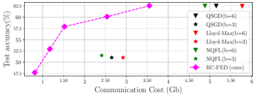
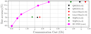
We evaluate RC-FED through some numerical experiments and compare it against the state-of-the-art. As baseline we consider traditional QSGD [8], Lloyd-Max quantizer [16], and NQFL [14]. We test the benchmark schemes for . For a fair comparison, we use Huffman coding to compress the quantized gradients in all methods. We compute the test accuracy of the trained models and sketch them against the communication costs required for the entire training.
We first consider CIFAR-10 with similar setups to those in [21, 22]. We distribute the dataset among clients using Dirichlet allocation with and train ResNet-18 for 100 communication rounds with single local iterations. The batch size is set to 64 and .
We next consider the federated extended MNIST (FEMNIST) dataset, which is a federated image classification dataset distributed over 3550 devices with 62 classes [23]. We train a classic CNN with two convolutional layers followed by two fully-connected layers. The batch size is 32. At each round, devices are randomly sampled out of the 3550 ones and locally train for local iterations using the default data stored in each device.
Performance Comparison
The results for CIFAR-10 and FEMNIST datasets are depicted in Figs. 1a and 1b, respectively. For RC-FED, we plot the results for various resulting in a curve. As observed, for the same test accuracy, RC-FED requires significantly lower communication costs. For instance, considering CIFAR-10 dataset, RC-FED achieves and test accuracy with 3.55 Gigabits (Gb) and 1.17 Gb of data transmission, which is significantly lower than that required by the benchmarks. This empirically validate the effectiveness of quantization with rate constraint.
6 Conclusion
This paper introduced RC-FED, a quantized FL framework in which clients quantize their local gradients by simultaneously minimizing distortion and restricting the data rate achieved after encoding the quantized gradients. Numerical results showed that RC-FED () significantly reduces the communication overhead as compared with baselines, while maintaining the test accuracy, and () establishes a tunable trade-off between communication overhead and test accuracy. A natural direction for future work is to extend the RC-FED framework beyond scalar quantization.
References
- [1] B. McMahan, E. Moore, D. Ramage, S. Hampson, and B. A. Arcas, “Communication-efficient learning of networks from decentralized data,” in Artificial intelligence and statistics. PMLR, 2017.
- [2] J. Park, S. Samarakoon, A. Elgabli, J. Kim, M. Bennis, S.-L. Kim, and M. Debbah, “Communication-efficient and distributed learning over wireless networks: Principles and applications,” Proceedings of the IEEE, vol. 109, no. 5, pp. 796–819, 2021.
- [3] S. M. Hamidi, M. Mehrabi, A. K. Khandani, and D. Gündüz, “Over-the-air federated learning exploiting channel perturbation,” in Proc. IEEE (SPAWC), 2022.
- [4] S. M. Hamidi, “Training neural networks on remote edge devices for unseen class classification,” IEEE Signal Processing Letters, vol. 31, pp. 1004–1008, 2024.
- [5] S. M. Hamidi, R. Tan, L. Ye, and E.-H. Yang, “Fed-IT: Addressing class imbalance in federated learning through an information-theoretic lens,” in Proc. IEEE (ISIT), 2024.
- [6] A. Z. Tan, H. Yu, L. Cui, and Q. Yang, “Towards personalized federated learning,” IEEE Trans. Neural Netw. Learn. Syst., vol. 34, no. 12, pp. 9587–9603, 2023.
- [7] M. M. Amiri, D. Gunduz, S. R. Kulkarni, and H. V. Poor, “Federated learning with quantized global model updates,” arXiv preprint arXiv:2006.10672, 2020.
- [8] D. Alistarh, D. Grubic, J. Li, R. Tomioka, and M. Vojnovic, “Qsgd: Communication-efficient sgd via gradient quantization and encoding,” Advances in neural information processing systems, vol. 30, 2017.
- [9] S. U. Stich, J.-B. Cordonnier, and M. Jaggi, “Sparsified sgd with memory,” Advances in neural information processing systems, vol. 31, 2018.
- [10] Y. Jiang, S. Wang, V. Valls, B. J. Ko, W.-H. Lee, K. K. Leung, and L. Tassiulas, “Model pruning enables efficient federated learning on edge devices,” IEEE Trans. Neural Netw. Learn. Syst., vol. 34, no. 12, pp. 10 374–10 386, 2022.
- [11] N. Shlezinger, M. Chen, Y. C. Eldar, H. V. Poor, and S. Cui, “Uveqfed: Universal vector quantization for federated learning,” IEEE Trans. Signal Process., vol. 69, pp. 500–514, 2021.
- [12] A. Elgabli, J. Park, A. S. Bedi, C. B. Issaid, M. Bennis, and V. Aggarwal, “Q-gadmm: Quantized group admm for communication efficient decentralized machine learning,” IEEE Trans. Commun., vol. 69, no. 1, pp. 164–181, 2020.
- [13] S. Chen, C. Shen, L. Zhang, and Y. Tang, “Dynamic aggregation for heterogeneous quantization in federated learning,” IEEE Trans. Wirel. Commun., vol. 20, no. 10, pp. 6804–6819, 2021.
- [14] G. Chen, K. Xie, Y. Tu, T. Song, Y. Xu, J. Hu, and L. Xin, “Nqfl: Nonuniform quantization for communication efficient federated learning,” IEEE Commun. Letters, 2023.
- [15] N. Shlezinger, M. Chen, Y. C. Eldar, H. V. Poor, and S. Cui, “Federated learning with quantization constraints,” in Proc. IEEE (ICASSP), 2020.
- [16] L. Chen, W. Liu, Y. Chen, and W. Wang, “Communication-efficient design for quantized decentralized federated learning,” IEEE Trans. Signal Process., 2024.
- [17] N. Zhang, M. Tao, J. Wang, and F. Xu, “Fundamental limits of communication efficiency for model aggregation in distributed learning: A rate-distortion approach,” IEEE Trans. on Comm., vol. 71, no. 1, pp. 173–186, 2022.
- [18] J. Lee, Y. Bahri, R. Novak, S. S. Schoenholz, J. Pennington, and J. Sohl-Dickstein, “Deep neural networks as gaussian processes,” in International Conference on Learning Representations, 2018.
- [19] S. Lloyd, “Least squares quantization in pcm,” IEEE Trans. Inf. Theory, vol. 28, no. 2, pp. 129–137, 1982.
- [20] X. Li, K. Huang, W. Yang, S. Wang, and Z. Zhang, “On the convergence of fedavg on non-iid data,” in International Conference on Learning Representations, 2019.
- [21] S. M. Hamidi and E.-H. YANG, “Adafed: Fair federated learning via adaptive common descent direction,” Transactions on Machine Learning Research, 2024.
- [22] S. Mohajer Hamidi and O. Damen, “Fair wireless federated learning through the identification of a common descent direction,” IEEE Commun. Letters, vol. 28, no. 3, pp. 567–571, 2024.
- [23] S. Caldas, S. M. K. Duddu, P. Wu, T. Li, J. Konečnỳ, H. B. McMahan, V. Smith, and A. Talwalkar, “Leaf: A benchmark for federated settings,” arXiv preprint arXiv:1812.01097, 2018.
- [24] P. Panter and W. Dite, “Quantization distortion in pulse-count modulation with nonuniform spacing of levels,” Proceedings of the IRE, vol. 39, no. 1, pp. 44–48, 1951.
7 Proof of Theorem 1
If A(III) and A(IV) hold, and , then based on [20] (see Lemma 1 therein), we have
| (13) |
where is the updated model parameter at client . To bound and in (13), we introduce Lemmas 1 and 2 whose proofs are provided in supporting documents:
Lemma 1.
Assume that assumption A(I) holds, and that local clients perform local epochs of training, then
| (14) |
Lemma 2.
Assume that the gradient distribution for client follows Gaussian distribution with standard deviation , and that the clients use for gradient quantization, then
| (15) |
Using Lemmas 1 and 2 in (13), we obtain
| (16) |
which is a recursive expression. The theorem can be concluded by using A(III) and induction over in (16) (the full proof is analogous to the proof of Theorem 1 in [20]).
7.1 Proof of Lemma 1
Since the clients perform local epochs, there exists such that , and , . Also, note that is non-increasing, and . Then, we have
| (17) |
which concludes Lemma 1.
7.2 Proof of Lemma 2
Here, entropy and differential entropy are denoted by and , respectively.
First note that using Lloyd quantizers, the MSE distortion becomes [24].
Assume a high-rate scenario, where is large enough. Then, the PDF is almost constant in each quantization interval. As such, , and thus . Hence, the rate could be obtained as follows
| (18) | ||||
| (19) |
where in (18), denotes the differentiable entropy, and we used Jensen’s inequality to derived the inequality in (18). From (19), it is concluded that
| (20) |
For , the expression in (20) is simplified to
| (21) |
Knowing that , then we have
| (22) |
which concludes the Lemma 2.