First Radial Excitations of Baryons in a Contact Interaction: Mass Spectrum

Abstract

We compute masses of twenty positive parity first radial excitations of spin-$1/2$ and $3/2$ baryons composed of ${\color[rgb]{1,0,0}u}$, ${\color[rgb]{0.64,0.0,0.0}d}$, ${\color[rgb]{0,0.5,0}s}$, ${\color[rgb]{0.55,0.0,0.55}c}$ and ${\color[rgb]{0,0,1}b}$ quarks in a quark-diquark picture within a contact interaction model. These excitations comprise of two elements: one characterized by a zero in the Faddeev amplitude, representing a radial excitation of the quark-diquark system and the other marked by a zero in the diquark’s Bethe-Salpeter amplitude, corresponding to an intrinsic excitation of the diquark correlation. Wherever possible, we compare our results with other models and/or experiment. We verify that the masses obtained through our model conform to the spacing rules for all the baryons studied, whether light or heavy and whether of spin 1/2 or 3/2. The computed masses do not just offer a guide to the future experimental searches but also compare well with the existing candidates for the possible radial excitations of some heavy baryons.

I Introduction

More than sixty years ago, the Faddeev equation was first proposed in Ref. Faddeev (1960) to investigate the three-body bound states. Therefore, this equation is ideally suited to study baryons. However, this problem can be reduced to two-body subsystems if we employ a quark-diquark picture. It is well-known by now that the difference between these two approaches yields a difference between the computed baryon masses of merely about 5%, see Refs. Eichmann (2011); Eichmann et al. (2016). The obvious advantage is that it considerably reduces mathematical and computational difficulties by converting a three-body problem into a two-body one. Gell-Mann suggested the idea of diquarks in his renowned article of 1964 Gell-Mann (1964). Within a couple of years, some of the earliest attempts to compute baryon masses were made in Refs. Ida and Kobayashi (1966); Lichtenberg and Tassie (1967). Static point-like diquarks were used in efforts to explain the problem of missing resonances as early as in 1969 Lichtenberg (1969).

The diquarks that we employ in our work are dynamical in nature with finite electromagnetic extent and an associated mass-scale which are both bounded below by the corresponding quantities characterizing the analogous mesonic system. A comprehensive review, Ref. Barabanov et al. (2021), and the references therein, are an excellent source on our improved understanding of diquarks and the role they play in studying the baryon spectrum and their internal structure. Diquarks are paired color non-singlet correlations of two quarks. Owing to their color charge, these correlations are confined within baryons, tetra-quarks or penta-quarks, making direct observation impossible. Two quarks can form product representation in a color sextet or an antitriplet configuration. When exchanging a single gluon, a simple analysis of color flow indicates that attractive interaction occurs between diquarks in a color antitriplet arrangement while it is repulsive for a sextet. Moreover, the diquark in a color antitriplet state can bind with a quark to create a color-singlet baryon. That is why these are dubbed as good diquarks Wilczek (2004). Therefore, we shall exclusively focus on $qq$ states in a color antitriplet configuration. Similarly to mesons, various types of diquarks are distinguished by distinct Dirac structures. Therefore, we have scalar, pseudo-scalar, vector and axial-vector diquarks.

One expects dozens of baryonic states with singly, doubly, and triply heavy quarks. Studying radially excited baryons is naturally more complex than studying their counterpart ground states. Identification and analysis of these states is equally challenging in the experiments. Radial excitations of baryons with two heavy quarks have been thoroughly studied through Poincaré-covariant Faddeev equation (FE) for baryons Qin et al. (2019) (we refer to this model as QRS, after the initials of the authors of the Ref. Qin et al. (2019)), relativistic quark model Ebert et al. (2002), quark model Yoshida et al. (2015), Salpeter model Giannuzzi (2009), hypercentral constituent quark model Shah and Rai (2017a); Shah et al. (2016), the heavy quark effective theory (HQET) Vishwakarma and Upadhyay (2022), Faddeev method Valcarce et al. (2008), QCD sum rules Shekari Tousi and Azizi (2024); Alrebdi et al. (2022); Alomayrah and Barakat (2020) and Regge phenomenology Oudichhya et al. (2021); Shah and Rai (2017b). These baryons are significant as they represent potential candidates for the states recently observed by the LHCb experiment. For example, initial observations of the baryon $\Omega_{{\color[rgb]{0,0,1}b}}^{-}$ with a mass of approximately 6.35 GeV suggest that this state corresponds to the first radial excitation of $\Omega_{{\color[rgb]{0,0,1}b}}^{-}({\color[rgb]{0,0.5,0}s}{\color[rgb]{0,0.5,0}s}{\color[rgb]{0,0,1}b})$ Aaij et al. (2020). The LHCb collaboration reported the observation of $\Xi_{{\color[rgb]{0,0,1}b}}^{-}$ with mass 6.226 GeV. From the observed mass and decay modes, it was suggested that $\Xi_{{\color[rgb]{0,0,1}b}}^{-}$ state might be $1P$ or $2S$ excited baryon Aaij et al. (2018); Aliev et al. (2018). LHCb has also detected two excited $\Omega_{{\color[rgb]{0.55,0.0,0.55}c}}$ states decaying to $\Xi_{{\color[rgb]{0.55,0.0,0.55}c}}K^{-}$ with masses of around 3.18 GeV and 3.3 GeV and which can be interpreted as radial excitations of $\Omega_{{\color[rgb]{0.55,0.0,0.55}c}}^{0}({\color[rgb]{0,0.5,0}s}{\color[rgb]{0,0.5,0}s}{\color[rgb]{0.55,0.0,0.55}c})$ and $\Omega_{{\color[rgb]{0.55,0.0,0.55}c}}^{0*}{({\color[rgb]{0,0.5,0}s}{\color[rgb]{0,0.5,0}s}{\color[rgb]{0.55,0.0,0.55}c})}$, respectively Karliner and Rosner (2023); Aaij et al. (2023); Pan and Pan (2024). Contact interaction (CI) is a useful theoretical tool to explore the static properties of hadrons, particularly their masses. In Ref. Paredes-Torres et al. (2024), masses of radial excitations of mesons and diquarks were computed using this model. We extend that work to investigate baryons and compute the masses of their first radial excitations in the light and heavy sectors. For that purpose, we have organized this paper as follows: in Section II, a comprehensive examination of the FE for baryons with different spins is conducted; Section III is dedicated to elucidate the essential ingredients of our model to compute radial excitations rather accurately; Our results, along with the corresponding analysis, are detailed in Section IV; and finally, a summary and outlook is presented in Section V.

II Faddeev Equation

We base our description of baryons-bound states in the quark-diquark approximation on FE, which is illustrated in Fig. 1.

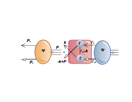
Figure 1: Poincaré covariant FE employed in this work to calculate masses of the first radial excitation of baryons. The red square represents the quark-diquark interaction Kernel. The single line denotes the dressed quark, the double line is the diquark while $\Gamma$ and $\Psi$ are the Bethe-Salpeter and Faddeev amplitudes (BSA and FA) , respectively. Configuration of momenta is: $\ell_{qq}=-\ell+P$, $k_{qq}=-k+P$, $P=P_{d}+P_{q}$.

In this section, we shall examine this FE in detail and the requisite components for our computation, adhering closely to the notation employed in Ref. Gutiérrez-Guerrero et al. (2019). Using this equation, we can predict the masses of ground and radially excited baryons with $J^{P}=1/2^{+}$ and $J^{P}=3/2^{+}$, where $J$ is the total spin and $P$ denotes the parity.
Fig. 2 presents the $SU(5)$ flavor depiction of these states. The baryons multiplets that arise from $3\otimes 3\otimes 3$ are: a decouplet, two octets and a singlet. The corresponding multiplet structure for $SU(4)$ is $4\otimes 4\otimes 4=20_{S}\oplus 20_{MS}\oplus 20_{MA}\oplus 4_{A}$. Note that explicit quark masses break the flavor symmetry. The larger the group, the more significant the amount of breaking as each new quark is significantly heavier. However, this group algebra approach helps us identify the baryons whose masses we are interested to compute. As only a representative example, we present such baryon multiplets with ${\color[rgb]{1,0,0}u}$, ${\color[rgb]{0.64,0.0,0.0}d}$, ${\color[rgb]{0,0.5,0}s}$ and ${\color[rgb]{0,0,1}b}$ quark in Fig. 2. The multiplet with charm quarks is analogous to the one containing the bottom quark. A detailed examination of the FE delineating states both with $J=1/2$ and $J=3/2$ will be undertaken in the ensuing subsections.

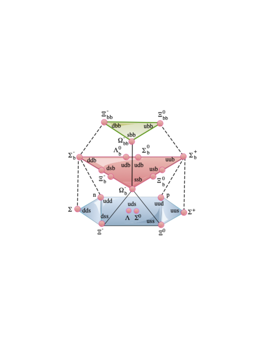
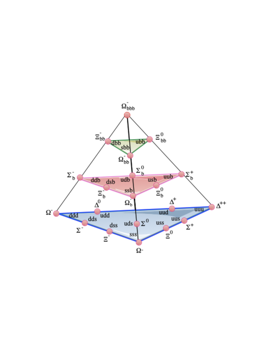
Figure 2: Left: Baryons with spin $1/2$.- We show the mixed-symmetric $20$-plet. Note that all the ground-state baryons in this multiplet have $J^{P}=(1/2)^{+}$. It has the $SU(3)$ octet on the lowest layer. The singly heavy baryons are composed of a bottom quark and two light quarks $({\color[rgb]{1,0,0}u},{\color[rgb]{0.64,0.0,0.0}d},{\color[rgb]{0,0.5,0}s})$, located in the second layer. The doubly heavy baryons are positioned in the top-most layer. Right: Baryons with spin $3/2$.- It depicts states of baryons with spin $3/2$ made from four quarks of the types ${\color[rgb]{1,0,0}u},{\color[rgb]{0.64,0.0,0.0}d},{\color[rgb]{0,0.5,0}s}$, and ${\color[rgb]{0,0,1}b}$. Doubly heavy baryons and triply heavy baryons are localized in the highest layers.

II.1 Baryons with spin 1/2

The mass of the ground-state baryon with spin $1/2$ comprised by the quarks $[{\color[rgb]{1,0,0}q}{\color[rgb]{1,0,0}q}{\color[rgb]{0,0,1}q_{1}}]$ and the momentum configuration given in Fig. 1 is determined by a $5\times 5$ matrix FE. It can be written in the following form :

$$\left[\begin{array}[]{r}{\cal S}(k;P)\,u(P)\\ {\cal A}^{i}_{\mu}(k;P)\,u(P)\end{array}\right]$$ (3)

$$= -\,4\,\int\frac{d^{4}\ell}{(2\pi)^{4}}\,{\cal M}(k,\ell;P)\left[\begin{array}[]{r}{\cal S}(\ell;P)\,u(P)\\ {\cal A}^{j}_{\nu}(\ell;P)\,u(P)\end{array}\right].\rule{10.00002pt}{0.0pt}$$ (6)

The general matrices ${\cal S}(\ell;P)$ and ${\cal A}^{i}_{\nu}(\ell;P)$, which describe the momentum-space correlation between a quark and a diquark in the nucleon and the roper are described in Refs. Oettel et al. (1998); Cloet et al. (2007). However, with the CI employed in this article, they simplify considerably :

$${\cal S}(P) = s(P)\,\mbox{\boldmath$I$}_{\rm D}\,,$$ (7a)

$${\cal A}^{i}_{\mu}(P) = a_{1}^{i}(P)\gamma_{5}\gamma_{\mu}+a_{2}^{i}(P)\gamma_{5}\hat{P}_{\mu}\,,\quad i=+,0\rule{20.00003pt}{0.0pt}$$ (7b)

where the scalars $s$ and $a_{1,2}^{i}$ are independent of the relative quark-diquark momentum and $\hat{P}^{2}=-1$. FA is thus represented by the eigenvector :

$$\Psi(P)=\left[\begin{array}[]{c}s(P)\\[3.01385pt] a_{1}^{+}(P)\\[3.01385pt] a_{1}^{0}(P)\\[3.01385pt] a_{2}^{+}(P)\\[3.01385pt] a_{2}^{0}(P)\end{array}\right]\,.$$ (8)

The Kernel in Eq. (6) can generically be expanded as

$${\cal M}(k,\ell;P)=\begin{pmatrix}\mathcal{M}^{11}&\mathcal{M}^{12}_{\nu}&\mathcal{M}^{13}_{\nu}&\mathcal{M}^{14}_{\nu}&\mathcal{M}^{15}_{\nu}\\ \\ \mathcal{M}^{21}_{\mu}&\mathcal{M}^{22}_{\mu\nu}&\mathcal{M}^{23}_{\mu\nu}&\mathcal{M}^{24}_{\mu\nu}&\mathcal{M}^{25}_{\mu\nu}\\ \\ \mathcal{M}^{31}_{\mu}&\mathcal{M}^{32}_{\mu\nu}&\mathcal{M}^{33}_{\mu\nu}&\mathcal{M}^{34}_{\mu\nu}&\mathcal{M}^{35}_{\mu\nu}\\ \\ \mathcal{M}^{41}_{\mu}&\mathcal{M}^{42}_{\mu\nu}&\mathcal{M}^{43}_{\mu\nu}&\mathcal{M}^{44}_{\mu\nu}&\mathcal{M}^{45}_{\mu\nu}\\ \\ \mathcal{M}^{51}_{\mu}&\mathcal{M}^{52}_{\mu\nu}&\mathcal{M}^{53}_{\mu\nu}&\mathcal{M}^{54}_{\mu\nu}&\mathcal{M}^{55}_{\mu\nu}\\ \end{pmatrix}\,.$$ (9)

The elements of the matrix in Eq. (LABEL:B-matrix) are detailed in Appendix D. In order to simplify Eqs. (6), we use static approximation for the exchanged quark with mass $M$ and flavor $f$. It was introduced first in Ref. Buck et al. (1992) :

$$S(p)=\frac{1}{i\gamma\cdot p+M_{f}}\to\frac{1}{M_{f}}\,.$$ (10)

A variation of it was implemented in Ref. Xu et al. (2015),

$$S(p)=\frac{1}{i\gamma\cdot p+M_{f}}\to\frac{g_{B}}{i\gamma\cdot p+M_{f}}\,.$$ (11)

We follow Refs. Roberts et al. (2011a); Lu et al. (2017); Chen et al. (2012) and represent the quark (propagator) exchanged between the diquarks as

$$S^{\rm T}(k)\to\frac{g_{B}}{M_{f}}\,.$$ (12)

The superscript “T” indicates matrix transpose. However, in the implementation of this framework to heavy baryons in the ground state with spin $1/2$, it suffices to use $g_{B}=1$, as discussed in reference Gutiérrez-Guerrero et al. (2019). For radial excitations, however, this value will no longer be $1$, as will be explained in the subsequent sections.
The spin-$1/2$ heavy baryons are represented by the following column matrices:

$$\begin{array}[]{cc}u_{\Xi_{cc}^{++}({\color[rgb]{1,0,0}u}{\color[rgb]{0.55,0.0,0.55}c}{\color[rgb]{0.55,0.0,0.55}c})}=\left[\begin{array}[]{c}[{\color[rgb]{1,0,0}u}{\color[rgb]{0.55,0.0,0.55}c}]{\color[rgb]{0.55,0.0,0.55}c}\\ \{{\color[rgb]{0.55,0.0,0.55}c}{\color[rgb]{0.55,0.0,0.55}c}\}{\color[rgb]{1,0,0}u}\\ \{{\color[rgb]{1,0,0}u}{\color[rgb]{0.55,0.0,0.55}c}\}{\color[rgb]{0.55,0.0,0.55}c}\\ \end{array}\right],&u_{\Omega_{{\color[rgb]{0.55,0.0,0.55}c}{\color[rgb]{0.55,0.0,0.55}c}}^{+}({\color[rgb]{0,0.5,0}s}{\color[rgb]{0.55,0.0,0.55}c}{\color[rgb]{0.55,0.0,0.55}c})}=\left[\begin{array}[]{c}[{\color[rgb]{0,0.5,0}s}{\color[rgb]{0.55,0.0,0.55}c}]{\color[rgb]{0.55,0.0,0.55}c}\\ \{{\color[rgb]{0.55,0.0,0.55}c}{\color[rgb]{0.55,0.0,0.55}c}\}{\color[rgb]{0,0.5,0}s}\\ \{{\color[rgb]{0,0.5,0}s}{\color[rgb]{0.55,0.0,0.55}c}\}{\color[rgb]{0.55,0.0,0.55}c}\\ \end{array}\right],\end{array}$$

$$\begin{array}[]{cc}u_{\Omega_{{\color[rgb]{0.55,0.0,0.55}c}}^{0}({\color[rgb]{0,0.5,0}s}{\color[rgb]{0,0.5,0}s}{\color[rgb]{0.55,0.0,0.55}c})}=\left[\begin{array}[]{c}[{\color[rgb]{0,0.5,0}s}{\color[rgb]{0.55,0.0,0.55}c}]{\color[rgb]{0,0.5,0}s}\\ \{{\color[rgb]{0,0.5,0}s}{\color[rgb]{0,0.5,0}s}\}{\color[rgb]{0.55,0.0,0.55}c}\\ \{{\color[rgb]{0,0.5,0}s}{\color[rgb]{0.55,0.0,0.55}c}\}{\color[rgb]{0,0.5,0}s}\\ \end{array}\right],&u_{\Sigma_{{\color[rgb]{0.55,0.0,0.55}c}}^{++}({\color[rgb]{1,0,0}u}{\color[rgb]{1,0,0}u}{\color[rgb]{0.55,0.0,0.55}c})}=\left[\begin{array}[]{c}[{\color[rgb]{1,0,0}u}{\color[rgb]{0.55,0.0,0.55}c}]{\color[rgb]{1,0,0}u}\\ \{{\color[rgb]{1,0,0}u}{\color[rgb]{1,0,0}u}\}{\color[rgb]{0.55,0.0,0.55}c}\\ \{{\color[rgb]{1,0,0}u}{\color[rgb]{0.55,0.0,0.55}c}\}{\color[rgb]{1,0,0}u}\\ \end{array}\right],\end{array}$$

$$\begin{array}[]{cc}u_{\Xi_{bb}^{0}({\color[rgb]{1,0,0}u}{\color[rgb]{0,0,1}b}{\color[rgb]{0,0,1}b})}=\left[\begin{array}[]{c}[{\color[rgb]{1,0,0}u}{\color[rgb]{0,0,1}b}]{\color[rgb]{0,0,1}b}\\ \{{\color[rgb]{0,0,1}b}{\color[rgb]{0,0,1}b}\}{\color[rgb]{1,0,0}u}\\ \{{\color[rgb]{1,0,0}u}{\color[rgb]{0,0,1}b}\}{\color[rgb]{0,0,1}b}\\ \end{array}\right],&u_{\Omega_{bb}^{-}({\color[rgb]{0,0.5,0}s}{\color[rgb]{0,0,1}b}{\color[rgb]{0,0,1}b})}=\left[\begin{array}[]{c}[{\color[rgb]{0,0.5,0}s}{\color[rgb]{0,0,1}b}]{\color[rgb]{0,0,1}b}\\ \{{\color[rgb]{0,0,1}b}{\color[rgb]{0,0,1}b}\}{\color[rgb]{0,0.5,0}s}\\ \{{\color[rgb]{0,0.5,0}s}{\color[rgb]{0,0,1}b}\}{\color[rgb]{0,0,1}b}\\ \end{array}\right],\end{array}$$

$$\begin{array}[]{cc}u_{\Omega_{b}^{-}({\color[rgb]{0,0.5,0}s}{\color[rgb]{0,0.5,0}s}{\color[rgb]{0,0,1}b})}=\left[\begin{array}[]{c}[{\color[rgb]{0,0.5,0}s}{\color[rgb]{0,0,1}b}]{\color[rgb]{0,0.5,0}s}\\ \{{\color[rgb]{0,0.5,0}s}{\color[rgb]{0,0.5,0}s}\}{\color[rgb]{0,0,1}b}\\ \{{\color[rgb]{0,0.5,0}s}{\color[rgb]{0,0,1}b}\}{\color[rgb]{0,0.5,0}s}\\ \end{array}\right],&u_{\Sigma_{b}^{+}({\color[rgb]{1,0,0}u}{\color[rgb]{1,0,0}u}{\color[rgb]{0,0,1}b})}=\left[\begin{array}[]{c}[{\color[rgb]{1,0,0}u}{\color[rgb]{0,0,1}b}]{\color[rgb]{1,0,0}u}\\ \{{\color[rgb]{1,0,0}u}{\color[rgb]{1,0,0}u}\}{\color[rgb]{0,0,1}b}\\ \{{\color[rgb]{1,0,0}u}{\color[rgb]{0,0,1}b}\}{\color[rgb]{1,0,0}u}\\ \end{array}\right],\end{array}$$

$$\begin{array}[]{cc}u_{\Omega({\color[rgb]{0.55,0.0,0.55}c}{\color[rgb]{0.55,0.0,0.55}c}{\color[rgb]{0,0,1}b})}=\left[\begin{array}[]{c}[{\color[rgb]{0.55,0.0,0.55}c}{\color[rgb]{0,0,1}b}]{\color[rgb]{0.55,0.0,0.55}c}\\ \{{\color[rgb]{0.55,0.0,0.55}c}{\color[rgb]{0.55,0.0,0.55}c}\}{\color[rgb]{0,0,1}b}\\ \{{\color[rgb]{0.55,0.0,0.55}c}{\color[rgb]{0,0,1}b}\}{\color[rgb]{0.55,0.0,0.55}c}\\ \end{array}\right],&u_{\Omega({\color[rgb]{0.55,0.0,0.55}c}{\color[rgb]{0,0,1}b}{\color[rgb]{0,0,1}b})}=\left[\begin{array}[]{c}[{\color[rgb]{0.55,0.0,0.55}c}{\color[rgb]{0,0,1}b}]{\color[rgb]{0,0,1}b}\\ \{{\color[rgb]{0,0,1}b}{\color[rgb]{0,0,1}b}\}{\color[rgb]{0.55,0.0,0.55}c}\\ \{{\color[rgb]{0.55,0.0,0.55}c}{\color[rgb]{0,0,1}b}\}{\color[rgb]{0,0,1}b}\\ \end{array}\right].\end{array}$$

Note that we use the notation introduced in Ref. Chen et al. (2012), [${\color[rgb]{1,0,0}q}{\color[rgb]{0,0,1}q_{1}}$] for scalar diquarks, and $\{{\color[rgb]{1,0,0}q}{\color[rgb]{1,0,0}q}\},\{{\color[rgb]{1,0,0}q}{\color[rgb]{0,0,1}q_{1}}\}$ for axial-vector diquarks. The Faddeev amplitude for baryons with spin $3/2$ is different from that for spin $1/2$. Below we discuss the fundamentals of the FE and FA of these baryons.

II.2 Baryons with spin-3/2

Baryons with spin-$3/2$ are specially important because they can involve states with three ${\color[rgb]{0.55,0.0,0.55}c}$-quarks and three ${\color[rgb]{0,0,1}b}$-quarks. In order to calculate their masses, we note that it is not possible to combine a spin-zero diquark with a spin-1/2 quark to obtain spin-$3/2$ baryon. Hence, such a baryon is comprised solely of axial-vector correlations. The FA for the positive-energy baryon is :

$$\Psi_{\mu}=\psi_{\mu\nu}(P)u_{\nu}(P)\;,$$

where $P$ is the total momentum of the baryon, $u_{\nu}(P)$ is a Rarita-Schwinger spinor,

$$\psi_{\mu\nu}(P)u_{\nu} = \Gamma_{{\color[rgb]{1,0,0}q}{\color[rgb]{0,0,1}q_{1}},\mu}\Delta_{\mu\nu,_{{\color[rgb]{1,0,0}q}{\color[rgb]{1,0,0}q}}}^{1^{+}}(\ell_{{\color[rgb]{1,0,0}q}{\color[rgb]{1,0,0}q}}){\cal D}_{\nu\rho}(P)u_{\rho}(P)\,,$$ (13)

with $\Delta_{\mu\nu,{\color[rgb]{1,0,0}q}{\color[rgb]{1,0,0}q}}^{1^{+}}$ is the diquark propagator defined in Appendix D and,

$${\cal D}_{\nu\rho}(\ell;P) = {\cal S}(\ell;P)\,\delta_{\nu\rho}+\gamma_{5}{\cal A}_{\nu}(\ell;P)\,\ell^{\perp}_{\rho}\,.$$ (14)

Understanding the structure of these states is simpler than in the case of the nucleon. We have provided more details in Appendix A. In what follows, we only consider the baryons with two possible structures: ${\color[rgb]{1,0,0}q}{\color[rgb]{1,0,0}q}{\color[rgb]{1,0,0}q}$ and ${\color[rgb]{0,0,1}q_{1}}{\color[rgb]{1,0,0}q}{\color[rgb]{1,0,0}q}$.

Baryons (${\color[rgb]{1,0,0}q}{\color[rgb]{1,0,0}q}{\color[rgb]{1,0,0}q}$): Only one possible type of diquarks exists for a baryon composed of same three quarks $({\color[rgb]{1,0,0}q}{\color[rgb]{1,0,0}q}{\color[rgb]{1,0,0}q})$. In this case, the FA is:

$${\cal D}_{\nu\rho}(\ell;P)u_{\rho}^{B}(P)=f^{B}(P)\,\mathbf{I}_{\rm D}\,u_{\nu}^{B}(P)\,.$$ (15)

Employing Feynman rules for Fig. 1 and using the expression for the FA, Eq. (15), we can write

$$f^{B}(P)u_{\mu}^{B}(P)=4\frac{g_{B}}{M_{{\color[rgb]{1,0,0}q}}}\int\frac{d^{4}\ell}{(2\pi)^{4}}\mathcal{M_{\mu\nu}}f^{B}(P)u_{\nu}^{B}(P)\,,$$ (16)

where we have suppressed the functional dependence of $\mathcal{M}_{\mu\nu}$ on momenta for simplicity, and

$$\mathcal{M}_{\mu\nu} = 2i{\color[rgb]{0,0,0}\Gamma}^{1^{+}}_{\{{\color[rgb]{1,0,0}q}{\color[rgb]{1,0,0}q}\},\rho}(l_{{\color[rgb]{1,0,0}q}{\color[rgb]{1,0,0}q}})i\overline{{\color[rgb]{0,0,0}\Gamma}}^{1^{+}}_{\{{\color[rgb]{1,0,0}q}{\color[rgb]{1,0,0}q}\},\mu}(-k_{{\color[rgb]{1,0,0}q}{\color[rgb]{1,0,0}q}})S_{{\color[rgb]{0,0,1}q_{1}}}(l_{{\color[rgb]{0,0,1}q_{1}}}){\color[rgb]{0,0,0}\Delta}^{1^{+}}_{\{{\color[rgb]{1,0,0}q}{\color[rgb]{1,0,0}q}\},\rho\nu}(l_{{\color[rgb]{1,0,0}q}{\color[rgb]{1,0,0}q}})\;.$$

We now multiply both sides by ${\bar{u}}^{B}_{\beta}(P)$ from the left and sum over the polarization not explicitly shown here, to obtain

$$\Lambda_{+}(P)R_{\mu\beta}(P)=4\frac{g_{B}}{M_{{\color[rgb]{1,0,0}q}}}\int\frac{d^{4}\ell}{(2\pi)^{4}}\mathcal{M_{\mu\nu}}\Lambda_{+}(P)R_{\nu\beta}\,.$$ (17)

Positive energy projection operator $\Lambda_{+}$ and $R_{\mu\beta}$ are defined in Eqs. (A.7) and (A.14) in Appendix A. Finally we contract with $\delta_{\mu\beta}$ and with the aid of a Feynman parametrisation, we obtain

$$2\pi^{2}=\frac{g_{B}}{M_{{\color[rgb]{1,0,0}q}}}\frac{E_{\{{\color[rgb]{1,0,0}q}{\color[rgb]{1,0,0}q}\}_{1^{+}}}^{2}}{m_{\{{\color[rgb]{1,0,0}q}{\color[rgb]{1,0,0}q}\}_{1^{+}}}^{2}}\int_{0}^{1}d\alpha\,{\cal L}^{\Omega}\overline{\cal C}^{\rm iu}_{1}(\omega(\alpha,M_{{\color[rgb]{1,0,0}q}}^{2},m^{2}_{\{{\color[rgb]{1,0,0}q}{\color[rgb]{1,0,0}q}\}_{1^{+}}},P^{2}))\,,$$

(18)

where $E_{\{{\color[rgb]{1,0,0}q}{\color[rgb]{1,0,0}q}\}_{1^{+}}}$ is the structure in the BSA in Eq. (C) in Appendix C. The function ${\cal C}^{\rm iu}_{1}$ is defined in Eq. (B.20) in the Appendix  B, and $m_{\{{\color[rgb]{1,0,0}q}{\color[rgb]{1,0,0}q}\}_{1^{+}}}$ is de diquark mass. We have defined

$${\cal L}^{\Omega} = [m_{\{{\color[rgb]{1,0,0}q}{\color[rgb]{1,0,0}q}\}_{1^{+}}}^{2}-(1-\alpha)^{2}P^{2}][-\alpha P^{2}+M_{{\color[rgb]{1,0,0}q}}]\,,$$

$$\omega(\alpha,M_{{\color[rgb]{1,0,0}q}}^{2},m^{2}_{\{{\color[rgb]{1,0,0}q}{\color[rgb]{1,0,0}q}\}_{1^{+}}},P^{2}) = M_{{\color[rgb]{1,0,0}q}}^{2}(1-\alpha)+\alpha m^{2}_{\{{\color[rgb]{1,0,0}q}{\color[rgb]{1,0,0}q}\}_{1^{+}}}$$

$$+ \alpha(1-\alpha)P^{2}\,,$$

The color-singlet bound states constructed from three identical heavy charm/bottom quarks are:

$$\begin{array}[]{cc}u_{\Omega_{{\color[rgb]{0.55,0.0,0.55}c}{\color[rgb]{0.55,0.0,0.55}c}{\color[rgb]{0.55,0.0,0.55}c}}^{++*}}=\left[\begin{array}[]{c}\{{\color[rgb]{0.55,0.0,0.55}c}{\color[rgb]{0.55,0.0,0.55}c}\}{\color[rgb]{0.55,0.0,0.55}c}\\ \end{array}\right],&\hskip 28.45274ptu_{\Omega_{{\color[rgb]{0,0,1}b}{\color[rgb]{0,0,1}b}{\color[rgb]{0,0,1}b}}^{-*}}=\left[\begin{array}[]{c}\{{\color[rgb]{0,0,1}b}{\color[rgb]{0,0,1}b}\}{\color[rgb]{0,0,1}b}\\ \end{array}\right],\end{array}$$ (22)

From the Eq. (18), it is straightforward to compute the mass of these baryons.

Baryons(${\color[rgb]{0,0,1}q_{1}}{\color[rgb]{1,0,0}q}{\color[rgb]{1,0,0}q}$): For a baryon with the quark component structure (${\color[rgb]{0,0,1}q_{1}}{\color[rgb]{1,0,0}q}{\color[rgb]{1,0,0}q}$), there are two possible diquarks, $\{{\color[rgb]{1,0,0}q}{\color[rgb]{1,0,0}q}\}$ and $\{{\color[rgb]{0,0,1}q_{1}}{\color[rgb]{1,0,0}q}\}$. The FA for such a baryon is:

$${\cal D}_{\nu\mu}^{B}(P)u_{\mu}^{B}(P;s)=\sum_{i=\{{\color[rgb]{0,0,1}q_{1}}{\color[rgb]{1,0,0}q}\},\{{\color[rgb]{1,0,0}q}{\color[rgb]{1,0,0}q}\}}d^{i}(P)\delta_{\nu\lambda}u_{\lambda}^{B}(P;s),$$ (23)

so that the corresponding FE has the form

$$\left[\begin{matrix}d^{\{{\color[rgb]{0,0,1}q_{1}}{\color[rgb]{1,0,0}q}\}}\\ d^{\{{\color[rgb]{1,0,0}q}{\color[rgb]{1,0,0}q}\}}\end{matrix}\right]u_{\mu}^{B}=-4\int\frac{d^{4}l}{(2\pi)^{4}}\\ {\cal M}\left[\begin{matrix}d^{\{{\color[rgb]{0,0,1}q_{1}}{\color[rgb]{1,0,0}q}\}}\\ d^{\{{\color[rgb]{1,0,0}q}{\color[rgb]{1,0,0}q}\}}\end{matrix}\right]u_{\nu}^{B}\,,$$ (24)

where

$$\cal{M}=\left[\begin{matrix}{\cal M}_{\mu\nu}^{11}&{\cal M}_{\mu\nu}^{12}\\ \rule{0.0pt}{15.0694pt}{\cal M}_{\mu\nu}^{21}&{\cal M}_{\mu\nu}^{22}\end{matrix}\right]\;,$$ (25)

with the elements of the matrix ${\cal M}$ given by :

$$\begin{split}{\cal M}_{\mu\nu}^{11}&=t^{f_{11}}\frac{{\color[rgb]{1,0,0}g_{B}}}{M_{{\color[rgb]{0,0,1}q_{1}}}}\,\Gamma_{\rho}^{1^{+}}(\ell_{{\color[rgb]{0,0,1}q_{1}}{\color[rgb]{1,0,0}q}})\,\bar{\Gamma}_{\mu}^{1^{+}}(-k_{{\color[rgb]{0,0,1}q_{1}}{\color[rgb]{1,0,0}q}})\,S(l_{{\color[rgb]{1,0,0}q}})\,\Delta_{\rho\nu}^{1^{+}}(\ell_{{\color[rgb]{0,0,1}q_{1}}{\color[rgb]{1,0,0}q}}),\\ {\cal M}_{\mu\nu}^{12}&=t^{f_{12}}\frac{{\color[rgb]{1,0,0}g_{B}}}{M_{{\color[rgb]{1,0,0}q}}}\,\Gamma_{\rho}^{1^{+}}(\ell_{{\color[rgb]{1,0,0}q}{\color[rgb]{1,0,0}q}})\,\bar{\Gamma}_{\mu}^{1^{+}}(-k_{{\color[rgb]{0,0,1}q_{1}}{\color[rgb]{1,0,0}q}})\,S(l_{q_{1}})\,\Delta_{\rho\nu,\{{\color[rgb]{1,0,0}q}{\color[rgb]{1,0,0}q}\}}^{1^{+}}(\ell_{{\color[rgb]{1,0,0}q}{\color[rgb]{1,0,0}q}}),\\ {\cal M}_{\mu\nu}^{21}&=t^{f_{21}}\frac{{\color[rgb]{1,0,0}g_{B}}}{M_{{\color[rgb]{1,0,0}q}}}\,\Gamma_{\rho}^{1^{+}}(\ell_{{\color[rgb]{0,0,1}q_{1}}{\color[rgb]{1,0,0}q}})\,\bar{\Gamma}_{\mu}^{1^{+}}(-k_{{\color[rgb]{1,0,0}q}{\color[rgb]{1,0,0}q}})\,S(l_{{\color[rgb]{1,0,0}q}})\,\Delta_{\rho\nu}^{1^{+}}(\ell_{{\color[rgb]{0,0,1}q_{1}}{\color[rgb]{1,0,0}q}}),\\ {\cal M}_{\mu\nu}^{22}&=t^{f_{22}}\frac{{\color[rgb]{1,0,0}g_{B}}}{M_{{\color[rgb]{1,0,0}q}}}\,\Gamma_{\rho}^{1^{+}}(\ell_{{\color[rgb]{1,0,0}q}{\color[rgb]{1,0,0}q}})\,\bar{\Gamma}_{\mu}^{1^{+}}(-k_{{\color[rgb]{1,0,0}q}{\color[rgb]{1,0,0}q}})\,S(l_{{\color[rgb]{1,0,0}q}_{1}})\,\Delta_{\rho\nu}^{1^{+}}(\ell_{{\color[rgb]{1,0,0}q}{\color[rgb]{1,0,0}q}}),\end{split}$$ (26)

where $t^{f}$ are the flavor matrices and can be found in Appendix E. The color-singlet bound states constructed from three heavy charm/bottom quarks are:

$$\begin{array}[]{cc}u_{\Omega_{{\color[rgb]{0.55,0.0,0.55}c}{\color[rgb]{0.55,0.0,0.55}c}{\color[rgb]{0,0,1}b}}^{+*}}=\left[\begin{array}[]{c}\{{\color[rgb]{0.55,0.0,0.55}c}{\color[rgb]{0.55,0.0,0.55}c}\}{\color[rgb]{0,0,1}b}\\ \{{\color[rgb]{0.55,0.0,0.55}c}{\color[rgb]{0,0,1}b}\}{\color[rgb]{0.55,0.0,0.55}c}\\ \end{array}\right],&\hskip 28.45274ptu_{\Omega_{{\color[rgb]{0.55,0.0,0.55}c}{\color[rgb]{0,0,1}b}{\color[rgb]{0,0,1}b}}^{0*}}=\left[\begin{array}[]{c}\{{\color[rgb]{0.55,0.0,0.55}c}{\color[rgb]{0,0,1}b}\}{\color[rgb]{0,0,1}b}\\ \{{\color[rgb]{0,0,1}b}{\color[rgb]{0,0,1}b}\}{\color[rgb]{0.55,0.0,0.55}c}\end{array}\right].\end{array}$$ (32)

The column vectors representing singly and doubly heavy baryons are:

$$\begin{array}[]{cc}u_{\Sigma_{{\color[rgb]{0.55,0.0,0.55}c}}^{++*}{({\color[rgb]{1,0,0}u}{\color[rgb]{1,0,0}u}{\color[rgb]{0.55,0.0,0.55}c})}}=\left[\begin{array}[]{c}\{{\color[rgb]{1,0,0}u}{\color[rgb]{1,0,0}u}\}{\color[rgb]{0.55,0.0,0.55}c}\\ \{{\color[rgb]{1,0,0}u}{\color[rgb]{0.55,0.0,0.55}c}\}{\color[rgb]{1,0,0}u}\end{array}\right],&\hskip 8.5359ptu_{\Xi_{{\color[rgb]{0.55,0.0,0.55}c}{\color[rgb]{0.55,0.0,0.55}c}}^{++*}{({\color[rgb]{1,0,0}u}{\color[rgb]{0.55,0.0,0.55}c}{\color[rgb]{0.55,0.0,0.55}c})}}=\left[\begin{array}[]{c}\{{\color[rgb]{1,0,0}u}{\color[rgb]{0.55,0.0,0.55}c}\}{\color[rgb]{0.55,0.0,0.55}c}\\ \{{\color[rgb]{0.55,0.0,0.55}c}{\color[rgb]{0.55,0.0,0.55}c}\}{\color[rgb]{1,0,0}u}\\ \end{array}\right],\end{array}$$ (38)

$$\begin{array}[]{cc}u_{\Omega_{{\color[rgb]{0.55,0.0,0.55}c}}^{0*}{({\color[rgb]{0,0.5,0}s}{\color[rgb]{0,0.5,0}s}{\color[rgb]{0.55,0.0,0.55}c})}}=\left[\begin{array}[]{c}\{{\color[rgb]{0,0.5,0}s}{\color[rgb]{0,0.5,0}s}\}{\color[rgb]{0.55,0.0,0.55}c}\\ \{{\color[rgb]{0,0.5,0}s}{\color[rgb]{0.55,0.0,0.55}c}\}{\color[rgb]{0,0.5,0}s}\end{array}\right],&\hskip 25.6073ptu_{\Omega_{{\color[rgb]{0.55,0.0,0.55}c}{\color[rgb]{0.55,0.0,0.55}c}}^{+*}{({\color[rgb]{0,0.5,0}s}{\color[rgb]{0.55,0.0,0.55}c}{\color[rgb]{0.55,0.0,0.55}c})}}=\left[\begin{array}[]{c}\{{\color[rgb]{0,0.5,0}s}{\color[rgb]{0.55,0.0,0.55}c}\}{\color[rgb]{0.55,0.0,0.55}c}\\ \{{\color[rgb]{0.55,0.0,0.55}c}{\color[rgb]{0.55,0.0,0.55}c}\}{\color[rgb]{0,0.5,0}s}\\ \end{array}\right],\end{array}$$ (44)

$$\begin{array}[]{cc}u_{\Sigma_{{\color[rgb]{0,0,1}b}}^{+*}{({\color[rgb]{1,0,0}u}{\color[rgb]{1,0,0}u}{\color[rgb]{0,0,1}b})}}=\left[\begin{array}[]{c}\{{\color[rgb]{1,0,0}u}{\color[rgb]{1,0,0}u}\}{\color[rgb]{0,0,1}b}\\ \{{\color[rgb]{1,0,0}u}{\color[rgb]{0,0,1}b}\}{\color[rgb]{1,0,0}u}\end{array}\right],&\hskip 19.91684ptu_{\Sigma_{{\color[rgb]{0,0,1}b}{\color[rgb]{0,0,1}b}}^{0*}{({\color[rgb]{1,0,0}u}{\color[rgb]{0,0,1}b}{\color[rgb]{0,0,1}b})}}=\left[\begin{array}[]{c}\{{\color[rgb]{1,0,0}u}{\color[rgb]{0,0,1}b}\}{\color[rgb]{0,0,1}b}\\ \{{\color[rgb]{0,0,1}b}{\color[rgb]{0,0,1}b}\}{\color[rgb]{1,0,0}u}\\ \end{array}\right],\end{array}$$ (50)

$$\begin{array}[]{cc}u_{\Omega_{{\color[rgb]{0,0,1}b}}^{-*}{({\color[rgb]{0,0.5,0}s}{\color[rgb]{0,0.5,0}s}{\color[rgb]{0,0,1}b})}}=\left[\begin{array}[]{c}\{{\color[rgb]{0,0.5,0}s}{\color[rgb]{0,0.5,0}s}\}{\color[rgb]{0,0,1}b}\\ \{{\color[rgb]{0,0.5,0}s}{\color[rgb]{0,0,1}b}\}{\color[rgb]{0,0.5,0}s}\end{array}\right],&\hskip 22.76228ptu_{\Omega_{{\color[rgb]{0,0,1}b}{\color[rgb]{0,0,1}b}}^{-*}{({\color[rgb]{0,0.5,0}s}{\color[rgb]{0,0,1}b}{\color[rgb]{0,0,1}b})}}=\left[\begin{array}[]{c}\{{\color[rgb]{0,0.5,0}s}{\color[rgb]{0,0,1}b}\}{\color[rgb]{0,0,1}b}\\ \{{\color[rgb]{0,0,1}b}{\color[rgb]{0,0,1}b}\}{\color[rgb]{0,0.5,0}s}\\ \end{array}\right]~{}.\end{array}$$ (56)

Now that we have introduced all the essential elements to study baryons through the FE, we can move on to discuss the crucial difference between studying ground and excited states in the next Section.

III First Radial Excitations of Baryons

For the sake of comparison with other works, experimental results and PDG, we use the spectroscopic notation $n\,^{2S+1}L_{J}$, where $J$ is the total angular momentum, $S$ is the spin, $n$ is the principal quantum number, and $L$ is the orbital angular momentum. The ground state is represented by $n=0$ in this notation and the first radial excitation by $n=1$. The spectroscopic notation for the baryons in the first radial excitation is, therefore,

$$\text{Spin }1/2 \to 1{~{}}^{2}S_{1/2}\,,$$

$$\text{Spin }3/2 \to 1{~{}}^{4}S_{3/2}\,.$$ (57)

Let us now recall that the leading Chebyshev moment of the FA for the first radial excitation of a baryon should have a single zero, similar to mesons Holl et al. (2004). However, note that the scenario concerning the radial excitations of baryons is more intricate than that of mesons or diquarks. In addition to accounting for the zero in the FA, one must also consider that the diquarks themselves might be radially excited.

To obtain the mass and amplitude associated with the first radial excitation of a diquark comprised of a quark with flavor ${\color[rgb]{0,0,1}f_{1}}$ and another with flavor ${\color[rgb]{0,0,1}f_{2}}$, we employ the same methods as detailed in Refs. Gutiérrez-Guerrero et al. (2019, 2021); Paredes-Torres et al. (2024). In fact, for our calculations, we incorporate the masses of the excited diquarks in Table 1 as were computed in Paredes-Torres et al. (2024) employing the CI.

Table 1: Scalar and axial-vector diquark masses in its first radial excitation obtained in Paredes-Torres et al. (2024) using the parameters described in Appendix B. In calculating the mass of radial excitations of diquarks, the value of $d_{F}$ is derived from an equation obtained through a fit to the masses of meson excitations. For further details, we refer the reader to Ref. Paredes-Torres et al. (2024).

Scalar Diquark	${\color[rgb]{1,0,0}u}{\color[rgb]{0.64,0.0,0.0}d}$	${\color[rgb]{1,0,0}u}{\color[rgb]{0,0.5,0}s}$	${\color[rgb]{0,0.5,0}s}{\color[rgb]{0,0.5,0}s}$	${\color[rgb]{0.55,0.0,0.55}c}{\color[rgb]{1,0,0}u}$	${\color[rgb]{0.55,0.0,0.55}c}{\color[rgb]{0,0.5,0}s}$	${\color[rgb]{1,0,0}u}{\color[rgb]{0,0,1}b}$	${\color[rgb]{0,0.5,0}s}{\color[rgb]{0,0,1}b}$	${\color[rgb]{0.55,0.0,0.55}c}{\color[rgb]{0.55,0.0,0.55}c}$	${\color[rgb]{0.55,0.0,0.55}c}{\color[rgb]{0,0,1}b}$	${\color[rgb]{0,0,1}b}{\color[rgb]{0,0,1}b}$
	1.28	1.52	1.72	2.53	2.78	5.68	5.94	3.90	6.80	9.68
Axial-vector Diquark	${\color[rgb]{1,0,0}u}{\color[rgb]{0.64,0.0,0.0}d}$	${\color[rgb]{1,0,0}u}{\color[rgb]{0,0.5,0}s}$	${\color[rgb]{0,0.5,0}s}{\color[rgb]{0,0.5,0}s}$	${\color[rgb]{0.55,0.0,0.55}c}{\color[rgb]{1,0,0}u}$	${\color[rgb]{0.55,0.0,0.55}c}{\color[rgb]{0,0.5,0}s}$	${\color[rgb]{1,0,0}u}{\color[rgb]{0,0,1}b}$	${\color[rgb]{0,0.5,0}s}{\color[rgb]{0,0,1}b}$	${\color[rgb]{0.55,0.0,0.55}c}{\color[rgb]{0.55,0.0,0.55}c}$	${\color[rgb]{0.55,0.0,0.55}c}{\color[rgb]{0,0,1}b}$	${\color[rgb]{0,0,1}b}{\color[rgb]{0,0,1}b}$
	1.48	1.63	1.80	2.57	2.78	5.68	5.91	3.92	6.85	9.71

However, we naturally include an extra term associated with the first radial excitation possessing a single zero, just like the radial wave function for bound states within any sophisticated QCD-based treatment of mesons. In the phenomenological application of CI, we follow the methodology in Refs. Roberts et al. (2011a, b) and insert a zero by hand into the kernels in the FE, multiplying it by $(1-q^{2}d_{F})$ which forces a zero into the kernel at $q^{2}=1/d_{F}$ , where $d_{F}$ is an additional parameter. The presence of this zero reduces the coupling in the FE and increases the mass of the bound-state. The presence of this term modifies the functions ${\cal C}^{\rm iu}$ in Ref. Gutiérrez-Guerrero et al. (2021) and now it must be replaced by ${\cal F}^{\rm iu}={\cal C}^{\rm iu}-d_{F}{\cal D}^{\rm iu}$ where

$${\cal D}^{\rm iu}(\omega)=\int_{0}^{\infty}ds\,s\,\frac{s}{s+\omega}\to\int_{\tau_{\rm uv}^{2}}^{\tau_{\rm iu}^{2}}d\tau\,\frac{2}{\tau^{3}}\,\exp\left[-\tau\omega\right],\rule{10.00002pt}{0.0pt}$$

${\cal F}^{\rm iu}_{1}(z)=-z(d/dz){\cal F}^{\rm iu}(z)$ and $\overline{\cal F}_{1}(z)={\cal F}_{1}(z)/z$. The general decomposition of the bound states FE for radial excitations is the same as the ground state. Now, we only need to discuss how to choose the location of the zero in the excitation. For this purpose, it is necessary to fix the parameter $d_{F}$; this value was set to $1/d_{F}=2M^{2}$ in Refs. Roberts et al. (2011a, b) for calculating radial excitations of light mesons in pseudoscalar and vector channels. However, this value was selected as Ref. Paredes-Torres et al. (2024) for heavy and heavy-light mesons and diquarks. Nevertheless, the resulting BSA from this $d_{F}$ selection proved exceedingly minute for diquarks incorporating heavy quarks. This tendency is particularly conspicuous in the scenario of heavy-light compositions. These values inevitably impact our baryon mass calculations, as we necessitate precise knowledge of the implicated amplitudes and masses for diquarks. This observation compels us to carefully choose our parameters so that the amplitudes yield minimal influence over our calculations. In the case of radial excitations of light baryons using the CI model, the value of $d_{F}$ had been utilized as $1/d_{F}=2M^{2}(1\pm 0.2)$. We have modified and unified this value in the case of baryons containing heavy quarks. For both baryons with spin-1/2 and 3/2, we use the value $d_{F}=0.1\,\text{GeV}^{-2}$.
In reference Paredes-Torres et al. (2024), a more sophisticated method was used to obtain $d_{F}$; however, once the diquark masses are determined using this mechanism, obtaining this parameter for baryons becomes straightforward. Our immediate benefit is the reduction in the number of parameters used in our model. On the other hand, another parameter we need to fix for our calculations is the value of $g_{B}$ in Eq. (12). For light baryons in the ground state using CI, we set $g_{B}=1.18$ for the baryon octet and $g_{B}=1.56$ for the baryon decuplet Roberts et al. (2011a); Chen et al. (2012). Therefore, it modified in Gutiérrez-Guerrero et al. (2019, 2021) for heavy and heavy-light baryons in the ground state, where $g_{B}=0.75$ was employed for baryons with spin-1/2, and $g_{B}=1$ for baryons with spin-3/2. For the first radial baryon excitations, the selection of $g_{B}$ values adheres to the following criteria :

Baryons spin-$1/2$ : Deriving the mass of these baryons involves the scalar and axial-vector diquark amplitudes, such that

$$g_{B}E_{[{\color[rgb]{1,0,0}q}{\color[rgb]{0,0,1}q_{1}}]{0^{+}}}E_{[{\color[rgb]{1,0,0}q}{\color[rgb]{0,0,1}q_{1}}]{0^{+}}} \to g_{B}\,,$$

$$g_{B}E_{[{\color[rgb]{1,0,0}q}{\color[rgb]{0,0,1}q_{1}}]{0^{+}}}E_{\{{\color[rgb]{1,0,0}q}{\color[rgb]{1,0,0}q}\}{1^{+}}} \to g_{B}\,,$$

$$g_{B}E_{[{\color[rgb]{1,0,0}q}{\color[rgb]{0,0,1}q_{1}}]{0^{+}}}E_{\{{\color[rgb]{1,0,0}q}{\color[rgb]{0,0,1}q_{1}}\}{1^{+}}} \to g_{B}\,,$$

$$g_{B}E_{\{{\color[rgb]{1,0,0}q}{\color[rgb]{1,0,0}q}\}{1^{+}}}E_{\{{\color[rgb]{1,0,0}q}{\color[rgb]{1,0,0}q}\}{1^{+}}} \to g_{B}\,,$$

$$g_{B}E_{\{{\color[rgb]{1,0,0}q}{\color[rgb]{0,0,1}q_{1}}\}{1^{+}}}E_{\{{\color[rgb]{1,0,0}q}{\color[rgb]{0,0,1}q_{1}}\}{1^{+}}} \to g_{B}\,.$$ (58)

For baryons composed of one or no heavy quarks with spin-1/2, we use the value $g_{B}=3.5$. However, for baryons with double and triple heavy quarks, we use $g_{B}=1$.

Baryons spin-$3/2$: In this case, the baryon is composed only of axial-vector diquarks; then we have two cases: Baryons with $({\color[rgb]{1,0,0}q}{\color[rgb]{1,0,0}q}{\color[rgb]{0,0,1}q_{1}})$ or baryons with three identical quarks (${\color[rgb]{1,0,0}q}{\color[rgb]{1,0,0}q}{\color[rgb]{1,0,0}q}$). For different quarks:

$$g_{B}E_{\{{\color[rgb]{1,0,0}q}{\color[rgb]{0,0,1}q_{1}}\}{1^{+}}}E_{\{{\color[rgb]{1,0,0}q}{\color[rgb]{1,0,0}q}\}{1^{+}}}\to g_{B}\,.$$ (59)

When the three quarks are identical, as in the case of the heaviest baryons

$$g_{B}E_{\{{\color[rgb]{1,0,0}q}{\color[rgb]{1,0,0}q}\}{1^{+}}}E_{\{{\color[rgb]{1,0,0}q}{\color[rgb]{1,0,0}q}\}{1^{+}}}\to g_{B}\,.$$ (60)

For this case, for baryons composed of one or no heavy quarks, we use $g_{B}=10$ and for double and triple heavy baryons, we use $g_{B}=7$.
Finally, employing the diquark masses in Table 1 obtained in Ref. Paredes-Torres et al. (2024) for radial excitations, the parameters described above and Tables 10 and 11 in Appendix B, we present our results in the next section alongside those from other models.

IV Results

This Section unveils our numerical findings concerning the baryon masses for the states $n=0$ and $n=1$. To enhance the depth of our analysis, we employ graphical illustrations, providing a visual narrative of our work alongside comparisons with alternative models. In Table 1, we show the masses of the excited scalar and axial-vector diquarks obtained in the article, which are necessary for calculating the masses of excited baryons.

IV.1 First Radial Excitation: Baryons with spin-1/2

Experimental and calculated masses for ground and excited light heavy-light and heavy baryons with spin $1/2$-baryons are listed in Table 2, where we have included the resulting masses when varying the parameter $g_{B}$ in the range $g_{B}\pm 0.5$ in Eq. (58). It is evident from the results shown that the mass decreases when the value of $g_{B}$ increases and increases when $g_{B}$ decreases.
There are no experimental results for the radial excitations of baryons containing one, two, or three heavy quarks. We present our results alongside those obtained in Ref. Qin et al. (2019).

Table 2: Spin-1/2 baryons. Masses from CI in the ground state are taken from Gutiérrez-Guerrero et al. (2019, 2021). Our results for the first radial excitation of the baryons are presented in the sixth column using CI. Additionally, we have included results that explore the variation of the parameter $g_{B}\pm 0.5$. The results abbreviated by QRS are taken from Ref. Qin et al. (2019) and the experimentally results from Ref. Workman and Others (2022).

	$n=0$		$n=1$
Baryon	Exp	CI	Exp	QRS	CI
$N({\color[rgb]{1,0,0}u}{\color[rgb]{1,0,0}u}{\color[rgb]{0.64,0.0,0.0}d})$	0.94	1.14	1.44	1.44	$1.44^{-0.11}_{+0.11}$
$\Sigma({\color[rgb]{1,0,0}u}{\color[rgb]{1,0,0}u}{\color[rgb]{0,0.5,0}s})$	1.19	1.36	1.66	1.58	$1.90^{-0.06}_{+0.08}$
$\Xi({\color[rgb]{0,0.5,0}s}{\color[rgb]{1,0,0}u}{\color[rgb]{0,0.5,0}s})$	1.31	1.43	–	1.72	$1.96^{-0.07}_{+0.09}$
$\Sigma_{{\color[rgb]{0.55,0.0,0.55}c}}^{++}({\color[rgb]{1,0,0}u}{\color[rgb]{1,0,0}u}{\color[rgb]{0.55,0.0,0.55}c})$	2.45	2.58	–	2.65	$2.71^{-0.06}_{+0.07}$
$\Omega_{{\color[rgb]{0.55,0.0,0.55}c}}^{0}({\color[rgb]{0,0.5,0}s}{\color[rgb]{0,0.5,0}s}{\color[rgb]{0.55,0.0,0.55}c})$	2.69	2.82	–	2.93	$3.33^{-0.05}_{+0.05}$
$\Xi_{cc}^{++}({\color[rgb]{1,0,0}u}{\color[rgb]{0.55,0.0,0.55}c}{\color[rgb]{0.55,0.0,0.55}c})$	3.62	3.64	–	3.86	$3.96^{-0.14}_{+0.22}$
$\Omega_{{\color[rgb]{0.55,0.0,0.55}c}{\color[rgb]{0.55,0.0,0.55}c}}^{+}({\color[rgb]{0,0.5,0}s}{\color[rgb]{0.55,0.0,0.55}c}{\color[rgb]{0.55,0.0,0.55}c})$	–	3.76	–	4.00	$4.46^{-0.09}_{+0.15}$
$\Sigma_{b}^{+}({\color[rgb]{1,0,0}u}{\color[rgb]{1,0,0}u}{\color[rgb]{0,0,1}b})$	5.81	5.78	–	5.91	$5.79^{-0.18}_{+0.15}$
$\Omega_{b}^{-}({\color[rgb]{0,0.5,0}s}{\color[rgb]{0,0.5,0}s}{\color[rgb]{0,0,1}b})$	6.04	6.01	–	6.20	$6.36$${}^{-0.17}_{+0.22}$
$\Omega({\color[rgb]{0.55,0.0,0.55}c}{\color[rgb]{0.55,0.0,0.55}c}{\color[rgb]{0,0,1}b})$	–	8.01	–	8.33	$8.94^{-0.04}_{+0.04}$
$\Xi_{bb}^{0}({\color[rgb]{1,0,0}u}{\color[rgb]{0,0,1}b}{\color[rgb]{0,0,1}b})$	–	10.06	–	10.39	$10.24$${}^{-0.03}_{+0.06}$
$\Omega_{bb}^{-}({\color[rgb]{0,0.5,0}s}{\color[rgb]{0,0,1}b}{\color[rgb]{0,0,1}b})$	–	10.14	–	10.53	$10.37$${}^{-0.12}_{+0.15}$
$\Omega({\color[rgb]{0.55,0.0,0.55}c}{\color[rgb]{0,0,1}b}{\color[rgb]{0,0,1}b})$	–	11.09	–	11.60	$11.71^{-0.04}_{+0.04}$

In Figs. 3 and 4, we pictorially depict the differences between the ground states and their first radial excitations, emphasizing their percentage variances. It is straightforward to observe that masses of excited states are always more significant than those of the ground states. This is attributed to the zero we have introduced in the kernel and to the fact that masses of diquarks composing the excited states are more significant than those of the ground states, as evidenced in Table 1. In the heavy sector, the maximum difference between the ground and excited states is for $\Omega_{{\color[rgb]{0.55,0.0,0.55}c}{\color[rgb]{0.55,0.0,0.55}c}}^{+}({\color[rgb]{0,0.5,0}s}{\color[rgb]{0.55,0.0,0.55}c}{\color[rgb]{0.55,0.0,0.55}c})$ with 18.6%, and the minimum is for $\Sigma_{{\color[rgb]{0,0,1}b}^{+}}({\color[rgb]{1,0,0}u}{\color[rgb]{1,0,0}u}{\color[rgb]{0,0,1}b})$ with 0.17%.
One of our most significant results is the mass obtained for the $\Omega_{{\color[rgb]{0,0,1}b}}^{-}({\color[rgb]{0,0.5,0}s}{\color[rgb]{0,0.5,0}s}{\color[rgb]{0,0,1}b})$, as it is consistent with a state recently detected in LHCb as a candidate for the first radial excitation of the $\Omega_{{\color[rgb]{0,0,1}b}}^{-}({\color[rgb]{0,0.5,0}s}{\color[rgb]{0,0.5,0}s}{\color[rgb]{0,0,1}b})$ Aaij et al. (2020). The detected mass is $6.35$ GeV, and the one we obtain is $6.36$ GeV, yielding a difference of 0.15% between the two states.
Similarly, the candidate for the first radial excitation of $\Omega_{{\color[rgb]{0.55,0.0,0.55}c}}^{0}({\color[rgb]{0,0.5,0}s}{\color[rgb]{0,0.5,0}s}{\color[rgb]{0.55,0.0,0.55}c})$ detected by LHCb shows a mass of $3.18$ GeV Karliner and Rosner (2023); Aaij et al. (2023); Pan and Pan (2024). Our calculations predict a mass of $3.33$ GeV, resulting in a difference of 4.7% between the two.

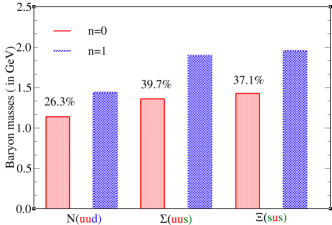
Figure 3: Differences between the ground states and their first radial excitations for light baryons

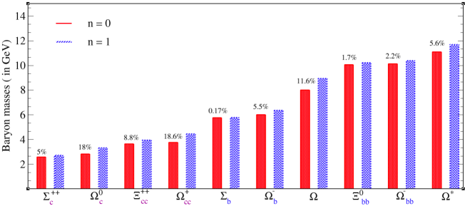
Figure 4: Baryons with spin-$1/2$: Comparison between the masses of the ground states and their first radial excitations. Within each pair of bars, the percentage difference between the masses for states $n=0$ and $n=1$ is indicated.

In Table 3, we display our results for doubly heavy baryons compared with other models, utilizing the QCD sum rules formalism (SM)Shekari Tousi and Azizi (2024), Relativistic quark Model (RQM)Ebert et al. (2002), in a Salpeter model with AdS/QCD inspired potential (SMP) Giannuzzi (2009).

Table 3: The masses of firts radial excitation of the doubly heavy baryons in GeV and comparison of the results with other predictions.

	CI	SM Shekari Tousi and Azizi (2024)	RQM Ebert et al. (2002)	SMP Giannuzzi (2009)
$\Xi_{cc}^{++}({\color[rgb]{1,0,0}u}{\color[rgb]{0.55,0.0,0.55}c}{\color[rgb]{0.55,0.0,0.55}c})$	3.96	4.0	3.91	4.18
$\Omega_{{\color[rgb]{0.55,0.0,0.55}c}{\color[rgb]{0.55,0.0,0.55}c}}^{+}({\color[rgb]{0,0.5,0}s}{\color[rgb]{0.55,0.0,0.55}c}{\color[rgb]{0.55,0.0,0.55}c})$	4.46	4.07	4.08	4.27
$\Xi_{bb}^{0}({\color[rgb]{1,0,0}u}{\color[rgb]{0,0,1}b}{\color[rgb]{0,0,1}b})$	10.24	10.33	10.44	10.75
$\Omega_{bb}^{-}({\color[rgb]{0,0.5,0}s}{\color[rgb]{0,0,1}b}{\color[rgb]{0,0,1}b})$	10.37	10.45	10.61	10.83

Our results for triply heavy baryons with spin-$1/2$ are compared in Table 4 from SM Alomayrah and Barakat (2020), constituent quark model (QM) Yang et al. (2020), the renormalization group procedure for effective particles (EP) Serafin et al. (2018), and RQM Faustov and Galkin (2022); Ebert et al. (2008). Clearly, our results for both states are perfectly consistent with those reported using other models.

Table 4: The masses of first radial excitation of the triply heavy baryons in GeV and comparison of the results with other predictions.

	CI	SM Alomayrah and Barakat (2020)	QM Yang et al. (2020)	EP Serafin et al. (2018)	RQM Faustov and Galkin (2022); Ebert et al. (2008)
$\Omega({\color[rgb]{0.55,0.0,0.55}c}{\color[rgb]{0.55,0.0,0.55}c}{\color[rgb]{0,0,1}b})$	8.94	8.65	8.46	8.6	8.40
$\Omega({\color[rgb]{0.55,0.0,0.55}c}{\color[rgb]{0,0,1}b}{\color[rgb]{0,0,1}b})$	11.71	11.77	11.61	11.59	11.69

The FAs are listed in Table 5, highlighting the dominant diquark in calculating the baryonic mass. At this juncture, we also compare them with the amplitudes obtained for the ground state. From these findings, it becomes apparent that six of the baryons comprised of heavy quarks exhibit altered behavior, wherein the predominant diquark contributing to mass differs between the ground state and the radial excitation. Conversely, only four maintain consistency in behavior.

Table 5: Baryon-$1/2$ FA. Notably, the amplitudes give the dominant diquark in the mass of the baryon. In the last column, we indicate this diquark in each case. The baryons that change their dominant diquark upon transitioning from the ground state to the first radial excitation are $N({\color[rgb]{1,0,0}u}{\color[rgb]{1,0,0}u}{\color[rgb]{0.64,0.0,0.0}d})$, $\Sigma_{{\color[rgb]{0.55,0.0,0.55}c}}^{++}({\color[rgb]{1,0,0}u}{\color[rgb]{1,0,0}u}{\color[rgb]{0.55,0.0,0.55}c})$, $\Xi({\color[rgb]{0,0.5,0}s}{\color[rgb]{1,0,0}u}{\color[rgb]{0,0.5,0}s})$, $\Omega_{{\color[rgb]{0.55,0.0,0.55}c}}^{0}({\color[rgb]{0,0.5,0}s}{\color[rgb]{0,0.5,0}s}{\color[rgb]{0.55,0.0,0.55}c})$, $\Sigma({\color[rgb]{1,0,0}u}{\color[rgb]{1,0,0}u}{\color[rgb]{0,0.5,0}s})$, $\Omega({\color[rgb]{0.55,0.0,0.55}c}{\color[rgb]{0.55,0.0,0.55}c}{\color[rgb]{0,0,1}b})$, $\Xi_{bb}^{0}({\color[rgb]{1,0,0}u}{\color[rgb]{0,0,1}b}{\color[rgb]{0,0,1}b})$, $\Omega_{{\color[rgb]{0,0,1}b}{\color[rgb]{0,0,1}b}}^{-}({\color[rgb]{0,0.5,0}s}{\color[rgb]{0,0,1}b}{\color[rgb]{0,0,1}b})$ and $\Omega({\color[rgb]{0.55,0.0,0.55}c}{\color[rgb]{0,0,1}b}{\color[rgb]{0,0,1}b})$; however, the $\Xi_{cc}^{++}({\color[rgb]{1,0,0}u}{\color[rgb]{0.55,0.0,0.55}c}{\color[rgb]{0.55,0.0,0.55}c})$, $\Omega_{{\color[rgb]{0.55,0.0,0.55}c}{\color[rgb]{0.55,0.0,0.55}c}}^{+}({\color[rgb]{0,0.5,0}s}{\color[rgb]{0.55,0.0,0.55}c}{\color[rgb]{0.55,0.0,0.55}c})$, $\Sigma_{{\color[rgb]{0,0,1}b}^{+}}({\color[rgb]{1,0,0}u}{\color[rgb]{1,0,0}u}{\color[rgb]{0,0,1}b})$ and $\Omega_{{\color[rgb]{0,0,1}b}^{-}}({\color[rgb]{0,0.5,0}s}{\color[rgb]{0,0.5,0}s}{\color[rgb]{0,0,1}b})$ baryons maintain the same behavior as the ground state .

		$s$	$a_{1}^{+}$	$a_{1}^{0}$	$a_{2}^{+}$	$a_{2}^{0}$	dom
$N({\color[rgb]{1,0,0}u}{\color[rgb]{1,0,0}u}{\color[rgb]{0.64,0.0,0.0}d})$	$n=0$	-0.02	0.52	-0.37	-0.63	0.44	$\{{\color[rgb]{1,0,0}u}{\color[rgb]{1,0,0}u}\}{\color[rgb]{0.64,0.0,0.0}d}$
	$n=1$	-0.76	-0.11	0.14	0.50	-0.36	$[{\color[rgb]{1,0,0}u}{\color[rgb]{0.64,0.0,0.0}d}]{\color[rgb]{1,0,0}u}$
$\Sigma({\color[rgb]{1,0,0}u}{\color[rgb]{1,0,0}u}{\color[rgb]{0,0.5,0}s})$	$n=0$	0	-0.04	0.02	0.83	-0.55	$\{{\color[rgb]{1,0,0}u}{\color[rgb]{1,0,0}u}\}{\color[rgb]{0,0.5,0}s}$
	$n=1$	-0.85	-0.20	0.18	0.37	-0.22	$[{\color[rgb]{1,0,0}u}{\color[rgb]{0,0.5,0}s}]{\color[rgb]{1,0,0}u}$
$\Xi({\color[rgb]{0,0.5,0}s}{\color[rgb]{1,0,0}u}{\color[rgb]{0,0.5,0}s})$	$n=0$	0	0.01	-0.99	-0.02	0.06	$\{{\color[rgb]{1,0,0}u}{\color[rgb]{0,0.5,0}s}\}{\color[rgb]{0,0.5,0}s}$
	$n=1$	0.79	0.21	-0.18	-0.47	0.23	$[{\color[rgb]{1,0,0}u}{\color[rgb]{0,0.5,0}s}]{\color[rgb]{0,0.5,0}s}$
$\Sigma_{{\color[rgb]{0.55,0.0,0.55}c}}^{++}({\color[rgb]{1,0,0}u}{\color[rgb]{1,0,0}u}{\color[rgb]{0.55,0.0,0.55}c})$	$n=0$	-0.49	0.26	-0.09	-0.82	0.01	$\{{\color[rgb]{1,0,0}u}{\color[rgb]{1,0,0}u}\}{\color[rgb]{0.55,0.0,0.55}c}$
	$n=1$	0.94	0.27	-0.09	0.12	0.03	$[{\color[rgb]{1,0,0}u}{\color[rgb]{0.55,0.0,0.55}c}]{\color[rgb]{1,0,0}u}$
$\Omega_{{\color[rgb]{0.55,0.0,0.55}c}}^{0}({\color[rgb]{0,0.5,0}s}{\color[rgb]{0,0.5,0}s}{\color[rgb]{0.55,0.0,0.55}c})$	$n=0$	0.57	-0.29	0.10	0.76	-0.02	$\{{\color[rgb]{0,0.5,0}s}{\color[rgb]{0,0.5,0}s}\}{\color[rgb]{0.55,0.0,0.55}c}$
	$n=1$	0.92	0.29	-0.15	0.17	0.07	$[{\color[rgb]{0,0.5,0}s}{\color[rgb]{0.55,0.0,0.55}c}]{\color[rgb]{0,0.5,0}s}$
$\Xi_{cc}^{++}({\color[rgb]{1,0,0}u}{\color[rgb]{0.55,0.0,0.55}c}{\color[rgb]{0.55,0.0,0.55}c})$	$n=0$	-0.88	0.05	-0.36	0.11	0.30	$[{\color[rgb]{1,0,0}u}{\color[rgb]{0.55,0.0,0.55}c}]{\color[rgb]{0.55,0.0,0.55}c}$
	$n=1$	-0.93	-0.04	0.22	0.05	-0.25	$[{\color[rgb]{1,0,0}u}{\color[rgb]{0.55,0.0,0.55}c}]{\color[rgb]{0.55,0.0,0.55}c}$
$\Omega_{{\color[rgb]{0.55,0.0,0.55}c}{\color[rgb]{0.55,0.0,0.55}c}}^{+}({\color[rgb]{0,0.5,0}s}{\color[rgb]{0.55,0.0,0.55}c}{\color[rgb]{0.55,0.0,0.55}c})$	$n=0$	-0.88	0.07	-0.35	0.11	0.30	$[{\color[rgb]{0,0.5,0}s}{\color[rgb]{0.55,0.0,0.55}c}]{\color[rgb]{0.55,0.0,0.55}c}$
	$n=1$	0.90	0.09	-0.31	0.11	0.25	$[{\color[rgb]{0,0.5,0}s}{\color[rgb]{0.55,0.0,0.55}c}]{\color[rgb]{0.55,0.0,0.55}c}$
$\Sigma_{b}^{+}({\color[rgb]{1,0,0}u}{\color[rgb]{1,0,0}u}{\color[rgb]{0,0,1}b})$	$n=0$	0.5	-0.20	0.05	0.83	0.04	$\{{\color[rgb]{1,0,0}u}{\color[rgb]{1,0,0}u}\}{\color[rgb]{0,0,1}b}$
	$n=1$	0.65	0.26	0.01	0.71	-0.02	$\{{\color[rgb]{1,0,0}u}{\color[rgb]{1,0,0}u}\}{\color[rgb]{0,0,1}b}$
$\Omega_{b}^{-}({\color[rgb]{0,0.5,0}s}{\color[rgb]{0,0.5,0}s}{\color[rgb]{0,0,1}b})$	$n=0$	0.12	-0.10	0.04	-0.98	-0.07	$\{{\color[rgb]{0,0.5,0}s}{\color[rgb]{0,0.5,0}s}\}{\color[rgb]{0,0,1}b}$
	$n=1$	0.68	0.22	0.01	0.69	-0.03	$\{{\color[rgb]{0,0.5,0}s}{\color[rgb]{0,0.5,0}s}\}{\color[rgb]{0,0,1}b}$
$\Omega({\color[rgb]{0.55,0.0,0.55}c}{\color[rgb]{0.55,0.0,0.55}c}{\color[rgb]{0,0,1}b})$	$n=0$	-0.82	0.21	-0.008	-0.53	-0.003	$[{\color[rgb]{0.55,0.0,0.55}c}{\color[rgb]{0,0,1}b}]{\color[rgb]{0.55,0.0,0.55}c}$
	$n=1$	0.61	0.38	0.19	0.65	0.08	$\{{\color[rgb]{0.55,0.0,0.55}c}{\color[rgb]{0.55,0.0,0.55}c}\}{\color[rgb]{0,0,1}b}$
$\Xi_{bb}^{0}({\color[rgb]{1,0,0}u}{\color[rgb]{0,0,1}b}{\color[rgb]{0,0,1}b})$	$n=0$	-0.11	0.07	-0.04	0.99	0.06	$\{{\color[rgb]{0,0,1}b}{\color[rgb]{0,0,1}b}\}{\color[rgb]{1,0,0}u}$
	$n=1$	0.98	0.008	-0.12	0.005	0.13	$[{\color[rgb]{1,0,0}u}{\color[rgb]{0,0,1}b}]{\color[rgb]{0,0,1}b}$
$\Omega_{bb}^{-}({\color[rgb]{0,0.5,0}s}{\color[rgb]{0,0,1}b}{\color[rgb]{0,0,1}b})$	$n=0$	0.12	-0.10	0.04	-0.98	-0.07	$\{{\color[rgb]{0,0,1}b}{\color[rgb]{0,0,1}b}\}{\color[rgb]{0,0.5,0}s}$
	$n=1$	-0.96	-0.01	0.16	-0.07	-0.16	$[{\color[rgb]{0,0.5,0}s}{\color[rgb]{0,0,1}b}]{\color[rgb]{0,0,1}b}$
$\Omega({\color[rgb]{0.55,0.0,0.55}c}{\color[rgb]{0,0,1}b}{\color[rgb]{0,0,1}b})$	$n=0$	-0.77	0.05	-0.30	0.49	0.28	$[{\color[rgb]{0.55,0.0,0.55}c}{\color[rgb]{0,0,1}b}]{\color[rgb]{0,0,1}b}$
	$n=1$	0.59	0.07	-0.17	0.72	0.28	$\{{\color[rgb]{0.55,0.0,0.55}c}{\color[rgb]{0,0,1}b}\}{\color[rgb]{0,0,1}b}$

The masses of radial excitations, as well as the masses in the ground state of the baryons, must adhere to the spacing rule. Light baryons satisfy the Gell-Mann–Okubo mass formula Gell-Mann (1962); Okubo (1962):

$$\frac{1}{2}(m_{N({\color[rgb]{1,0,0}u}{\color[rgb]{1,0,0}u}{\color[rgb]{0.64,0.0,0.0}d})}+m_{\Xi({\color[rgb]{0,0.5,0}s}{\color[rgb]{1,0,0}u}{\color[rgb]{0,0.5,0}s})})=\frac{1}{4}(3m_{\Lambda({\color[rgb]{1,0,0}u}{\color[rgb]{0.64,0.0,0.0}d}{\color[rgb]{0,0.5,0}s})}+m_{\Sigma({\color[rgb]{1,0,0}u}{\color[rgb]{1,0,0}u}{\color[rgb]{0,0.5,0}s})})\,.$$ (61)

that predicts a mass of 1.63 GeV for $m_{\Lambda({\color[rgb]{1,0,0}u}{\color[rgb]{0.64,0.0,0.0}d}{\color[rgb]{0,0.5,0}s})}$, which is in remarkably good agreement with the experimental result of 1.60 GeV Nakamura et al. (2010). For baryons with one heavy quark, the spacing rule satisfies Ebert et al. (2005); Gell-Mann (1962); Okubo (1962),

$$m_{\Sigma_{Q}}+m_{\Omega_{Q}}=2m_{\Xi_{Q}}\;,\;\;\;\;\;\;\;\;\;Q={\color[rgb]{0.55,0.0,0.55}c},\;{\color[rgb]{0,0,1}b}\;.$$ (62)

We test this rule for the following baryons :

$$m_{\Sigma_{{\color[rgb]{0.55,0.0,0.55}c}}^{++}({\color[rgb]{1,0,0}u}{\color[rgb]{1,0,0}u}{\color[rgb]{0.55,0.0,0.55}c})}+m_{\Omega_{{\color[rgb]{0.55,0.0,0.55}c}}^{0}({\color[rgb]{0,0.5,0}s}{\color[rgb]{0,0.5,0}s}{\color[rgb]{0.55,0.0,0.55}c})} = 2m_{\Xi_{{\color[rgb]{0.55,0.0,0.55}c}}^{+}{({\color[rgb]{1,0,0}u}{\color[rgb]{0,0.5,0}s}{\color[rgb]{0.55,0.0,0.55}c})}},$$ (63)

$$m_{\Sigma_{{\color[rgb]{0,0,1}b}}^{+}{({\color[rgb]{1,0,0}u}{\color[rgb]{1,0,0}u}{\color[rgb]{0,0,1}b})}}+m_{\Omega_{{\color[rgb]{0,0,1}b}}^{-}{({\color[rgb]{0,0.5,0}s}{\color[rgb]{0,0.5,0}s}{\color[rgb]{0,0,1}b})}} = 2m_{\Xi_{{\color[rgb]{0,0,1}b}}^{0}{({\color[rgb]{1,0,0}u}{\color[rgb]{0,0.5,0}s}{\color[rgb]{0,0,1}b})}}\;.$$ (64)

Using Eqs. (63)-(64) and the results in Table 2, we find $m_{\Xi_{{\color[rgb]{0.55,0.0,0.55}c}}^{+}{({\color[rgb]{1,0,0}u}{\color[rgb]{0,0.5,0}s}{\color[rgb]{0.55,0.0,0.55}c})}}=3.02$ GeV and $m_{\Xi_{{\color[rgb]{0,0,1}b}}^{0}{({\color[rgb]{1,0,0}u}{\color[rgb]{0,0.5,0}s}{\color[rgb]{0,0,1}b})}}=6.125$ GeV. Applying the identical calculation to the predictions derived within the QRS framework yields $m_{\Xi_{{\color[rgb]{0.55,0.0,0.55}c}}^{+}({\color[rgb]{1,0,0}u}{\color[rgb]{0,0.5,0}s}{\color[rgb]{0.55,0.0,0.55}c})}=2.79$ GeV and $m_{\Xi_{{\color[rgb]{0,0,1}b}}^{0}{({\color[rgb]{1,0,0}u}{\color[rgb]{0,0.5,0}s}{\color[rgb]{0,0,1}b})}}=6.055$ GeV. For the proposed state of the first radial excitation of $\Xi_{{\color[rgb]{0,0,1}b}}^{0}({\color[rgb]{1,0,0}u}{\color[rgb]{0,0.5,0}s}{\color[rgb]{0,0,1}b})$, the mass found by LHCb in Refs. Aaij et al. (2018); Aliev et al. (2018) is $6.22$ GeV, remarkably close to the result derived from our model.

IV.2 Fisrt Radial Excitation: Baryons with spin-3/2

Now we focus our attention on the heaviest baryons, which include baryons containing three identical heavy quarks in their configuration.
We show our results for the first radial excitation of these states in Table 6, where, as in the case of spin-1/2 baryons, we have analyzed our results by varying the parameter $g_{B}$. We found that, as in the previous case, the mass increases when $g_{B}$ decreases and decreases when $g_{B}$ increases. We also compared our results with known experimental data Workman and Others (2022), the QRS model Qin et al. (2019), and the ground states calculate by Lattice in Refs. Brown et al. (2014); Mathur et al. (2018) and CI in Refs. Gutiérrez-Guerrero et al. (2019, 2021).

Table 6: Masses of baryons with spin-3/2. Masses from CI in the ground state are taken from Refs. Gutiérrez-Guerrero et al. (2019, 2021). Our results for the first radial excitation with CI are shown in the last column, where we have included the results of varying the parameter $g_{B}\pm 0.5$. Results denoted by QRS have been taken from Ref. Qin et al. (2019), lattice (Lat.) values are taken from Brown et al. (2014); Mathur et al. (2018), and the experimentally results from Ref. Workman and Others (2022).

	$n=0$			$n=1$
Baryon	Lat.	CI	Exp.	Exp.	QRS	CI
$\Delta({\color[rgb]{1,0,0}u}{\color[rgb]{1,0,0}u}{\color[rgb]{1,0,0}u})$	1.23	1.39	1.65	1.60	1.46	$1.67^{-0.07}_{+0.03}$
$\Sigma^{*}({\color[rgb]{1,0,0}u}{\color[rgb]{1,0,0}u}{\color[rgb]{0,0.5,0}s})$	1.39	1.51	1.67	1.73	1.627	$2.01^{-0.02}_{+0.02}$
$\Xi^{*}({\color[rgb]{0,0.5,0}s}{\color[rgb]{1,0,0}u}{\color[rgb]{0,0.5,0}s})$	1.53	1.63	1.82	–	1.793	$2.24^{-0.04}_{+0.05}$
$\Omega({\color[rgb]{0,0.5,0}s}{\color[rgb]{0,0.5,0}s}{\color[rgb]{0,0.5,0}s})$	1.67	1.76	–	–	1.96	$2.25^{-0.04}_{+0.03}$
$\Sigma_{{\color[rgb]{0.55,0.0,0.55}c}}^{++*}{({\color[rgb]{1,0,0}u}{\color[rgb]{1,0,0}u}{\color[rgb]{0.55,0.0,0.55}c})}$	2.52	2.71	–	–	2.80	$2.80^{-0.02}_{+0.04}$
$\Omega_{{\color[rgb]{0.55,0.0,0.55}c}}^{0*}{({\color[rgb]{0,0.5,0}s}{\color[rgb]{0,0.5,0}s}{\color[rgb]{0.55,0.0,0.55}c})}$	2.76	2.90	–	–	3.02	$3.26^{-0.02}_{+0.05}$
$\Xi_{{\color[rgb]{0.55,0.0,0.55}c}{\color[rgb]{0.55,0.0,0.55}c}}^{++*}{({\color[rgb]{1,0,0}u}{\color[rgb]{0.55,0.0,0.55}c}{\color[rgb]{0.55,0.0,0.55}c})}$	3.57	3.76	–	–	3.97	$4.30^{-0.02}_{+0.03}$
$\Omega_{{\color[rgb]{0.55,0.0,0.55}c}{\color[rgb]{0.55,0.0,0.55}c}}^{+*}{({\color[rgb]{0,0.5,0}s}{\color[rgb]{0.55,0.0,0.55}c}{\color[rgb]{0.55,0.0,0.55}c})}$	3.71	3.90	–	–	4.08	$4.54^{-0.01}_{+0.04}$
$\Sigma_{{\color[rgb]{0,0,1}b}}^{+*}{({\color[rgb]{1,0,0}u}{\color[rgb]{1,0,0}u}{\color[rgb]{0,0,1}b})}$	5.75	5.85	–	–	6.07	$5.89$${}^{-0.04}_{+0.03}$
$\Omega_{{\color[rgb]{0,0,1}b}}^{-*}{({\color[rgb]{0,0.5,0}s}{\color[rgb]{0,0.5,0}s}{\color[rgb]{0,0,1}b})}$	5.99	6.09	–	–	6.30	$6.41$${}^{-0.03}_{+0.01}$
$\Xi_{bb}^{0*}{({\color[rgb]{1,0,0}u}{\color[rgb]{0,0,1}b}{\color[rgb]{0,0,1}b})}$	10.04	10.09	–	–	10.52	$10.42^{-0.01}_{+0.04}$
$\Omega_{{\color[rgb]{0,0,1}b}{\color[rgb]{0,0,1}b}}^{-*}{({\color[rgb]{0,0.5,0}s}{\color[rgb]{0,0,1}b}{\color[rgb]{0,0,1}b})}$	10.18	10.20	–	–	10.64	$10.67^{-0.02}_{+0.01}$
$\Omega_{{\color[rgb]{0.55,0.0,0.55}c}{\color[rgb]{0.55,0.0,0.55}c}{\color[rgb]{0.55,0.0,0.55}c}}^{++*}$	4.80	4.93	–	–	5.15	$5.59^{-0.03}_{+0.01}$
$\Omega_{{\color[rgb]{0.55,0.0,0.55}c}{\color[rgb]{0.55,0.0,0.55}c}{\color[rgb]{0,0,1}b}}^{+*}$	8.01	8.03	–	–	8.42	$8.64^{-0.02}_{+0.01}$
$\Omega_{{\color[rgb]{0.55,0.0,0.55}c}{\color[rgb]{0,0,1}b}{\color[rgb]{0,0,1}b}}^{0*}$	11.20	11.12	–	–	11.70	$11.66^{-0.01}_{+0.02}$
$\Omega_{{\color[rgb]{0,0,1}b}{\color[rgb]{0,0,1}b}{\color[rgb]{0,0,1}b}}^{-*}$	14.37	14.23	–	–	14.98	$14.66^{-0.01}_{+0.01}$

In Figs. 5 and 6, we have plotted the masses reported in Table 6 to represent these values visually, similar to the case of baryons with spin-$1/2$, along with their percentage differences. It is readily apparent that all radial excitations surpass their ground states. Furthermore, in the heavy sector the largest discrepancy is observed for $\Omega_{{\color[rgb]{0.55,0.0,0.55}c}{\color[rgb]{0.55,0.0,0.55}c}}^{+*}{({\color[rgb]{0,0.5,0}s}{\color[rgb]{0.55,0.0,0.55}c}{\color[rgb]{0.55,0.0,0.55}c})}$ at 16.4%, while the smallest is seen for $\Sigma_{{\color[rgb]{0,0,1}b}}^{+*}{({\color[rgb]{1,0,0}u}{\color[rgb]{1,0,0}u}{\color[rgb]{0,0,1}b})}$ at 0.67%. Of particular significance is the outcome for $\Omega_{{\color[rgb]{0.55,0.0,0.55}c}}^{0*}$, LHCb proposes a mass of 3.3 GeV for this state in Refs. Karliner and Rosner (2023); Aaij et al. (2023); Pan and Pan (2024), while our CI model yields 3.26 GeV presenting a small difference of approximately 1.21%.

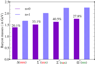
Figure 5: Comparison between the masses of the ground states and their first radial excitations for light baryons.

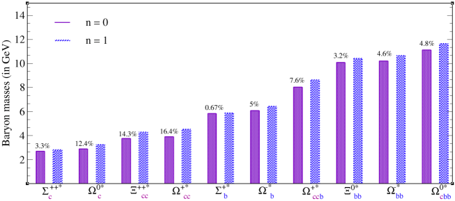
Figure 6: Baryons with spin-3/2: Comparison between the masses of their ground states and their first radial excitations. Within each pair of bars, the percentage difference between the masses for states $n=0$ and $n=1$ is indicated.

In Table 7, we present the heaviest baryons with spin-3/2, comprised of two and three ${\color[rgb]{0,0,1}b}$ and ${\color[rgb]{0.55,0.0,0.55}c}$ quarks. Additionally, we also display results for these baryons obtained using alternative models, QRS Qin et al. (2019), RQM Faustov and Galkin (2022); Ebert et al. (2008) and Regge phenomenology (RF) Oudichhya et al. (2023); Shah and Rai (2017b).

Table 7: Masses of triple heavy baryons with spin-$3/2$, compared to the masses predicted by other models.

Baryon	CI	QRS Qin et al. (2019)	RQM Faustov and Galkin (2022); Ebert et al. (2008)	RF Oudichhya et al. (2023); Shah and Rai (2017b)
$\Omega_{{\color[rgb]{0.55,0.0,0.55}c}{\color[rgb]{0.55,0.0,0.55}c}{\color[rgb]{0,0,1}b}}^{+*}$	8.64	8.42	8.41	8.63
$\Omega_{{\color[rgb]{0.55,0.0,0.55}c}{\color[rgb]{0,0,1}b}{\color[rgb]{0,0,1}b}}^{0*}$	11.66	11.70	11.70	11.79
$\Omega_{{\color[rgb]{0.55,0.0,0.55}c}{\color[rgb]{0.55,0.0,0.55}c}{\color[rgb]{0.55,0.0,0.55}c}}^{++*}$	5.59	5.15	5.54	5.3
$\Omega_{{\color[rgb]{0,0,1}b}{\color[rgb]{0,0,1}b}{\color[rgb]{0,0,1}b}}^{-*}$	14.66	14.98	15.12	15.16

To conduct a visual analysis of these baryons within Figs. 7 and 8, we delineate the triple baryons composed of ${\color[rgb]{0.55,0.0,0.55}c}{\color[rgb]{0.55,0.0,0.55}c}{\color[rgb]{0.55,0.0,0.55}c}$ and ${\color[rgb]{0,0,1}b}{\color[rgb]{0,0,1}b}{\color[rgb]{0,0,1}b}$. The left panel illustrates the baryon ground states, while the right panel depicts their first radial excitation. This graphical representation facilitates a direct comparison with alternative approaches.
In Tables 6 and 7, we emphasize that the results obtained with CI in the ground state and the first excited state are consistent with other models, such as lattice and QRS.
We define a constituent-quark passive-mass in analogy with the ground state of baryons Qin et al. (2018); Gutiérrez-Guerrero et al. (2019), via

$$M_{f}^{P} = \frac{1}{3}m_{\Omega_{fff}}\,.$$ (65)

In Table 8, we compare the computed values (in GeV) from this relation with the input parameters we used for CI in the ground and first radial excitation. This mass increases when we transition from $n=0$ to $n=1$, just as expected.

Table 8: Constituent-quark passive-mass derived from CI, Lattice, and the QRS model, corresponding to states $n=0$ and $n=1$.

			${\color[rgb]{0.55,0.0,0.55}c}$	${\color[rgb]{0,0,1}b}$
		$M_{f}$	$1.53$	$4.68$
$n=0$	CI	$M_{f}^{P}$	1.64	4.74
	Lat.	$M_{f}^{P}$	1.6	4.79
$n=1$	CI	$M_{f}^{P}$	1.86	4.88
	QRS	$M_{f}^{P}$	1.71	4.99

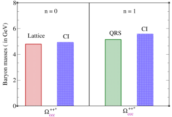
Figure 7: Comparison between the masses of the ground states and their first radial excitations for $\Omega^{++*}_{{\color[rgb]{0.55,0.0,0.55}c}{\color[rgb]{0.55,0.0,0.55}c}{\color[rgb]{0.55,0.0,0.55}c}}$.

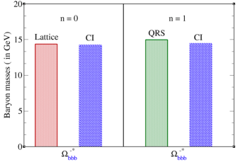
Figure 8: Comparison between the masses of the ground states and their first radial excitations for $\Omega^{-*}_{{\color[rgb]{0,0,1}b}{\color[rgb]{0,0,1}b}{\color[rgb]{0,0,1}b}}$.

The masses of baryons with spin-$3/2$ with a single heavy quark obey an equal-spacing rule Ebert et al. (2005); Gell-Mann (1962); Okubo (1962)

$$m_{\Sigma_{Q}}+m_{\Omega_{Q}}=2m_{\Xi_{Q}}\,.\;\;\;\;\;\;\;\;\;Q={\color[rgb]{0.55,0.0,0.55}c},\;{\color[rgb]{0,0,1}b}$$ (66)

This relation yields a mass of $m_{\Xi_{{\color[rgb]{1,0,0}u}{\color[rgb]{0,0.5,0}s}{\color[rgb]{0.55,0.0,0.55}c}}}=3.03$ GeV. For the corresponding baryon containing a bottom quark, we obtain $m_{\Xi_{{\color[rgb]{1,0,0}u}{\color[rgb]{0,0.5,0}s}{\color[rgb]{0,0,1}b}}}=6.19$ GeV.
We now turn our attention to the spacing rules which combine baryons with different spins Yu and Guo (2018) :

$$m_{\Xi_{{\color[rgb]{0.55,0.0,0.55}c}{\color[rgb]{0.55,0.0,0.55}c}}^{++*}{({\color[rgb]{1,0,0}u}{\color[rgb]{0.55,0.0,0.55}c}{\color[rgb]{0.55,0.0,0.55}c})}}-m_{\Xi_{{\color[rgb]{0.55,0.0,0.55}c}{\color[rgb]{0.55,0.0,0.55}c}}^{++}({\color[rgb]{1,0,0}u}{\color[rgb]{0.55,0.0,0.55}c}{\color[rgb]{0.55,0.0,0.55}c})}-m_{\Sigma_{{\color[rgb]{0.55,0.0,0.55}c}}^{++*}{({\color[rgb]{1,0,0}u}{\color[rgb]{1,0,0}u}{\color[rgb]{0.55,0.0,0.55}c})}}+m_{\Sigma_{{\color[rgb]{0.55,0.0,0.55}c}}^{++}({\color[rgb]{1,0,0}u}{\color[rgb]{1,0,0}u}{\color[rgb]{0.55,0.0,0.55}c})}=0\,,$$ (67)

$$m_{\Omega_{cc}^{+*}{({\color[rgb]{0,0.5,0}s}{\color[rgb]{0.55,0.0,0.55}c}{\color[rgb]{0.55,0.0,0.55}c})}}-m_{\Omega_{{\color[rgb]{0.55,0.0,0.55}c}{\color[rgb]{0.55,0.0,0.55}c}}^{+}({\color[rgb]{0,0.5,0}s}{\color[rgb]{0.55,0.0,0.55}c}{\color[rgb]{0.55,0.0,0.55}c})}-m_{\Omega_{{\color[rgb]{0.55,0.0,0.55}c}}^{0*}{({\color[rgb]{0,0.5,0}s}{\color[rgb]{0,0.5,0}s}{\color[rgb]{0.55,0.0,0.55}c})}}+m_{\Omega_{{\color[rgb]{0.55,0.0,0.55}c}}^{0}({\color[rgb]{0,0.5,0}s}{\color[rgb]{0,0.5,0}s}{\color[rgb]{0.55,0.0,0.55}c})}=0\,,$$ (68)

$$m_{\Xi_{{\color[rgb]{0,0,1}b}{\color[rgb]{0,0,1}b}}^{0*}{({\color[rgb]{1,0,0}u}{\color[rgb]{0,0,1}b}{\color[rgb]{0,0,1}b})}}-m_{\Xi_{{\color[rgb]{0,0,1}b}{\color[rgb]{0,0,1}b}}^{0}({\color[rgb]{1,0,0}u}{\color[rgb]{0,0,1}b}{\color[rgb]{0,0,1}b})}-m_{\Sigma_{{\color[rgb]{0,0,1}b}}^{+*}{({\color[rgb]{1,0,0}u}{\color[rgb]{1,0,0}u}{\color[rgb]{0,0,1}b})}}+m_{\Sigma_{{\color[rgb]{0,0,1}b}}^{+}({\color[rgb]{1,0,0}u}{\color[rgb]{1,0,0}u}{\color[rgb]{0,0,1}b})}=0\,.$$ (69)

Using the results for the masses from Tables 2 and 6 for CI, we obtain, 0.25 GeV, 0.15 GeV and 0.08 GeV for Eqs. (67)-(69) respectively. For completeness and enhanced analysis of the first radial excitations of baryons composed of heavy quarks, we enumerate the FAs in Table 9 while also highlighting the dominant diquark in each baryon.

Table 9: FAs for spin-$3/2$ baryons. According to our analysis, the dominant diquarks are listed in the last column. The baryons that change their dominant diquark upon transitioning from the ground state to the first radial excitation are $\Omega_{{\color[rgb]{0.55,0.0,0.55}c}{\color[rgb]{0.55,0.0,0.55}c}}^{+*}{({\color[rgb]{0,0.5,0}s}{\color[rgb]{0.55,0.0,0.55}c}{\color[rgb]{0.55,0.0,0.55}c})}$, $\Sigma_{{\color[rgb]{0,0,1}b}}^{+*}{({\color[rgb]{1,0,0}u}{\color[rgb]{1,0,0}u}{\color[rgb]{0,0,1}b})}$, $\Omega_{{\color[rgb]{0,0,1}b}}^{-*}{({\color[rgb]{0,0.5,0}s}{\color[rgb]{0,0.5,0}s}{\color[rgb]{0,0,1}b})}$ $\Omega_{{\color[rgb]{0.55,0.0,0.55}c}{\color[rgb]{0.55,0.0,0.55}c}{\color[rgb]{0,0,1}b}}^{+*}$, ; however, the $\Sigma^{*}({\color[rgb]{1,0,0}u}{\color[rgb]{1,0,0}u}{\color[rgb]{0,0.5,0}s})$, $\Sigma^{*}({\color[rgb]{1,0,0}u}{\color[rgb]{1,0,0}u}{\color[rgb]{0,0.5,0}s})$, $\Omega_{{\color[rgb]{0.55,0.0,0.55}c}}^{0*}{({\color[rgb]{0,0.5,0}s}{\color[rgb]{0,0.5,0}s}{\color[rgb]{0.55,0.0,0.55}c})}$, $\Xi_{{\color[rgb]{0.55,0.0,0.55}c}{\color[rgb]{0.55,0.0,0.55}c}}^{++*}{({\color[rgb]{1,0,0}u}{\color[rgb]{0.55,0.0,0.55}c}{\color[rgb]{0.55,0.0,0.55}c})}$, $\Sigma_{{\color[rgb]{0.55,0.0,0.55}c}}^{++*}{({\color[rgb]{1,0,0}u}{\color[rgb]{1,0,0}u}{\color[rgb]{0.55,0.0,0.55}c})}$, $\Xi_{{\color[rgb]{0,0,1}b}{\color[rgb]{0,0,1}b}}^{0*}{({\color[rgb]{1,0,0}u}{\color[rgb]{0,0,1}b}{\color[rgb]{0,0,1}b})}$, $\Omega_{{\color[rgb]{0,0,1}b}{\color[rgb]{0,0,1}b}}^{-*}{({\color[rgb]{0,0.5,0}s}{\color[rgb]{0,0,1}b}{\color[rgb]{0,0,1}b})}$, and $\Omega_{{\color[rgb]{0.55,0.0,0.55}c}{\color[rgb]{0,0,1}b}{\color[rgb]{0,0,1}b}}^{0*}$ baryons maintain the same behavior as the ground state.

		$d^{\{qq_{1}\}}$	$d^{\{qq\}}$	dom.
$\Sigma^{*}({\color[rgb]{1,0,0}u}{\color[rgb]{1,0,0}u}{\color[rgb]{0,0.5,0}s})$	$n=0$	0.25	0.96	$\{{\color[rgb]{1,0,0}u}{\color[rgb]{1,0,0}u}\}{\color[rgb]{0,0.5,0}s}$
	$n=1$	-0.67	-0.73	$\{{\color[rgb]{1,0,0}u}{\color[rgb]{1,0,0}u}\}{\color[rgb]{0,0.5,0}s}$
$\Xi^{*}({\color[rgb]{0,0.5,0}s}{\color[rgb]{1,0,0}u}{\color[rgb]{0,0.5,0}s})$	$n=0$	0.42	0.90	$\{{\color[rgb]{0,0.5,0}s}{\color[rgb]{0,0.5,0}s}\}{\color[rgb]{1,0,0}u}$
	$n=1$	-0.68	-0.72	$\{{\color[rgb]{0,0.5,0}s}{\color[rgb]{0,0.5,0}s}\}{\color[rgb]{1,0,0}u}$
$\Sigma_{{\color[rgb]{0.55,0.0,0.55}c}}^{++*}{({\color[rgb]{1,0,0}u}{\color[rgb]{1,0,0}u}{\color[rgb]{0.55,0.0,0.55}c})}$	$n=0$	-0.67	-0.74	$\{{\color[rgb]{1,0,0}u}{\color[rgb]{1,0,0}u}\}{\color[rgb]{0.55,0.0,0.55}c}$
	$n=1$	-0.68	-0.72	$\{{\color[rgb]{1,0,0}u}{\color[rgb]{1,0,0}u}\}{\color[rgb]{0.55,0.0,0.55}c}$
$\Omega_{{\color[rgb]{0.55,0.0,0.55}c}}^{0*}{({\color[rgb]{0,0.5,0}s}{\color[rgb]{0,0.5,0}s}{\color[rgb]{0.55,0.0,0.55}c})}$	$n=0$	-0.60	-0.80	$\{{\color[rgb]{0,0.5,0}s}{\color[rgb]{0,0.5,0}s}\}{\color[rgb]{0.55,0.0,0.55}c}$
	$n=1$	-0.67	-0.73	$\{{\color[rgb]{0,0.5,0}s}{\color[rgb]{0,0.5,0}s}\}{\color[rgb]{0.55,0.0,0.55}c}$
$\Xi_{{\color[rgb]{0.55,0.0,0.55}c}{\color[rgb]{0.55,0.0,0.55}c}}^{++*}{({\color[rgb]{1,0,0}u}{\color[rgb]{0.55,0.0,0.55}c}{\color[rgb]{0.55,0.0,0.55}c})}$	$n=0$	-0.12	-0.99	$\{{\color[rgb]{0.55,0.0,0.55}c}{\color[rgb]{0.55,0.0,0.55}c}\}{\color[rgb]{1,0,0}u}$
	$n=1$	-0.68	-0.73	$\{{\color[rgb]{0.55,0.0,0.55}c}{\color[rgb]{0.55,0.0,0.55}c}\}{\color[rgb]{1,0,0}u}$
$\Omega_{{\color[rgb]{0.55,0.0,0.55}c}{\color[rgb]{0.55,0.0,0.55}c}}^{+*}{({\color[rgb]{0,0.5,0}s}{\color[rgb]{0.55,0.0,0.55}c}{\color[rgb]{0.55,0.0,0.55}c})}$	$n=0$	-0.17	-0.99	$\{{\color[rgb]{0.55,0.0,0.55}c}{\color[rgb]{0.55,0.0,0.55}c}\}{\color[rgb]{0,0.5,0}s}$
	$n=1$	-0.73	-0.67	$\{{\color[rgb]{0.55,0.0,0.55}c}{\color[rgb]{0,0.5,0}s}\}{\color[rgb]{0.55,0.0,0.55}c}$
$\Sigma_{{\color[rgb]{0,0,1}b}}^{+*}{({\color[rgb]{1,0,0}u}{\color[rgb]{1,0,0}u}{\color[rgb]{0,0,1}b})}$	$n=0$	-0.56	-0.83	$\{{\color[rgb]{1,0,0}u}{\color[rgb]{1,0,0}u}\}{\color[rgb]{0,0,1}b}$
	$n=1$	-0.79	-0.60	$\{{\color[rgb]{1,0,0}u}{\color[rgb]{0,0,1}b}\}{\color[rgb]{1,0,0}u}$
$\Omega_{{\color[rgb]{0,0,1}b}}^{-*}{({\color[rgb]{0,0.5,0}s}{\color[rgb]{0,0.5,0}s}{\color[rgb]{0,0,1}b})}$	$n=0$	-0.42	-0.90	$\{{\color[rgb]{0,0.5,0}s}{\color[rgb]{0,0.5,0}s}\}{\color[rgb]{0,0,1}b}$
	$n=1$	-0.73	-0.67	$\{{\color[rgb]{0,0.5,0}s}{\color[rgb]{0,0,1}b}\}{\color[rgb]{0,0.5,0}s}$
$\Xi_{{\color[rgb]{0,0,1}b}{\color[rgb]{0,0,1}b}}^{0*}{({\color[rgb]{1,0,0}u}{\color[rgb]{0,0,1}b}{\color[rgb]{0,0,1}b})}$	$n=0$	0.03	0.99	$\{{\color[rgb]{0,0,1}b}{\color[rgb]{0,0,1}b}\}{\color[rgb]{1,0,0}u}$
	$n=1$	-0.34	-0.9	$\{{\color[rgb]{0,0,1}b}{\color[rgb]{0,0,1}b}\}{\color[rgb]{1,0,0}u}$
$\Omega_{{\color[rgb]{0,0,1}b}{\color[rgb]{0,0,1}b}}^{-*}{({\color[rgb]{0,0.5,0}s}{\color[rgb]{0,0,1}b}{\color[rgb]{0,0,1}b})}$	$n=0$	-0.02	-0.99	$\{{\color[rgb]{0,0,1}b}{\color[rgb]{0,0,1}b}\}{\color[rgb]{0,0.5,0}s}$
	$n=1$	-0.40	-0.91	$\{{\color[rgb]{0,0,1}b}{\color[rgb]{0,0,1}b}\}{\color[rgb]{0,0.5,0}s}$
$\Omega_{{\color[rgb]{0.55,0.0,0.55}c}{\color[rgb]{0.55,0.0,0.55}c}{\color[rgb]{0,0,1}b}}^{+*}$	$n=0$	-0.35	-0.93	$\{{\color[rgb]{0.55,0.0,0.55}c}{\color[rgb]{0.55,0.0,0.55}c}\}{\color[rgb]{0,0,1}b}$
	$n=1$	-0.92	-0.38	$\{{\color[rgb]{0.55,0.0,0.55}c}{\color[rgb]{0,0,1}b}\}{\color[rgb]{0.55,0.0,0.55}c}$
$\Omega_{{\color[rgb]{0.55,0.0,0.55}c}{\color[rgb]{0,0,1}b}{\color[rgb]{0,0,1}b}}^{0*}$	$n=0$	-0.16	-0.99	$\{{\color[rgb]{0,0,1}b}{\color[rgb]{0,0,1}b}\}{\color[rgb]{0.55,0.0,0.55}c}$
	$n=1$	-0.22	-0.97	$\{{\color[rgb]{0,0,1}b}{\color[rgb]{0,0,1}b}\}{\color[rgb]{0.55,0.0,0.55}c}$

Analogously to the case of baryons with spin-1/2, baryons with spin-3/2 change the dominant diquark in four cases when transitioning from the ground state to the excited state.

V Conclusions

In this paper, we utilize the CI model to compute the mass spectra of singly, doubly, and triply heavy baryons. The approach includes a quark-diquark approximation to simplify the complex three-body problem into two simpler two-body problems. In this respect, we employed the excited diquarks previously obtained with CI in Ref. Paredes-Torres et al. (2024) and integrated them into the Faddeev equation described in Section II, Fig. 1. In Tables 2 and 6, we present the masses predicted by our model using the parameters described throughout our article and in the appendices. These predictions are compared in Figs. 4 and 6 with the masses in the ground estate. Additionally, in Tables 5 and 9, we have included the FAs for all the baryons studied here.
The predictions obtained in this work with CI for light baryons with spin $1/2$ satisfy the well-known Gell-Mann–Okubo mass formula Gell-Mann (1962); Okubo (1962) in Eq. (61). In the case of baryons with a singly heavy quark ($\Sigma_{{\color[rgb]{0.55,0.0,0.55}c}}^{++},\Omega_{{\color[rgb]{0.55,0.0,0.55}c}}^{0},\Sigma_{{\color[rgb]{0,0,1}b}}^{+},\Omega_{{\color[rgb]{0,0,1}b}}^{-},\Sigma_{{\color[rgb]{0.55,0.0,0.55}c}}^{++*},\Omega_{{\color[rgb]{0.55,0.0,0.55}c}}^{0*},\Sigma_{{\color[rgb]{0,0,1}b}}^{+*},\Omega_{{\color[rgb]{0,0,1}b}}^{-*}$) our results are consistent with those detected by LHCb Aaij et al. (2018, 2020, 2023) and satisfy the mass spacing rule Ebert et al. (2005); Gell-Mann (1962); Okubo (1962) in Eqs. (63), (64) and (66). For baryons with spin-$1/2$ and double heavy quarks, we compare results obtained using other models in Table 3. Results are very close and consistent with existing theoretical predictions. Our results for baryons with two heavy quarks with different spins also satisfy the relations in the Eqs. (67)-(69). Tables 4 and 7 compare the results obtained here for triply heavy baryons with those obtained using other approaches. Furthermore, in Figs. 7 and 8, we plot the masses of baryons composed of three quarks ${\color[rgb]{0,0,1}b}$ and ${\color[rgb]{0.55,0.0,0.55}c}$, comparing them with other models and their ground states. In conclusion, we computed the masses of radial excitations for twenty states composed of heavy quarks and provided the corresponding FAs for each state. This lays the groundwork for subsequent calculations of form factors, charge radii, decay constants, and other observables for baryons. Also, this study will undoubtedly assist future experimental investigations in identifying baryonic states through resonances.

Appendix A Euclidean Conventions

In our Euclidean formulation:

$$p\cdot q=\sum_{i=1}^{4}p_{i}q_{i}\,;$$ (A.1)

where

$$\{\gamma_{\mu},\gamma_{\nu}\}=2\,\delta_{\mu\nu}\,;\;\gamma_{\mu}^{\dagger}=\gamma_{\mu}\,;\;\sigma_{\mu\nu}=\frac{i}{2}[\gamma_{\mu},\gamma_{\nu}]\,;\;$$

$${\rm tr}\,[\gamma_{5}\gamma_{\mu}\gamma_{\nu}\gamma_{\rho}\gamma_{\sigma}]=-4\,\epsilon_{\mu\nu\rho\sigma}\,,\epsilon_{1234}=1\,.$$ (A.2)

A positive energy spinor satisfies

$$\bar{u}(P,s)\,(i\gamma\cdot P+M)=0=(i\gamma\cdot P+M)\,u(P,s)\,,$$ (A.3)

where $s=\pm$ is the spin label. It is normalised as :

$$\bar{u}(P,s)\,u(P,s)=2M\,,$$ (A.4)

and may be expressed explicitly as :

$$u(P,s)=\sqrt{M-i{\cal E}}\left(\begin{array}[]{c}\chi_{s}\\ \displaystyle\frac{\vec{\sigma}\cdot\vec{P}}{M-i{\cal E}}\chi_{s}\end{array}\right)\,,$$ (A.5)

with ${\cal E}=i\sqrt{\vec{P}^{2}+M^{2}}$,

$$\chi_{+}=\left(\begin{array}[]{c}1\\ 0\end{array}\right)\,,\;\chi_{-}=\left(\begin{array}[]{c}0\\ 1\end{array}\right)\,.$$ (A.6)

For the free-particle spinor, $\bar{u}(P,s)=u(P,s)^{\dagger}\gamma_{4}$. It can be used to construct a positive energy projection operator:

$$\Lambda_{+}(P):=\frac{1}{2M}\,\sum_{s=\pm}\,u(P,s)\,\bar{u}(P,s)=\frac{1}{2M}\left(-i\gamma\cdot P+M\right).$$ (A.7)

A negative energy spinor satisfies

$$\bar{v}(P,s)\,(i\gamma\cdot P-M)=0=(i\gamma\cdot P-M)\,v(P,s)\,,$$ (A.8)

and possesses properties and satisfies constraints obtained through obvious analogy with $u(P,s)$. A charge-conjugated BSA is obtained via

$$\bar{\Gamma}(k;P)=C^{\dagger}\,\Gamma(-k;P)^{\rm T}\,C\,,$$ (A.9)

where “T” denotes transposing all matrix indices and $C=\gamma_{2}\gamma_{4}$ is the charge conjugation matrix, $C^{\dagger}=-C$. Moreover, we note that

$$C^{\dagger}\gamma_{\mu}^{\rm T}\,C=-\gamma_{\mu}\,,\;[C,\gamma_{5}]=0\,.$$ (A.10)

We employ a Rarita-Schwinger spinor to represent a covariant spin-$3/2$ field. The positive energy spinor is defined by the following equations:

$$(i\gamma\cdot P+M)\,u_{\mu}(P;r)=0\,,\gamma_{\mu}u_{\mu}(P;r)=0\,,P_{\mu}u_{\mu}(P;r)=0,$$ (A.11)

where $r=-3/2,-1/2,1/2,3/2$. It is normalised as:

$$\bar{u}_{\mu}(P;r^{\prime})\,u_{\mu}(P;r)=2M\,,$$ (A.12)

and satisfies a completeness relation

$$\frac{1}{2M}\sum_{r=-3/2}^{3/2}u_{\mu}(P;r)\,\bar{u}_{\nu}(P;r)=\Lambda_{+}(P)\,R_{\mu\nu}\,,$$ (A.13)

where

$$R_{\mu\nu}=\delta_{\mu\nu}\mbox{\boldmath$I$}_{\rm D}-\frac{1}{3}\gamma_{\mu}\gamma_{\nu}+\frac{2}{3}\hat{P}_{\mu}\hat{P}_{\nu}\mbox{\boldmath$I$}_{\rm D}-i\frac{1}{3}[\hat{P}_{\mu}\gamma_{\nu}-\hat{P}_{\nu}\gamma_{\mu}]\,,$$ (A.14)

with $\hat{P}^{2}=-1$. It is very useful in simplifying the FE for a positive energy decouplet state.

Appendix B Contact interaction: features

The gap equation for fermions requires modelling the gluon propagator and the quark-gluon vertex. Here we shall recall and list these key characteristics of the CI Gutierrez-Guerrero et al. (2010); Roberts et al. (2010); Roberts et al. (2011b, a) :

• The gluon propagator is defined to be independent of any varying momentum scale:

  $$g^{2}D_{\mu\nu}(k) = \frac{4\pi\alpha_{\mathrm{IR}}}{m_{g}^{2}}\delta_{\mu\nu}\equiv\frac{1}{m_{G}^{2}}\delta_{\mu\nu},$$ (B.15)

  where $m_{g}=500\,\text{MeV}$ is a gluon mass scale generated dynamically in QCD Boucaud et al. (2012); Aguilar et al. (2018); Binosi and Papavassiliou (2018); Gao et al. (2018), and $\alpha_{\mathrm{IR}}$ can be interpreted as the interaction strength in the infrared Binosi et al. (2017); Deur et al. (2016); Rodríguez-Quintero et al. (2018).

• At leading-order, the quark-gluon vertex is

  $$\Gamma_{\nu}(p,q)=\gamma_{\nu}$$ (B.16)

• With this kernel the dressed-quark propagator for a quark of flavor $f$ becomes

  $$S_{f}^{-1}(p)=$$

  $$i\gamma\cdot p+m_{f}+\frac{16\pi}{3}\frac{\alpha_{\rm IR}}{m_{G}^{2}}\int\!\frac{d^{4}q}{(2\pi)^{4}}\,\gamma_{\mu}\,S_{f}(q)\,\gamma_{\mu}\,,$$ (B.17)

  where $m_{f}$ is the current-quark mass. The integral possesses quadratic and logarithmic divergences and we regularize them in a Poincaré covariant manner. The solution of this equation is :

  $$S_{f}^{-1}(p)=i\gamma\cdot p+M_{f}\,,$$ (B.18)

  where $M_{f}$ is, in general a mass function running with a momentum scale, but within the CI it is a constant dressed mass.

• $M_{f}$ is determined by

  $$M_{f}=m_{f}+M_{f}\frac{4\alpha_{\rm IR}}{3\pi m_{G}^{2}}\,\,{\cal C}^{\rm iu}(M_{f}^{2})\,,$$ (B.19)

  where

  $$\hskip 21.33955pt{\cal C}^{\rm iu}(\sigma)/\sigma=\overline{\cal C}^{\rm iu}(\sigma)=\Gamma(-1,\sigma\tau_{\rm UV}^{2})-\Gamma(-1,\sigma\tau_{\rm IR}^{2}),$$

  (B.20)

  with $\Gamma(\alpha,y)$ being the incomplete gamma-function and $\tau_{\rm IR,UV}$ are respectively, infrared and ultraviolet regulators. A nonzero value for $\tau_{\mathrm{IR}}\equiv 1/\Lambda_{\mathrm{IR}}$ implements confinement Roberts (2008). Since the CI is a nonrenormalizable theory, $\tau_{\mathrm{UV}}\equiv 1/\Lambda_{\mathrm{UV}}$ becomes part of the model and therefore sets the scale for all dimensional quantities.

In this work we report results using the parameter set in Table 10.

Table 10: Dimensionless coupling constant $\hat{\alpha}=\hat{\alpha}_{\mathrm{I}R}\Lambda_{\mathrm{U}V}^{2}$, where $\hat{\alpha}_{\mathrm{IR}}=\alpha_{\mathrm{IR}}/m_{g}^{2}$, for the CI, extracted from a best-fit to data, as explained in Ref. Raya et al. (2017). Fixed parameters are $m_{g}~{}=~{}0.50~{}\text{GeV}$ and $\Lambda_{\mathrm{IR}}=0.24\,\text{GeV}$.

quarks	$\hat{\alpha}_{\mathrm{IR}}\;[\text{GeV}^{-2}]$	$\Lambda_{\mathrm{UV}}\;[\text{GeV}]$
${\color[rgb]{1,0,0}u}$, ${\color[rgb]{0.64,0.0,0.0}d}$, ${\color[rgb]{0,0.5,0}s}$	1.14	0.91
${\color[rgb]{0.55,0.0,0.55}c},{\color[rgb]{0.64,0.0,0.0}d},{\color[rgb]{0,0.5,0}s}$	0.38	1.32
${\color[rgb]{0.55,0.0,0.55}c}$	0.09	2.31
${\color[rgb]{0,0,1}b},{\color[rgb]{1,0,0}u},{\color[rgb]{0,0.5,0}s}$	0.07	2.52
${\color[rgb]{0,0,1}b},{\color[rgb]{0.55,0.0,0.55}c}$	0.02	4.13
${\color[rgb]{0,0,1}b}$	0.007	6.56

Table 11 presents the values of ${\color[rgb]{1,0,0}u}$, ${\color[rgb]{0,0.5,0}s}$, ${\color[rgb]{0.55,0.0,0.55}c}$ and ${\color[rgb]{0,0,1}b}$ dressed quark masses computed from Eq. (B.19).

Table 11: Computed dressed-quark masses (in GeV), required as input for the BS equation and FE.

$m_{{\color[rgb]{1,0,0}u}}=0.007$	$m_{{\color[rgb]{0,0.5,0}s}}=0.17$	$m_{{\color[rgb]{0.55,0.0,0.55}c}}=1.08$	$m_{{\color[rgb]{0,0,1}b}}=3.92$
$M_{{\color[rgb]{1,0,0}u}}=0.36$	$\hskip 2.84544ptM_{{\color[rgb]{0,0.5,0}s}}=0.53$	$M_{{\color[rgb]{0.55,0.0,0.55}c}}=1.52$	$M_{{\color[rgb]{0,0,1}b}}=4.68$

The simplicity of the CI allows one to readily compute hadronic observables, such as masses, decay constants, charge radii and form factors.

Appendix C Masses of mesons and diquarks containing c and b quarks

The bound-state problem for hadrons characterized by two valence-fermions may be studied using the homogeneous BS equation in the Fig. 9.

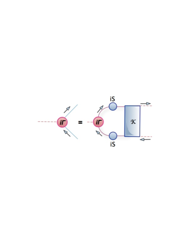
Figure 9: This diagram represents the BS equation. Blue (solid) circles represent dressed propagators $S$, red (solid) circle is the meson BSA $\Gamma$ and the blue (solid) rectangle is the dressed-quark-antiquark scattering kernel $K$.

The corresponding equation is Salpeter and Bethe (1951)

$$[\Gamma(k;P)]_{tu}=\int\!\frac{d^{4}q}{(2\pi)^{4}}[\chi(q;P)]_{sr}K_{tu}^{rs}(q,k;P)\,,$$ (C.21)

where $\Gamma$ is the bound-state’s BSA; $\chi(q;P)=S(q+P)\Gamma S(q)$ is the BS wave-function; $r,s,t,u$ represent colour, flavor and spinor indices; and $K$ is the relevant fermion-fermion scattering kernel. This equation possesses solutions on that discrete set of $P^{2}$-values for which bound-states exist.
A general decomposition of the bound-state’s BSA for scalar and axial-vector diquarks composed of quarks ${\color[rgb]{1,0,0}q}$ and ${\color[rgb]{0,0,1}q_{1}}$ in the CI model has the form :

$$\Gamma_{[{\color[rgb]{1,0,0}q}{\color[rgb]{0,0,1}q_{1}}]}^{0^{+}} = i\gamma_{5}E_{[{\color[rgb]{1,0,0}q}{\color[rgb]{0,0,1}q_{1}}]_{0^{+}}}+\frac{1}{2M_{R}}\gamma_{5}\gamma\cdot PF_{[{\color[rgb]{1,0,0}q}{\color[rgb]{0,0,1}q_{1}}]_{0^{+}}}\;,$$

$$\Gamma_{\{{\color[rgb]{1,0,0}q}{\color[rgb]{0,0,1}q_{1}}\},\mu}^{1^{+}} = \gamma_{\mu}^{T}E_{\{{\color[rgb]{1,0,0}q}{\color[rgb]{0,0,1}q_{1}}\}_{1^{+}}}+\frac{1}{2M_{R}}\sigma_{\mu\nu}P_{\nu}F_{\{{\color[rgb]{1,0,0}q}{\color[rgb]{0,0,1}q_{1}}\}_{1^{+}}}\;,$$ (C.22)

where $M_{R}=M_{{\color[rgb]{1,0,0}q}}M_{{\color[rgb]{0,0,1}q_{1}}}/[M_{{\color[rgb]{1,0,0}q}}+M_{{\color[rgb]{0,0,1}q_{1}}}]$ and $M_{{\color[rgb]{1,0,0}q}}$ and $M_{{\color[rgb]{0,0,1}q_{1}}}$ are the quark masses. The amplitudes in Eq. (C) are crucial for determining the masses listed in Table 1.

Appendix D Kernel in FE

In this section, we provide the explicit expressions for the elements of the matrix in the Eq. (LABEL:B-matrix),

$$\mathcal{M}^{11} =t^{{\color[rgb]{1,0,0}q}T}t^{[{\color[rgb]{1,0,0}q}{\color[rgb]{0,0,1}q_{1}}]}t^{[{\color[rgb]{1,0,0}q}{\color[rgb]{0,0,1}q_{1}}]T}t^{{\color[rgb]{1,0,0}q}}$$

$$\times\{{\color[rgb]{0,0,0}\Gamma}^{0^{+}}_{[{\color[rgb]{1,0,0}q}{\color[rgb]{0,0,1}q_{1}}]}(l_{{\color[rgb]{1,0,0}q}{\color[rgb]{0,0,1}q_{1}}})S_{{\color[rgb]{0,0,1}q_{1}}}^{T}\overline{{\color[rgb]{0,0,0}\Gamma}}^{0^{+}}_{[{\color[rgb]{1,0,0}q}{\color[rgb]{0,0,1}q_{1}}]}(-k_{{\color[rgb]{1,0,0}q}{\color[rgb]{0,0,1}q_{1}}})S_{{\color[rgb]{1,0,0}q}}(l_{{\color[rgb]{1,0,0}q}}){\color[rgb]{0,0,0}\Delta}^{0^{+}}_{[{\color[rgb]{1,0,0}q}{\color[rgb]{0,0,1}q_{1}}]}(l_{{\color[rgb]{1,0,0}q}{\color[rgb]{0,0,1}q_{1}}})\}\;,$$

$$\mathcal{M}^{12}_{\nu} =t^{{\color[rgb]{1,0,0}q}T}t^{\{{\color[rgb]{1,0,0}q}{\color[rgb]{1,0,0}q}\}}t^{[{\color[rgb]{1,0,0}q}{\color[rgb]{0,0,1}q_{1}}]T}t^{{\color[rgb]{0,0,1}q_{1}}}$$

$$\times\{{\color[rgb]{0,0,0}\Gamma}^{1^{+}}_{\{{\color[rgb]{1,0,0}q}{\color[rgb]{1,0,0}q}\},\mu}(l_{{\color[rgb]{1,0,0}q}{\color[rgb]{1,0,0}q}})S_{{\color[rgb]{1,0,0}q}}^{T}\overline{{\color[rgb]{0,0,0}\Gamma}}^{0^{+}}_{[{\color[rgb]{1,0,0}q}{\color[rgb]{0,0,1}q_{1}}]}(-k_{{\color[rgb]{1,0,0}q}{\color[rgb]{0,0,1}q_{1}}})S_{{\color[rgb]{0,0,1}q_{1}}}(l_{{\color[rgb]{0,0,1}q_{1}}}){\color[rgb]{0,0,0}\Delta}^{1^{+}}_{\{{\color[rgb]{1,0,0}q}{\color[rgb]{1,0,0}q}\},\mu\nu}(l_{{\color[rgb]{1,0,0}q}{\color[rgb]{1,0,0}q}})\}\;,$$

$$\mathcal{M}^{13}_{\nu} =t^{{\color[rgb]{1,0,0}q}T}t^{\{{\color[rgb]{1,0,0}q}{\color[rgb]{0,0,1}q_{1}}\}}t^{[{\color[rgb]{1,0,0}q}{\color[rgb]{0,0,1}q_{1}}]T}t^{{\color[rgb]{1,0,0}q}}$$

$$\times\{{\color[rgb]{0,0,0}\Gamma}^{1^{+}}_{\{{\color[rgb]{1,0,0}q}{\color[rgb]{0,0,1}q_{1}}\},\mu}(l_{{\color[rgb]{1,0,0}q}{\color[rgb]{0,0,1}q_{1}}})S_{{\color[rgb]{0,0,1}q_{1}}}^{T}\overline{{\color[rgb]{0,0,0}\Gamma}}^{0^{+}}_{[{\color[rgb]{1,0,0}q}{\color[rgb]{0,0,1}q_{1}}]}(-k_{{\color[rgb]{1,0,0}q}{\color[rgb]{0,0,1}q_{1}}})S_{{\color[rgb]{1,0,0}q}}(l_{{\color[rgb]{1,0,0}q}}){\color[rgb]{0,0,0}\Delta}^{1^{+}}_{\{{\color[rgb]{1,0,0}q}{\color[rgb]{0,0,1}q_{1}}\},\mu\nu}(l_{{\color[rgb]{1,0,0}q}{\color[rgb]{0,0,1}q_{1}}})\}\;,$$

$$\mathcal{M}^{14}_{\nu} =t^{{\color[rgb]{1,0,0}q}T}t^{\{{\color[rgb]{1,0,0}q}{\color[rgb]{1,0,0}q}\}}t^{[{\color[rgb]{1,0,0}q}{\color[rgb]{0,0,1}q_{1}}]T}t^{{\color[rgb]{0,0,1}q_{1}}}$$

$$\times{\color[rgb]{0,0,0}\Gamma}^{1^{+}}_{\{{\color[rgb]{1,0,0}q}{\color[rgb]{1,0,0}q}\},\mu}(l_{{\color[rgb]{1,0,0}q}{\color[rgb]{1,0,0}q}})S_{{\color[rgb]{1,0,0}q}}^{T}\overline{{\color[rgb]{0,0,0}\Gamma}}^{0^{+}}_{[{\color[rgb]{1,0,0}q}{\color[rgb]{0,0,1}q_{1}}]}(-k_{{\color[rgb]{1,0,0}q}{\color[rgb]{0,0,1}q_{1}}})S_{{\color[rgb]{0,0,1}q_{1}}}(l_{{\color[rgb]{0,0,1}q_{1}}}){\color[rgb]{0,0,0}\Delta}^{1^{+}}_{\{{\color[rgb]{1,0,0}q}{\color[rgb]{1,0,0}q}\},\mu\nu}(l_{{\color[rgb]{1,0,0}q}{\color[rgb]{1,0,0}q}})\}\;,$$

$$\mathcal{M}^{15}_{\nu} =t^{{\color[rgb]{1,0,0}q}T}t^{\{{\color[rgb]{1,0,0}q}{\color[rgb]{0,0,1}q_{1}}\}}t^{[{\color[rgb]{1,0,0}q}{\color[rgb]{0,0,1}q_{1}}]T}t^{{\color[rgb]{1,0,0}q}}$$

$$\times \{{\color[rgb]{0,0,0}\Gamma}^{1^{+}}_{\{{\color[rgb]{1,0,0}q}{\color[rgb]{0,0,1}q_{1}}\},\mu}(l_{{\color[rgb]{1,0,0}q}{\color[rgb]{0,0,1}q_{1}}})S_{{\color[rgb]{0,0,1}q_{1}}}^{T}\overline{{\color[rgb]{0,0,0}\Gamma}}^{0^{+}}_{[{\color[rgb]{1,0,0}q}{\color[rgb]{0,0,1}q_{1}}]}(-k_{{\color[rgb]{1,0,0}q}{\color[rgb]{0,0,1}q_{1}}})S_{{\color[rgb]{1,0,0}q}}(l_{{\color[rgb]{1,0,0}q}}){\color[rgb]{0,0,0}\Delta}^{1^{+}}_{\{{\color[rgb]{1,0,0}q}{\color[rgb]{0,0,1}q_{1}}\},\mu\nu}(l_{{\color[rgb]{1,0,0}q}{\color[rgb]{0,0,1}q_{1}}})\}\;,$$

$$\mathcal{M}^{21}_{\mu} =t^{{\color[rgb]{0,0,1}q_{1}}T}t^{[{\color[rgb]{1,0,0}q}{\color[rgb]{0,0,1}q_{1}}]}t^{\{{\color[rgb]{1,0,0}q}{\color[rgb]{1,0,0}q}\}T}t^{{\color[rgb]{1,0,0}q}}$$

$$\times \{\{{\color[rgb]{0,0,0}\Gamma}^{0^{+}}_{[{\color[rgb]{1,0,0}q}{\color[rgb]{0,0,1}q_{1}}]}(l_{{\color[rgb]{1,0,0}q}{\color[rgb]{0,0,1}q_{1}}})S_{{\color[rgb]{1,0,0}q}}^{T}\overline{{\color[rgb]{0,0,0}\Gamma}}^{1^{+}}_{\{{\color[rgb]{1,0,0}q}{\color[rgb]{1,0,0}q}\},\mu}(-k_{{\color[rgb]{1,0,0}q}{\color[rgb]{1,0,0}q}})S_{{\color[rgb]{1,0,0}q}}(l_{{\color[rgb]{1,0,0}q}}){\color[rgb]{0,0,0}\Delta}^{0^{+}}_{[{\color[rgb]{1,0,0}q}{\color[rgb]{0,0,1}q_{1}}]}(l_{{\color[rgb]{1,0,0}q}{\color[rgb]{0,0,1}q_{1}}})\}\;,$$

$$\mathcal{M}^{22}_{\mu\nu} =t^{{\color[rgb]{0,0,1}q_{1}}T}t^{\{{\color[rgb]{1,0,0}q}{\color[rgb]{1,0,0}q}\}}t^{\{{\color[rgb]{1,0,0}q}{\color[rgb]{1,0,0}q}\}T}t^{{\color[rgb]{0,0,1}q_{1}}}$$

$$\times \{{\color[rgb]{0,0,0}\Gamma}^{1^{+}}_{\{{\color[rgb]{1,0,0}q}{\color[rgb]{1,0,0}q}\},\rho}(l_{{\color[rgb]{1,0,0}q}{\color[rgb]{1,0,0}q}})S_{{\color[rgb]{0,0,1}q_{1}}}^{T}\overline{{\color[rgb]{0,0,0}\Gamma}}^{1^{+}}_{\{{\color[rgb]{1,0,0}q}{\color[rgb]{1,0,0}q}\},\mu}(-k_{{\color[rgb]{1,0,0}q}{\color[rgb]{1,0,0}q}})S_{{\color[rgb]{0,0,1}q_{1}}}(l_{{\color[rgb]{0,0,1}q_{1}}}){\color[rgb]{0,0,0}\Delta}^{1^{+}}_{\{{\color[rgb]{1,0,0}q}{\color[rgb]{1,0,0}q}\},\rho\nu}(l_{{\color[rgb]{1,0,0}q}{\color[rgb]{1,0,0}q}})\}\;,$$

$$\mathcal{M}^{23}_{\mu\nu} =t^{{\color[rgb]{0,0,1}q_{1}}T}t^{\{{\color[rgb]{1,0,0}q}{\color[rgb]{0,0,1}q_{1}}\}}t^{\{{\color[rgb]{1,0,0}q}{\color[rgb]{1,0,0}q}\}T}t^{{\color[rgb]{1,0,0}q}}$$

$$\times \{{\color[rgb]{0,0,0}\Gamma}^{1^{+}}_{\{{\color[rgb]{1,0,0}q}{\color[rgb]{0,0,1}q_{1}}\},\rho}(l_{{\color[rgb]{1,0,0}q}{\color[rgb]{0,0,1}q_{1}}})S_{{\color[rgb]{1,0,0}q}}^{T}\overline{{\color[rgb]{0,0,0}\Gamma}}^{1^{+}}_{\{{\color[rgb]{1,0,0}q}{\color[rgb]{1,0,0}q}\},\mu}(-k_{{\color[rgb]{1,0,0}q}{\color[rgb]{1,0,0}q}})S_{{\color[rgb]{1,0,0}q}}(l_{{\color[rgb]{1,0,0}q}}){\color[rgb]{0,0,0}\Delta}^{1^{+}}_{\{{\color[rgb]{1,0,0}q}{\color[rgb]{0,0,1}q_{1}}\},\rho\nu}(l_{{\color[rgb]{1,0,0}q}{\color[rgb]{0,0,1}q_{1}}})\}\;,$$

$$\mathcal{M}^{24}_{\mu\nu} =t^{{\color[rgb]{0,0,1}q_{1}}T}t^{\{{\color[rgb]{1,0,0}q}{\color[rgb]{1,0,0}q}\}}t^{\{{\color[rgb]{1,0,0}q}{\color[rgb]{1,0,0}q}\}T}t^{{\color[rgb]{0,0,1}q_{1}}}$$

$$\times \{{\color[rgb]{0,0,0}\Gamma}^{1^{+}}_{\{{\color[rgb]{1,0,0}q}{\color[rgb]{1,0,0}q}\},\rho}(l_{{\color[rgb]{1,0,0}q}{\color[rgb]{1,0,0}q}})S_{{\color[rgb]{0,0,1}q_{1}}}^{T}\overline{{\color[rgb]{0,0,0}\Gamma}}^{1^{+}}_{\{{\color[rgb]{1,0,0}q}{\color[rgb]{1,0,0}q}\},\mu}(-k_{{\color[rgb]{1,0,0}q}{\color[rgb]{1,0,0}q}})S_{{\color[rgb]{0,0,1}q_{1}}}(l_{{\color[rgb]{0,0,1}q_{1}}}){\color[rgb]{0,0,0}\Delta}^{1^{+}}_{\{{\color[rgb]{1,0,0}q}{\color[rgb]{1,0,0}q}\},\rho\nu}(l_{{\color[rgb]{1,0,0}q}{\color[rgb]{1,0,0}q}})\}\;,$$

$$\mathcal{M}^{25}_{\mu\nu} =t^{{\color[rgb]{0,0,1}q_{1}}T}t^{\{{\color[rgb]{1,0,0}q}{\color[rgb]{0,0,1}q_{1}}\}}t^{\{{\color[rgb]{1,0,0}q}{\color[rgb]{1,0,0}q}\}T}t^{{\color[rgb]{1,0,0}q}}$$

$$\times \{{\color[rgb]{0,0,0}\Gamma}^{1^{+}}_{\{{\color[rgb]{1,0,0}q}{\color[rgb]{0,0,1}q_{1}}\},\rho}(l_{{\color[rgb]{1,0,0}q}{\color[rgb]{0,0,1}q_{1}}})S_{{\color[rgb]{1,0,0}q}}^{T}\overline{{\color[rgb]{0,0,0}\Gamma}}^{1^{+}}_{\{{\color[rgb]{1,0,0}q}{\color[rgb]{1,0,0}q}\},\mu}(-k_{{\color[rgb]{1,0,0}q}{\color[rgb]{1,0,0}q}})S_{{\color[rgb]{1,0,0}q}}(l_{{\color[rgb]{1,0,0}q}}){\color[rgb]{0,0,0}\Delta}^{1^{+}}_{\{{\color[rgb]{1,0,0}q}{\color[rgb]{0,0,1}q_{1}}\},\rho\nu}(l_{{\color[rgb]{1,0,0}q}{\color[rgb]{0,0,1}q_{1}}})\}\;,$$

$$\mathcal{M}^{31}_{\mu}\ =t^{{\color[rgb]{1,0,0}q}T}t^{[{\color[rgb]{1,0,0}q}{\color[rgb]{0,0,1}q_{1}}]}t^{\{{\color[rgb]{1,0,0}q}{\color[rgb]{0,0,1}q_{1}}\}T}t^{{\color[rgb]{1,0,0}q}}$$

$$\times \{{\color[rgb]{0,0,0}\Gamma}^{0^{+}}_{[{\color[rgb]{1,0,0}q}{\color[rgb]{0,0,1}q_{1}}]}(l_{{\color[rgb]{1,0,0}q}{\color[rgb]{0,0,1}q_{1}}})S_{{\color[rgb]{0,0,1}q_{1}}}^{T}\overline{{\color[rgb]{0,0,0}\Gamma}}^{1^{+}}_{\{{\color[rgb]{1,0,0}q}{\color[rgb]{0,0,1}q_{1}}\},\mu}(-k_{{\color[rgb]{1,0,0}q}{\color[rgb]{0,0,1}q_{1}}})S_{{\color[rgb]{1,0,0}q}}(l_{{\color[rgb]{1,0,0}q}}){\color[rgb]{0,0,0}\Delta}^{0^{+}}_{[{\color[rgb]{1,0,0}q}{\color[rgb]{0,0,1}q_{1}}]}(l_{{\color[rgb]{1,0,0}q}{\color[rgb]{0,0,1}q_{1}}})\}\;,$$

$$\mathcal{M}^{32}_{\mu\nu} =t^{{\color[rgb]{1,0,0}q}T}t^{\{{\color[rgb]{1,0,0}q}{\color[rgb]{1,0,0}q}\}}t^{\{{\color[rgb]{1,0,0}q}{\color[rgb]{1,0,0}q}\}T}t^{{\color[rgb]{0,0,1}q_{1}}}$$

$$\times \{{\color[rgb]{0,0,0}\Gamma}^{1^{+}}_{\{{\color[rgb]{1,0,0}q}{\color[rgb]{1,0,0}q}\},\rho}(l_{{\color[rgb]{1,0,0}q}{\color[rgb]{1,0,0}q}})S_{{\color[rgb]{1,0,0}q}}^{T}\overline{{\color[rgb]{0,0,0}\Gamma}}^{1^{+}}_{\{{\color[rgb]{1,0,0}q}{\color[rgb]{0,0,1}q_{1}}\},\mu}(-k_{{\color[rgb]{1,0,0}q}{\color[rgb]{0,0,1}q_{1}}})S_{{\color[rgb]{0,0,1}q_{1}}}(l_{{\color[rgb]{0,0,1}q_{1}}}){\color[rgb]{0,0,0}\Delta}^{0^{+}}_{\{{\color[rgb]{1,0,0}q}{\color[rgb]{1,0,0}q}\},\rho\nu}(l_{{\color[rgb]{1,0,0}q}{\color[rgb]{1,0,0}q}})\}\;,$$

$$\mathcal{M}^{33}_{\mu\nu} =t^{{\color[rgb]{1,0,0}q}T}t^{\{{\color[rgb]{1,0,0}q}{\color[rgb]{0,0,1}q_{1}}\}}t^{\{{\color[rgb]{1,0,0}q}{\color[rgb]{0,0,1}q_{1}}\}T}t^{{\color[rgb]{1,0,0}q}}$$

$$\times \{{\color[rgb]{0,0,0}\Gamma}^{1^{+}}_{\{{\color[rgb]{1,0,0}q}{\color[rgb]{0,0,1}q_{1}}\},\rho}(l_{{\color[rgb]{1,0,0}q}{\color[rgb]{0,0,1}q_{1}}})S_{{\color[rgb]{1,0,0}q}}^{T}\overline{{\color[rgb]{0,0,0}\Gamma}}^{1^{+}}_{\{{\color[rgb]{1,0,0}q}{\color[rgb]{0,0,1}q_{1}}\},\mu}(-k_{{\color[rgb]{1,0,0}q}{\color[rgb]{0,0,1}q_{1}}})S_{{\color[rgb]{1,0,0}q}}(l_{{\color[rgb]{1,0,0}q}}){\color[rgb]{0,0,0}\Delta}^{0^{+}}_{\{{\color[rgb]{1,0,0}q}{\color[rgb]{0,0,1}q_{1}}\},\rho\nu}(l_{{\color[rgb]{1,0,0}q}{\color[rgb]{0,0,1}q_{1}}})\}\;,$$

$$\mathcal{M}^{34}_{\mu\nu} =t^{{\color[rgb]{1,0,0}q}T}t^{\{{\color[rgb]{1,0,0}q}{\color[rgb]{1,0,0}q}\}}t^{\{{\color[rgb]{1,0,0}q}{\color[rgb]{1,0,0}q}\}T}t^{{\color[rgb]{0,0,1}q_{1}}}$$

$$\times \{{\color[rgb]{0,0,0}\Gamma}^{1^{+}}_{\{{\color[rgb]{1,0,0}q}{\color[rgb]{1,0,0}q}\},\rho}(l_{{\color[rgb]{1,0,0}q}{\color[rgb]{1,0,0}q}})S_{{\color[rgb]{1,0,0}q}}^{T}\overline{{\color[rgb]{0,0,0}\Gamma}}^{1^{+}}_{\{{\color[rgb]{1,0,0}q}{\color[rgb]{0,0,1}q_{1}}\},\mu}(-k_{{\color[rgb]{1,0,0}q}{\color[rgb]{0,0,1}q_{1}}})S_{{\color[rgb]{0,0,1}q_{1}}}(l_{{\color[rgb]{0,0,1}q_{1}}}){\color[rgb]{0,0,0}\Delta}^{0^{+}}_{\{{\color[rgb]{1,0,0}q}{\color[rgb]{1,0,0}q}\},\rho\nu}(l_{{\color[rgb]{1,0,0}q}{\color[rgb]{1,0,0}q}})\}\;,$$

$$\mathcal{M}^{35}_{\mu\nu} =t^{{\color[rgb]{1,0,0}q}T}t^{\{{\color[rgb]{1,0,0}q}{\color[rgb]{0,0,1}q_{1}}\}}t^{\{{\color[rgb]{1,0,0}q}{\color[rgb]{0,0,1}q_{1}}\}T}t^{{\color[rgb]{1,0,0}q}}$$

$$\times \{{\color[rgb]{0,0,0}\Gamma}^{1^{+}}_{\{{\color[rgb]{1,0,0}q}{\color[rgb]{0,0,1}q_{1}}\},\rho}(l_{{\color[rgb]{1,0,0}q}{\color[rgb]{0,0,1}q_{1}}})S_{{\color[rgb]{1,0,0}q}}^{T}\overline{{\color[rgb]{0,0,0}\Gamma}}^{1^{+}}_{\{{\color[rgb]{1,0,0}q}{\color[rgb]{0,0,1}q_{1}}\},\mu}(-k_{{\color[rgb]{1,0,0}q}{\color[rgb]{0,0,1}q_{1}}})S_{{\color[rgb]{1,0,0}q}}(l_{{\color[rgb]{1,0,0}q}}){\color[rgb]{0,0,0}\Delta}^{0^{+}}_{\{{\color[rgb]{1,0,0}q}{\color[rgb]{0,0,1}q_{1}}\},\rho\nu}(l_{{\color[rgb]{1,0,0}q}{\color[rgb]{0,0,1}q_{1}}})\}\;,$$

$$\mathcal{M}^{41}_{\mu} =t^{{\color[rgb]{0,0,1}q_{1}}T}t^{[{\color[rgb]{1,0,0}q}{\color[rgb]{0,0,1}q_{1}}]}t^{\{{\color[rgb]{1,0,0}q}{\color[rgb]{1,0,0}q}\}T}t^{{\color[rgb]{1,0,0}q}}$$

$$\times \{\{{\color[rgb]{0,0,0}\Gamma}^{0^{+}}_{[{\color[rgb]{1,0,0}q}{\color[rgb]{0,0,1}q_{1}}]}(l_{{\color[rgb]{1,0,0}q}{\color[rgb]{0,0,1}q_{1}}})S_{{\color[rgb]{1,0,0}q}}^{T}\overline{{\color[rgb]{0,0,0}\Gamma}}^{1^{+}}_{\{{\color[rgb]{1,0,0}q}{\color[rgb]{1,0,0}q}\},\mu}(-k_{{\color[rgb]{1,0,0}q}{\color[rgb]{1,0,0}q}})S_{{\color[rgb]{1,0,0}q}}(l_{{\color[rgb]{1,0,0}q}}){\color[rgb]{0,0,0}\Delta}^{0^{+}}_{[{\color[rgb]{1,0,0}q}{\color[rgb]{0,0,1}q_{1}}]}(l_{{\color[rgb]{1,0,0}q}{\color[rgb]{0,0,1}q_{1}}})\}\;,$$

$$\mathcal{M}^{42}_{\mu\nu} =t^{{\color[rgb]{0,0,1}q_{1}}T}t^{\{{\color[rgb]{1,0,0}q}{\color[rgb]{1,0,0}q}\}}t^{\{{\color[rgb]{1,0,0}q}{\color[rgb]{1,0,0}q}\}T}t^{{\color[rgb]{0,0,1}q_{1}}}$$

$$\times \{{\color[rgb]{0,0,0}\Gamma}^{1^{+}}_{\{{\color[rgb]{1,0,0}q}{\color[rgb]{1,0,0}q}\},\rho}(l_{{\color[rgb]{1,0,0}q}{\color[rgb]{1,0,0}q}})S_{{\color[rgb]{0,0,1}q_{1}}}^{T}\overline{{\color[rgb]{0,0,0}\Gamma}}^{1^{+}}_{\{{\color[rgb]{1,0,0}q}{\color[rgb]{1,0,0}q}\},\mu}(-k_{{\color[rgb]{1,0,0}q}{\color[rgb]{1,0,0}q}})S_{{\color[rgb]{0,0,1}q_{1}}}(l_{{\color[rgb]{0,0,1}q_{1}}}){\color[rgb]{0,0,0}\Delta}^{1^{+}}_{\{{\color[rgb]{1,0,0}q}{\color[rgb]{1,0,0}q}\},\rho\nu}(l_{{\color[rgb]{1,0,0}q}{\color[rgb]{1,0,0}q}})\}\;,$$

$$\mathcal{M}^{43}_{\mu\nu} =t^{{\color[rgb]{0,0,1}q_{1}}T}t^{\{{\color[rgb]{1,0,0}q}{\color[rgb]{0,0,1}q_{1}}\}}t^{\{{\color[rgb]{1,0,0}q}{\color[rgb]{1,0,0}q}\}T}t^{{\color[rgb]{1,0,0}q}}$$

$$\times\{{\color[rgb]{0,0,0}\Gamma}^{1^{+}}_{\{{\color[rgb]{1,0,0}q}{\color[rgb]{0,0,1}q_{1}}\},\rho}(l_{{\color[rgb]{1,0,0}q}{\color[rgb]{1,0,0}q}})S_{{\color[rgb]{1,0,0}q}}^{T}\overline{{\color[rgb]{0,0,0}\Gamma}}^{1^{+}}_{\{{\color[rgb]{1,0,0}q}{\color[rgb]{1,0,0}q}\},\mu}(-k_{{\color[rgb]{1,0,0}q}{\color[rgb]{1,0,0}q}})S_{{\color[rgb]{1,0,0}q}}(l_{{\color[rgb]{1,0,0}q}}){\color[rgb]{0,0,0}\Delta}^{1^{+}}_{\{{\color[rgb]{1,0,0}q}{\color[rgb]{0,0,1}q_{1}}\},\rho\nu}(l_{{\color[rgb]{1,0,0}q}{\color[rgb]{0,0,1}q_{1}}})\}\;,$$

$$\mathcal{M}^{44}_{\mu\nu} =t^{{\color[rgb]{0,0,1}q_{1}}T}t^{\{{\color[rgb]{1,0,0}q}{\color[rgb]{1,0,0}q}\}}t^{\{{\color[rgb]{1,0,0}q}{\color[rgb]{1,0,0}q}\}T}t^{{\color[rgb]{0,0,1}q_{1}}}$$

$$\times \{{\color[rgb]{0,0,0}\Gamma}^{1^{+}}_{\{{\color[rgb]{1,0,0}q}{\color[rgb]{1,0,0}q}\},\rho}(l_{{\color[rgb]{1,0,0}q}{\color[rgb]{1,0,0}q}})S_{{\color[rgb]{0,0,1}q_{1}}}^{T}\overline{{\color[rgb]{0,0,0}\Gamma}}^{1^{+}}_{\{{\color[rgb]{1,0,0}q}{\color[rgb]{1,0,0}q}\},\mu}(-k_{{\color[rgb]{1,0,0}q}{\color[rgb]{1,0,0}q}})S_{{\color[rgb]{0,0,1}q_{1}}}(l_{{\color[rgb]{0,0,1}q_{1}}}){\color[rgb]{0,0,0}\Delta}^{1^{+}}_{\{{\color[rgb]{1,0,0}q}{\color[rgb]{1,0,0}q}\},\rho\nu}(l_{{\color[rgb]{1,0,0}q}{\color[rgb]{1,0,0}q}})\}\;,$$

$$\mathcal{M}^{45}_{\mu\nu} =t^{{\color[rgb]{0,0,1}q_{1}}T}t^{\{{\color[rgb]{1,0,0}q}{\color[rgb]{0,0,1}q_{1}}\}}t^{\{{\color[rgb]{1,0,0}q}{\color[rgb]{1,0,0}q}\}T}t^{{\color[rgb]{1,0,0}q}}$$

$$\times \{{\color[rgb]{0,0,0}\Gamma}^{1^{+}}_{\{{\color[rgb]{1,0,0}q}{\color[rgb]{0,0,1}q_{1}}\},\rho}(l_{{\color[rgb]{1,0,0}q}{\color[rgb]{0,0,1}q_{1}}})S_{{\color[rgb]{1,0,0}q}}^{T}\overline{{\color[rgb]{0,0,0}\Gamma}}^{1^{+}}_{\{{\color[rgb]{1,0,0}q}{\color[rgb]{1,0,0}q}\},\mu}(-k_{{\color[rgb]{1,0,0}q}{\color[rgb]{1,0,0}q}})S_{{\color[rgb]{1,0,0}q}}(l_{{\color[rgb]{0,0,1}q_{1}}}){\color[rgb]{0,0,0}\Delta}^{1^{+}}_{\{{\color[rgb]{1,0,0}q}{\color[rgb]{0,0,1}q_{1}}\},\rho\nu}(l_{{\color[rgb]{1,0,0}q}{\color[rgb]{0,0,1}q_{1}}})\}\;,$$

$$\mathcal{M}^{51}_{\mu} =t^{{\color[rgb]{1,0,0}q}T}t^{[{\color[rgb]{1,0,0}q}{\color[rgb]{0,0,1}q_{1}}]}t^{\{{\color[rgb]{1,0,0}q}{\color[rgb]{0,0,1}q_{1}}\}T}t^{{\color[rgb]{1,0,0}q}}$$

$$\times \{{\color[rgb]{0,0,0}\Gamma}^{0^{+}}_{[{\color[rgb]{1,0,0}q}{\color[rgb]{0,0,1}q_{1}}]}(l_{{\color[rgb]{1,0,0}q}{\color[rgb]{0,0,1}q_{1}}})S_{{\color[rgb]{0,0,1}q_{1}}}^{T}\overline{{\color[rgb]{0,0,0}\Gamma}}^{1^{+}}_{\{{\color[rgb]{1,0,0}q}{\color[rgb]{0,0,1}q_{1}}\},\mu}(-k_{{\color[rgb]{1,0,0}q}{\color[rgb]{0,0,1}q_{1}}})S_{{\color[rgb]{1,0,0}q}}(l_{{\color[rgb]{1,0,0}q}}){\color[rgb]{0,0,0}\Delta}^{0^{+}}_{[{\color[rgb]{1,0,0}q}{\color[rgb]{0,0,1}q_{1}}]}(l_{{\color[rgb]{1,0,0}q}{\color[rgb]{0,0,1}q_{1}}})\}\;,$$

$$\mathcal{M}^{52}_{\mu\nu} =t^{{\color[rgb]{1,0,0}q}T}t^{\{{\color[rgb]{1,0,0}q}{\color[rgb]{1,0,0}q}\}}t^{\{{\color[rgb]{1,0,0}q}{\color[rgb]{1,0,0}q}\}T}t^{{\color[rgb]{0,0,1}q_{1}}}$$

$$\times \{{\color[rgb]{0,0,0}\Gamma}^{1^{+}}_{\{{\color[rgb]{1,0,0}q}{\color[rgb]{1,0,0}q}\},\rho}(l_{{\color[rgb]{1,0,0}q}{\color[rgb]{1,0,0}q}})S_{{\color[rgb]{1,0,0}q}}^{T}\overline{{\color[rgb]{0,0,0}\Gamma}}^{1^{+}}_{\{{\color[rgb]{1,0,0}q}{\color[rgb]{0,0,1}q_{1}}\},\mu}(-k_{{\color[rgb]{1,0,0}q}{\color[rgb]{0,0,1}q_{1}}})S_{{\color[rgb]{0,0,1}q_{1}}}(l_{{\color[rgb]{0,0,1}q_{1}}}){\color[rgb]{0,0,0}\Delta}^{0^{+}}_{\{{\color[rgb]{1,0,0}q}{\color[rgb]{1,0,0}q}\},\rho\nu}(l_{{\color[rgb]{1,0,0}q}{\color[rgb]{1,0,0}q}})\}\;,$$

$$\mathcal{M}^{53}_{\mu\nu} =t^{{\color[rgb]{1,0,0}q}T}t^{\{{\color[rgb]{1,0,0}q}{\color[rgb]{0,0,1}q_{1}}\}}t^{\{{\color[rgb]{1,0,0}q}{\color[rgb]{0,0,1}q_{1}}\}T}t^{{\color[rgb]{1,0,0}q}}$$

$$\times \{{\color[rgb]{0,0,0}\Gamma}^{1^{+}}_{\{{\color[rgb]{1,0,0}q}{\color[rgb]{0,0,1}q_{1}}\},\rho}(l_{{\color[rgb]{1,0,0}q}{\color[rgb]{0,0,1}q_{1}}})S_{{\color[rgb]{1,0,0}q}}^{T}\overline{{\color[rgb]{0,0,0}\Gamma}}^{1^{+}}_{\{{\color[rgb]{1,0,0}q}{\color[rgb]{0,0,1}q_{1}}\},\mu}(-k_{{\color[rgb]{1,0,0}q}{\color[rgb]{0,0,1}q_{1}}})S_{{\color[rgb]{1,0,0}q}}(l_{{\color[rgb]{1,0,0}q}}){\color[rgb]{0,0,0}\Delta}^{0^{+}}_{\{{\color[rgb]{1,0,0}q}{\color[rgb]{0,0,1}q_{1}}\},\rho\nu}(l_{{\color[rgb]{1,0,0}q}{\color[rgb]{0,0,1}q_{1}}})\}\;,$$

$$\mathcal{M}^{54}_{\mu\nu} =t^{{\color[rgb]{1,0,0}q}T}t^{\{{\color[rgb]{1,0,0}q}{\color[rgb]{1,0,0}q}\}}t^{\{{\color[rgb]{1,0,0}q}{\color[rgb]{1,0,0}q}\}T}t^{{\color[rgb]{0,0,1}q_{1}}}$$

$$\times \{{\color[rgb]{0,0,0}\Gamma}^{1^{+}}_{\{{\color[rgb]{1,0,0}q}{\color[rgb]{1,0,0}q}\},\rho}(l_{{\color[rgb]{1,0,0}q}{\color[rgb]{1,0,0}q}})S_{{\color[rgb]{1,0,0}q}}^{T}\overline{{\color[rgb]{0,0,0}\Gamma}}^{1^{+}}_{\{{\color[rgb]{1,0,0}q}{\color[rgb]{0,0,1}q_{1}}\},\mu}(-k_{{\color[rgb]{1,0,0}q}{\color[rgb]{0,0,1}q_{1}}})S_{{\color[rgb]{0,0,1}q_{1}}}(l_{{\color[rgb]{0,0,1}q_{1}}}){\color[rgb]{0,0,0}\Delta}^{0^{+}}_{\{{\color[rgb]{1,0,0}q}{\color[rgb]{1,0,0}q}\},\rho\nu}(l_{{\color[rgb]{1,0,0}q}{\color[rgb]{1,0,0}q}})\}\;,$$

$$\mathcal{M}^{55}_{\mu\nu} =t^{{\color[rgb]{1,0,0}q}T}t^{\{{\color[rgb]{1,0,0}q}{\color[rgb]{0,0,1}q_{1}}\}}t^{\{{\color[rgb]{1,0,0}q}{\color[rgb]{0,0,1}q_{1}}\}T}t^{{\color[rgb]{1,0,0}q}}$$

$$\times \{{\color[rgb]{0,0,0}\Gamma}^{1^{+}}_{\{{\color[rgb]{1,0,0}q}{\color[rgb]{0,0,1}q_{1}}\},\rho}(l_{{\color[rgb]{1,0,0}q}{\color[rgb]{0,0,1}q_{1}}})S_{{\color[rgb]{1,0,0}q}}^{T}\overline{{\color[rgb]{0,0,0}\Gamma}}^{1^{+}}_{\{{\color[rgb]{1,0,0}q}{\color[rgb]{0,0,1}q_{1}}\},\mu}(-k_{{\color[rgb]{1,0,0}q}{\color[rgb]{0,0,1}q_{1}}})S_{{\color[rgb]{1,0,0}q}}(l_{{\color[rgb]{1,0,0}q}}){\color[rgb]{0,0,0}\Delta}^{0^{+}}_{\{{\color[rgb]{1,0,0}q}{\color[rgb]{0,0,1}q_{1}}\},\rho\nu}(l_{{\color[rgb]{1,0,0}q}{\color[rgb]{0,0,1}q_{1}}})\}\;.$$

$\Delta_{[{\color[rgb]{1,0,0}q}{\color[rgb]{0,0,1}q_{1}}]}^{0^{+}}(K)$ and $\Delta_{\{{\color[rgb]{1,0,0}q}{\color[rgb]{0,0,1}q_{1}}\},\mu\nu}^{1^{+}}(K)$, are standard propagators for scalar and vector diquarks.

$$\Delta_{[{\color[rgb]{1,0,0}q}{\color[rgb]{0,0,1}q_{1}}]}^{0^{+}}(K)=\frac{1}{K^{2}\!+\!m_{{\color[rgb]{1,0,0}q}{\color[rgb]{0,0,1}q_{1}}}^{2}},$$ (D.1)

$$\Delta_{\{{\color[rgb]{1,0,0}q}{\color[rgb]{0,0,1}q_{1}}\},\mu\nu}^{1^{+}}(K)\!=\!\frac{1}{K^{2}+m_{{\color[rgb]{1,0,0}q}{\color[rgb]{0,0,1}q_{1}}}^{2}}\left(\!\delta_{\mu\nu}\!+\!\frac{K_{\mu}K_{\nu}}{m_{{\color[rgb]{1,0,0}q}{\color[rgb]{0,0,1}q_{1}}}^{2}}\!\right).$$ (D.2)

With these expressions, the calculation of the baryonic masses with spin $1/2$ in Section II is straightforward.

Appendix E Flavor Diquarks

We define the following set of flavor column matrices,

$$t^{{\color[rgb]{1,0,0}u}}=\begin{pmatrix}1\\ 0\\ 0\\ 0\\ 0\end{pmatrix},\;\;\;\;t^{{\color[rgb]{0.64,0.0,0.0}d}}=\begin{pmatrix}0\\ 1\\ 0\\ 0\\ 0\end{pmatrix},\;\;\;\;t^{{\color[rgb]{0,0.5,0}s}}=\begin{pmatrix}0\\ 0\\ 1\\ 0\\ 0\end{pmatrix},\;\;\;\;$$

$$t^{{\color[rgb]{0.55,0.0,0.55}c}}=\begin{pmatrix}0\\ 0\\ 0\\ 1\\ 0\end{pmatrix},\;\;\;\;t^{{\color[rgb]{0,0,1}b}}=\begin{pmatrix}0\\ 0\\ 0\\ 0\\ 1\end{pmatrix},\;\;\;\;$$ (E.3)

and

$$t^{f}=\left[\begin{matrix}t^{{\color[rgb]{1,0,0}q}T}t^{\{{\color[rgb]{0,0,1}q_{1}}{\color[rgb]{1,0,0}q}\}}t^{\{{\color[rgb]{0,0,1}q_{1}}{\color[rgb]{1,0,0}q}\}T}t^{{\color[rgb]{1,0,0}q}}&&t^{{\color[rgb]{1,0,0}q}T}t^{\{{\color[rgb]{1,0,0}q}{\color[rgb]{1,0,0}q}\}}t^{\{{\color[rgb]{0,0,1}q_{1}}{\color[rgb]{1,0,0}q}\}T}t^{{\color[rgb]{0,0,1}q_{1}}}\\ \\ t^{{\color[rgb]{0,0,1}q_{1}}T}t^{\{{\color[rgb]{0,0,1}q_{1}}{\color[rgb]{1,0,0}q}\}}t^{\{{\color[rgb]{1,0,0}q}{\color[rgb]{1,0,0}q}\}T}t^{{\color[rgb]{1,0,0}q}}&&t^{{\color[rgb]{0,0,1}q_{1}}T}t^{\{{\color[rgb]{1,0,0}q}{\color[rgb]{1,0,0}q}\}}t^{\{{\color[rgb]{1,0,0}q}{\color[rgb]{1,0,0}q}\}T}t^{{\color[rgb]{0,0,1}q_{1}}}\end{matrix}\right]\,.$$

The flavor matrices for the diquarks are

$$\begin{array}[]{cc}\bf{t^{[{\color[rgb]{1,0,0}u}{\color[rgb]{0.64,0.0,0.0}d}]}=\begin{pmatrix}0&1&0&0&0\\ -1&0&0&0&0\\ 0&0&0&0&0\\ 0&0&0&0&0\\ 0&0&0&0&0\end{pmatrix}}&\bf{t^{[{\color[rgb]{1,0,0}u}{\color[rgb]{0,0.5,0}s}]}=\begin{pmatrix}0&0&1&0&0\\ 0&0&0&0&0\\ -1&0&0&0&0\\ 0&0&0&0&0\\ 0&0&0&0&0\end{pmatrix}}\\[51.6665pt] \bf{t^{[{\color[rgb]{0.64,0.0,0.0}d}{\color[rgb]{0,0.5,0}s}]}=\begin{pmatrix}0&0&0&0&0\\ 0&0&1&0&0\\ 0&-1&0&0&0\\ 0&0&0&0&0\\ 0&0&0&0&0\end{pmatrix}}&\bf{t^{[{\color[rgb]{1,0,0}u}{\color[rgb]{0.55,0.0,0.55}c}]}=\begin{pmatrix}0&0&0&1&0\\ 0&0&0&0&0\\ 0&0&0&0&0\\ -1&0&0&0&0\\ 0&0&0&0&0\end{pmatrix}},\end{array}$$

$$\begin{array}[]{cc}\bf{t^{\{{\color[rgb]{1,0,0}u}{\color[rgb]{1,0,0}u}\}}=\begin{pmatrix}\sqrt{2}&0&0&0&0\\ 0&0&0&0&0\\ 0&0&0&0&0\\ 0&0&0&0&0\\ 0&0&0&0&0\end{pmatrix}}&\bf{t^{\{{\color[rgb]{1,0,0}u}{\color[rgb]{0.64,0.0,0.0}d}\}}=\begin{pmatrix}0&1&0&0&0\\ 1&0&0&0&0\\ 0&0&0&0&0\\ 0&0&0&0&0\\ 0&0&0&0&0\end{pmatrix}},\\[43.05542pt] \bf{t^{\{{\color[rgb]{1,0,0}u}{\color[rgb]{0,0.5,0}s}\}}=\begin{pmatrix}0&0&1&0&0\\ 0&0&0&0&0\\ 1&0&0&0&0\\ 0&0&0&0&0\\ 0&0&0&0&0\end{pmatrix}}&t^{\{{\color[rgb]{1,0,0}u}{\color[rgb]{0.55,0.0,0.55}c}\}}=\begin{pmatrix}0&0&0&1&0\\ 0&0&0&0&0\\ 0&0&0&0&0\\ 1&0&0&0&0\\ 0&0&0&0&0\end{pmatrix},\\[43.05542pt] \bf{t^{\{{\color[rgb]{0.64,0.0,0.0}d}{\color[rgb]{0.64,0.0,0.0}d}\}}=\begin{pmatrix}0&0&0&0&0\\ 0&\sqrt{2}&0&0&0\\ 0&0&0&0&0\\ 0&0&0&0&0\\ 0&0&0&0&0\end{pmatrix}}&\bf{t^{\{{\color[rgb]{0.64,0.0,0.0}d}{\color[rgb]{0,0.5,0}s}\}}}=\begin{pmatrix}0&0&0&0&0\\ 0&0&1&0&0\\ 0&1&0&0&0\\ 0&0&0&0&0\\ 0&0&0&0&0\end{pmatrix},\\[43.05542pt] \bf{t^{\{{\color[rgb]{0,0.5,0}s}{\color[rgb]{0,0.5,0}s}\}}=\begin{pmatrix}0&0&0&0&0\\ 0&0&0&0&0\\ 0&0&\sqrt{2}&0&0\\ 0&0&0&0&0\\ 0&0&0&0&0\end{pmatrix}},&t^{\{{\color[rgb]{0.55,0.0,0.55}c}{\color[rgb]{0.55,0.0,0.55}c}\}}=\begin{pmatrix}0&0&0&0&0\\ 0&0&0&0&0\\ 0&0&0&0&0\\ 0&0&0&\sqrt{2}&0\\ 0&0&0&0&0\end{pmatrix}\,,\\[43.05542pt] \bf{t^{[{\color[rgb]{0.64,0.0,0.0}d}{\color[rgb]{0.55,0.0,0.55}c}]}}=\begin{pmatrix}0&0&0&0&0\\ 0&0&0&1&0\\ 0&0&0&0&0\\ 0&-1&0&0&0\\ 0&0&0&0&0\end{pmatrix},&\bf{t^{[{\color[rgb]{0,0.5,0}s}{\color[rgb]{0.55,0.0,0.55}c}]}}=\begin{pmatrix}0&0&0&0&0\\ 0&0&0&0&0\\ 0&0&0&1&0\\ 0&0&-1&0&0\\ 0&0&0&0&0\end{pmatrix},\\[43.05542pt] \bf{t^{\{{\color[rgb]{0.64,0.0,0.0}d}{\color[rgb]{0.55,0.0,0.55}c}\}}}=\begin{pmatrix}0&0&0&0&0\\ 0&0&0&1&0\\ 0&0&0&0&0\\ 0&1&0&0&0\\ 0&0&0&0&0\end{pmatrix},&\bf{t^{\{{\color[rgb]{0,0.5,0}s}{\color[rgb]{0.55,0.0,0.55}c}\}}}=\begin{pmatrix}0&0&0&0&0\\ 0&0&0&0&0\\ 0&0&0&1&0\\ 0&0&1&0&0\\ 0&0&0&0&0\end{pmatrix},\\[43.05542pt] \bf{t^{[{\color[rgb]{0,0,1}b}{\color[rgb]{1,0,0}u}]}}=\begin{pmatrix}0&0&0&0&-1\\ 0&0&0&0&0\\ 0&0&0&0&0\\ 0&0&0&0&0\\ 1&0&0&0&0\end{pmatrix},&\bf{t^{[{\color[rgb]{0,0,1}b}{\color[rgb]{0.64,0.0,0.0}d}]}}=\begin{pmatrix}0&0&0&0&0\\ 0&0&0&0&-1\\ 0&0&0&0&0\\ 0&0&0&0&0\\ 0&1&0&0&0\end{pmatrix},\\[43.05542pt] \bf{t^{[{\color[rgb]{0,0,1}b}{\color[rgb]{0.55,0.0,0.55}c}]}}=\begin{pmatrix}0&0&0&0&0\\ 0&0&0&0&0\\ 0&0&0&0&0\\ 0&0&0&0&-1\\ 0&0&0&1&0\end{pmatrix},&\bf{t^{[{\color[rgb]{0,0,1}b}{\color[rgb]{0,0.5,0}s}]}}=\begin{pmatrix}0&0&0&0&0\\ 0&0&0&0&0\\ 0&0&0&0&-1\\ 0&0&0&0&0\\ 0&0&1&0&0\end{pmatrix},\\[43.05542pt] \bf{t^{\{{\color[rgb]{0,0,1}b}{\color[rgb]{0,0,1}b}\}}}=\begin{pmatrix}0&0&0&0&0\\ 0&0&0&0&0\\ 0&0&0&0&0\\ 0&0&0&0&0\\ 0&0&0&0&\sqrt{2}\end{pmatrix}&\bf{t^{\{{\color[rgb]{0,0,1}b}{\color[rgb]{1,0,0}u}\}}}=\begin{pmatrix}0&0&0&0&1\\ 0&0&0&0&0\\ 0&0&0&0&0\\ 0&0&0&0&0\\ 1&0&0&0&0\end{pmatrix},\end{array}$$

$$\begin{array}[]{cc}\bf{t^{\{{\color[rgb]{0,0,1}b}{\color[rgb]{0.64,0.0,0.0}d}\}}}=\begin{pmatrix}0&0&0&0&0\\ 0&0&0&0&1\\ 0&0&0&0&0\\ 0&0&0&0&0\\ 0&1&0&0&0\end{pmatrix}&\bf{t^{\{{\color[rgb]{0,0,1}b}{\color[rgb]{0.55,0.0,0.55}c}\}}}=\begin{pmatrix}0&0&0&0&0\\ 0&0&0&0&0\\ 0&0&0&0&0\\ 0&0&0&0&1\\ 0&0&0&1&0\end{pmatrix},\\[43.05542pt] \bf{t^{\{{\color[rgb]{0,0,1}b}{\color[rgb]{0,0.5,0}s}\}}}=\begin{pmatrix}0&0&0&0&0\\ 0&0&0&0&0\\ 0&0&0&0&1\\ 0&0&0&0&0\\ 0&0&1&0&0&\end{pmatrix}\end{array}$$

References

- Faddeev (1960) L. D. Faddeev, Zh. Eksp. Teor. Fiz. 39, 1459 (1960).
- Eichmann (2011) G. Eichmann, Phys. Rev. D 84, 014014 (2011), eprint 1104.4505.
- Eichmann et al. (2016) G. Eichmann, H. Sanchis-Alepuz, R. Williams, R. Alkofer, and C. S. Fischer, Prog. Part. Nucl. Phys. 91, 1 (2016), eprint 1606.09602.
- Gell-Mann (1964) M. Gell-Mann, Phys. Lett. 8, 214 (1964).
- Ida and Kobayashi (1966) M. Ida and R. Kobayashi, Prog. Theor. Phys. 36, 846 (1966).
- Lichtenberg and Tassie (1967) D. B. Lichtenberg and L. J. Tassie, Phys. Rev. 155, 1601 (1967).
- Lichtenberg (1969) D. B. Lichtenberg, Phys. Rev. 178, 2197 (1969).
- Barabanov et al. (2021) M. Y. Barabanov et al., Prog. Part. Nucl. Phys. 116, 103835 (2021), eprint 2008.07630.
- Wilczek (2004) F. Wilczek, in Deserfest: A Celebration of the Life and Works of Stanley Deser (2004), pp. 322–338, eprint hep-ph/0409168.
- Qin et al. (2019) S.-x. Qin, C. D. Roberts, and S. M. Schmidt, Few Body Syst. 60, 26 (2019), eprint 1902.00026.
- Ebert et al. (2002) D. Ebert, R. N. Faustov, V. O. Galkin, and A. P. Martynenko, Phys. Rev. D 66, 014008 (2002), eprint hep-ph/0201217.
- Yoshida et al. (2015) T. Yoshida, E. Hiyama, A. Hosaka, M. Oka, and K. Sadato, Phys. Rev. D 92, 114029 (2015), eprint 1510.01067.
- Giannuzzi (2009) F. Giannuzzi, Phys. Rev. D 79, 094002 (2009), eprint 0902.4624.
- Shah and Rai (2017a) Z. Shah and A. K. Rai, Eur. Phys. J. C 77, 129 (2017a), eprint 1702.02726.
- Shah et al. (2016) Z. Shah, K. Thakkar, and A. K. Rai, Eur. Phys. J. C 76, 530 (2016), eprint 1609.03030.
- Vishwakarma and Upadhyay (2022) K. K. Vishwakarma and A. Upadhyay (2022), eprint 2208.02536.
- Valcarce et al. (2008) A. Valcarce, H. Garcilazo, and J. Vijande, Eur. Phys. J. A 37, 217 (2008), eprint 0807.2973.
- Shekari Tousi and Azizi (2024) M. Shekari Tousi and K. Azizi, Phys. Rev. D 109, 054005 (2024), eprint 2401.07151.
- Alrebdi et al. (2022) H. I. Alrebdi, R. F. Alnahdi, and T. Barakat, Eur. Phys. J. C 82, 450 (2022).
- Alomayrah and Barakat (2020) N. Alomayrah and T. Barakat, Eur. Phys. J. A 56, 76 (2020).
- Oudichhya et al. (2021) J. Oudichhya, K. Gandhi, and A. K. Rai, Phys. Rev. D 103, 114030 (2021), eprint 2105.10647.
- Shah and Rai (2017b) Z. Shah and A. K. Rai, Eur. Phys. J. A 53, 195 (2017b).
- Aaij et al. (2020) R. Aaij et al. (LHCb), Phys. Rev. Lett. 124, 082002 (2020), eprint 2001.00851.
- Aaij et al. (2018) R. Aaij et al. (LHCb), Phys. Rev. Lett. 121, 072002 (2018), eprint 1805.09418.
- Aliev et al. (2018) T. M. Aliev, K. Azizi, Y. Sarac, and H. Sundu, Phys. Rev. D 98, 094014 (2018), eprint 1808.08032.
- Karliner and Rosner (2023) M. Karliner and J. L. Rosner, Phys. Rev. D 108, 014006 (2023), eprint 2304.00407.
- Aaij et al. (2023) R. Aaij et al. (LHCb), Phys. Rev. Lett. 131, 131902 (2023), eprint 2302.04733.
- Pan and Pan (2024) J.-H. Pan and J. Pan, Phys. Rev. D 109, 076010 (2024), eprint 2308.11769.
- Paredes-Torres et al. (2024) G. Paredes-Torres, L. X. Gutiérrez-Guerrero, A. Bashir, and A. S. Miramontes (2024), eprint 2405.06101.
- Gutiérrez-Guerrero et al. (2019) L. X. Gutiérrez-Guerrero, A. Bashir, M. A. Bedolla, and E. Santopinto, Phys. Rev. D100, 114032 (2019), eprint 1911.09213.
- Oettel et al. (1998) M. Oettel, G. Hellstern, R. Alkofer, and H. Reinhardt, Phys. Rev. C58, 2459 (1998), eprint nucl-th/9805054.
- Cloet et al. (2007) I. C. Cloet, A. Krassnigg, and C. D. Roberts, eConf C070910, 125 (2007), eprint 0710.5746.
- Buck et al. (1992) A. Buck, R. Alkofer, and H. Reinhardt, Phys. Lett. B286, 29 (1992).
- Xu et al. (2015) S.-S. Xu, C. Chen, I. C. Cloet, C. D. Roberts, J. Segovia, and H.-S. Zong, Phys. Rev. D92, 114034 (2015), eprint 1509.03311.
- Roberts et al. (2011a) H. L. L. Roberts, L. Chang, I. C. Cloet, and C. D. Roberts, Few Body Syst. 51, 1 (2011a), eprint 1101.4244.
- Lu et al. (2017) Y. Lu, C. Chen, C. D. Roberts, J. Segovia, S.-S. Xu, and H.-S. Zong, Phys. Rev. C96, 015208 (2017), eprint 1705.03988.
- Chen et al. (2012) C. Chen, L. Chang, C. D. Roberts, S. Wan, and D. J. Wilson, Few Body Syst. 53, 293 (2012), eprint 1204.2553.
- Holl et al. (2004) A. Holl, A. Krassnigg, and C. D. Roberts, Phys. Rev. C70, 042203 (2004), eprint nucl-th/0406030.
- Gutiérrez-Guerrero et al. (2021) L. X. Gutiérrez-Guerrero, G. Paredes-Torres, and A. Bashir, Phys. Rev. D 104, 094013 (2021), eprint 2109.09058.
- Roberts et al. (2011b) H. L. L. Roberts, A. Bashir, L. X. Gutierrez-Guerrero, C. D. Roberts, and D. J. Wilson, Phys. Rev. C 83, 065206 (2011b), eprint 1102.4376.
- Workman and Others (2022) R. L. Workman and Others (Particle Data Group), PTEP 2022, 083C01 (2022).
- Yang et al. (2020) G. Yang, J. Ping, P. G. Ortega, and J. Segovia, Chin. Phys. C 44, 023102 (2020), eprint 1904.10166.
- Serafin et al. (2018) K. Serafin, M. Gómez-Rocha, J. More, and S. D. Głazek, Eur. Phys. J. C 78, 964 (2018), eprint 1805.03436.
- Faustov and Galkin (2022) R. N. Faustov and V. O. Galkin, Phys. Rev. D 105, 014013 (2022), eprint 2111.07702.
- Ebert et al. (2008) D. Ebert, R. N. Faustov, and V. O. Galkin, Phys. Lett. B 659, 612 (2008), eprint 0705.2957.
- Gell-Mann (1962) M. Gell-Mann, Phys. Rev. 125, 1067 (1962).
- Okubo (1962) S. Okubo, Prog. Theor. Phys. 27, 949 (1962).
- Nakamura et al. (2010) K. Nakamura et al. (Particle Data Group), J. Phys. G 37, 075021 (2010).
- Ebert et al. (2005) D. Ebert, R. N. Faustov, and V. O. Galkin, Phys. Rev. D72, 034026 (2005), eprint hep-ph/0504112.
- Brown et al. (2014) Z. S. Brown, W. Detmold, S. Meinel, and K. Orginos, Phys. Rev. D90, 094507 (2014), eprint 1409.0497.
- Mathur et al. (2018) N. Mathur, M. Padmanath, and S. Mondal, Phys. Rev. Lett. 121, 202002 (2018), eprint 1806.04151.
- Oudichhya et al. (2023) J. Oudichhya, K. Gandhi, and A. k. Rai, Pramana 97, 151 (2023), eprint 2304.05110.
- Qin et al. (2018) S.-X. Qin, C. D. Roberts, and S. M. Schmidt (2018), eprint 1801.09697.
- Yu and Guo (2018) Q.-X. Yu and X.-H. Guo (2018), eprint 1810.00437.
- Gutierrez-Guerrero et al. (2010) L. X. Gutierrez-Guerrero, A. Bashir, I. C. Cloet, and C. D. Roberts, Phys. Rev. C81, 065202 (2010), eprint 1002.1968.
- Roberts et al. (2010) H. L. L. Roberts, C. D. Roberts, A. Bashir, L. X. Gutierrez-Guerrero, and P. C. Tandy, Phys. Rev. C82, 065202 (2010), eprint 1009.0067.
- Boucaud et al. (2012) P. Boucaud, J. P. Leroy, A. L. Yaouanc, J. Micheli, O. Pene, and J. Rodriguez-Quintero, Few Body Syst. 53, 387 (2012), eprint 1109.1936.
- Aguilar et al. (2018) A. C. Aguilar, D. Binosi, C. T. Figueiredo, and J. Papavassiliou, Eur. Phys. J. C78, 181 (2018), eprint 1712.06926.
- Binosi and Papavassiliou (2018) D. Binosi and J. Papavassiliou, Phys. Rev. D97, 054029 (2018), eprint 1709.09964.
- Gao et al. (2018) F. Gao, S.-X. Qin, C. D. Roberts, and J. Rodriguez-Quintero, Phys. Rev. D97, 034010 (2018), eprint 1706.04681.
- Binosi et al. (2017) D. Binosi, C. Mezrag, J. Papavassiliou, C. D. Roberts, and J. Rodriguez-Quintero, Phys. Rev. D96, 054026 (2017), eprint 1612.04835.
- Deur et al. (2016) A. Deur, S. J. Brodsky, and G. F. de Teramond, Prog. Part. Nucl. Phys. 90, 1 (2016), eprint 1604.08082.
- Rodríguez-Quintero et al. (2018) J. Rodríguez-Quintero, D. Binosi, C. Mezrag, J. Papavassiliou, and C. D. Roberts, Few Body Syst. 59, 121 (2018), eprint 1801.10164.
- Roberts (2008) C. D. Roberts, Prog. Part. Nucl. Phys. 61, 50 (2008), eprint 0712.0633.
- Raya et al. (2017) K. Raya, M. A. Bedolla, J. J. Cobos-Martinez, and A. Bashir (2017), eprint 1711.00383.
- Salpeter and Bethe (1951) E. E. Salpeter and H. A. Bethe, Phys. Rev. 84, 1232 (1951).