Extragalactic Magnetar Giant Flare GRB 231115A: Insights from Fermi/GBM Observations

We present the detection and analysis of GRB 231115A, a candidate extragalactic magnetar giant flare (MGF) observed by Fermi/GBM and localized by INTEGRAL to the starburst galaxy M82. This burst exhibits distinctive temporal and spectral characteristics that align with known MGFs, including a short duration and a high peak energy. Gamma-ray analyses reveal significant insights into this burst, supporting conclusions already established in the literature: our time-resolved spectral studies provide further evidence that GRB 231115A is indeed a MGF. Significance calculations also suggest a robust association with M82, further supported by a high Bayes factor that minimizes the probability of chance alignment with a neutron star merger. Despite extensive follow-up efforts, no contemporaneous gravitational wave or radio emissions were detected. The lack of radio emission sets stringent upper limits on possible radio luminosity. Constraints from our analysis show no fast radio bursts (FRBs) associated with two MGFs. X-ray observations conducted post-burst by Swift/XRT and XMM/Newton provided additional data, though no persistent counterparts were identified. Our study underscores the importance of coordinated multi-wavelength follow-up and highlights the potential of MGFs to enhance our understanding of short GRBs and magnetar activities in the cosmos. Current MGF identification and follow-up implementation are insufficient for detecting expected counterparts; however, improvements in these areas may allow for the recovery of follow-up signals with existing instruments. Future advancements in observational technologies and methodologies will be crucial in furthering these studies.

1 Introduction

Gamma-ray bursts (GRBs) are transient phenomena characterized by the emission of high-energy electromagnetic radiation in the 10 keV to 100 GeV bands. These bursts can persist for durations ranging from a few milliseconds to several minutes (Klebesadel et al., 1973). GRBs can potentially exhibit apparent luminosities that surpass those of typical supernovae by factors of hundreds and temporarily become the most luminous source of gamma-ray photons in the cosmos. GRBs are traditionally classified into two categories: short GRBs, which last less than two seconds, and long GRBs, which extend beyond two seconds. These two GRB populations differ not only in duration but also in their spectral properties  (Kouveliotou et al., 1993; von Kienlin et al., 2020).

Long GRBs make up the majority of current gamma-ray detections and are conventionally attributed to collapsars (Woosley & Bloom, 2006). Short GRBs are attributed to two possible progenitors. The first, which makes up the vast majority of short GRBs, is the merger of compact objects, such as two neutron stars or a neutron star and a black hole (Eichler et al., 1989; Fong et al., 2015). These mergers may also produce a reasonable fraction of long GRBs (Rastinejad et al., 2022; Troja et al., 2022; Veres et al., 2023). The compact object merger theory was substantiated by the detection of a gravitational-wave event on 17 August 2017, which coincided with a short GRB resulting from the coalescence of two neutron stars (Abbott et al., 2017a, b; Goldstein et al., 2017).

The second source of short GRBs is the bright explosions from highly magnetized neutron stars (i.e., magnetars; Duncan & Thompson, 1992; Thompson & Duncan, 1995; Kouveliotou et al., 1998) in nearby galaxies. Galactic magnetars have been observed emitting short, hard X-ray bursts and, on rare occasions, extremely energetic events known as magnetar giant flares (MGFs) (Olausen & Kaspi, 2014a; Kaspi & Beloborodov, 2017). MGFs are characterized by a brief, milliseconds-long spike of gamma-ray emission. This initial spike is far more energetic than those observed in typical magnetar burst spectra, with high isotropic-equivalent energies ($E_{\rm{iso}}\sim 10^{44}-10^{46}\,\rm{erg}$). The bright, hard spike is followed by a much softer, weaker tail, which can last several minutes, modulated in flux and spectral hardness by the spin period of the neutron star from which it originates (Hurley et al., 1999; Palmer et al., 2005). Only three such events have been detected and confirmed to date: two from Galactic sources (SGR 1900+14 Hurley et al. (1999); Feroci et al. (1999); Frederiks et al. (2007a) and SGR 1806-20 Palmer et al. (2005)) and one from Magnetar SGR 0526–66 in the Large Magellanic Cloud (Mazets et al., 1979; Fenimore et al., 1996). The initial peak of all three events was so bright that they saturated all directly observing detectors.

At extragalactic distances beyond 3 Mpc, the rotationally modulated tail indicative of a MGF is too faint to be detected with current instruments due to their sensitivity limitations. Consequently, the absence of this tail would cause MGFs from nearby galaxies to resemble, and thus be misidentified as, cosmological GRBs (Eichler et al., 1989; Duncan, 2001; Hurley et al., 2005; Palmer et al., 2005; Hurley, 2011), presenting a challenge in identifying MGFs that originate outside the Milky Way. This misidentification may account for a portion of short GRB events, with some statistical estimates being $\sim$2% (Burns et al., 2021). Therefore, localizing short GRBs that resemble MGFs to nearby star-forming galaxies is the most reliable method for differentiating MGFs from cosmological GRBs.

Currently, there are five short GRBs that, based on convincing evidence of their temporal and spectral characteristics, and with localizations by the Interplanetary Network (IPN; Klebesadel et al., 1973) coinciding with nearby star-forming galaxies, have been identified as extragalactic MGF candidates. The first, GRB 051103 (Ofek et al., 2006; Frederiks et al., 2007b; Hurley et al., 2010) was localized by IPN to an area on the outskirts of the galaxy M81, which shows evidence of tidal interactions with M82. Further multi-band observations (Ofek et al., 2006; Frederiks et al., 2007b), including searches for gravitational wave signals (Nakar, 2007; Abadie et al., 2012), ruled out other progenitor classes as the origin of this burst, supporting the idea that GRB 051103 was due to a MGF. Of the four remaining MGF candidates, two, GRB 070201 and GRB 070222 were found to have 2D spatial alignment with the nearby galaxies M31 and M83, respectively (Mazets et al., 2008; Ofek et al., 2008; Burns et al., 2021). While the other two, GRB 200415A and GRB 180128A, were both associated with NGC 253 (Svinkin et al., 2021; Roberts et al., 2021; Trigg et al., 2024), marking the first instance of two MGF candidates being localized to the same galaxy, outside our own (Mereghetti et al., 2023).

On 15 November 2023, at 15:36:20.7 UT, the INTEGRAL satellite detected the short burst, GRB 231115A (Mereghetti et al., 2024). The INTEGRAL localization, at coordinates $\rm{R.A.}=149.0205^{\circ}$, $\rm{Dec.}=+69.6719^{\circ}$ (J2000, 2 arcmin 90$\%$ c.l. radius), promptly associated GRB 231115A with the starburst galaxy M82 (Mereghetti et al., 2023), identifying this burst as an extragalactic MGF candidate. The Gamma-ray Burst Monitor (GBM; Dalessi et al., 2023; Meegan et al., 2009) aboard the Fermi Gamma-ray Space Telescope, along with WIND/KONUS (Frederiks et al., 2023; Aptekar et al., 1995), Glowbug (Cheung et al., 2023; Grove et al., 2020), and Insight-HMXT (Xue et al., 2023; Zhang et al., 2020) also detected GRB 231115A. However, it was the prompt INTEGRAL galaxy association, identification, and public alert that enabled the unprecedented rapid follow-up observations of an extragalactic MGF candidate by the astrophysical community.

Here, we present the findings of GRB 231115A. We introduce the event and what was known prior to our study. In Section 2, we present various timing and spectral analyses in the gamma-ray regime of the prompt emission. In Section 3, we discuss the various multi-wavelength observations. Additionally, we comment on the search for persistent emission from the magnetar in M82 and calculate the distance at which we expect to see the tail. We discuss our interpretation of the physical mechanism of GRB 231115A derived from our observations in Section 4. Finally, in Section 5, we conclude our findings.

2 Gamma-ray analysis

For GRB 231115A, we perform a spectral analysis of the Fermi/GBM data. We then compare our results with three known extragalactic MGF candidates: GRB 051103, which is the first MGF candidate to be associated with the M81 Group (Karachentsev, 2005; Ofek et al., 2006; Frederiks et al., 2007b; Hurley et al., 2010), as well as GRB 180128A and GRB 200415A, the only other MGF candidates observed by Fermi/GBM.

2.1 Fermi/GBM data analysis

The Fermi/GBM is comprised of 12 uncollimated thallium-activated sodium iodide (NaI) detectors and two bismuth germanate (BGO) detectors. The NaI detectors have an effective spectral range of approximately 8–900 keV, while the BGO detectors cover a range of approximately 250 keV to 40 MeV. These strategically placed detectors provide all-sky coverage across the full combined spectral range of 8 keV to 40 MeV (Meegan et al., 2009).

In this study, we analyzed the time-tagged event (TTE) data collected for GRB 231115A. The TTE data, recorded with a temporal resolution of 2 $\mu$s, include the arrival time and energy channel (one of 128 channels) for each photon, with separate energy scales for the NaI and BGO detectors. The analysis was performed using the Fermi Gamma-ray Data Tools (GDT; Goldstein et al., 2023).

Background estimation was conducted using the BackgroundFitter module in GDT. This module, which allows the user to specify a polynomial fit, was used to fit the background data with a second-order polynomial over intervals preceding and following the burst, specifically from $T_{0}$-105 s to $T_{0}$-5 s and from $T_{0}$+5 s to $T_{0}$+105 s. It then interpolates the background data to time bins from $T_{0}$-105 s to $T_{0}$+105 s (Goldstein et al., 2023).

2.1.1 Galaxy association

As reported in Mereghetti et al. (2024), the initially estimated Bayes factor that this is a giant flare from M82, as opposed to a neutron star merger GRB with a chance alignment, is approximately 180,000 to 1 Burns (2023). Based on the INTEGRAL localization and using the method outlined in Burns et al. (2021), the false alarm rate for GRB 231115A is $\sim 5\sigma$. This strong association with M82, which is greater than the association found for GRB 200415A, makes GRB 231115A the second extragalactic MGF candidate associated with a galaxy in the M81 Group. The first, GRB 051103 (Golenetskii et al., 2005; Frederiks et al., 2007b), was initially localized to an area on the outskirts of M81, with a revised localization (Hurley et al., 2010) associating it with a with tidally disrupted region between M81 and M82 which shows signs of active star formation (Ofek et al., 2006). However, the INTEGRAL localization clearly associated GRB 231115A with the galaxy M82.

Figure 1: The Fermi/GBM light curve of GRB 231115A (black), binned at a temporal resolution of counts per 3 ms, with the background model in green. The brown line is the result of the BB analysis of the burst. At this finer temporal resolution we see a double-peaked structure within the initial burst signal.

2.1.2 Spectral analysis

Using the more precise localization coordinates from INTEGRAL (see above), we generated responses for detectors observing that position within 60^∘ of their boresight. The $T_{90}$ duration, the interval between the 5$\%$ and 95$\%$ fluence values, is $T_{90}=32\pm 36$ ms. The time between which 25$\%$ and 75$\%$ of the total fluence was accumulated is $T_{50}=16\pm 23$ ms. The rise time of the initial peak is $\sim 2.7\,\rm{ms}$. As in Roberts et al. (2021), we calculate the rise-time of the pulse by fitting a pulse shape function and taking the elapsed time between the 10%-90% of the peak. Analyzing the event using Bayesian Blocks (BB; Scargle et al., 2013), we find a total burst duration ($T_{BB}$) of 97 ms. The light curve generated from these detectors’ data with an overlay of the BB bins (red) is in Figure 1. The light curve displays a multi-peaked structure within the initial peak of GRB 231115A. Similar variability has been seen in the other extragalactic MGF candidates GRB 180128A (Trigg et al., 2024), GRB 200415A (Svinkin et al., 2021; Roberts et al., 2021), GRB 070201 (Ofek et al., 2008; Mazets et al., 2008), and GRB 070222 (Burns et al., 2021).

We analyze the GBM data over energies ranging from 8 keV to 10 MeV for GRB 231115A and the KONUS data over energies ranging from 10 keV to 1.2 MeV for GRB 051103. We also reanalyze the data from GRB 180128A and GRB 200415A using improved fitting procedures described below. These analyses involve both time-integrated and time-resolved spectral fits.

Using models typically utilized in fitting GRBs and MGFs (Kaneko et al., 2006; Lin et al., 2011; Kaspi & Beloborodov, 2017; Goldstein et al., 2012), we fit the differential energy spectrum for GRB 231115A. These models include a Band function (Band et al., 1993), a power-law function (PL), and a Comptonized function (COMPT; Gruber et al., 2014). The COMPT function exhibits a power-law behavior characterized by an index $\alpha$, with an exponential cutoff at a characteristic energy $E_{\rm{p}}$ of the spectral peak of a $\nu F_{\nu}$ representation.

The three models were fit using the fit statistic pstat in GDT, which is a likelihood for Poisson data with assumed known background and is the same as the pstat statistic from the Xspec Statistics Appendix (Arnaud et al., 2011). Pstat was also used in the GBM spectral catalogs Gruber et al. (2014); Poolakkil et al. (2021). Using the method in Gruber et al. (2014) to determine the best-fit model by comparing the $\Delta$C-Stat (difference in log-likelihood per degree of freedom) between the various models against a critical delta log-likelihood $\Delta$C-Stat_crit values listed in the Gruber et al. (2014) (see Table 5).

We perform time-integrated fits for the significant emission durations as defined by the BB analysis for the bursts. The results of these time-integrated fits, reported in Table 1, provide an overview of the spectral properties over the entire emission period. Based on the previously mentioned best-fit criteria, the time-integrated data are best-fit by the COMPT model. Additionally, we conduct time-resolved fits using two approaches. The first method robustly determines the intervals by detecting and modeling changes in the gamma-ray emission rate, allowing for the capture of detailed spectral evolution. The second approach uses intervals with equal durations to provide a consistent comparison across different phases of the bursts. The preferred model is PL for one interval in the time-resolved equal duration fit and four intervals in the time-resolved BB duration fit. The PL model preferred over the COMPT model is likely due to photon counts being too low to statistically prefer the curvature constraints of the COMPT model for those durations. However, we assume the COMPT model is the more accurate spectral form based on the time-integrated analysis.

The results for the time-resolved fits are listed in Tables 1 and 4, highlighting the variation in spectral properties over time for GRB 231115A and GRB 051103. The listed $\alpha$ and $E_{\rm{p}}$ for both bursts are consistent with the values of all other known MGFs and MGF candidates (Burns et al., 2021; Trigg et al., 2024), where $\alpha$ ranges from approximately 0.0 to 1.0, and $E_{\rm{p}}$ starts at $\sim$300 and can extend up to several MeV. The results of these analyses applied to the two previously identified extragalactic MGF candidates detected by Fermi/GBM, GRB 180128A and GRB 200415A can be found in Tables 4 and 3. These values are consistent with those found in Roberts et al. (2021) and Trigg et al. (2024).

Table 1: Time-resolved spectral analysis using Bayesian Blocks

Interval #	Time	$E_{\mathrm{p}}$	$\alpha$	Energy Flux ($\cal{F}$)	$L_{\mathrm{iso}}$	$E_{\mathrm{iso}}$
	(ms)	(keV)		($\times 10^{-6}$ ergs s-1 cm-2)	($\times 10^{45}$ erg$\cdot$ s-1)	($\times 10^{44}$ erg)
GRB 231115A
(1)	-34:-17	400 $\begin{subarray}{c}+200\\ -200\end{subarray}$	0.3 $\begin{subarray}{c}+3.8\\ -1.4\end{subarray}$	1.2 $\begin{subarray}{c}+0.5\\ -0.5\end{subarray}$	1.8 $\begin{subarray}{c}+0.7\\ -0.3\end{subarray}$	0.4 $\begin{subarray}{c}+0.1\\ -0.1\end{subarray}$
(2)	-17:-8	520 $\begin{subarray}{c}+70\\ -70\end{subarray}$	0.5 $\begin{subarray}{c}+0.5\\ -0.5\end{subarray}$	20 $\begin{subarray}{c}+2\\ -2\end{subarray}$	28.6 $\begin{subarray}{c}+2.2\\ -1.3\end{subarray}$	2.75 $\begin{subarray}{c}+0.19\\ -0.13\end{subarray}$
(3)	-8:-5	450 $\begin{subarray}{c}+110\\ -100\end{subarray}$	1.2 $\begin{subarray}{c}+1.5\\ -1.7\end{subarray}$	11 $\begin{subarray}{c}+3\\ -7\end{subarray}$	16 $\begin{subarray}{c}+4\\ -2\end{subarray}$	0.58 $\begin{subarray}{c}+0.11\\ -0.07\end{subarray}$
(4)	-5:0	900 $\begin{subarray}{c}+300\\ -200\end{subarray}$	-0.1 $\begin{subarray}{c}+0.4\\ -0.4\end{subarray}$	35 $\begin{subarray}{c}+3\\ -3\end{subarray}$	51 $\begin{subarray}{c}+3\\ -2\end{subarray}$	2.7 $\begin{subarray}{c}+0.2\\ -0.1\end{subarray}$
(5)	0:23	510 $\begin{subarray}{c}+50\\ -50\end{subarray}$	0.8 $\begin{subarray}{c}+0.5\\ -0.5\end{subarray}$	10.3 $\begin{subarray}{c}+1.0\\ -1.1\end{subarray}$	15 $\begin{subarray}{c}+1\\ -1\end{subarray}$	3.7 $\begin{subarray}{c}+0.3\\ -0.2\end{subarray}$
(6)	23:40	600 $\begin{subarray}{c}+400\\ -300\end{subarray}$	-0.3 $\begin{subarray}{c}+0.7\\ -0.6\end{subarray}$	4.4 $\begin{subarray}{c}+1.2\\ -1.1\end{subarray}$	6.4 $\begin{subarray}{c}+1.3\\ -0.9\end{subarray}$	1.3 $\begin{subarray}{c}+0.3\\ -0.2\end{subarray}$
(7)	40:63	220 $\begin{subarray}{c}+220\\ -120\end{subarray}$	-0.5 $\begin{subarray}{c}+1.5\\ -0.6\end{subarray}$	0.7 $\begin{subarray}{c}+0.8\\ -0.4\end{subarray}$	1.0 $\begin{subarray}{c}+0.9\\ -0.6\end{subarray}$	0.41 $\begin{subarray}{c}+0.23\\ -0.12\end{subarray}$
TBB duration (97):	-34:63	600 $\begin{subarray}{c}+60\\ -60\end{subarray}$	0.14 $\begin{subarray}{c}+0.24\\ -0.25\end{subarray}$	7.8 $\begin{subarray}{c}+0.5\\ -0.5\end{subarray}$	11.4 $\begin{subarray}{c}+0.6\\ -0.4\end{subarray}$	11.5 $\begin{subarray}{c}+0.4\\ -0.3\end{subarray}$
GRB 051103
(1*)	-8:-2	2,100 $\begin{subarray}{c}+7900\\ -1300\end{subarray}$	-0.5 $\begin{subarray}{c}+0.5\\ -0.3\end{subarray}$	200 $\begin{subarray}{c}+450\\ -110\end{subarray}$	300 $\begin{subarray}{c}+700\\ -200\end{subarray}$	17 $\begin{subarray}{c}+39\\ -9\end{subarray}$
(2)	-2:4	1,700 $\begin{subarray}{c}+1200\\ -500\end{subarray}$	-0.2 $\begin{subarray}{c}+0.2\\ -0.2\end{subarray}$	1,300 $\begin{subarray}{c}+1000\\ -400\end{subarray}$	1,900 $\begin{subarray}{c}+1400\\ -600\end{subarray}$	120 $\begin{subarray}{c}+90\\ -30\end{subarray}$
(3**)	4:10	10,000 $\begin{subarray}{c}+0\\ -7000\end{subarray}$	-0.36 $\begin{subarray}{c}+0.20\\ -0.08\end{subarray}$	2,600 $\begin{subarray}{c}+200\\ -1500\end{subarray}$	3,900 $\begin{subarray}{c}+500\\ -2000\end{subarray}$	230 $\begin{subarray}{c}+20\\ -130\end{subarray}$
(4*)	10:22	7,000 $\begin{subarray}{c}+3000\\ -5000\end{subarray}$	-0.39 $\begin{subarray}{c}+0.28\\ -0.11\end{subarray}$	1,400 $\begin{subarray}{c}+500\\ -900\end{subarray}$	2,000 $\begin{subarray}{c}+800\\ -1300\end{subarray}$	240 $\begin{subarray}{c}+80\\ -180\end{subarray}$
(5*)	22:34	1,700 $\begin{subarray}{c}+8000\\ -800\end{subarray}$	0.2 $\begin{subarray}{c}+0.9\\ -0.5\end{subarray}$	280 $\begin{subarray}{c}+960\\ -140\end{subarray}$	400 $\begin{subarray}{c}+1400\\ -300\end{subarray}$	50 $\begin{subarray}{c}+170\\ -20\end{subarray}$
(6)	34:74	1,000 $\begin{subarray}{c}+400\\ -200\end{subarray}$	0.4 $\begin{subarray}{c}+0.5\\ -0.3\end{subarray}$	100 $\begin{subarray}{c}+40\\ -20\end{subarray}$	150 $\begin{subarray}{c}+50\\ -30\end{subarray}$	60 $\begin{subarray}{c}+21\\ -11\end{subarray}$
(7)	74:106	670 $\begin{subarray}{c}+240\\ -130\end{subarray}$	0.1 $\begin{subarray}{c}+0.4\\ -0.3\end{subarray}$	35 $\begin{subarray}{c}+9\\ -6\end{subarray}$	52 $\begin{subarray}{c}+13\\ -9\end{subarray}$	16 $\begin{subarray}{c}4\\ -3\end{subarray}$
TBB duration (114):	-8:106	1700 $\begin{subarray}{c}+500\\ -300\end{subarray}$	-0.1 $\begin{subarray}{c}+0.12\\ -0.11\end{subarray}$	250 $\begin{subarray}{c}+80\\ -40\end{subarray}$	360 $\begin{subarray}{c}+80\\ -60\end{subarray}$	490 $\begin{subarray}{c}+110\\ -60\end{subarray}$

2.2 Highest energy photons

Figure 2 shows the individual TTE counts in GBM BGO detector 1. GBM cannot determine whether a given event arises from a photon or charged particle or determine arrival directions. Therefore, it is impossible to determine with certainty whether any particular event is from GRB 231115A, another gamma-ray source, or due to other background signals. Instead, we assess whether a rate increase is statistically significant and thus likely associated with GRB 231115A. We use a Bayesian method applicable to Poisson data for the classic on-source:off-source method of source detection. This method uses data from two different time intervals: an “off-source” or background interval and an “on-source” interval, to test two hypotheses: 1) that all the TTE are due to background, and 2) that there are excess TTE above background in the on-source interval due to the source.

The method requires a prior expectation for the source count rate, which we obtain from the spectral fit in the on-source interval. For the $\sim$800 to $\sim$1100 keV energy range (represented by the blue box in Fig. 2), there are 125 TTE photons in a 560 ms background interval and 40 TTE photons in a 40 ms on-source window. The calculated probability for a source signal (GRB 231115A) above the background is 0.9999999999941669, providing strong evidence for E${}_{\rm{Max}}\sim 950\,keV$.

We also consider a higher energy range, $\sim$1100 to $\sim$1550 keV. For this energy range, there are 135 off-source TTE photons and 20 on-source TTE photons (red box in Fig. 2). The probability that the 20 on-source TTE photons represent an excess rate attributable to GRB 231115A is 0.996, providing good evidence for the detection of E${}_{\rm{Max}}\sim$1.3 MeV photons for GRB 231115A by GBM is nearly half of the highest energy of that observed for GRB 200415A (Roberts et al., 2021), and similar to that reported by WIND SST silicon detectors for the 27 December 2004 MGF initial pulse of SGR 1806-20 (Boggs et al., 2007).

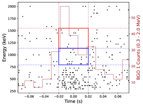
Figure 2: Energetic photons from GRB 231115A are shown, with individual TTEs of the GBM BGO detector 1 indicated by black dots. The blue rectangle highlights energies from approximately 800 keV to 1100 keV, while the red rectangle shows energies ranging from around 1100 keV to 1550 keV. The two events with the highest energies in the blue rectangle, confirmed to be highly likely from the source, are 1049 and 998 keV. Consequently, we conclude that the highest photon energy associated with GRB 231115A is $\sim$13̇,MeV.

2.3 Minimum variability timescale

The minimum variability timescale (MVT) is a measure of the shortest duration of significant fluctuation in the light curve of a GRB. Typically ranging from milliseconds to seconds, these timescales indicate rapid changes in the flux or intensity of a GRB. Given that MGFs can have bulk Lorentz factors ($\Gamma$) that are several orders of magnitude smaller than cosmological GRBs, we expect the MVTs to be much shorter for MGFs. The method of Golkhou et al. (2015), based on Haar-wavelets, yields an MVT of $T_{min}=1.1\,\pm\,0.7\,\rm{ms}$ for GRB 231115A. An independent calculation identifies the MVT as the shortest binning timescale where the GRB signal is distinguishable from background fluctuations (Bhat et al., 2011). This method produces a similar MVT value, $T_{min}=1.1\,\pm\,1.4\,\rm{ms}$. The consistency between these two independently derived values strongly suggests that this is the true MVT for GRB 231115A, enhancing the reliability of our measurement and the robustness of our method. The rise time value (Section 2.1.2) is broadly consistent with the MVTs $T_{rise}=2.7\,\pm\,1.1\,\rm{ms}$. These timescales correspond to an upper limit to the typical emission size, $cT\lesssim 3\times 10^{7}\leavevmode\nobreak\ (T/{\rm ms})\leavevmode\nobreak\ {\rm cm}$.

2.4 Quasi-periodic oscillations

We searched the NaI and BGO data separately for quasi-periodic oscillations (QPOs). First, we generated light curves with a time resolution of $0.122$ ms, allowing us to search up to a frequency of 4096 Hz. We then created Leahy-normalized periodograms from those light curves and found that frequencies above 100 Hz are largely free of burst variability and thus consistent with white noise. We searched the frequency range from 100 to 4096 Hz using standard outlier detection techniques in the linearly and logarithmically binned periodograms and found no credible candidate detection at $p<0.01$, corrected for the number of frequencies searched.

At frequencies below $100\,\mathrm{Hz}$, we implemented the method described in Hübner et al. (2022) and fit a model to the light curve containing an overall burst envelope parameterized as a skewed Gaussian as well as a Damped Random Walk stochastic process. We compared that model to one that also includes a QPO parameterized as a stochastically driven damped harmonic oscillator. We compare models using the Bayes factor and define a strong candidate as one where $\log_{10}(\mathcal{B})>2$. We found a Bayes factor of $\log_{10}(\mathcal{B}_{\mathrm{NaI}})=0.24$ and $\log_{10}(\mathcal{B}_{\mathrm{BGO}})=0.49$ for the NaI and BGO, respectively, and conclude that there is no credible QPO candidate present in the data.

3 Follow-up observations

The detection of GRB 231115A marks the first time that a prompt extragalactic MGF candidate detection and localization (Mereghetti et al., 2024) allowed for rapid follow-up observations by the astronomical community via NASA’s General Coordinates Network (GCN). The rapid follow-up observations detailed in this section provide a compelling case for GRB 231115A as an extragalactic MGF (Mereghetti et al., 2024).

3.1 Gravitational waves

During the occurrence of GRB 231115A, observations were conducted at the LIGO Hanford Observatory (H1) with an approximate average sensitive range of $\sim$150 Mpc for detecting binary neutron star mergers (Ligo Scientific Collaboration et al., 2023). Low-latency pipelines designed for identifying compact binary mergers were operational during this period. Despite this, as stated in Mereghetti et al. (2024), no gravitational-wave candidates were detected within a time window from -5 s to 1 s seconds around GRB 231115A. Notably, the sensitivity of H1 extended to gravitational waves originating from the INTEGRAL sky position.

3.2 X-ray

As reported in Mereghetti et al. (2024), follow-up observations were performed at X-ray wavelengths by Swift/XRT and XMM-Newton. Observations began at $T_{0}+9.0$ ks and $T_{0}+60$ ks for Swift/XRT (Osborne et al., 2023) and XMM-Newton (Rigoselli et al., 2023), respectively. There was no confident detection of a new X-ray source within the burst localization to a depth of $\approx 4\times 10^{-14}$ erg cm^-2 s^-1 in the $2-10$ keV energy range.

However, the arcminute localization uncertainty to GRB 231115A offers a rare opportunity to search for the X-ray counterpart. Here, we briefly discuss the alternatives for such a search, focusing on the capabilities of current satellites and the prospects of future ones.

3.2.1 Persistent source

Magnetars are persistent soft X-ray emitters. The physical picture in this energy range is complex, potentially involving a heterogeneous, hot thermal surface emission modified by a highly magnetized atmosphere (e.g., Viganò, 2013). Despite the small number of known Galactic magnetars, there is a strong indication for a negative correlation between the surface temperature – and consequently soft X-ray luminosity – and the magnetar spin-down age within the population: the younger the magnetar, the brighter the source (e.g., Olausen & Kaspi, 2014b; Viganò et al., 2013; Enoto et al., 2019). Moreover, bursting activity exhibited by younger magnetars tends to be stronger. In fact, the three local magnetars from which the three confirmed MGFs are believed to have originated are among the youngest and brightest of the current population ($L_{\rm X,per}\gtrsim 10^{35}$ erg s^-1). Theoretical simulations of magneto-thermal evolution models (Viganò et al., 2013; Gourgouliatos et al., 2016) and the evolution of crustal stresses, which are responsible for most magnetar activity (Perna & Pons, 2011; Lander & Gourgouliatos, 2019; Lander, 2023), support these observational traits. However, there is a maximum luminosity for magnetar soft thermal emission dictated by neutrino losses in the inner crust: $L_{\rm X,max}\lesssim 10^{36}$ erg s^-1 (e.g., Pons & Rea, 2012).

The galaxy M82 has been observed for a total exposure of approximately 1 Ms with Chandra over the mission’s duration. The luminosity distribution of the Chandra point sources at the INTEGRAL burst position for GRB 231115A ($\pm 4\hbox{${}^{\prime}$}$), as listed in the Chandra source catalog (CSC), is shown in Figure 3 (light gray), along with the distribution of the known magnetar population (dark gray, note that the latter is heavily biased towards the brighter and most active magnetars). The faintest source detected with Chandra has a luminosity of $L_{\rm X}\approx 10^{36}$ erg s^-1, at the limit of the theoretical expectation for the maximum soft X-ray luminosity of a magnetar, though brighter by a factor of two than the brightest known magnetar (SGR 0526$-$66, $L_{\rm X}\approx 5\times 10^{35}$ erg s^-1, Kulkarni et al. 2003; Park et al. 2012). While few of these faint sources might be good magnetar candidates, without enough counts for an adequate spectral and, most importantly, temporal analysis, it is difficult to determine their true nature. Given the high star formation rate in M82, other possible source types include young pulsars, accreting pulsars, high-mass X-ray binaries, and young supernova remnants.

Magnetar persistent soft X-ray emission typically increases during periods of bursting activity, including MGFs (Woods et al., 2001, these epochs are typically referred to as outbursts). However, this emission saturates around $\lesssim 10^{36}$ erg s^-1 (Coti Zelati et al., 2018). Therefore, the prospect of detecting the persistent emission from a magnetar following a MGF, whether during quiescence or an outburst, is slim at distances $\gtrsim 3.5$ Mpc. This situation slightly improves with the next-generation X-ray telescopes. For instance, the sensitivity limit for AXIS, a NASA Probe mission currently under consideration (Reynolds et al., 2023), is about one to two orders of magnitude fainter than Chandra, depending on the spectral shape of the underlying source population, a 250 ks exposure with AXIS reaches a limit of $\approx 10^{-16}$ erg s^-1 cm^-2 for a $5\sigma$ detection, which translates to $10^{35}$ erg s^-1 at 3.5 Mpc (Safi-Harb et al., 2023). The prospect of identifying the magnetar, either through spectral or temporal analyses, is better for nearer galaxies such as Andromeda or M33. However, this limited volume constrains the number density of MGFs. It is clear that identifying the persistent counterpart to a candidate extragalactic MGF (either in quiescence or outburst) will require missions like AXIS and flagship X-ray missions such as Lynx or Athena, the latter planned for a launch in late 2030. Additionally, an intentionally developed IPN could achieve arcsecond localization directly from the event spike.

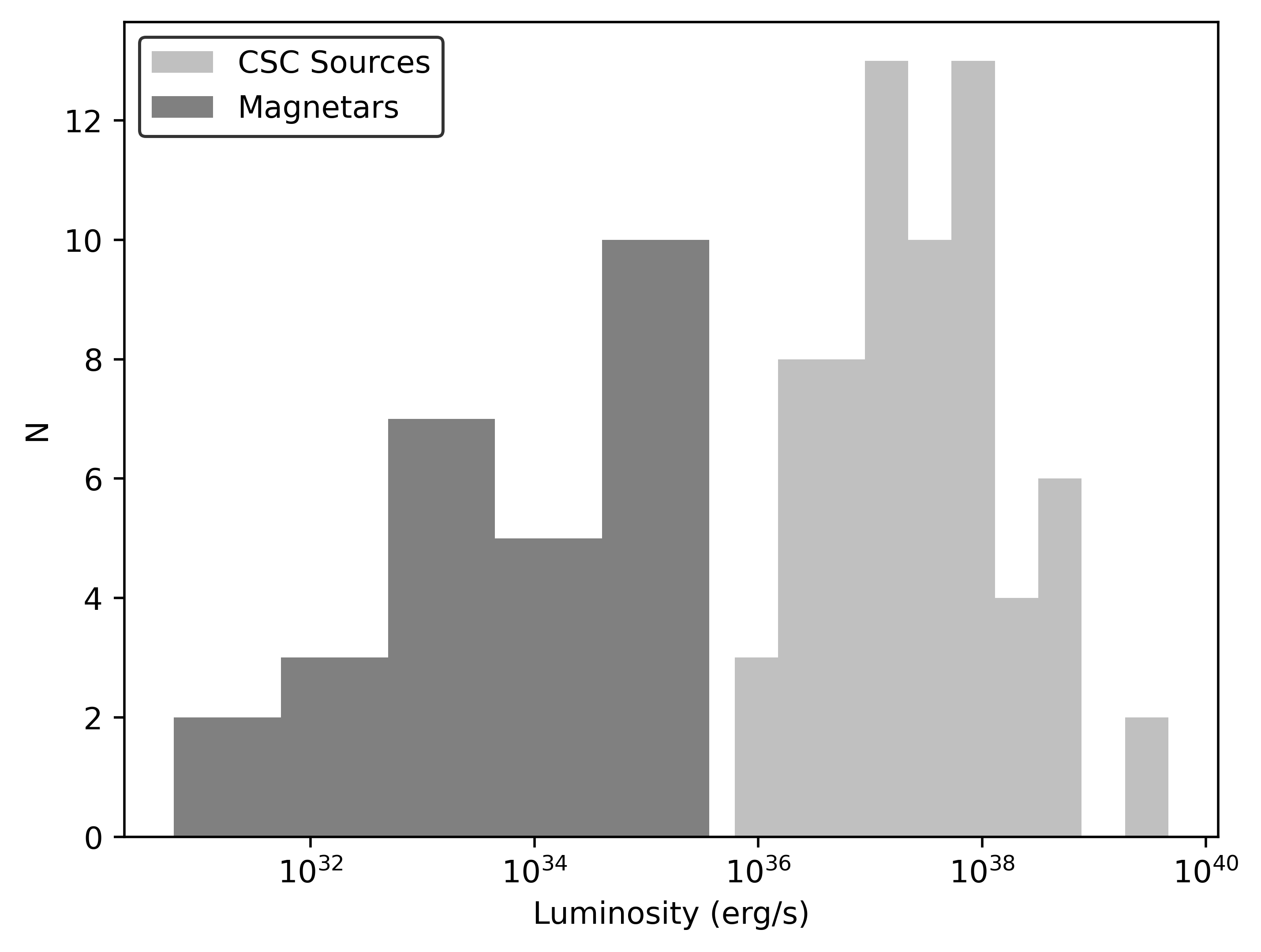
Figure 3: Luminosity distribution of M82 Chandra point sources within the INTEGRAL uncertainty region of GRB 231115A (light gray histogram). These are detected in the full Chandra exposure of the galaxy, totaling $\approx 1$ Ms. The dark gray histogram represents the luminosity distribution of known magnetars.

3.2.2 Bursting magnetar

All three confirmed MGFs were accompanied by short bursts occurring within hours to days following the event (Mazets et al., 1979; Woods et al., 1999; Frederiks et al., 2007a). These short bursts last anywhere from $0.01$ s to $\gtrsim 1$ s and can reach energies on the order of $10^{42}$ erg in the 1-100 keV range. Their energy distribution follows a power-law of the form $dN/dE\propto E^{-\alpha}$ with $\alpha$ in the range 1.5-1.7. The high energy release in the most energetic short bursts provides a rare opportunity for the detection of the counterparts in nearby galaxies with sensitive soft and hard X-ray instruments. This approach has been widely used to search for high-energy counterparts of FRBs with Chandra, XMM-Newton, NICER, and NuSTAR, including the most nearby FRB source in M81 (e.g., Scholz et al., 2017; Laha et al., 2022; Pearlman et al., 2023).

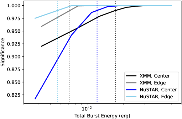
Figure 4: Detectability of short bursts with XMM/Newton (black and gray lines) and NuSTAR (blue and cyan lines), if the putative magnetar is coincident with the center of the galaxy or offset by a few arcminutes, respectively. The vertical dotted lines correspond to burst energy for which a trial-corrected confidence level is at the $99\%$ for each case. See text for more details.

Unlike many FRBs, a precise location (arcsecond localization) and the timing of the presumed bursts are unknown. Hence, we devised a methodology to blind-search for short bursts in imaging data such as XMM-Newton European Photon Imaging Camera (EPIC-PN) and NuSTAR focal plane modules (FPMs) as follows. We produce cleaned images in the 2-10 keV for PN and 3-70 keV ranges for FPMs, centered at the Integral localization $\pm$4^′. We search consecutive one-second frames (with a 0.2 s overlap) within valid good-time-intervals. For this search, we used the SAS tool edetect_chain for PN and the DETECT tool, part of the XIMAGE software for FPMs (Perri et al., 2013). Once candidate sources are flagged by these tools, we compare their excess counts $n$ to the local background rate $\lambda$, determined from the full observation, and calculate the probability that the counts occur randomly, $P_{\rm i}=\lambda^{n_{\rm i}}e^{-\lambda}/n_{\rm i}!$, where index $i$ is for each frame searched. Frames with candidate sources having probability $P_{\rm i}<0.01/N$, where N is the number of frames searched (approximately equal to the livetime in each observation), are considered valid sources at the 99% confidence level (trial corrected). We find no source that passes our criterion for a confident detection in either XMM-Newton or NuSTAR.

We establish the upper-limit on the detectability of short bursts in these observations through simple simulations. We assume the shape of magnetar short bursts’ light curves to be that of a fast-rise exponential-decay (FRED), with rise and decay times set to the average of the distributions taken from the burst forest of SGR 1935+2154 (Younes et al., 2020, see also Gavriil et al. 2004; Scholz & Kaspi 2011). We assume the burst spectra to follow a two-blackbody model with spectral parameters set to the average of the distributions derived from the burst storms of SGR 1935+2154 as observed with Fermi/GBM (Lin et al., 2020). Finally, we vary the 1-100 keV burst energy between $10^{41}$ erg and $10^{43}$ erg logarithmically, in 20 steps. For each simulated burst, the estimated number of counts and their corresponding times and energies are injected into the actual XMM-Newton (or NuSTAR) event file, and our search methodology is repeated. As two extreme cases, we inject the simulated ”source” at the edge of the Integral error circle, away from point sources, and at the bright center of the galaxy.

We find that the short burst fluence detection thresholds, according to our criterion, are $\gtrsim 4\times 10^{-10}$ erg cm^-2 and $\gtrsim 10^{-9}$ erg cm^-2 for the edge and center cases, respectively. This translates to 1-100 keV energies of approximately $6\times 10^{41}$ erg s^-1 and $1.5\times 10^{42}$ erg s^-1, respectively (Figure 4). These figures are similar for XMM/Newton and NuSTAR, and are at the high end of typical short burst energetics, approaching the energies of intermediate flares.

Due to the steep $\log N$-$\log S$ distribution of bursts, our non-detection with PN and FPMs is not surprising. Better prospects can be achieved with HEX-P, yet still at the level of the brightest short magnetar bursts (Alford et al., 2024).

3.2.3 MGF tail detection

The initial spike of the three confirmed MGFs was closely followed by a bright, quasi-thermal hard X-ray tail with an initial luminosity of $L_{\rm X}\approx 10^{42}$ erg s^-1, pulsating at the spin-period of the source (e.g., Mazets et al., 1979; Hurley et al., 1999, 2005; Palmer et al., 2005; Frederiks et al., 2007a). These tails lasted about $400$ seconds before decaying below the sensitivity of large field-of-view instruments. The detection of these tails, especially the pulsations embedded within, serves as smoking-gun evidence of the magnetar central engine for these extreme events.

Currently, the combination of Swift’s Burst Alert Telescope (BAT; Barthelmy et al., 2005) and autonomous repointing to observe with the X-Ray Telescope (XRT; Burrows et al., 2000) is the most promising means by which to capture a MGF tail in time for a possible detection. Unfortunately, for the existing catalog of extragalactic MGF candidates, the source was outside the BAT coded field of view, preventing a possible BAT trigger and the seconds-scale automatic repointing of Swift. Another possible avenue is NICER’s new capability for automatic repointing via a MAXI trigger (OHMAN; Gendreau et al., 2023). However, this is limited by the low rate of short-GRB detection with MAXI, given its limited energy range $2-30$ keV, and NICER visibility, which is complex due to the structure of the International Space Station.

To assess the detectability of MGF tails with Swift and a NICER-like instrument, we simulate the 2004 MGF tail from SGR 1806$-$20 as presented in Hurley et al. (2005) (see also Palmer et al. 2005). The spectrum is modeled as a blackbody with a constant temperature of about 8 keV, folded through the response matrices and effective area curves of Swift/XRT and NICER. The decay follows the evaporating fireball model $L_{\rm x}(t)=L_{0}[1-(t/t_{\rm evap})]^{a/(1-a)}$ with $L_{0}=10^{42}$ erg s^-1 in the 20-100 keV energy range measured at $t\approx 40$ s after the initial spike, $t_{\rm evap}=382$ s, and $a=0.6$ (Hurley et al., 2005). Finally, we modulated the decaying tail at a fiducial spin period of $P=5$ s with a pulse shape following a Fourier series with two harmonics (having approximately equal power; see inset of Figure 5) and an rms pulsed fraction of $45\%$. An example light curve for Swift and NICER at the M82 distance of 3.5 Mpc is shown in the left panel of Figure 5.

The detectability of the tail at extragalactic distances will largely depend on repointing time and the background rate of the instrument. The latter is $\approx 5\times 10^{-3}$ counts s^-1 and $\approx 5\times 10^{-1}$ counts s^-1 for XRT and NICER in the energy range 0.5-10 keV, respectively. For each light curve, we derive the cumulative counts in the tail from a start time ranging from 40 to 300 seconds and compare them to the cumulative background counts in the same time interval. We find that a $3\sigma$ detection (based on a Poisson probability density function for XRT and a Gaussian probability density function for NICER) can be achieved for repointing times of $\lesssim 250$ seconds for both instruments.

However, pulsation detection, shown in the right panel of Figure 5 in the form of the $Z^{2}_{2}$ power, is more prominent in NICER compared to XRT. Varying the distance from 1 Mpc to 20 Mpc reveals that a NICER-like instrument can detect the pulsations in the tail up to a distance of $\sim$6 Mpc, while an XRT-like instrument can do so up to 4 Mpc (Figure 5, right panel). One caveat is that XRT needs to operate in windowed-timing mode to detect pulsations $<5$ seconds due to its limited timing resolution of 2.5 seconds when operating in photon-counting mode.

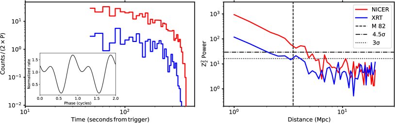
Figure 5: Left panel. Simulated MGF tail light curve with XRT (blue) and NICER (red) assuming the properties as observed in the SGR 1806$-$20 MGF tail, and scaling it to the M82 distance of 3.5 Mpc. The inset shows the modulation that is embedded in the light curve. Right panel. The $Z_{2}^{2}$ power for pulsation detection in XRT and NICER as a function of MGF distance. The dot-dashed and the dotted lines show the 4.5$\sigma$ and 3$\sigma$ detection significance (single-trial), respectively. The vertical dashed line is the M82 distance of 3.5 Mpc. See text for more details.

Identifying the progenitor magnetar of an extragalactic MGF within a few megaparsecs hinges on detecting the X-ray tail, which requires a rapid autonomous response from instruments such as XRT. XRT provides arcsecond localization, which is crucial for studying the magnetar environment—a challenge in the Milky Way due to higher column densities and uncertain distances to Galactic magnetars. The X-ray follow-up of triggers from other satellites is also critical; for example, XRT or NICER could have succeeded in an automated follow-up of an INTEGRAL event. While less probable, a detection by NICER through the OHMAN program could potentially represent the first observation of a pulse period from an extragalactic magnetar. With incremental improvements to currently available technology, the prospects for such detections could significantly improve, e.g., utilizing STROBE-X LEMA- or HEMA-like detectors.

3.3 Optical

Optical follow-up began as early as one hour after the gamma-ray trigger and in Table 2, we present a log of optical observations compiled from GCN Circulars, as reported in Mereghetti et al. (2024) (Chen et al., 2023; Jiang et al., 2023; Kumar et al., 2023; Hayatsu et al., 2023; Turpin et al., 2023; Perley et al., 2023; D’Avanzo et al., 2023; Iskandar et al., 2023; Hu et al., 2023). Additionally, we include our optical follow-up with the 2.1m Fraunhofer telescope (Hopp et al., 2014) at Wendelstein Observatory, Germany.

Observations with the Three Channel Camera (3KK; Lang-Bardl et al., 2016) at Wendelstein Observatory began on 16 November 2023 at 00:39 UT in the $riJH$ filters for two hours. Additional observations were performed on 22 November 2023 at 00:16 UT with the 3KK camera simultaneously in the $riJ$ filters for one hour, and the Wendelstein Wide Field Imager (WWFI; Kosyra et al., 2014) in the $g$ filter for one hour.

Data reduction was performed using a custom pipeline developed at the University Observatory Munich, for both the WWFI and 3KK cameras (Gössl & Riffeser, 2002; Kluge, 2020; Kluge et al., 2020). The pipeline corrects for bias, dark, and flat-field properties and detector artifacts. It uses SCAMP (Bertin, 2006) to compute the astrometric solution with respect to the Gaia EDR3 catalog (Gaia Collaboration et al., 2021), and SWarp (Bertin et al., 2002; Bertin, 2010) to co-add images. Photometric zeropoints were calibrated using nearby stars in the Pan-STARRS-3 Pi (PV3; Magnier et al. 2013) source catalog and Two Micron All Sky Survey (2MASS; Skrutskie et al. 2006) catalog.

Table 2: Log of optical and infrared observations of GRB 231115A.

Start Time (UT)	$T-T_{0}$ (d)	Telescope	Filter	AB Magnitude	Reference
2023-11-15 16:36:59	0.05	GOT	$r$	$>20.1$	Jiang et al. (2023)
2023-11-15 16:46:00	0.05	Lulin	$r$	$>19.2$	Chen et al. (2023)
2023-11-15 16:47:58	0.05	GIT	$r$	$>19.3$	Kumar et al. (2023)
2023-11-15 17:24:23	0.075	MITSuME	$R$	$>19.5$	Hayatsu et al. (2023)
2023-11-15 17:37:53	0.08	GRANDMA	$r$	$>19.3$	Iskandar et al. (2023)
2023-11-15 18:16:33	0.11	MITSuME	$R$	$>20.2$	Hayatsu et al. (2023)
2023-11-15 22:57:23	0.31	OHP	$R$	$>21.1$	Turpin et al. (2023)
2023-11-16 00:39:00	0.375	Wendelstein	$r$	$>22.5$	This work
2023-11-16 00:39:00	0.375	Wendelstein	$i$	$>22.3$	This work
2023-11-16 00:39:00	0.375	Wendelstein	$J$	$>19.7$	This work
2023-11-16 03:27:28	0.49	TNG	$r$	$>22.0$	D’Avanzo et al. (2023)
2023-11-16 03:45:00	0.51	Liverpool	$r$	$>21.6$	Perley et al. (2023)
2023-11-22 00:16:32	6.36	Wendelstein	$r$	–	This work
2023-11-22 00:16:32	6.36	Wendelstein	$i$	–	This work
2023-11-22 00:16:32	6.36	Wendelstein	$J$	–	This work
2023-11-22 02:01:48	6.43	Wendelstein	$g$	$>22.5$	This work

Difference imaging was conducted using the Saccadic Fast Fourier Transform (SFFT) algorithm (Hu et al., 2022). Archival templates from the WWFI, obtained in 2014 in $g$ and $r$ bands, were used as references. For other filters ($i$ and $J$) we performed difference imaging between images acquired on 16 November 2023 and 22 November 2023. Our analysis did not reveal and confidently detect rapidly varying transients between epochs. The $5\sigma$ upper limits for each filter are reported in Table 2.

3.4 Radio

Despite its proximity ($\approx$ 20 degrees) to the CHIME/FRB’s field of view (The CHIME/FRB Collaboration et al., 2021), no radio emission was detected contemporaneously with the high-energy burst. Analysis using established methods constrained potential FRB-like radio emission from GRB 231115A to $<260\,\rm{Jy}$ or $<720\,\rm{Jy\,ms}$, assuming a 10 ms pulse width, at the time of the Fermi/GBM detection. This corresponds to a stringent upper limit on the radio spectral luminosity of $<3.8\times 10^{30}\,\rm{erg\,s^{-1}\,Hz^{-1}}$ at a luminosity distance of 3.5 Mpc to M82 (Curtin & Chime/FRB Collaboration, 2023a).

Prompt limits from CHIME rule out FRB-like events contemporaneous with GRB 231115A (Curtin & Chime/FRB Collaboration, 2023b), both coincident with the Fermi/GBM trigger (although the dispersive delay is unknown) and prior to GRB 231115A. The lack of detection within 80 minutes prior to the Fermi/GBM trigger, despite being directly overhead, results in additional constraints. These constraints limit the radio flux to $<0.5\,\rm{Jy}$ and the fluence to $<1.2\,\rm{Jy\,ms}$, assuming a 10 ms burst width, yielding a radio spectral luminosity limit of $<7.3\times 10^{27}\,\rm{erg\,s^{-1}\,Hz^{-1}}$ (Curtin & Chime/FRB Collaboration, 2023a).

These constraints are highly restrictive, with limits ranging from $<10^{-11}$ to $10^{-9}$ in radio-to-gamma-ray fluence given a flat radio spectral index and band extent of $\sim$ few$\times 10^{8}$ Hz. It remains uncertain whether MGFs can produce prompt FRBs, as the statistics of FRBs resemble those of short bursts rather than MGFs (although shock models favor MGFs, see Popov & Postnov, 2010; Lyubarsky, 2014; Beloborodov, 2017; Metzger et al., 2019). FRB(s) associated with the SGR 1806–20 MGF in 2004 would have been detected by Murriyang (Tendulkar et al., 2016), suggesting that MGFs do not generically result in FRBs. However, from the limited Galactic examples available, MGFs occur during active states of the magnetar, often coinciding with numerous short bursts. Therefore, FRBs could potentially be correlated with MGFs, though not directly caused by them. Patchy observations from 2020-2022 searching for FRBs in M82 yielded limits of $1.2\times 10^{28}$ erg s^-1 Hz^-1 (Paine et al., 2024).

4 Discussion

4.1 Interpreting the spectro-temporal character

Figure 6: The spectra of GRB 231115A over four BB time intervals. The intervals show the onset of the burst (1), peak 1 (2), peak 2 (4), and the extended emission after the peaks (5). Intervals (3), (6), and (7) are omitted for clarity yet still consistent with the trend displayed. The shaded area indicates the $1\sigma$ confidence regions

While the sky association of GRB 231115A with the nearby galaxy M82 is strongly suggestive of a non-cosmological GRB origin for this transient, its spectral evolutionary character provides additional localization-independent arguments for it being a MGF. This is predicated on similarities of its spectral evolution with those of the two MGFs from the Sculptor galaxy, NGC 253, namely GRB 180128A (Trigg et al., 2024) and GRB 200415A (Roberts et al., 2021). The character of this evolution is naturally expected for an intense radiation beam from a rotating magnetar, a model that was highlighted in Roberts et al. (2021). In the absence of an oscillatory tail (discussed in Section 3.2.3, above), the smoking gun signature of a MGF, the initial spike spectral evolution is the main information that can yield insights into the source of these transients.

The rotating, relativistic “lighthouse” picture presumes that the plasma that powers the MGF is blasted off the magnetar surface near the magnetic poles and escapes as a wind to high altitudes and beyond the magnetosphere (e.g., Thompson & Duncan, 1995). This ejection could be triggered by the build-up of magnetic stresses in the crust that eventually force it to crack and release copious amounts of plasma and energy. The highly super-Eddington environment and enormous energy density forces the plasma to flow out at relativistic speeds. This expectation is commensurate with lower limits to the bulk Lorentz factor ($\Gamma$) of the outflow that is obtained from the argument that the emission region is transparent to $\gamma\gamma\to e^{+}e^{-}$ pair creation for all photons up to the maximum energy, $E_{\rm max}$ observed. This transparency is aided by Doppler beaming of the radiation (Krolik & Pier, 1991; Baring, 1993), and $\Gamma>E_{\rm max}/511\,$keV is the most conservative bound possible. Transparency of the emission to two-photon pair creation up to E${}_{max}\sim$ 1.3 MeV (nearly triple the threshold for pair creation) guarantees that the bulk Lorentz factor of the emitting plasma is at least around $\Gamma\sim 3$ relative to the observer, which is less than $\Gamma>6$ that Roberts et al. (2021) obtained for GRB 200415A, which had $E_{\rm max}\sim 3\,$MeV. In contrast, GRB 180128A was somewhat fainter with no photons above 511 keV in energy and above the background level, so $\Gamma>1$ is thereby unconstrained.

The deduced relativistic motion of the plasma automatically implies that the brightness of the flare will vary rapidly and be correlated with its spectral evolution in a fairly well-defined manner dictated by standard special relativistic transformations. As the radiation–plasma beam sweeps across the line of sight to Earth, the luminosity should first intensify and the spectrum should harden to higher energies, and then both should recede (soften) as the beam rotates away from the observer (Roberts et al., 2021). This is the evolutionary sequence seen in both MGF candidates, GRBs 180128A and GRB 200415A.

To determine whether GRB231115A exhibits such an evolutionary sequence, we plotted four of the BB intervals. The results, shown in Figure 6, showcase the spectral evolution from the onset of the burst through the two peaks and into the brief emission that follows. For clarity, the third, sixth, and seventh BB intervals have been omitted from Figure 6, although they align with the overall trend seen in the included intervals. This spectral evolution, characteristic of a MGF, is clearly apparent for GRB 231115A. Such “envelope” behavior is primarily a consequence of the Doppler beaming and boosting from the radiating plasma. This behavior does not naturally arise for classical GRBs born from collapsars or neutron star-neutron star mergers, and so one can conclude that GRB 231115A is likely the initial spike of a MGF.

Figure 7: Comptonized spectrum peak energy ($E_{\mathrm{p}}$) as a function of time using a temporal binning of 8 ms and values from Table 4. All fit errors and error bars are at the 1$\sigma$ confidence level. The zero-time reflects the GBM event start time of each detection.

The $\Delta t\sim 40\,$ms timescale for the overall evolution in Figure 7 can be used to provide a lower bound to the magnetar’s rotation period. This time corresponds to a stellar rotation through an angle $\Delta\theta\sim 2\pi\Delta t/P$ for a rotation period of $P$. For a rotating beam of relativistic plasma, the peak flux of the emission light curve will be approximately confined to the Doppler cone of opening angle $1/\Gamma$, as long as the angular extent of the wind’s collimation is not large. Combining these, one estimates that the putative neutron star’s spin period should be bounded by $P\sim 2\pi\Gamma\,\Delta t\gtrsim 500\,$ms for $\Gamma>2$ for GRB 231115A. In practice, the bulk motion is expected to be somewhat or significantly faster than the pair creation transparency bound suggests. This is mainly due to the plasma dynamics associated with the large amount of energy deposited into the inner magnetosphere over short timescales. It is notable that the detection of delayed GeV-band emission in association with the GRB 200415A giant flare suggested that $\Gamma\sim 100$ was likely (Ajello et al., 2021). If $\Gamma$ lies in the $4-50$ range for GRB 231115A, then the deduced period $P$ would be commensurate with those of Galactic magnetars.

Non-uniformity of the expanding wind naturally yields fluctuations in the Doppler elements, and these are reflected in both the light curve, which has a flux (luminosity) tracer $L_{\mathrm{iso}}$, and the spectroscopy, for which we use $E_{\mathrm{p}}$ as a hardness marker. In Figure 8, we illustrate that these two quantities are fairly tightly correlated for GRB 231115A and prior MGFs approximately via the $L_{\mathrm{iso}}\propto E_{\mathrm{p}}^{\beta}$ form listed in Eq. (3). Roberts et al. (2021) emphasized that theoretically, the index $\beta$ should be tightly coupled to the dual relativistic elements of Doppler boosting (influencing $E_{\mathrm{p}}\propto\Gamma$) and Doppler beaming (enhancing $L_{\mathrm{iso}}$). As was detailed in Trigg et al. (2024), the actual value of the index $\beta$ should depend on the temporal sampling of the light curve, ranging from $\beta\sim 2$ for approximately uniform time bins (see Figure 8a), to $\beta\sim 4$ for BB time intervals (see Figure 8b). The physical origin of these two extremes is linked to the size of the lookback surface within the relativistic wind that is sampled during the time intervals. The BB choice yields partial samplings of smaller surface sizes that capture more of the Doppler flux beaming character $L_{\mathrm{iso}}\propto\Gamma^{4}$. Performing spectroscopy on uniform time bin selections tends to smear out the surface solid angle sampling fluctuations, emphasizing the photon energy boosting and time dilation characteristics, generating $L_{\mathrm{iso}}\propto\Gamma^{2}$ (Trigg et al., 2024). For GRB 231115A, the reality is between these two extremes, as it is for the other MGFs addressed in Figure 8 and discussed in Trigg et al. (2024). Yet the fact that a steeper $L_{\mathrm{iso}}-E_{\mathrm{p}}$ correlation is evinced for the BB choice does indicate that the physical angular extent of the wind is modest or small, commensurate with expectations of a wind anchored to open field lines emerging from the magnetar’s polar surface.

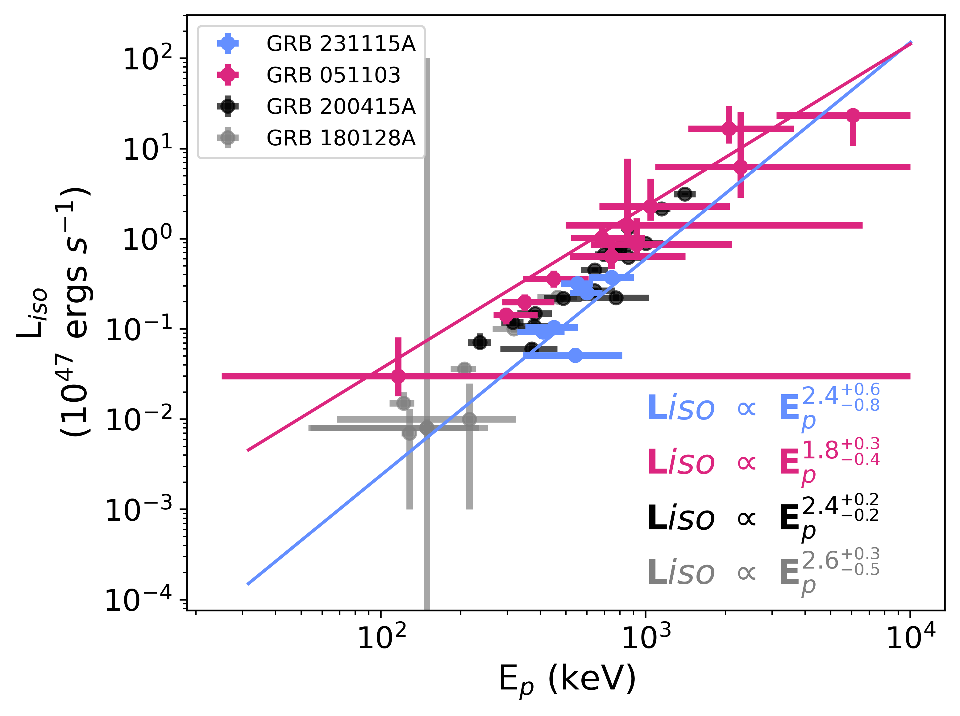
(a)

(b)

Figure 8: Left (a): Correlation between $L_{\mathrm{iso}}$ and $E_{\mathrm{p}}$ for the four MGF candidates, GRB 231115A (light blue) and GRB 051103 (pink) plotted alongside GRB 200415A (black) and GRB 80128A (gray), revealing an approximate $L_{\mathrm{iso}}$ $\propto$ $E_{\mathrm{p}}^{2}$ relationship that is a strong signature of relativistic winds. The temporal binning for panel (a) is uniformly fixed intervals and uses the values in Table 4. Right (b): $L_{\mathrm{iso}}$ and $E_{\mathrm{p}}$ for all four transients over the BB intervals in Tables 1 and 3, omitting the unconstrained $E_{\rm{p}}$ intervals of GRB 051103. These data were fit using the fitting method described in Appendix 3, which is able to fit data with asymmetric uncertainties. All fit uncertainties and uncertainty bars are at the 1$\sigma$ confidence level.

5 Conclusion

The detection and analysis of GRB 231115A provide compelling evidence of an extragalactic MGF originating from the starburst galaxy M82. This burst gives a fully self-consistent picture based on the model discussed in Section 4.1. The observed spectral evolution closely mirrors the characteristics of known MGFs from other galaxies, such as NGC 253, supporting the classification of GRB 231115A as a MGF. The comprehensive gamma-ray analysis conducted with Fermi/GBM data revealed significant insights into the burst’s properties, including its high peak energy and complex temporal structure. The association of GRB 231115A with M82 was further strengthened by the high Bayes factor, suggesting a very low probability of a chance alignment with a cosmological neutron star merger.

The detection of high-energy photons double the threshold for $\gamma\gamma$ pair creation confirms a lower limit on the bulk Lorentz factor ($\Gamma\gtrsim 2$) of the outflowing plasma, consistent with expectations for relativistic winds from magnetars and is comparable to observations from previous MGFs like GRB 200415A and GBR 180128A. Moreover, the MVT indicates rapid flux changes typical of MGFs. This short timescale aligns with the smaller Lorentz factors expected for MGFs compared to cosmological GRBs, further supporting our classification.

This discovery not only adds to the growing list of extragalactic MGF candidates but also emphasizes the importance of prompt and coordinated multi-wavelength follow-up observations in understanding these rare and energetic events. The ability to detect and accurately localize such MGFs in distant galaxies opens up new avenues for studying magnetars and their environments outside our Galaxy. The detectability of MGF tails at extragalactic distances is crucial, as they provide unambiguous evidence for magnetar central engines. Simulations show that the detectability of the tail depends significantly on repointing time and instrument background rates. The limitations in detecting and characterizing MGFs with current instruments underscore the importance of new technologies and coordinated multi-wavelength observations. Proposed missions and next-generation X-ray satellites are critical for advancing our understanding of these phenomena.

The detection of GRB 231115A and unambiguous localization to M82 underscores the contribution of MGFs to the population of short GRBs. Future advancements in observational technology and methodologies, such as rapid automated repointing and increased X-ray sensitivity, will likely enhance our capacity to identify and study these phenomena, thereby furthering our understanding of the mechanisms driving short GRBs and the role of magnetars in the cosmos.

Appendix A $L_{\mathrm{iso}}$ - $E_{\mathrm{p}}$ relation fitting method

In previous analyses of the luminosity-hardness correlation relationship between $L_{\mathrm{iso}}$ and $E_{\mathrm{p}}$, such as those in Roberts et al. (2021) and Trigg et al. (2024), data fitting used the assumptions of symmetric errors for the dependent ($L_{\mathrm{iso}}$) and independent variables ($E_{\mathrm{p}}$), sometimes even ignoring the errors in the $E_{\mathrm{p}}$ entirely, as is common in least-squares regression. To better constrain the fit values for the $L_{\mathrm{iso}}$–$E_{\mathrm{p}}$ relation of GRB 231115A and GRB 051103, as well as reevaluate GRB 200415A, and GRB 180128A, we use statistical methods that account for asymmetric errors in both variables. This method allows for the unbiased determination of probability distributions for the model parameters of interest.

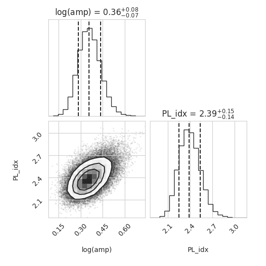
(a)

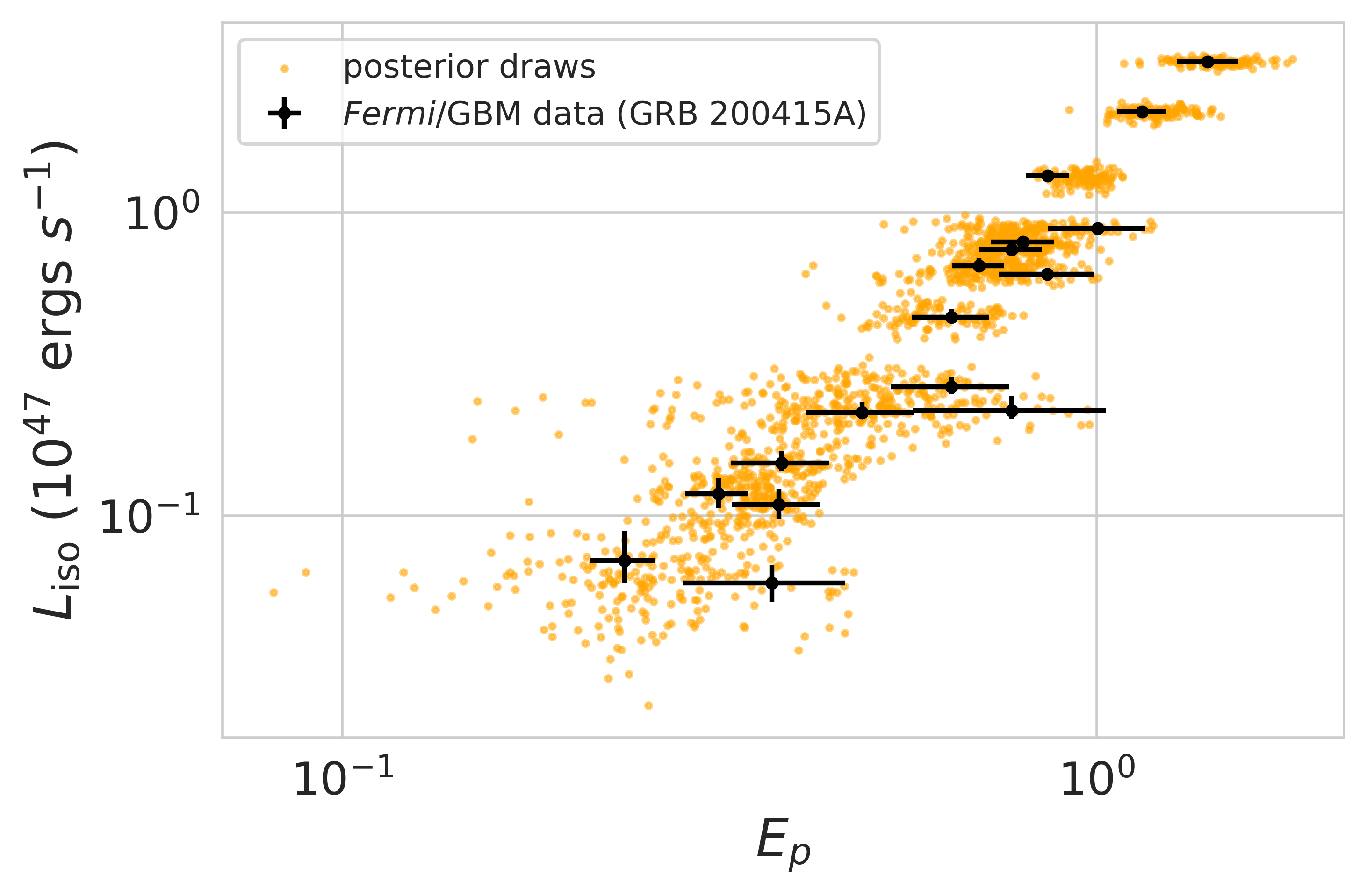
(b)

Figure 9: Left (a): Corner plot of posterior distributions for the two power-law parameters describing the relationship between the peak energy and isotropic luminosity. Right (b): Data-resolved spectroscopy of the Fermi/GBM data for GRB 200415A (black) and the posterior predictive distribution (orange). To compute the posterior predictive distribution we simulated the data generation process by first picking a set of parameters ($(\{\hat{E}_{p,i,k}\}_{i=1}^{N},\alpha_{k},\beta_{k})$) from the posterior, then generating random simulated values for $L_{\mathrm{iso,sim}}^{*}$ and $E_{p,\mathrm{sim}^{*}}$ using the TPN distribution. This figure shows 100 such simulated data sets and enables a convenient comparison of the performance of the model with the data.

Errors on both $E_{p}$ and $L_{\mathrm{iso}}$ are heteroscedastic (different for each data point) and asymmetric. To model the asymmetric errors in each dimension, we use a Two-Piece Normal (TPN) distribution as proposed by Fernández & Steel (1998). This distribution corresponds to two half-normal distributions with standard deviations $\sigma_{1}$ (left-hand side) and $\sigma_{2}$ (right-hand side), joined at a common mode $\mu$ and re-normalized such that the distribution is continuous. This distribution is usually parametrized by a common standard deviation $\sigma$ and a skewness $\lambda$, with the probability density then being

$$p(x,\mu,\sigma,\lambda)=\begin{cases}\frac{2\lambda}{(1+\lambda^{2})\sigma}\phi\left(\frac{\lambda(x-\mu)}{\sigma}\right)\,,\;\mathrm{if}\,x<\mu;\\ \frac{2\lambda}{(1+\lambda^{2})\sigma}\phi\left(\frac{x-\mu}{\lambda\sigma}\right)\,,\;\mathrm{if}\,x\geq\mu\,,\end{cases}$$ (1)

where

$$\sigma = \sigma_{1}$$ (2)

$$\lambda = \sqrt{\sigma_{2}/\sigma_{1}}\;.$$

The latter two equations enable the straightforward conversion of asymmetric errors as reported in the astronomical literature into a single standard deviation and skewness for use with the TPN.

To account for the presence of errors in both variables, we build an errors-in-variables model. Our data consists of pairs of observed values $\{E_{p}^{*},L_{\mathrm{iso}}^{*}\}$. We assume that the observed $E_{p}^{*}$ are random variables drawn from a TPN distribution with a mean given by a set of unknown true $\hat{E}_{p}$ values. To identify the luminosity-hardness correlation, we assume a standard power-law relationship between the variables of the form

$$\hat{L}_{\mathrm{iso}}=\alpha\hat{E}_{p}^{\beta}\quad.$$ (3)

Note that this relationship holds between the (unknown) true peak energy and isotropic luminosity, not the observed quantities. Whereas a standard likelihood assumes that the $\hat{E}_{p}$ are known, the errors-in-variables model infers them along with the parameters of the relationship, such that the total number of parameters to be inferred becomes $(\{\hat{E}_{p,i}\}_{i=1}^{N},\alpha,\beta)$, for $N$ data points, a power law amplitude $\alpha$ and a power law index $\beta$. We infer the parameters in a Bayesian framework:

$$p(\alpha,\beta,\{\hat{E}_{p,i}\}_{i=1}^{N}|E_{p}^{*},L_{\mathrm{iso}}^{*})\propto p(L_{\mathrm{iso}}^{*}|\hat{E}_{p},\alpha,\beta)p(E_{p}^{*}|\hat{E}_{p})p(\alpha,\beta,\hat{E}_{p})\;.$$ (4)

Intuitively, this model parametrizes the data generation process: a power-law relationship exists between the unknown true peak energies and the unknown true isotropic luminosities. We first parametrize the relationship between the true peak energies and observed peak energies using the TPN distribution, and draw from it as well as the priors for the other parameters $\alpha$ and $\beta$. We can assume conditional independence such that the priors for all parameters can be written independently:

$$p(\alpha,\beta,\hat{E}_{p})=p(\alpha)p(\beta)p(\hat{E}_{p})\;.$$

The observed isotropic luminosities are then governed by a power-law relationship between the sampled true $\hat{E}_{p}$ and true, unknown $\hat{L}_{\mathrm{iso}}$, given parameters $\alpha$ and $\beta$, and compared to the observed $L^{*}_{\mathrm{iso}}$ through a likelihood $p(L_{\mathrm{iso}}^{*}|\hat{E}_{p},\alpha,\beta)\sim\mathrm{TPN}(\hat{L}_{\mathrm{iso}},\sigma_{L},\lambda_{L})$, where $\sigma_{L}$ and $\lambda_{L}$ are the standard deviation and skewness for $L^{*}_{\mathrm{iso}}$ as defined using Equation 2 above.

This model can be sampled with Markov Chain Monte Carlo in order to infer the true $\hat{E}_{p}$ and the power law parameters $\alpha$ and $\beta$. To do so, one first samples $\hat{E}_{p}$ from a prior distribution, and then computes a likelihood $p(E_{p}^{*}|\hat{E}_{p})$ for the observed peak energy given the true peak energy using the TPN distribution. In a second step, the $\hat{E}_{p}$ values are used to compute the proposed power law relationship, together with $\alpha$ and $\beta$, also sampled from a prior. This relationship is then compared to the observed $L_{\mathrm{iso}}^{*}$, again using a TPN distribution to obtain the posterior probability for the parameters. This model enables us to effectively take into account the asymmetric uncertainties on both peak energy and isotropic luminosity.

We set uninformative, flat priors on all parameters, where the prior for peak energies are defined as $\hat{E}_{p}\sim\mathcal{U}(0\,\mathrm{keV},15\,\mathrm{keV})$, the prior on the power law index is $\beta\sim\mathcal{U}(1,4)$ and the prior on the natural logarithm of the amplitude is $\log(\alpha)\sim\mathcal{U}(-2,4)$, where $\mathcal{U}(a,b)$ denotes a uniform distribution between lower boundary $a$ and upper boundary $b$.

We implement the model in the probabilistic programming language numpyro (Phan et al. 2019; Bingham et al. 2019), and use Hamiltonian Monte Carlo with the No U-Turn Sampler (NUTS) (Homan & Gelman 2014) to sample the posteriors for all parameters. We run six HMC chains with 4,000 warmup steps and 10,000 sampling steps. We assess convergence using autocorrelation time and the Gelman-Rubin statistic and find that all chains are well-converged ($T_{\mathrm{GR}}\leq 1.001$ for all parameters).

Figure 9 shows the results of the modeling for GRB 200415A. We chose this burst as it has good count statistics and the luminosity-hardness correlation has been derived by several previous studies (Roberts et al. 2021; Trigg et al. 2024). The posterior for the parameters is well-constrained and single-peaked, with a power-law index of $\beta=2.39^{+0.15}_{-0.14}$, marginalized over the uncertainties in $E_{p}$. Similarly, the posterior predictive distribution mirrors the observed data well, suggesting that the model overall can represent the data effectively.

Appendix B Time-resolved spectral analysis

Table 3: Time-resolved spectral analysis using Bayesian Blocks

Time	$E_{\mathrm{p}}$	$\alpha$	Energy Flux ($\cal{F}$)	$L_{\mathrm{iso}}$	$E_{\mathrm{iso}}$
(ms)	(keV)		($\times 10^{-6}$ ergs s-1 cm-2)	($\times 10^{45}$ erg$\cdot$ s-1)	($\times 10^{44}$ erg)
GRB 200415A
-4.3:-3.9	570 $\begin{subarray}{c}+90\\ -800\end{subarray}$	-0.2 $\begin{subarray}{c}+0.3\\ -0.3\end{subarray}$	134 $\begin{subarray}{c}+6\\ -6\end{subarray}$	196 $\begin{subarray}{c}+5\\ -4\end{subarray}$	0.81 $\begin{subarray}{c}+0.02\\ -0.02\end{subarray}$
-3.9:-3.4	800 $\begin{subarray}{c}+200\\ -200\end{subarray}$	-0.5 $\begin{subarray}{c}+0.3\\ -0.2\end{subarray}$	230 $\begin{subarray}{c}+20\\ -20\end{subarray}$	341 $\begin{subarray}{c}+20\\ -12\end{subarray}$	1.79 $\begin{subarray}{c}+0.01\\ -0.01\end{subarray}$
-3.4:-2.9	860 $\begin{subarray}{c}+120\\ -100\end{subarray}$	-0.33 $\begin{subarray}{c}+0.15\\ -0.15\end{subarray}$	410 $\begin{subarray}{c}+20\\ -20\end{subarray}$	600 $\begin{subarray}{c}+20\\ -10\end{subarray}$	3.1 $\begin{subarray}{c}+0.1\\ -0.1\end{subarray}$
-2.9:-2.5	890 $\begin{subarray}{c}+140\\ -120\end{subarray}$	-0.2 $\begin{subarray}{c}+0.2\\ -0.2\end{subarray}$	610 $\begin{subarray}{c}+30\\ -30\end{subarray}$	890 $\begin{subarray}{c}+30\\ -20\end{subarray}$	3.65 $\begin{subarray}{c}+0.13\\ -0.07\end{subarray}$
-2.5:-0.5	1350 $\begin{subarray}{c}+150\\ -130\end{subarray}$	-0.3 $\begin{subarray}{c}+0.1\\ -0.1\end{subarray}$	710 $\begin{subarray}{c}+20\\ -30\end{subarray}$	1040 $\begin{subarray}{c}+20\\ -20\end{subarray}$	21.2 $\begin{subarray}{c}+0.5\\ -0.4\end{subarray}$
-0.5:3.0	1800 $\begin{subarray}{c}+200\\ -200\end{subarray}$	-0.08 $\begin{subarray}{c}+0.08\\ -0.08\end{subarray}$	610 $\begin{subarray}{c}+20\\ -20\end{subarray}$	900 $\begin{subarray}{c}+30\\ -10\end{subarray}$	32.1 $\begin{subarray}{c}+0.7\\ -0.5\end{subarray}$
3.0:5.0	900 $\begin{subarray}{c}+200\\ -200\end{subarray}$	0.1 $\begin{subarray}{c}+0.3\\ -0.3\end{subarray}$	112 $\begin{subarray}{c}+7\\ -7\end{subarray}$	160 $\begin{subarray}{c}+10\\ -10\end{subarray}$	3.44 $\begin{subarray}{c}+0.13\\ -0.11\end{subarray}$
5.0:6.5	800 $\begin{subarray}{c}+300\\ -300\end{subarray}$	1.0 $\begin{subarray}{c}+0.7\\ -1.1\end{subarray}$	17 $\begin{subarray}{c}+5\\ -6\end{subarray}$	24 $\begin{subarray}{c}+5\\ -4\end{subarray}$	0.4 $\begin{subarray}{c}+0.1\\ -0.1\end{subarray}$
6.5:22.5	1040 $\begin{subarray}{c}+50\\ -50\end{subarray}$	0.8 $\begin{subarray}{c}+0.1\\ -0.1\end{subarray}$	119 $\begin{subarray}{c}+5\\ -5\end{subarray}$	174 $\begin{subarray}{c}+5\\ -3\end{subarray}$	28.5 $\begin{subarray}{c}+0.8\\ -0.5\end{subarray}$
22.5:65.8	800 $\begin{subarray}{c}+40\\ -40\end{subarray}$	0.5 $\begin{subarray}{c}+0.1\\ -0.1\end{subarray}$	50 $\begin{subarray}{c}+2\\ -2\end{subarray}$	73 $\begin{subarray}{c}+2\\ -1\end{subarray}$	32.3 $\begin{subarray}{c}+0.6\\ -0.4\end{subarray}$
65.8:93.3	570 $\begin{subarray}{c}+50\\ -50\end{subarray}$	0.3 $\begin{subarray}{c}+0.3\\ -0.3\end{subarray}$	18.4 $\begin{subarray}{c}+1.1\\ -1.0\end{subarray}$	27 $\begin{subarray}{c}+1\\ -1\end{subarray}$	7.7 $\begin{subarray}{c}+0.4\\ -0.2\end{subarray}$
93.3:121.2	420 $\begin{subarray}{c}+40\\ -30\end{subarray}$	0.8 $\begin{subarray}{c}+0.6\\ -0.5\end{subarray}$	9.2 $\begin{subarray}{c}+0.8\\ -0.8\end{subarray}$	14 $\begin{subarray}{c}+1\\ -1\end{subarray}$	4.0 $\begin{subarray}{c}+0.3\\ -0.2\end{subarray}$
121.2:150.2	250 $\begin{subarray}{c}+30\\ -20\end{subarray}$	1.0 $\begin{subarray}{c}+0.7\\ -0.5\end{subarray}$	3.2 $\begin{subarray}{c}+0.8\\ -0.8\end{subarray}$	5 $\begin{subarray}{c}+1\\ -1\end{subarray}$	1.6 $\begin{subarray}{c}+0.3\\ -0.1\end{subarray}$
GRB 180128A
-12.0:-10.0	180 $\begin{subarray}{c}+20\\ -20\end{subarray}$	4.3 $\begin{subarray}{c}+1.1\\ -0.9\end{subarray}$	7 $\begin{subarray}{c}+2\\ -2\end{subarray}$	10 $\begin{subarray}{c}+3\\ -2\end{subarray}$	0.25 $\begin{subarray}{c}+0.05\\ -0.03\end{subarray}$
-10.0:-7.0	510 $\begin{subarray}{c}+120\\ -100\end{subarray}$	0.05 $\begin{subarray}{c}+0.58\\ -0.47\end{subarray}$	37 $\begin{subarray}{c}+2\\ -2\end{subarray}$	54 $\begin{subarray}{c}+3\\ -2\end{subarray}$	1.7 $\begin{subarray}{c}+0.1\\ -0.1\end{subarray}$
-7.0:-3.0	400 $\begin{subarray}{c}+40\\ -60\end{subarray}$	5 $\begin{subarray}{c}+2\\ -3\end{subarray}$	7 $\begin{subarray}{c}+2\\ -3\end{subarray}$	10 $\begin{subarray}{c}+2\\ -1\end{subarray}$	0.5 $\begin{subarray}{c}+0.1\\ -0.1\end{subarray}$
-3.0:-1.0	400 $\begin{subarray}{c}+110\\ -100\end{subarray}$	0.4 $\begin{subarray}{c}+1.0\\ -0.7\end{subarray}$	23 $\begin{subarray}{c}+4\\ -3\end{subarray}$	33 $\begin{subarray}{c}+4\\ -2\end{subarray}$	0.73 $\begin{subarray}{c}+0.08\\ -0.04\end{subarray}$
-1.0:18.0	180 $\begin{subarray}{c}+10\\ -11\end{subarray}$	4.0 $\begin{subarray}{c}+0.7\\ -0.6\end{subarray}$	2.4 $\begin{subarray}{c}+0.4\\ -0.3\end{subarray}$	3.6 $\begin{subarray}{c}+0.4\\ -0.2\end{subarray}$	0.8 $\begin{subarray}{c}+0.1\\ -0.1\end{subarray}$
18.0:143.0	140 $\begin{subarray}{c}+20\\ -20\end{subarray}$	0.8 $\begin{subarray}{c}+0.4\\ -0.3\end{subarray}$	0.5 $\begin{subarray}{c}+0.1\\ -0.1\end{subarray}$	0.7 $\begin{subarray}{c}+0.2\\ -0.1\end{subarray}$	1.0 $\begin{subarray}{c}+0.2\\ -0.1\end{subarray}$

Table 4: Fixed time intervals

Time	$E_{\mathrm{p}}$	$\alpha$	Energy Flux ($\cal{F}$)	$L_{\mathrm{iso}}$	$E_{\mathrm{iso}}$
(ms)	(keV)		($\times 10^{-6}$ ergs s-1 cm-2)	($\times 10^{45}$ erg$\cdot$ s-1)	($\times 10^{44}$ erg)
GRB 231115A
-16.0:-8.0	550 $\begin{subarray}{c}+80\\ -70\end{subarray}$	0.5 $\begin{subarray}{c}+0.5\\ -0.5\end{subarray}$	22 $\begin{subarray}{c}+2\\ -2\end{subarray}$	32 $\begin{subarray}{c}+3\\ -2\end{subarray}$	2.7 $\begin{subarray}{c}+0.2\\ -0.12\end{subarray}$
-8.0:0.0	740 $\begin{subarray}{c}+160\\ -130\end{subarray}$	0.1 $\begin{subarray}{c}+0.4\\ -0.4\end{subarray}$	25 $\begin{subarray}{c}+2\\ -2\end{subarray}$	37 $\begin{subarray}{c}+2\\ -1\end{subarray}$	3.14 $\begin{subarray}{c}+0.14\\ -0.11\end{subarray}$
0.0:8.0	600 $\begin{subarray}{c}+90\\ -80\end{subarray}$	0.9 $\begin{subarray}{c}+0.5\\ -0.6\end{subarray}$	17 $\begin{subarray}{c}+2\\ -2.\end{subarray}$	25.2 $\begin{subarray}{c}+2.3\\ -1.1\end{subarray}$	2.19 $\begin{subarray}{c}+0.20\\ -0.012\end{subarray}$
8.0:16.0	410 $\begin{subarray}{c}+90\\ -80\end{subarray}$	0.8 $\begin{subarray}{c}+1.5\\ -1.1\end{subarray}$	6 $\begin{subarray}{c}+1\\ -2\end{subarray}$	9.3 $\begin{subarray}{c}+1.4\\ -0.7\end{subarray}$	0.85 $\begin{subarray}{c}+0.11\\ -0.07\end{subarray}$
16.0:24.0	500 $\begin{subarray}{c}+100\\ -100\end{subarray}$	0.7 $\begin{subarray}{c}+1.2\\ -1.0\end{subarray}$	7 $\begin{subarray}{c}+2\\ -2\end{subarray}$	10 $\begin{subarray}{c}+2\\ -1\end{subarray}$	0.94 $\begin{subarray}{c}+0.12\\ -0.08\end{subarray}$
24.0:44.0	500 $\begin{subarray}{c}+300\\ -200\end{subarray}$	-0.2 $\begin{subarray}{c}+0.9\\ -0.7\end{subarray}$	3.5 $\begin{subarray}{c}+1.0\\ -0.8\end{subarray}$	5.1 $\begin{subarray}{c}+1.1\\ -0.7\end{subarray}$	1.21 $\begin{subarray}{c}+0.20\\ -0.14\end{subarray}$
GRB 200415A
-8.0:0.0	1190 $\begin{subarray}{c}+120\\ -110\end{subarray}$	-0.3 $\begin{subarray}{c}+0.1\\ -0.1\end{subarray}$	276 $\begin{subarray}{c}+8\\ -8\end{subarray}$	404 $\begin{subarray}{c}+9\\ -6\end{subarray}$	33.0 $\begin{subarray}{c}+0.8\\ -0.5\end{subarray}$
0.0:8.0	1400 $\begin{subarray}{c}+140\\ -130\end{subarray}$	0.1 $\begin{subarray}{c}+0.1\\ -0.1\end{subarray}$	214 $\begin{subarray}{c}+7\\ -7\end{subarray}$	314 $\begin{subarray}{c}+8\\ -4\end{subarray}$	25.6 $\begin{subarray}{c}+0.7\\ -0.4\end{subarray}$
8.0:16.0	1150 $\begin{subarray}{c}+90\\ -90\end{subarray}$	0.6 $\begin{subarray}{c}+0.1\\ -0.1\end{subarray}$	146 $\begin{subarray}{c}+7\\ -8\end{subarray}$	215 $\begin{subarray}{c}+7\\ -5\end{subarray}$	17.8 $\begin{subarray}{c}+0.6\\ -0.4\end{subarray}$
16.0:24.0	860 $\begin{subarray}{c}+60\\ -60\end{subarray}$	1.1 $\begin{subarray}{c}+0.2\\ -0.2\end{subarray}$	90 $\begin{subarray}{c}+5\\ -6\end{subarray}$	132 $\begin{subarray}{c}+5\\ -4\end{subarray}$	11.0 $\begin{subarray}{c}+0.5\\ -0.3\end{subarray}$
24.0:32.0	1000 $\begin{subarray}{c}+200\\ -140\end{subarray}$	0.03 $\begin{subarray}{c}+0.20\\ -0.20\end{subarray}$	61 $\begin{subarray}{c}+3\\ -3\end{subarray}$	89 $\begin{subarray}{c}+3\\ -3\end{subarray}$	7.3 $\begin{subarray}{c}+0.2\\ -0.2\end{subarray}$
32.0:40.0	770 $\begin{subarray}{c}+80\\ -70\end{subarray}$	0.7 $\begin{subarray}{c}+0.2\\ -0.2\end{subarray}$	52 $\begin{subarray}{c}+4\\ -4\end{subarray}$	76 $\begin{subarray}{c}+4\\ -3\end{subarray}$	6.3 $\begin{subarray}{c}+0.4\\ -0.2\end{subarray}$
40.0:48.0	800 $\begin{subarray}{c}+80\\ -80\end{subarray}$	0.7 $\begin{subarray}{c}+0.2\\ -0.2\end{subarray}$	54 $\begin{subarray}{c}+4\\ -4\end{subarray}$	80 $\begin{subarray}{c}+5\\ -3\end{subarray}$	6.7 $\begin{subarray}{c}+0.3\\ -0.3\end{subarray}$
48.0:56.0	700 $\begin{subarray}{c}+60\\ -50\end{subarray}$	1.2 $\begin{subarray}{c}+0.2\\ -0.3\end{subarray}$	46 $\begin{subarray}{c}+3\\ -4\end{subarray}$	67 $\begin{subarray}{c}+4\\ -2\end{subarray}$	6.0 $\begin{subarray}{c}+0.3\\ -0.2\end{subarray}$
56.0:64.0	860 $\begin{subarray}{c}+130\\ -120\end{subarray}$	0.2 $\begin{subarray}{c}+0.2\\ -0.3\end{subarray}$	43 $\begin{subarray}{c}+3\\ -3\end{subarray}$	63 $\begin{subarray}{c}+4\\ -2\end{subarray}$	5.2 $\begin{subarray}{c}+0.3\\ -0.2\end{subarray}$
64.0:72.0	640 $\begin{subarray}{c}+80\\ -70\end{subarray}$	0.6 $\begin{subarray}{c}+0.3\\ -0.4\end{subarray}$	31 $\begin{subarray}{c}+3\\ -3\end{subarray}$	45 $\begin{subarray}{c}+3\\ -2\end{subarray}$	3.8 $\begin{subarray}{c}+0.2\\ -0.1\end{subarray}$
72.0:80.0	640 $\begin{subarray}{c}+120\\ -110\end{subarray}$	0.2 $\begin{subarray}{c}+0.4\\ -0.5\end{subarray}$	18 $\begin{subarray}{c}+2\\ -2\end{subarray}$	26.6 $\begin{subarray}{c}+2.4\\ -1.4\end{subarray}$	2.3 $\begin{subarray}{c}+0.2\\ -0.1\end{subarray}$
80.0:88.0	490 $\begin{subarray}{c}+80\\ -80\end{subarray}$	0.3 $\begin{subarray}{c}+0.6\\ -0.6\end{subarray}$	15 $\begin{subarray}{c}+2\\ -2\end{subarray}$	21.9 $\begin{subarray}{c}+1.6\\ -1.0\end{subarray}$	2.0 $\begin{subarray}{c}+0.1\\ -0.1\end{subarray}$
88.0:96.0	380 $\begin{subarray}{c}+60\\ -60\end{subarray}$	0.6 $\begin{subarray}{c}+1.3\\ -0.8\end{subarray}$	10.2 $\begin{subarray}{c}+1.3\\ -1.5\end{subarray}$	14.9 $\begin{subarray}{c}+1.5\\ -0.9\end{subarray}$	1.28 $\begin{subarray}{c}+0.11\\ -0.06\end{subarray}$
96.0:104.0	800 $\begin{subarray}{c}+300\\ -200\end{subarray}$	-0.12 $\begin{subarray}{c}+0.43\\ -0.47\end{subarray}$	15 $\begin{subarray}{c}+2\\ -2\end{subarray}$	22 $\begin{subarray}{c}+3\\ -2\end{subarray}$	2.0 $\begin{subarray}{c}+0.2\\ -0.2\end{subarray}$
104.0:112.0	380 $\begin{subarray}{c}+50\\ -50\end{subarray}$	1.4 $\begin{subarray}{c}+1.5\\ -1.2\end{subarray}$	7.4 $\begin{subarray}{c}+1.5\\ -9.1\end{subarray}$	10.9 $\begin{subarray}{c}+1.8\\ -1.1\end{subarray}$	1.01 $\begin{subarray}{c}+0.11\\ -0.10\end{subarray}$
112.0:120.0	320 $\begin{subarray}{c}+30\\ -30\end{subarray}$	1.9 $\begin{subarray}{c}+3.2\\ -1.3\end{subarray}$	8 $\begin{subarray}{c}+2\\ -2\end{subarray}$	11.8 $\begin{subarray}{c}+2.0\\ -1.1\end{subarray}$	1.08 $\begin{subarray}{c}+0.14\\ -0.10\end{subarray}$
120.0:128.0	240 $\begin{subarray}{c}+20\\ -20\end{subarray}$	2.2 $\begin{subarray}{c}+1.2\\ -0.8\end{subarray}$	4.9 $\begin{subarray}{c}+2.0\\ -1.1\end{subarray}$	7.1 $\begin{subarray}{c}+1.5\\ -1.2\end{subarray}$	0.69 $\begin{subarray}{c}+0.14\\ -0.08\end{subarray}$
128.0:136.0	370 $\begin{subarray}{c}+90\\ -90\end{subarray}$	0.7 $\begin{subarray}{c}+2.3\\ -1.2\end{subarray}$	4.1 $\begin{subarray}{c}+1.0\\ -1.3\end{subarray}$	6.0 $\begin{subarray}{c}+0.9\\ -0.7\end{subarray}$	0.57 $\begin{subarray}{c}+0.08\\ -0.06\end{subarray}$
GRB 180128A
-16.0:-6.0	460 $\begin{subarray}{c}+80\\ -80\end{subarray}$	0.2 $\begin{subarray}{c}+0.6\\ -0.5\end{subarray}$	15.4 $\begin{subarray}{c}+1.4\\ -1.5\end{subarray}$	22.5 $\begin{subarray}{c}+1.5\\ -0.9\end{subarray}$	2.39 $\begin{subarray}{c}+0.15\\ -0.10\end{subarray}$
-6.0:4.0	320 $\begin{subarray}{c}+60\\ -50\end{subarray}$	0.6 $\begin{subarray}{c}+1.3\\ -0.7\end{subarray}$	6.8 $\begin{subarray}{c}+1.2\\ -1.2\end{subarray}$	10.0 $\begin{subarray}{c}+1.2\\ -0.9\end{subarray}$	1.11 $\begin{subarray}{c}+0.14\\ -0.07\end{subarray}$
4.0:14.0	210 $\begin{subarray}{c}+20\\ -20\end{subarray}$	3.3 $\begin{subarray}{c}+1.4\\ -1.0\end{subarray}$	2.5 $\begin{subarray}{c}+0.7\\ -0.6\end{subarray}$	3.6 $\begin{subarray}{c}+0.7\\ -0.5\end{subarray}$	0.42 $\begin{subarray}{c}+0.06\\ -0.04\end{subarray}$
14.0:24.0	120 $\begin{subarray}{c}+12\\ -14\end{subarray}$	4.3 $\begin{subarray}{c}+0.8\\ -0.6\end{subarray}$	1.0 $\begin{subarray}{c}+0.4\\ -0.3\end{subarray}$	1.5 $\begin{subarray}{c}+0.5\\ -0.3\end{subarray}$	0.19 $\begin{subarray}{c}+0.04\\ -0.03\end{subarray}$
24.0:34.0	150 $\begin{subarray}{c}+90\\ -90\end{subarray}$	0.4 $\begin{subarray}{c}+3.0\\ -0.8\end{subarray}$	0.6 $\begin{subarray}{c}+11360.0\\ -29.5\end{subarray}$	0.8 $\begin{subarray}{c}+100.0\\ -94.3\end{subarray}$	1200 $\begin{subarray}{c}+1200\\ -850\end{subarray}$
34.0:44.0	200 $\begin{subarray}{c}+100\\ -100\end{subarray}$	0.1 $\begin{subarray}{c}+2.7\\ -0.8\end{subarray}$	0.6 $\begin{subarray}{c}+0.2\\ -0.3\end{subarray}$	0.8 $\begin{subarray}{c}+0.3\\ -0.2\end{subarray}$	0.11 $\begin{subarray}{c}+0.03\\ -0.02\end{subarray}$
44.0:54.0	1280 $\begin{subarray}{c}+5\\ -9\end{subarray}$	20 $\begin{subarray}{c}+6\\ -1\end{subarray}$	0.5 $\begin{subarray}{c}+0.8\\ -0.3\end{subarray}$	0.7 $\begin{subarray}{c}+0.9\\ -0.6\end{subarray}$	0.14 $\begin{subarray}{c}+0.07\\ -0.05\end{subarray}$
54.0:64.0	220 $\begin{subarray}{c}+110\\ -150\end{subarray}$	0.9 $\begin{subarray}{c}+10.3\\ -1.4\end{subarray}$	0.7 $\begin{subarray}{c}+1.5\\ -0.8\end{subarray}$	1.0 $\begin{subarray}{c}+1.7\\ -0.9\end{subarray}$	0.24 $\begin{subarray}{c}+0.15\\ -0.10\end{subarray}$
GRB 051103
-16.0:-4.0	120 $\begin{subarray}{c}+9900\\ -100\end{subarray}$	-1.1 $\begin{subarray}{c}+6.1\\ -0.9\end{subarray}$	2.1 $\begin{subarray}{c}+3.3\\ 0.9\end{subarray}$	3.0 $\begin{subarray}{c}+4.8\\ -1.4\end{subarray}$	0.4 $\begin{subarray}{c}+0.6\\ -0.2\end{subarray}$
-4.0:8.0	2100 $\begin{subarray}{c}+1600\\ -600\end{subarray}$	-0.2 $\begin{subarray}{c}+0.2\\ -0.2\end{subarray}$	110 $\begin{subarray}{c}+900\\ 400\end{subarray}$	1670 $\begin{subarray}{c}+1400\\ -500\end{subarray}$	200 $\begin{subarray}{c}+150\\ -600\end{subarray}$
8.0:20.0	6000 $\begin{subarray}{c}+4000\\ -3000\end{subarray}$	-0.5 $\begin{subarray}{c}+0.2\\ -0.1\end{subarray}$	1600 $\begin{subarray}{c}+110\\ 880\end{subarray}$	2300 $\begin{subarray}{c}+200\\ -1300\end{subarray}$	280 $\begin{subarray}{c}+20\\ -160\end{subarray}$
20.0:32.0	2300 $\begin{subarray}{c}+7700\\ -1200\end{subarray}$	0.04 $\begin{subarray}{c}+0.62\\ -0.38\end{subarray}$	400 $\begin{subarray}{c}+1300\\ 200\end{subarray}$	600 $\begin{subarray}{c}+1800\\ -400\end{subarray}$	90 $\begin{subarray}{c}+230\\ -500\end{subarray}$
32.0:44.0	900 $\begin{subarray}{c}+5700\\ -400\end{subarray}$	1.2 $\begin{subarray}{c}+3.7\\ -1.1\end{subarray}$	100 $\begin{subarray}{c}+400\\ 40\end{subarray}$	100 $\begin{subarray}{c}+600\\ -600\end{subarray}$	17 $\begin{subarray}{c}+70\\ -7\end{subarray}$
44.0:56.0	1000 $\begin{subarray}{c}+1000\\ -400\end{subarray}$	0.5 $\begin{subarray}{c}+1.1\\ -0.5\end{subarray}$	160 $\begin{subarray}{c}+160\\ 50\end{subarray}$	230 $\begin{subarray}{c}+240\\ -70\end{subarray}$	30 $\begin{subarray}{c}+30\\ -11\end{subarray}$
56.0:68.0	700 $\begin{subarray}{c}+300\\ -200\end{subarray}$	0.5 $\begin{subarray}{c}+0.8\\ -0.5\end{subarray}$	70 $\begin{subarray}{c}+25\\ 14\end{subarray}$	100 $\begin{subarray}{c}+30\\ -20\end{subarray}$	12 $\begin{subarray}{c}+5\\ -2\end{subarray}$
68.0:80.0	900 $\begin{subarray}{c}+1200\\ -300\end{subarray}$	-0.3 $\begin{subarray}{c}+0.4\\ -0.3\end{subarray}$	60 $\begin{subarray}{c}+60\\ 20\end{subarray}$	90 $\begin{subarray}{c}+80\\ -30\end{subarray}$	10 $\begin{subarray}{c}+11\\ -3\end{subarray}$
80.0:92.0	700 $\begin{subarray}{c}+700\\ -200\end{subarray}$	0.2 $\begin{subarray}{c}+1.0\\ -0.5\end{subarray}$	43 $\begin{subarray}{c}+31\\ 11\end{subarray}$	64 $\begin{subarray}{c}+50\\ -20\end{subarray}$	8 $\begin{subarray}{c}+5\\ -2\end{subarray}$
88.0:104.0	500 $\begin{subarray}{c}+200\\ -100\end{subarray}$	1.7 $\begin{subarray}{c}+3.3\\ -1.2\end{subarray}$	24 $\begin{subarray}{c}+6\\ 4\end{subarray}$	36 $\begin{subarray}{c}+8\\ -7\end{subarray}$	5.7 $\begin{subarray}{c}+1.2\\ -1.0\end{subarray}$
104.0:116.0	350 $\begin{subarray}{c}+100\\ -60\end{subarray}$	1.9 $\begin{subarray}{c}+3.2\\ -1.3\end{subarray}$	14 $\begin{subarray}{c}+3\\ 3\end{subarray}$	20 $\begin{subarray}{c}+5\\ -4\end{subarray}$	2.5 $\begin{subarray}{c}+0.5\\ -0.5\end{subarray}$
116.0:128.0	300 $\begin{subarray}{c}+90\\ -30\end{subarray}$	4.97 $\begin{subarray}{c}+0.03\\ -3.93\end{subarray}$	20 $\begin{subarray}{c}+2\\ 2\end{subarray}$	14 $\begin{subarray}{c}+3\\ -3\end{subarray}$	1.7 $\begin{subarray}{c}+0.4\\ -0.4\end{subarray}$

Appendix C Fit statistics

Table 5: Best-fit model fits for GRB 231115A

COMPT	BAND	PL	$\Delta$pstat	$\Delta$pstat	Preferred Model
(pstat/DoF)	(pstat/DoF)	(pstat/DoF)	(PL vs. COMPT)	(COMPT vs. BAND)
Time-integrated Analysis
365.869/689.000	371.382/688.000	437.831/690.000	71.962	5.513	COMPT
Time-resolved analysis: Equal time intervals
241.299/689	244.615/688	267.104/690	25.805	3.316	COMPT
252.106/689	253.408/688	266.932/690	14.826	1.302	COMPT
221.375/689	223.932/688	243.074/690	21.699	2.557	COMPT
171.796/689	173.346/688	184.005/690	12.209	1.55	COMPT
177.102/689	177.234/688	186.445/690	9.343	0.132	COMPT
227.961/689	227.922/688	232.894/690	4.933	0.039	PL
Time-resolved analysis: BB time intervals
195.191/689	195.196/688	197.017/690	1.826	0.005	PL
247.899/689	251.096/688	277.252/690	29.353	3.197	COMPT
123.850/689	124.486/688	129.507/690	5.657	0.636	PL
214.046/689	214.318/688	223.112/690	9.066	0.272	COMPT
300.066/689	304.348/688	342.067/690	42.001	4.282	COMPT
208.032/689	207.678/688	211.964/690	3.932	0.354	PL
230.227/689	230.157/688	231.051/690	0.824	0.07	PL