Latent Space Dynamics Learning for Stiff Collisional-radiative Models

Abstract

Collisional-radiative (CR) models describe the atomic processes in a plasma by tracking the population density in the ground and excited states for each charge state of the atom or ion. These models predict important plasma properties such as charge state distributions and radiative emissivity and opacity. Accurate CR modeling is essential in radiative plasma modeling for magnetic fusion, especially when significant amount of impurities are introduced into the plasmas. In radiative plasma simulations, a CR model, which is a set of high-dimensional stiff ordinary differential equations (ODE), needs to be solved on each grid point in the configuration space, which can overwhelm the plasma simulation cost. In this work, we propose a deep learning method that discovers the latent space and learns its corresponding latent dynamics, which can capture the essential physics to make accurate predictions at much lower online computational cost. To facilitate coupling of the latent space CR dynamics with the plasma simulation model in physical variables, our latent space in the autoencoder must be a grey box, consisting of a physical latent space and a data-driven or blackbox latent space. It has been demonstrated that the proposed architecture can accurately predict both the full-order CR dynamics and the critical physical quantity of interest, the so-called radiative power loss rate.

I Introduction

Fusion power reactors, such as tokamaks and stellerators, confine plasma using magnetic fields to sustain nuclear fusion reactions at ion temperature of 10-15 keV and plasma density in the order of $10^{20}\,$m${}^{-3}.$ Such high temperature plasma would eventually transition to a boundary plasma that is of a few eV next to the divertor plates. Line emission of a hydrogenic plasma of deuterium and tritium, mixed with helium ash, only becomes a significant factor at the low-temperature boundary plasma. In actual power reactor scenarios, seed impurities such as neon and argon are deliberately introduced into the plasma to radiative strongly at much higher electron temperature, up to hundreds of eV and even multiple keV. Wall impurities will also be inevitably brought into the plasma due to plasma-wall interaction. For the current ITER and various DEMO designs with solid first wall and divertor, one would have tungsten impurity, while for a liquid first wall solution, lithium impurity would be present in the plasma.

The modeling of a radiative plasma needs information on the rate of change for the ion charge states and the radiative power loss rate, which are readily available from the solution of a time-dependent collisional-radiative (CR) model. If the plasma evolves on time scale much longer than that of the collisional-radiative processes, steady-state CR results can be coupled to plasma simulation in the form of tabulated data table. There are important plasma dynamical phenomena, for example, in tokamak disruptions, that can have very fast plasma dynamics such as plasma thermal quench. Here a dynamical CR model is needed for physics fidelity.

The CR model for fusion plasma must account for a variety of collisional-radiative processes, for an example, see Ref. [[][]garland2020impact]. It is mathematically described by a high-dimensional nonlinear dynamical system that is very stiff because of the fast transition rate of ionization, recombination, excitation, and de-excitation. In practic, high-fidelity simulations of time-dependent CR model are extremely computationally expensive for direct coupling with plasma simulations. As a result, there is an increasing interest and demand for efficient and accurate surrogate models for the CR system in plasma disruption simulations [[][]garland2020progress, garland2022efficient].

The objective of this work is to develop a data-driven surrogate method for the CR model using deep neural networks. Specifically, we first use a physics-assisted autoencoder on the CR data to find a low-dimensional latent representation of the original CR system. Then, we use a flow map neural network to learn the latent dynamics. Once our reduced surrogate model is trained, we can predict the whole latent dynamics given only the initial condition, through iteratively applying the flow map neural network, and then reconstruct its radiative power loss via a decoder. By leveraging deep learning techniques, our proposed surrogate model can provide a computationally efficient and accurate representation of the CR dynamics, facilitating better prediction and mitigation of plasma disruptions in fusion reactors.

I.1 Collisional-radiative Modeling

CR modeling deals with the complex interactions between electrons/photons and ions/neutrals in a plasma. These interactions could result in excitation, de-excitation, ionization, and recombination. Fig. 1 illustrates the processes of spontaneous decay and photo-ionization of an atom that is initially in excited states. The goal of CR modeling is to calculate the population densities of various charge states that resolve both the ground and excited energy levels of neutral and partially ionized atoms in the plasma, accounting for both collisional and radiative processes. To manage the wide range of possible ion states in a plasma, we order the ion population density vector in a plasma as,

$$\mathbf{N}=\{N^{j}_{\alpha,Z}\},$$

where $N^{j}_{\alpha,Z}$ denotes the population density of ion level $j$ for atomic species $\alpha$ and charge state $Z$, which ranges from 0 to $A_{\alpha}$, the atomic number of species $\alpha$. The index $j$ labels each of the ground and excited states. Typical impurity species involved in a fusion plasma include lithium ($A_{\alpha}=3$), nitrogen ($A_{\alpha}=7$), neon ($A_{\alpha}=10$), and argon ($A_{\alpha}=18$). The high fidelity solution of a CR model provides critical input into the plasma simulation code.

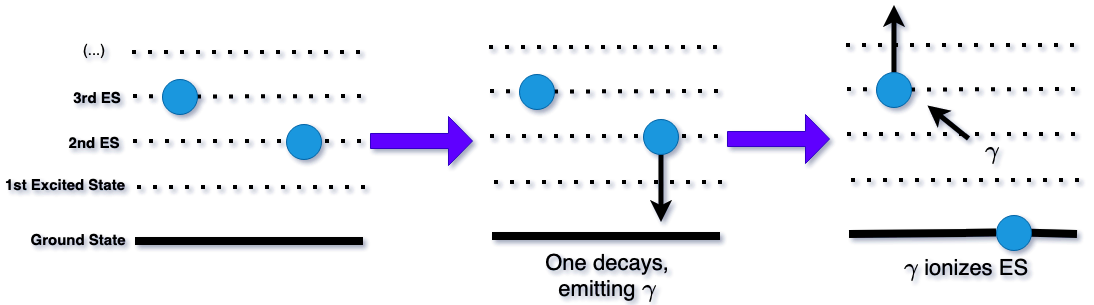
Figure 1: Ion particles ionization and de-excitation in a CR model.

These include the species ion charge state distribution $n_{\alpha,Z}$ and the radiative cooling rate $\mathcal{R}_{L}$. The species charge state density $n_{\alpha,Z}$ is simply the sum over all ground and excited states of a given charge state,

$$n_{\alpha,Z}=\sum_{j}N^{j}_{\alpha,Z}.$$

The radiative power loss (RPL) rate is a crucial quantity chracterizing the radiative cooling rate of electrons in a plasma. It can be calculated by summing up the contributions from all radiative transitions, including line emissions (bound-bound), recombination radiation (free-bound), and bremsstrahlung (free-free). As an example, the line emission rate takes the form:

$$\mathcal{R}_{L}=\sum_{\alpha,Z,j,k}N_{\alpha,Z}^{j}A^{j}_{\alpha,Z\rightarrow k}E^{j}_{\alpha,Z\rightarrow k},$$

where $A^{j}_{\alpha,Z\rightarrow k}$ is the coefficient for spontaneous emission from energy level $j$ to level $k$, and $E^{j}_{\alpha,Z\rightarrow k}$ is the the energy of the photon emitted in the transition from level $j$ to level $k$.

The CR model is mathematically represented as a parameterized ODE:

$$\frac{d\mathbf{N}}{dt}={R}(\mathbf{N};n_{A},T_{e})\,\mathbf{N},$$ (1)

where $\mathbf{N}$ is the population density vector of ions in various charge states including both ground and excites states, $T_{e}$ is the temperature, $n_{A,\alpha}=\sum_{Z}n_{\alpha,Z}$ is the total atomic density for species $\alpha$. The dimension of $\mathbf{N}$ can vary enormously depending on whether one would want to resolve the fine and super-fine structures in the excited states. As an example, LANL’s ATOMIC model [[][]hakel2006new] can have more than $10^{6}$ states for argon. The rate matrix ${R}(\mathbf{N};n_{A},T_{e})$ is a square matrix describing a range of atomic processes, which can be broadly grouped in up-transitions and down-transitions. The up-transitions include electron impact ionization/excitation, photo-ionization and excitation. The down-transitions account for various channels of recombination and de-excitation. Collisional charge exchange can provide both down- and up-transitions depending on the specific ion/atom involved. The overall rate matrix ${R}$ has explicit dependence on the electron distribution. The normal assumption is to approximate the electron distribution as a Maxwellian with temperature $T_{e}$ and density $n_{e}.$ In a quasineutral plasma, the electron density is approximately equal to ion charge density $\sum_{Z,\alpha}Zn_{\alpha,Z}.$ The species atomic number density $n_{\alpha}$ or more explicitly labeled as $n_{A,\alpha},$ is the sum of all charge states $\sum_{Z}n_{\alpha,Z}.$ for species $\alpha$.

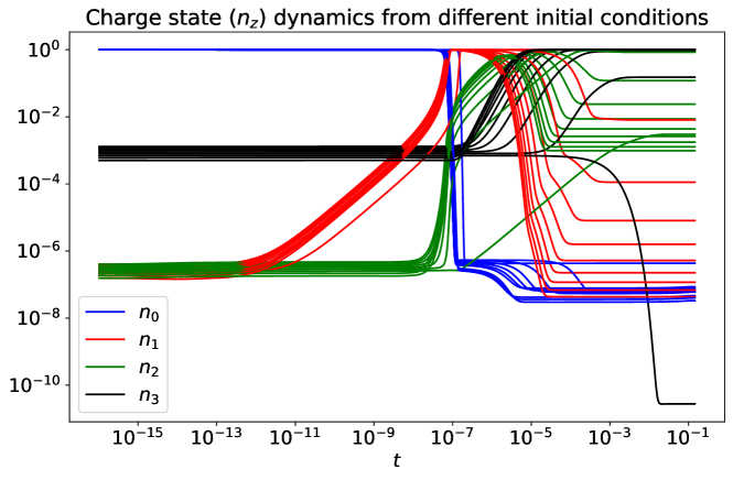
Figure 2: Trajectory of the charge state from the high-fidelity numerical simulation of the CR model for different initial conditions. The solution is for a single species, lithium, where the atomic number $A_{\alpha}=3$. Four colored lines represent four charge states (they are partial sums of the solution state vector; details will be defined later), $n_{0},n_{1},n_{2},n_{3}$.

The CR model is a set of parameterized stiff ODE, as many of the transition rates are very fast compared with the time scale for reaching ionization balance. Numerical solutions of the full system (1) require implicit time stepping which is usually performed along with a standard linear algebra package. Resolving the CR model can be a computational burden for potentially the millions of degrees of freedom in $\mathbf{N},$ in which case it would be simply impossible to couple the CR physics module in its native form with 3D plasma simulations, since for each spatial grid point in the plasma simulation, one would need to evolve a coupled ODE with many degrees of freedom, which would overwhelm the plasma simulation cost by many orders of magnitude. The goal of this work is to introduce a reduced-order model that can efficiently and accurately predict the fast dynamical transition of the charge state, $n_{\alpha,Z}$, and the radiative cooling rate, $\mathcal{R}_{L}$.

I.2 Related Work

Reduced Order Modeling (ROM) seeks low-dimensional approximations of high-dimensional systems, in order to significantly reduce computational costs. In the framework of data-driven ROM, machine learning (ML) techniques and data are used to distill the essential features of complex systems into more manageable representations. This is especially relevant in fields such as fluid dynamics, material science, and climate modeling, where solving full-scale problems involves significant computational challenges due to high dimensionality. Proper Orthogonal Decomposition (POD) and Dynamic Mode Decomposition (DMD) are two of the most popular approaches to extract dominant features and dynamic structures from data. These methods have been successfully applied in fluid mechanics, control, and biomechanical problems [[][]xie2018data, xie2017approximate, amsallem2012stabilization, snyder2023numerical, peherstorfer2015dynamic]. With the development of deep learning, autoencoder neural networks have gained significant attention in ROM due to their ability to efficiently compress high-dimensional data into a lower-dimensional latent space while preserving essential features. Recent works have demonstrated the use of autoencoders for learning low-dimensional representations of fluid dynamics [[][]mardt2018vampnets, hasegawa2020machine]. Ref. [[][]champion2019data] combined autoencoders with DMD to learn the governing equations of dynamical systems directly from data, allowing for efficient predictions of future states.

Data-driven discovery of dynamics has emerged as a powerful tool for modeling and predicting the behavior of complex physical systems. This approach leverages ML techniques to extract patterns and underlying dynamics from data, facilitating the development of reduced-order models that are both efficient and accurate. Ref. [[][]brunton2016discovering] introduced the Sparse Identification of Nonlinear Dynamical Systems (SINDy) method, which aims to discover governing equations from data. By representing the dynamics in a library of candidate functions, SINDy selects the most relevant terms to construct a parsimonious model. This data-driven methodology has proven effective in capturing the underlying physics of complex systems with minimal assumptions, offering a powerful tool for system identification and model reduction [[][]fukami2021sparse, kaheman2020sindy]. Ref. [[][]chen2018neural] introduced Neural Ordinary Differential Equations (NODE), which parametrize the time derivative of the hidden state with a neural network, allowing the model to learn complex dynamics directly from data. This method can also be applied for identifying latent dynamics [[][]rubanova2019latent, linot2023stabilized]. Ref. [[][]lusch2018deep] utilized autoencoders to identify a latent space where the nonlinear dynamics are approximated by linear models based on linear Koopman operator theory, enabling efficient and accurate predictions of system behavior. Ref. [[][]koronaki2024nonlinear] introduced physics- and data-assisted ROM based on approximate inertial manifolds theory using deep neural networks. Their approach is successfully demonstrated through dissipative PDEs. Ref. [[][]koronaki2024nonlinear] discussed the “physics-assisted” latent space learning where the latent space is a “grey-box” approach including the known physics latent space and data-driven latent space. A few recent works on learning flow maps using structure-preserving neural networks can be found in [[][]burby2020fast, duruisseaux2023approximation], which has been recently applied to learning beam dynamics in accelerators [[][]huang2024symplectic]. These studies underscore the potential of integrating ROM approach with latent dynamics learning to address the computational challenges in simulating high-dimensional dynamical systems.

I.3 Specific aim and approach of this work

The main challenge in finding the reduced CR model for coupling to plasma simulations lies in two parts. The first is to efficiently identify the low-dimensional representation from the data. The second is to learn latent dynamics that can accurately predict the trajectories of the reduced system using only the initial conditions. This allows for an approximation of the full-order dynamics and the radiative cooling rate with high accuracy. Fig. 2 plots the trajectories of different charge states from the high-fidelity numerical simulation. It is evident that the sharp transitions over very short time scales present a significant challenge in accurately modeling the reduced CR dynamics.

It should be emphasized that for the purpose of coupling the surrogate CR model to plasma simulations, the two essential quantities, which are of explicit physics meaning, are the species ion charge state density $n_{\alpha,Z}(t)$ and the radiative power loss (RPL) rate $\mathcal{R}_{L}(t).$ The first will enter the plasma model to update the ion charge distribution, while the second will enter the plasma model as an energy sink term for the electron thermal energy. Since we have decided to evolve a surrogate model in a much lower dimensional latent space to save computational cost in coupled CR-plasma simulations, it becomes a necessity to include the physical variables $n_{\alpha,Z}$ in the latent space. This naturally leads to a grey box latent space in which physical variables in the white space and the usual blackbox variables that have no physical meaning, would co-reside. So the actual latent space discovery, which refers to the unknown black space variables, is constrained by the required presence of white space variables for the decoder network and its training. In other words, the deployment of white space variable in the grey box latent space is required to facilitate the coupling of the latent space surrogate model to plasma simulations. It is unclear, or at least we do not know, if the presence of these white space variables is actually beneficial to extract a more optimal black subspace, in terms of both the training cost for the encoder-decoder and the minimal size of the latent space. For potential benefit of “physics-assisted” as opposed to “physics-constrained” latent space discovery reported here, one can consult Ref. [[][]koronaki2024nonlinear].

Consistent with the need of direct coupling to the plasma simulation model, the radiative power loss rate $\mathcal{R}_{L}$ will be reconstructed with the decoder, in addition to the full vector of $\mathbf{N}.$ The CR time dynamics, from the data, is given by $\mathbf{N}(t_{n})$ at discrete time $t_{n},$ with a variable time step $\Delta t_{n}=t_{n+1}-t_{n}.$ The corresponding latent space dynamics is modeled by a flow-map neutral netwrrk, which is a common approach for learning discrete dynamical system [[][]rnn, lstm]. It is interesting to note that the extreme variation in $\Delta t_{n}$ makes our dynamical surrogate reconstruction a standout among those flow-map NN work reported in the literature. For the purpose of demonstration, our approach will be tested by the CR data from a single species, lithium, under different parameters and initial conditions in Section III.

II Data-Driven Model Reduction for CR modeling

This section describes the deep learning approach for our latent space model reduction of the CR data. The methodology involves two crucial steps: latent space discovery (reduction) and latent dynamics learning, both of which are facilitated by designing an appropriate neural network architecture. The network comprises an encoder to reduce the input high dimensional data into a lower-dimension latent space, followed by a neural network to learn the flow map of the latent space dynamics. Subsequently, a decoder is employed to reconstruct the full ion density space and radiative power loss rate $\mathcal{R}_{L}.$ Fig. 3 illustrates the architecture of our data-driven ML-based surrogate for the CR system.

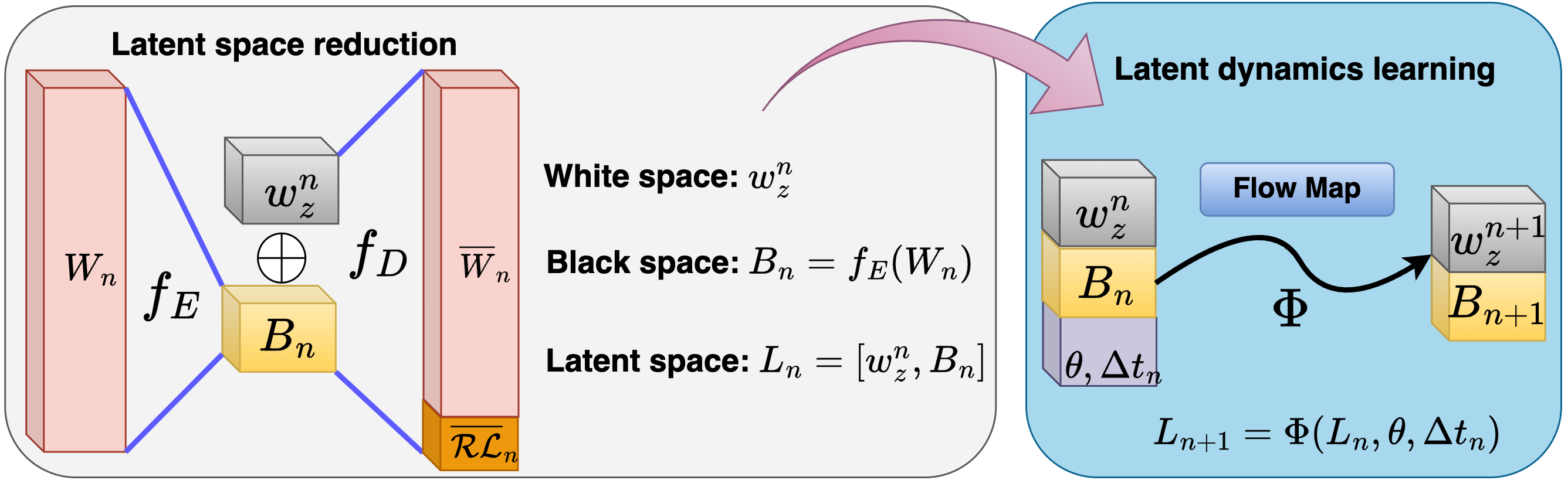
Figure 3: Autoencoder architecture for physics-assisted latent space identification (left). Flow map for latent dynamics learning (right). $\theta$ denotes the parameter space in our CR system which are total density, $n_{A}$, and temperature, $T_{e}$.

II.1 Grey Latent Space Discovery via Autoencoder

For latent space discovery, we are constrained that there needs to be a white subspace for explicitly tracking the ion charge state distribution $n_{\alpha,Z}$ to couple the surrogate CR model with plasma simulations. The autoencoder is thus primarily to discover the minimal size of the black subspace. This black subspace has the critical role of improving the ionization balance and radiative loss rate beyond the usual coronal equilibrium approximation, which only tracks the ground states of ions/neutrals.

Autoencoders consist of two main components: an encoder function $f_{E}$, which maps the input data to a lower-dimensional latent space, and a decoder function $f_{D}$, which reconstructs the original data from its latent representation. During the training, the autoencoder minimizes the reconstruction error between the input and the reconstructed output, thereby capturing the most significant features of the data. In the first part of our data-driven framework, an autoencoder is utilized to reduce the full ion population space into a black space, $B_{n}$, at a given time step $t_{n}$. The black space in combination with the known physics information of the charge state (i.e., a white space, $w_{z}^{n}$) forms our latent space, $L_{n}$. The full ion population can then be reconstructed through a decoder $f_{D}$ from this latent space. Note that when setting the dimension of the black space to zero, we recover the charge states as our latent space, which would be the limit of a time-dependent coronal equilibrium model. This is usually too crude a reduction to recover accurately the radiative power loss rate $\mathcal{R}_{L},$ which we shall retrieve from the decoder, through a finite-sized black subspace in the autoencoder latent space. In our case, the encoder part transforms the input, i.e., a normalized ion population $W_{n}\in\mathbb{R}^{n}$, to a black space $B_{n}\in\mathbb{R}^{r}$ with $r\ll N$:

$$B_{n}=f_{E}(W_{n}).$$

The decoder part tries to reconstruct the input $W_{n}$ and predict the radiative loss from the latent space $L_{n}=[w_{z}^{n},B_{n}]$:

$$[\overline{W_{n}},\overline{\mathcal{R}_{L,n}}]=f_{D}(L_{n}).$$

The objective is to minimize the reconstruction loss $\mathcal{L}_{recons}$, which measures the difference between the input $W_{n}$ and the reconstructed output $\overline{W_{n}}$ and $\overline{\mathcal{R}_{L,n}}$:

$$\mathcal{L}_{\rm recons}=\frac{1}{S}\sum_{n=1}^{S}\Big{[}\|W_{n}-\overline{W_{n}}\|^{2}+\|\mathcal{R}_{L,n}-\overline{\mathcal{R}_{L,n}}\|^{2}\Big{]},$$

where $S$ is the total number of time steps in our training dataset.

II.2 Latent Dynamics Learning via Flow Maps

A dynamical CR model is formally a continuous-time dynamical systems described by ordinary differential equations (ODEs). Its latent system’s behavior can be expressed as:

$$\frac{d\mathbf{L}}{dt}=\mathbf{F}(\mathbf{L;\theta}),$$

Here, $\mathbf{L}\in\mathbb{R}^{r}$ is the reduced latent state vector, and $\mathbf{F}(\mathbf{L};\theta)$ is the vector field that describes the dynamics of the system parameterized by $\theta$. One can construct such a system and pursue a neural ODE integration scheme for coupling the surrogate CR model to plasma simulation.

In this work, we opt to construct a surrogate CR model in the form of a discrete-time flow map from $t$ to $t+\Delta t,$ which describes the time integration of the ODE system over discrete time steps. The flow map $\Phi(\Delta t,\mathbf{L}_{0})$, is a function that maps the initial state $\mathbf{L}_{0}$ at $t=t_{0}$ to its future state $\mathbf{L}(t)$ at a time interval $\Delta t$, such that:

$$\mathbf{L}(t_{0}+\Delta t)=\Phi(\Delta t,\mathbf{L}(t_{0}))$$

This discrete-time flow map arises naturally in coupling the CR model with plasma simulations using a finite step size $\Delta t$ in time integration. In general, for discrete-time dynamical systems with a uniform time step, the system can often be described by:

$$\mathbf{L}_{n+1}=\mathbf{G}(\mathbf{L}_{n}).$$

Since time integration of our CR model has exponentially varying time steps and is also parameterized by the total density $n_{A}$ and temperature $T_{e}$, our flow map $\Phi$ acts at discrete steps, mapping $\mathbf{L}_{n}$ to $\mathbf{L}_{n+1}$ and can be denoted as:

$$\mathbf{L}_{n+1}=\Phi(\Delta t_{n},\mathbf{L}_{n};n_{A},T_{e}),$$

see the Fig. 3 for the model architecture. In this case $\theta$ includes $n_{A}$ and $T_{e}$. Thus, the flow map can be approximated by a neural network with the loss function defined as the following,

$$\mathcal{L}=\frac{1}{S}\sum_{n=0}^{S}\Big{[}\|\mathbf{L}_{n+1}-\Phi(\Delta t_{n},\mathbf{L}_{n};\theta)\|^{2}+\|n_{A}-\sum_{i=0}^{Z}n^{n+1}_{i}\|^{2}\Big{]},$$

where $\Phi(\Delta t_{n},\mathbf{L}_{n};\theta)$ is the neural network prediction of the trajectory at next time step, and $\|n_{A}-\sum_{i=0}^{Z}n^{n+1}_{i}\|^{2}$ is the additional physical constraint, i.e., the mass conservation of atomic species.

III Numerical Experiment

In this section, we present detailed numerical experiments for the proposed surrogate model in Section II. The case study is performed with a single atomic species of lithium, using a superconfiguration atomic model and the rates from the FLYCHK code [[][]chung2005flychk]. The CR solution of Lithium has $\dim{\mathbf{N}}=94$ states corresponding to different energy levels. Since the atomic number $A_{\alpha}=3$, we have 4 charge states defined as the following,

$$n_{0}:=\sum_{i=0}^{31}N_{i},\qquad n_{1}:=\sum_{i=32}^{62}N_{i},\qquad n_{2}:=\sum_{i=63}^{93}N_{i},\qquad n_{3}:=N_{94}.$$

Fig. 2 shows the charge state trajectories from different initial conditions from the high-fidelity CR model. We can clearly see that there is sharp transition at very tiny time scale in the CR dynamics, which makes it one of many challenges in the reduced latent dynamics learning.

III.1 Data processing

The success of the ML training heavily relies on the proper data processing. Here we describe two critical components to rescale the data to ease the ML training. A proper sampling for stiff dynamics is also an important step to guarantee a good training result.

Ion Density Normalization.

The magnitude of ion population $\mathbf{N}$ from the numerical solution varies largely between 1e13 to 1e-11. Since the total density $n_{A}$ should be preserved for different parameter setting, we first normalize the population using its total density $n_{A}$ as the follows,

$$\tilde{\mathbf{N}}=\frac{\mathbf{N}}{n_{A}},\qquad n_{A}=\sum_{z=0}^{Z}n_{z}$$

After the total density scaling, the range of ion population density $\tilde{\mathbf{N}}$ lies in $($1e-27$,1)$. Many of the ion densities are still very small, with magnitudes less than 1e-10, making it challenging for the neural network to learn such values of tiny magnitude. To accurately resolve the high-fidelity dynamics of the CR model, it is important to resolve small values of the states, Fig. 4 shows the high-fidelity solution of the charge state dynamics from different temperature $T_{e}$. The raw data however is dominated by one or two states that have much larger magnitudes.

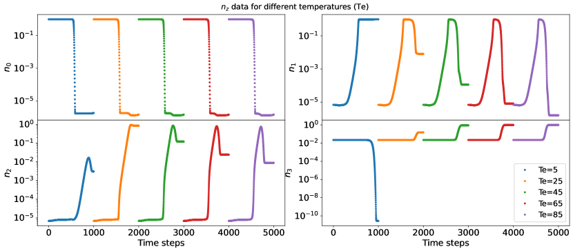
Figure 4: High fidelity CR solution of charge state $n_{z}$. Trajectories from 10 different temperatures $T_{e}$ are plotted.

To accommodate that, we first apply the following change of variable to transform the data into a more suitable range:

$$\tilde{W}={1-\log(\tilde{\mathbf{N}})},$$

then using $(0,1)$ min-max scaler on $\tilde{W}$ to obtain the properly scaled training data $W$:

$$W=\frac{\tilde{W}-\tilde{W}_{min}}{\tilde{W}_{max}-\tilde{W}_{min}}.$$

The transformed variable $W$ lies in $(0,1)$ and is properly scaled, making it easier for the neural network to train effectively. Fig. 5 shows the charge state, $n_{z}$, both in its original scale and its normalized scale (between 0 and 1), as used in practical neural network training. Note that we use the notation $w_{z}$ (w0, w1, w2, w3) to represent the transformed charge state of $n_{z}$ (n0, n1, n2, n3).

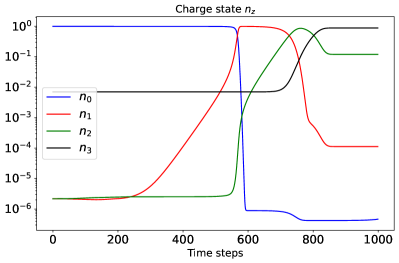
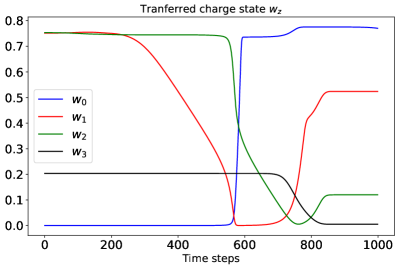
Figure 5: Charge states in the original scale, $n_{z}$, and in the normalized scale, $w_{z}$. The latter is used in the neural network training.

Time Step Scaling.

Time step size scaling is another crucial aspect for a successful training. For stiff equations or rapidly changing dynamics, a fixed time step size is often inadequate for capturing the system’s behavior accurately. In such cases, adaptive time stepping methods, based on the local behavior of the system, are employed. This adaptive approach often results in more accurate and computationally efficient simulations. In the high-fidelity numerical simulation of the CR model, we used prescribed adaptive time steps in the numerical integration. The dataset was collected from non-uniform time step solutions with $\Delta t_{n}$ ranging from $10^{-16}$ to $10^{-1}$. The tiny scale of the time step size makes it challenging to train the neural network, as we input $\Delta t_{n}$ into the flow map to learn the latent dynamics evolution from current step $L(t_{n}$) to the next $L(t_{n+1})$. To make the neural network training more efficient, we use the following transfer formula to scale $\Delta t_{n}$ into a proper range of $(0,1)$,

$$\tilde{\Delta t}=-\frac{1}{\log(\Delta t)}.$$ (2)

See Fig. 6 for a demonstration.

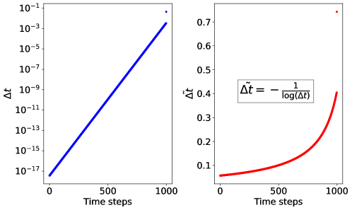
Figure 6: Scaling of the time steps.

Resampling.

We simulate the CR equation (1) with 37 temperatures $T_{e}$ from 5eV to 95eV with a step size of 2.5, 10 different total densities with $n_{A}=$[1e14, 2e14, 3e14, 4e14, 5e14, 6e14, 7e14, 8e14, 9e14, 1e15], and 40 different initial conditions. This results in a total of 14,800 trajectories. The dataset was collected with 1,000 time steps for each trajectory, leading to 14.8 million pairs of $(L_{n},L_{n+1})$ in the flow map neural network training to learn latent dynamics. This large dataset is very expensive to train in practice. Additionally, there are a significant number of tiny time steps in each run, of which the corresponding flow maps are near-identity mappings (the first 500 time steps). This poses two challenges: first, the dataset size is substantial, and second, the presence of many near-identity mappings makes the training process difficult. To address these issues, we performed coarse sampling of the data. The purposes of this approach were to reduce the dataset size and to avoid the identity mappings. Instead of using all 1,000 time step data points, we performed coarse sampling to retain 161 points; see Fig. 7. Note that time steps are selected to fully resolve the sharp transition of the dynamics.

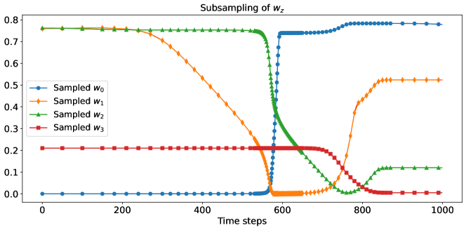
Figure 7: Resampled data points from the true trajectory.

III.2 Autoencoder Training

The entire model is trained in two steps. First, we train the autoencoder to identify the latent space. Next, we use a flow map neural network (FMNet) to learn the latent dynamics. In the autoencoder architecture, the encoder and decoder both have two hidden layers. The input is the normalized ion population density $\mathbf{W}$ with an input dimension of 94. The output of the decoder is the reconstruction of the ion population density and radiative loss rate $\mathcal{R}_{L}$, with a dimension of 95. Increasing the number of hidden neurons and the latent space size increases the training cost. For the fully connected layers, sigmoid activations are used. The learning rate has constant decay after every 1000 epochs starting with $0.001$. We trained the model for 10,000 epochs, experimenting with different numbers of hidden units and latent space dimensions. To balance accuracy and efficiency, using $h1=64,\,h2=32$, and a latent space of dimension 10 (it consists of a black space of dimension 6 and the white space of dimension 4) provides a reasonably accurate reconstruction and prediction of radiative loss. Fig. 8 shows the autoencoder architecture. Fig. 9 shows the representative prediction of $\mathcal{R}_{L}$ from the decoder. The model is trained using one NVIDIA A100 GPU. Under this configuration, the training cost is 27 hours. We used this latent space configuration for our flow map training.

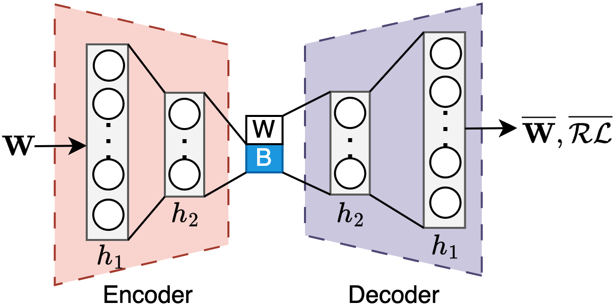
Figure 8: The autoencoder architecture, $h_{1},h_{2}$ are the hidden layers with units 64 and 32 respectively

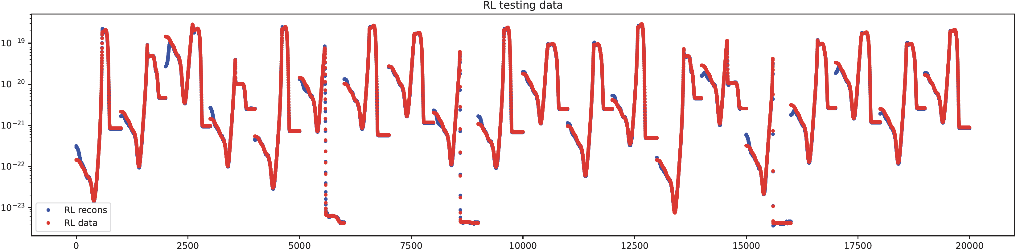
Figure 9: The radiative loss rate $\mathcal{R}_{L}$ prediction from the autoencoder neural network. The radiaitive loss prediction for 20 trajectories are plotted. Red points are the true data, blue dots are the prediction from the decoder

III.3 Flow Map Training

III.3.1 Prediction Error

In the prediction phase, we provide the initial condition (latent variable at $t_{0}$ projected by the encoder) to the FMNet. FMNet then iteratively predicts the latent trajectory, which includes both the charge state dynamics (white space) and the unknown dynamics (black space); see Fig. 10. This latent trajectory is subsequently fed into the decoder to obtain the radiative loss rate $\mathcal{R}_{L}$. The prediction error of the charge state, used in our model evaluation, is defined as the Mean Squared Error (MSE) at each time step,

$$e_{pred}=\frac{1}{S}\sum_{i=1}^{S}\|n^{i}_{z}-\overline{n^{i}_{z}}\|^{2}$$

It is important to note that the training error is computed based on one-step predictions, while the prediction error in the testing phase accumulates at every time step, reflecting the compound effect of iterative predictions. Using prediction errors to evaluate model performance ensures the robustness and reliability of the model, making it suitable for practical applications in predicting radiative loss rates and understanding charge state dynamics. By leveraging the latent space representation, the reduced-order model effectively reduces computational complexity while maintaining high accuracy. This approach facilitates efficient and accurate simulations in high-fidelity numerical experiments, thereby enhancing the model’s utility in real-world scenarios.

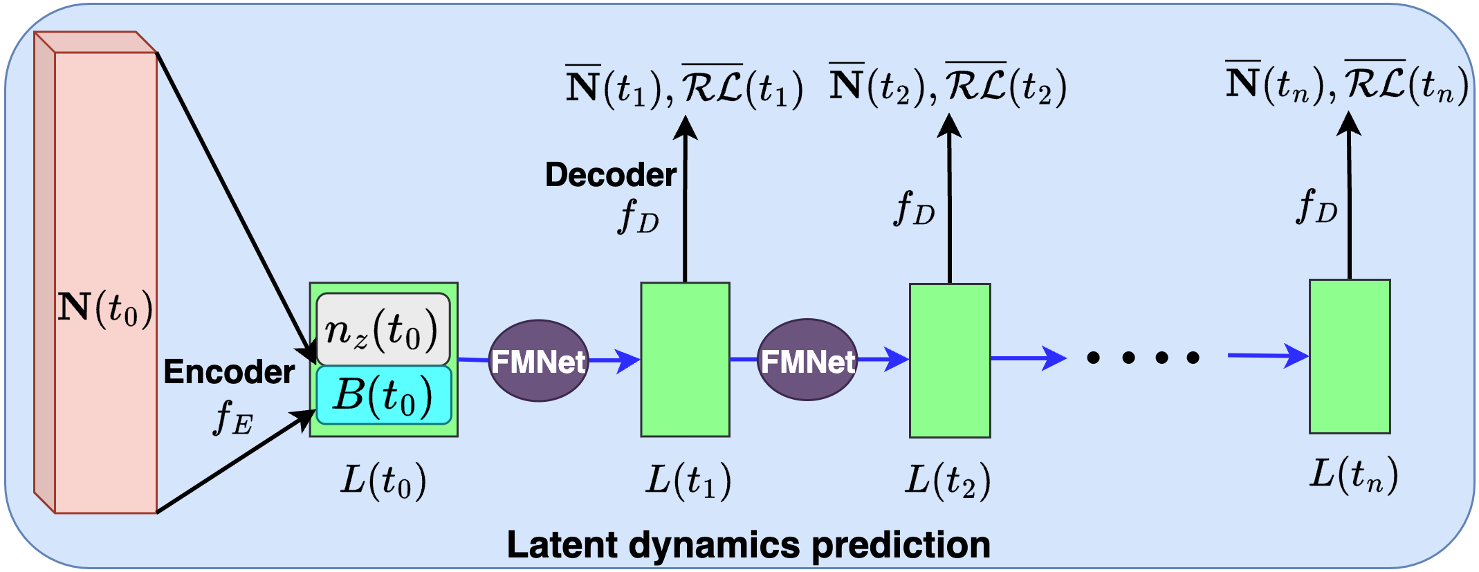
Figure 10: The iterative prediction scheme of the latent dynamics and radiative loss rate $\mathcal{R}_{L}$ after the autoencoder and flow map network (FMNet) are trained.

III.3.2 Dynamics Prediction from Different Initial Conditions

We first evaluate the performance of the FMNet under various initial conditions. We initialize the FMNet with different latent variables, each corresponding to a unique initial condition in the high-fidelity simulation data. The purpose of this evaluation is to assess the model’s ability to generalize and accurately predict the CR dynamics from different starting points. We select a representative set of initial conditions that span the range of typical operating conditions for the CR model. For each initial condition, the FMNet iteratively predicts the latent trajectory, capturing the evolution of charge state dynamics and unknown dynamics. The predicted latent trajectories are then decoded to obtain the corresponding radiative loss rates $\mathcal{R}_{L}$. We quantify the prediction accuracy using metrics such as Mean Squared Error (MSE) and Mean Absolute Error (MAE) across all time steps for each initial condition. The results are compared to the ground truth obtained from the high-fidelity simulations. Fig. 11 illustrates the prediction performance for a subset of initial conditions, showing both the predicted and true trajectories of key variables. Fig. 12 shows the corresponding radiative loss predictions. Our result indicates that the model maintains robust performance across a wide range of initial conditions, with prediction errors remaining within acceptable bounds. This demonstrates the model’s capability to adapt to different starting points and accurately capture its dynamics.

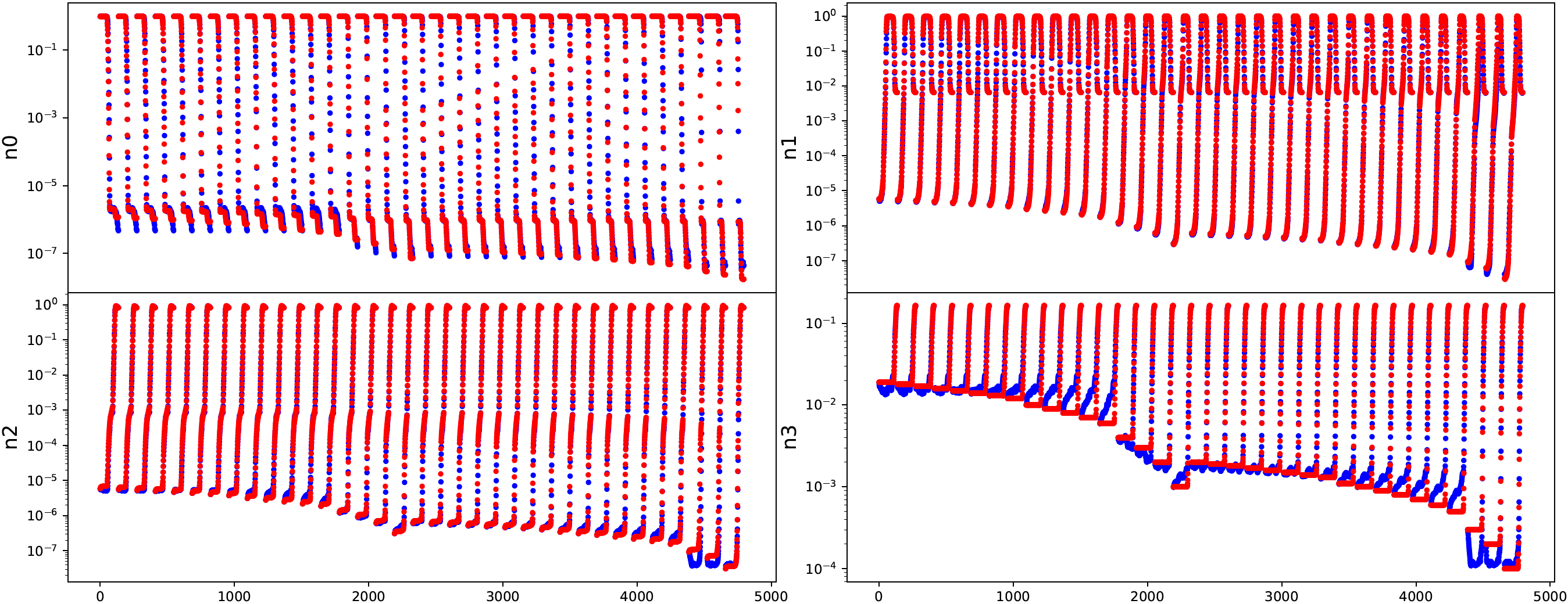
Figure 11: Charge state $n_{z}$ trajectory prediction from the flow map neural network (FMNet). Each trajectory represent different initial conditions. Red dots are the true data, and blue dots are the FMNet prediction

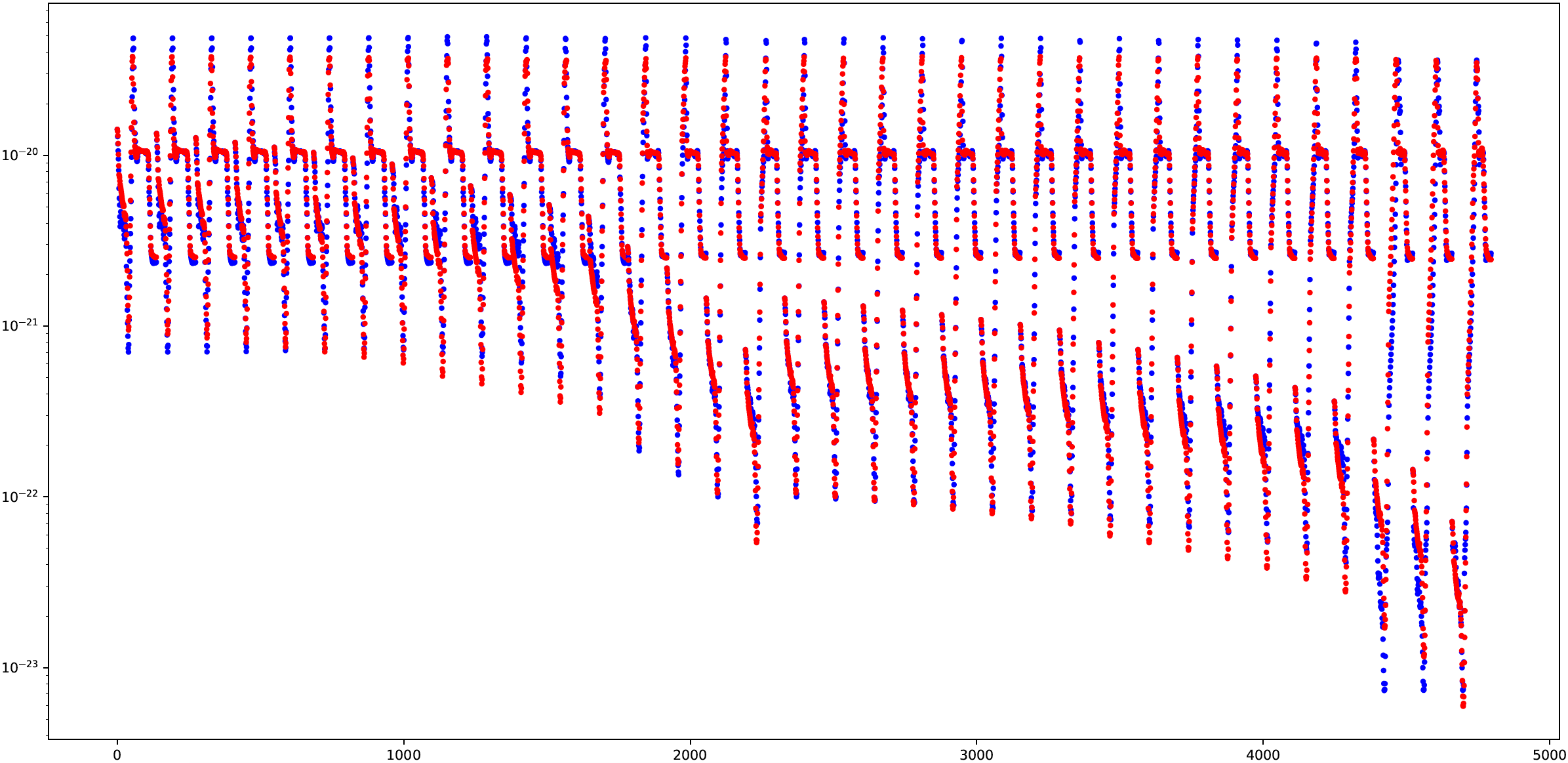
Figure 12: Radiative loss rate prediction from the decoder after feeding the predicted latent dynamics.

III.3.3 Dynamics Prediction from Different Parameters

In this section, we extend the evaluation to different parameter settings for total density $n_{A}$ and electron temperature $T_{e}$. These parameters play a crucial role in the behavior of the CR model, influencing the rates of collisional and radiative processes. To assess the model’s performance across different parameter values, we generate predictions for various combinations of $n_{A}$ and $T_{e}$. The FMNet is trained to account for these parameters as inputs, enabling it to adapt its predictions based on the specific conditions. We systematically vary $n_{A}$ and $T_{e}$ within their respective ranges used in the high-fidelity simulations, Fig. 13 shows the split of the parameters in dataset for training, validation and testing. For each combination of $n_{A}$ and $T_{e}$, the model predicts the latent trajectory and the corresponding radiative loss. We then compare these predictions to the ground truth data, using prediction error. Figs. 14 and 15 show the prediction results charge state and radiative loss. These plots illustrate the model’s ability to accurately capture the dynamics under varying conditions. Our findings suggest that the model performs well across a broad spectrum of parameter values, maintaining high accuracy in its predictions. This highlights the model’s flexibility and robustness, making it a valuable tool for simulating and understanding the behavior of the CR system under different physical conditions.

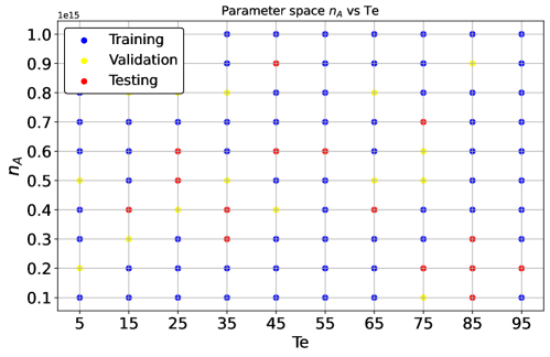
Figure 13: Parameters sampled for training and prediction test.

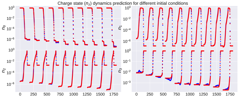
Figure 14: Charge state trajectory prediction at temperature $T_{e}=65$, $n_{A}=$5e14 with different initial conditions in the testing dataset, 10 trajectories are plotted. Red represents true data, and blue represents the model prediction.

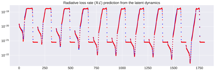
Figure 15: Radiative loss rate prediction at temperature $T_{e}=65$, $n_{A}=$5e14 with different initial conditions in the testing dataset. Red represents true data, and blue represents the model prediction.

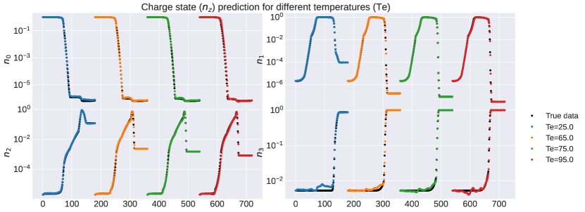
Figure 16: Charge state trajectory prediction for different temperatures $T_{e}$ in the testing dataset. Red represents true data, and 4 different colors represent the model prediction from different temperatures.

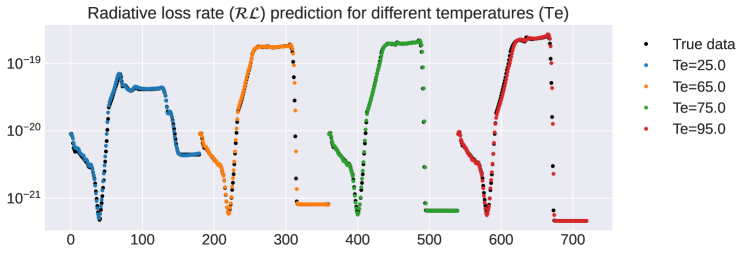
Figure 17: Radiative loss rate prediction for different temperatures $T_{e}$ in the testing dataset. Red represents true data, and 4 different colors represent the model prediction from different temperatures.

III.3.4 Neural Network Architecture Search

Neural network architecture search (NAS) is a crucial process in the development of ML models, focusing on automating the design of optimal neural network architectures. The idea behind NAS is to systematically explore a vast search space of possible architectures to identify the most effective configurations that meet specific performance criteria, such as accuracy, efficiency, and computational cost.

In practice, NAS involves defining a search space that specifies the range of possible architectures, including the number of layers, the type of layers (e.g., convolutional, fully connected), and the number of units in each layer. The search algorithm then navigates this space to find architectures that maximize a given performance metric on a validation dataset. In our work, we employed a grid search methodology to systematically explore a range of possible configurations. The primary objective was to determine the optimal architecture by varying the number of layers and the number of hidden units within each layer. The number of layers range set was from 2 to 7 layers. This range includes both simpler models with fewer layers, which may train faster and are less prone to overfitting, and more complex models with additional layers, which have the capacity to capture more intricate patterns in the data. For each layer, the number of hidden units was varied between 16 and 512. By systematically combining these two parameters (number of layers and hidden units), the grid search examined a wide array of architectures and it gives an initial study on the optimal neural network structure for our training data. The results show that the FMNet nearly reaches its best prediction error with 3 layers and 256 units for each layer; see Fig. 19.

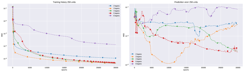
Figure 18: Training history of the FMNet. Training error (left) vs prediction error (right) from different network architectures.

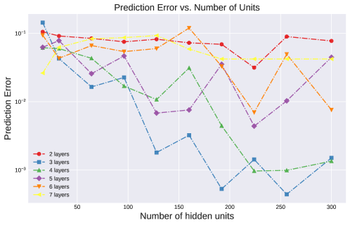
Figure 19: Prediction error from models with different architecture. The FMNet reaches its best prediction error with 3 layers and 256 units for each layer.

Addressing NAS effectively requires balancing the exploration of diverse architectures with the exploitation of promising configurations. Techniques such as early stopping, weight sharing, and transfer learning are often employed to reduce the computational burden and accelerate the search process. As NAS continues to evolve, it holds the potential to significantly advance the field of neural network design, making it more accessible and efficient. The grid search we used in this study is computationally expensive and may miss optimal configurations lying between grid points. In the future work, we will explore Bayesian optimization and reinforcement learning for more robust search.

III.3.5 Impact of Training Data Size

The performance of neural networks is influenced by two key factors: the amount of training data available and the complexity of the model architecture. In the previous section, we used a grid search method to find the optimal neural network architecture. In this section, we explore how increasing the size of the training dataset and the complexity of the neural network model impacts prediction performance.

One of the fundamental principles in ML is that larger datasets tend to produce better models. When training a neural network on a small dataset, the model may not have enough examples to learn robust patterns and relationships in the data. As a result, the model may suffer from overfitting, where it memorizes the training data rather than generalizing well to unseen data. By increasing the size of the training dataset, we provide the model with more diverse examples to learn from, which can help improve its ability to generalize. As the amount of training data increases, the model becomes more exposed to different variations and nuances present in the data, allowing it to learn more robust representations. Consequently, we typically observe better prediction performance as the size of the training dataset grows. Since our dataset is parameterized by the $n_{A}$ and $T_{e}$, we use $T_{e}$ as the benchmark to test the impact of the datasize. We split the dataset according to the $T_{e}$ values. For the testing dataset, we use $T_{e}=$[15, 45, 75, 95]. Our initial training only contains data with $T_{e}=$[5, 25, 35, 55, 65, 85] (black dots in Fig. 20). The second training we use the full dataset (blue dots in Fig. 20). The results clearly indicate that increasing the training dataset can lead to better prediction performance for the model, as demonstrated in Figs. 21 and 22.

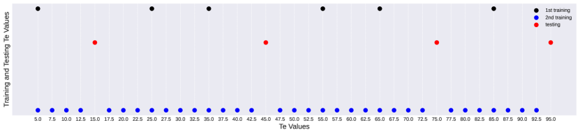
Figure 20: Data used for different training test

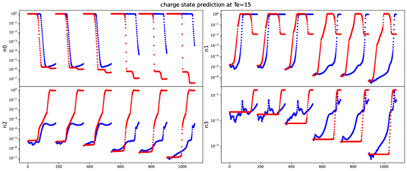
Figure 21: Charge state prediction from the FMNet trained with first training $T_{e}$ data (see dark dots in Fig. 20).

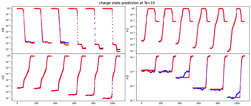
Figure 22: Charge state prediction from the FMNet trained with full $T_{e}$ values data.

IV Conclusion and Future Work

In this paper, we have introduced a physics-assisted surrogate model framework tailored for Collisional-radiative (CR) modeling. Our approach leverages a mixed latent space, comprising a “white space” that provides the physical variables for coupling with the plasma models, and a “black space” discovered through an autoencoder to ensure accuracy. Subsequently, neural networks are utilized to learn the dynamics governing this latent space. In the numerical experiments, by thoroughly evaluating the model’s performance under various initial conditions and parameter settings, we demonstrate its reliability and effectiveness in predicting the complex dynamics of the CR model. This comprehensive analysis provides confidence in the model’s applicability to real-world scenarios, where accurate and efficient predictions are essential for understanding and mitigating plasma disruptions in fusion reactors. The presented numerical results substantiate the effectiveness of our approach, demonstrating promising accuracy in modeling the CR problem.

In future work, we plan to expand our model to include data from multiple species. Incorporating a broader range of species will enhance the model’s applicability and robustness, allowing for more comprehensive predictions of radiative loss rates and charge state dynamics across different plasma conditions. This expansion will inevitably increase the dataset size and complexity, presenting new challenges in terms of computational requirements and training costs which we will use distributed training with multiple GPUs. Additionally, we aim to integrate NODEs into our framework. NODEs offer a powerful approach for modeling continuous-time dynamics, allowing the model to learn the system’s evolution directly from data.

References

- [1] Nathan A Garland, Hyun-Kyung Chung, Christopher J Fontes, Mark C Zammit, James Colgan, Todd Elder, Christopher J McDevitt, Timothy M Wildey, and Xian-Zhu Tang. Impact of a minority relativistic electron tail interacting with a thermal plasma containing high-atomic-number impurities. Physics of Plasmas, 27(4), 2020.
- [2] Nathan A Garland, Romit Maulik, Qi Tang, Xian-Zhu Tang, and Prasanna Balaprakash. Progress towards high fidelity collisional-radiative model surrogates for rapid in-situ evaluation. In Third Workshop on Machine Learning and the Physical Sciences (NeurIPS 2020)(Vancouver, Canada), 2020.
- [3] Nathan A Garland, Romit Maulik, Qi Tang, Xian-Zhu Tang, and Prasanna Balaprakash. Efficient data acquisition and training of collisional-radiative model artificial neural network surrogates through adaptive parameter space sampling. Machine learning: science and technology, 3(4):045003, 2022.
- [4] P Hakel, ME Sherrill, S Mazevet, J Abdallah Jr, J Colgan, DP Kilcrease, NH Magee, CJ Fontes, and HL Zhang. The new Los Alamos opacity code ATOMIC. Journal of Quantitative Spectroscopy and Radiative Transfer, 99(1-3):265–271, 2006.
- [5] Xuping Xie, Muhammad Mohebujjaman, Leo G Rebholz, and Traian Iliescu. Data-driven filtered reduced order modeling of fluid flows. SIAM Journal on Scientific Computing, 40(3):B834–B857, 2018.
- [6] Xuping Xie, David Wells, Zhu Wang, and Traian Iliescu. Approximate deconvolution reduced order modeling. Computer Methods in Applied Mechanics and Engineering, 313:512–534, 2017.
- [7] David Amsallem and Charbel Farhat. Stabilization of projection-based reduced-order models. International Journal for Numerical Methods in Engineering, 91(4):358–377, 2012.
- [8] William Snyder, Alex Santiago Anaya, Justin Krometis, Traian Iliescu, and Raffaella De Vita. A numerical comparison of simplified galerkin and machine learning reduced order models for vaginal deformations. Computers & Mathematics with Applications, 152:168–180, 2023.
- [9] Benjamin Peherstorfer and Karen Willcox. Dynamic data-driven reduced-order models. Computer Methods in Applied Mechanics and Engineering, 291:21–41, 2015.
- [10] Andreas Mardt, Luca Pasquali, Hao Wu, and Frank Noé. Vampnets for deep learning of molecular kinetics. Nature communications, 9(1):5, 2018.
- [11] Kazuto Hasegawa, Kai Fukami, Takaaki Murata, and Koji Fukagata. Machine-learning-based reduced-order modeling for unsteady flows around bluff bodies of various shapes. Theoretical and Computational Fluid Dynamics, 34:367–383, 2020.
- [12] Kathleen Champion, Bethany Lusch, J Nathan Kutz, and Steven L Brunton. Data-driven discovery of coordinates and governing equations. Proceedings of the National Academy of Sciences, 116(45):22445–22451, 2019.
- [13] Steven L Brunton, Joshua L Proctor, and J Nathan Kutz. Discovering governing equations from data by sparse identification of nonlinear dynamical systems. Proceedings of the national academy of sciences, 113(15):3932–3937, 2016.
- [14] Kai Fukami, Takaaki Murata, Kai Zhang, and Koji Fukagata. Sparse identification of nonlinear dynamics with low-dimensionalized flow representations. Journal of Fluid Mechanics, 926:A10, 2021.
- [15] Kadierdan Kaheman, J Nathan Kutz, and Steven L Brunton. Sindy-pi: a robust algorithm for parallel implicit sparse identification of nonlinear dynamics. Proceedings of the Royal Society A, 476(2242):20200279, 2020.
- [16] Ricky TQ Chen, Yulia Rubanova, Jesse Bettencourt, and David K Duvenaud. Neural ordinary differential equations. Advances in neural information processing systems, 31, 2018.
- [17] Yulia Rubanova, Ricky TQ Chen, and David K Duvenaud. Latent ordinary differential equations for irregularly-sampled time series. Advances in neural information processing systems, 32, 2019.
- [18] Alec J Linot, Joshua W Burby, Qi Tang, Prasanna Balaprakash, Michael D Graham, and Romit Maulik. Stabilized neural ordinary differential equations for long-time forecasting of dynamical systems. Journal of Computational Physics, 474:111838, 2023.
- [19] Bethany Lusch, J Nathan Kutz, and Steven L Brunton. Deep learning for universal linear embeddings of nonlinear dynamics. Nature communications, 9(1):4950, 2018.
- [20] Eleni D Koronaki, Nikolaos Evangelou, Cristina P Martin-Linares, Edriss S Titi, and Ioannis G Kevrekidis. Nonlinear dimensionality reduction then and now: Aims for dissipative pdes in the ml era. Journal of Computational Physics, page 112910, 2024.
- [21] Joshua William Burby, Qi Tang, and R Maulik. Fast neural poincaré maps for toroidal magnetic fields. Plasma Physics and Controlled Fusion, 63(2):024001, 2020.
- [22] Valentin Duruisseaux, Joshua W Burby, and Qi Tang. Approximation of nearly-periodic symplectic maps via structure-preserving neural networks. Scientific reports, 13(1):8351, 2023.
- [23] CK Huang, Q Tang, YK Batygin, O Beznosov, J Burby, A Kim, S Kurennoy, T Kwan, and HN Rakotoarivelo. Symplectic neural surrogate models for beam dynamics. In Journal of Physics: Conference Series, volume 2687, page 062026. IOP Publishing, 2024.
- [24] David E Rumelhart, Geoffrey E Hinton, and Ronald J Williams. Learning internal representations by error propagation, parallel distributed processing, explorations in the microstructure of cognition, ed. de rumelhart and j. mcclelland. vol. 1. 1986. Biometrika, 71(599-607):6, 1986.
- [25] Sepp Hochreiter and Juergen Schmidhuber. Long Short-Term Memory. Neural Computation, 9(8):1735–1780, 11 1997.
- [26] H-K Chung, MH Chen, WL Morgan, Yuri Ralchenko, and RW Lee. Flychk: Generalized population kinetics and spectral model for rapid spectroscopic analysis for all elements. High energy density physics, 1(1):3–12, 2005.
- [27] Yuying Liu, J Nathan Kutz, and Steven L Brunton. Hierarchical deep learning of multiscale differential equation time-steppers. Philosophical Transactions of the Royal Society A, 380(2229):20210200, 2022.