Physics-Informed Neural Networks for Weakly Compressible Flows Using Galerkin-Boltzmann Formulation
Abstract
In this work, we study the Galerkin-Boltzmann formulation within a physics-informed neural network (PINN) framework to solve flow problems in weakly compressible regimes. The Galerkin-Boltzmann equations are discretized with second-order Hermite polynomials in microscopic velocity space, which leads to a first-order conservation law with six equations. Reducing the output dimension makes this equation system particularly well suited for PINNs compared with the widely used D2Q9 lattice Boltzmann velocity space discretizations. We created two distinct neural networks to overcome the scale disparity between the equilibrium and non-equilibrium states in collision terms of the equations. We test the accuracy and performance of the formulation with benchmark problems and solutions for forward and inverse problems with limited data. Our findings show the potential of utilizing the Galerkin-Boltzmann formulation in PINN for weakly compressible flow problems.
Keywords: Galerkin formulation, Boltzmann equation, weakly compressible flow, physics-informed neural networks
1 Introduction
The Boltzmann equations describe the time evaluation of the particle distribution based on the kinetic theory [1]. In the low Mach limit, these equations recover the Navier-Stokes equations [2]. Boltzmann equations with the Bhatnagar-Gross-Krook (BGK) collision model [3] have been solved using numerical methods. Lattice Boltzmann method is widely used [4, 5, 6] due to its simple formulation and application in fluid flow problems as well as suitability for parallel computing [7]. Moreover, the finite volume and discontinuous Galerkin methods are also used to solve the Boltzmann equations [8, 9, 10].
Recent advancements in deep learning algorithms have demonstrated their potential in solving partial differential equations (PDE) [11, 12, 13]. Raissi et al. [14] introduced the concept of physics-informed neural networks (PINN) to approximate the solution of PDEs by tuning the parameters of the neural network. This approach uses the underlying physical law from the differential equation alongside the known values on the boundary conditions and initial conditions. By utilizing automatic differentiation [15], PINNs can approximate the required derivatives without the need for traditional meshing, contrary to conventional numerical methods.
Despite the success of PINNs across various problems, recent studies have highlighted the challenges in training these networks to obtain accurate solutions. PINNs can struggle with multiscale and multiphysics problems [16], and fully connected networks often face difficulties in learning high-frequency functions. Wang et al. [17] analyze this phenomenon named spectral bias in the lens of neural tangent kernel [18]. Wang et al. examine the disparity in convergence rates among the various terms defining a PINN loss function [19]. To address this issue, Wang et al. [20] introduce Fourier feature embedding for input coordinates, which helps in capturing multiscale behavior. Several other studies have focused on balancing the influence of individual loss terms to prevent any single term from dominating. In [21], the authors allow the weights to be a trainable parameter in the learning process to obtain self-adaptive PINNs. Anagnostopoulos et al. [22] develop a gradient-less weighting scheme by deriving weights from the residual values of individual points within the framework of evolving cumulative residuals. Furthermore, in [23], the training procedure was modified to respect the causality of physical systems, particularly in time-dependent problems. In this approach, the weights are calculated from the cumulative residual loss of previous time steps.
There have been some studies solving the Boltzmann equation using PINN. Lou et al. [24] try to solve forward and inverse problems with the discrete velocity Boltzmann model using the BGK collision model. They employ D2Q9 and D2Q16 formulations in two-dimensional problems. In [25, 26], the authors solve the mode-resolved phonon Boltzmann transport equation for thermal transport problems. Oh et al. [27] use separable PINN with the integration of Gaussian functions and a relative loss approach. These improvements enhance the accuracy of macroscopic moment approximations.
In this study, we integrate the Galerkin-Boltzmann formulation [28, 10] within a physics-informed neural network framework to develop a solution strategy for flows in weakly compressible regimes. The Galerkin-Boltzmann equations are discretized with second-order Hermite polynomials in microscopic velocity space, and the collision term is modeled with the BGK model. This methodology yields a first-order conservation law with six equations. Compared with the widely used D2Q9 lattice Boltzmann velocity space discretization, this formulation reduces the output dimension. These properties make this formulation well-suited for PINN architectures. However, there is a scale difference between the advection term and the collision operator, leading to converge issues in PINN training. Therefore, in the PINN architecture, two neural networks are present to overcome this problem. The first neural network predicts the primitive flow variables used to calculate the equilibrium state, while the other network predicts the variables in the non-equilibrium state. Additionally, we used Fourier feature embeddings in the input layer to accelerate convergence.
The remainder of this paper is organized as follows. In Section 2, we introduce the Galerkin-Boltzmann formulation and give some preliminaries on PINN. We also provide details about the network architecture tailored to solve the Boltzmann system. In section 3, we present the results obtained by Galerkin-Boltzman formulation using PINN for steady and transient problems with exact solutions followed by a solution obtained with limited data. Finally, in Section 4, we make some concluding remarks.
2 Methodology
In this section, we begin by introducing the Galerkin-Boltzmann formulation. We then explain the modified physics-informed neural network structure to solve these Boltzmann equations.
2.1 Galerkin-Boltzmann Formulation
We consider the Boltzmann equations with the BGK collision model [3]. This formulation describes the time evolution of a particle distribution function , which is a function of spatial variable , microscopic velocity and time . The equation can be written as
| (1) |
where is the relaxation time, which is a function of dynamic viscosity, and is the equilibrium state distribution function, which can be written as
| (2) |
where are macroscopic density, gas constant, temperature, and macroscopic velocity, respectively.
To obtain the Galerkin-Boltzmann formulation, we follow the formulation of Karakus et al. [10], which originated from the formulation of Tölke et al. [28]. We approximate the phase space distribution function by a polynomial expansion,
| (3) |
where are the polynomials in the velocity space and are their corresponding coefficients. We approximate the equilibrium phase space density with the unknown coefficients . A system for the unknown coefficients can be obtained by substituting these polynomial approximations into Equation (1). We follow the Galerkin formulation and multiply the resulting equation with some test functions from the same polynomial space, , and integrate over the unbounded microscopic velocity space to obtain,
| (4) |
By comparing this expression with 1, we see that is a weighted approximation of the local equilibrium distribution. In other words, the coefficients satisfy
| (5) |
We can then write the system in Equation (4) in matrix notation as
| (6) |
where the velocity space mass matrix, , and stiffness matrices can be written as
| (7) |
| (8) |
The exponential weighting leads us to use Hermite polynomials to approximate the velocity space. Using the bi-variate Hermite polynomials, which are orthonormal under the Maxwellian inner product, we get some desirable properties: the mass matrix is the identity matrix, and stiffness matrices become constant. Using Equation (5), the unknown equilibrium coefficients can be linked to explicitly. Then, we can obtain the first-order partial differential equation as
| (9) |
where is a vector of Hermite polynomial coefficients, are directional coefficient matrices, and is the collision operator. The order of the polynomial space must be sufficiently large to recover the macroscopic flow properties. Using second-order polynomial space to approximate the phase space in a spatial dimension of two yields a vector of unknown polynomial coefficients as and the operators , given by
and the collision operator is given by
| (12) |
where represents the speed of sound. This Galerkin-Boltzmann system of (9) recovers the Navier-Stokes equations for low Mach number, nearly incompressible flows [10]. Kinematic viscosity can be calculated as . The relations between macroscopic flow properties and moment of the distribution functions can be written as
The non-equilibrium state contribution to the first three fields is zero. Therefore,
The other three equilibrium state contributions can be written as the combination of the first three fields as
The pressure is recovered by the equation of state for ideal gases .
2.2 Physics-Informed Neural Networks
For the physics-informed neural network, we consider the general form of partial differential equations:
| (13a) | ||||
| (13b) | ||||
| (13c) | ||||
where is a generalized differential operator, and are the spatial and temporal coordinates. represent the computational domain and the boundary respectively. is the general solution of the PDE with as the initial condition and denotes the boundary operator that can be various boundary conditions such as Dirichlet, Neumann, Robin, and periodic boundary conditions. We approximate the solution by the PINN formulation of Raissi et al. [14] by a feedforward neural network where denotes the hyperparameters of the network, weights and biases. All required gradients with respect to input variables are computed with automatic differentiation [15] and hence we can define the PDE residual as
| (14) |
and the boundary and initial residuals can be defined, respectively, by
| (15) |
and
| (16) |
Then, we train the network by minimizing a composite loss function,
| (17) |
Here, is the PDE residual loss, is the boundary loss, and is the initial condition loss. The terms are specifically assigned weights of each loss term, which can be tuned manually or adaptively [19, 17, 21, 22]. Each loss term can be written as
| (18a) | |||
| (18b) | |||
| (18c) | |||
Here , and are the total number of points used for calculating the mean squared error used here as the loss function.
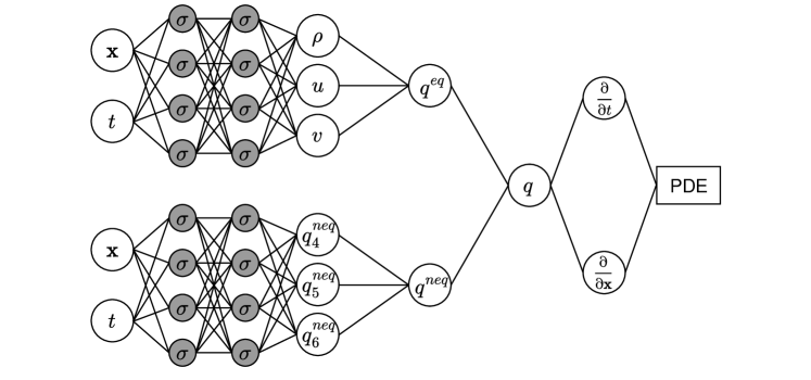
In this work, we train two separate networks for the equilibrium and non-equilibrium state variables similar to [24, 25, 26]. The network structure can be seen in Figure 1. Both networks take spatio-temporal coordinates as the input. The equilibrium network outputs the primitive flow variables, velocity, and density. Using these primitive flow variables, the equilibrium state variables can be calculated. The second network outputs the non-equilibrium state variables. The number of non-equilibrium state variables is three, as it can be seen in Equation (12) since . We also scale the output of the second network with the relaxation time parameter ; otherwise, the values are close to zero, and it does not converge to physically admittable results. The boundary conditions are employed by using the primitive flow variables in the first neural network with equilibrium state variables. The non-equilibrium network accepts boundary conditions using Equation (9).
We have also used Fourier feature embedding to enrich the input space [29, 20]. The input coordinates are mapped into a higher-dimensional feature space using random Fourier mapping as
| (19) |
where all the entries in is sampled from a Gaussian distribution with the standard deviation being a user-specified parameter.
3 Numerical Tests
In this section, the results of the Galerkin-Boltzmann formulation are presented. The PINN code is written with PyTorch as the backend. We select ADAM optimizer and hyperbolic tangent activation function for all the test cases presented. All the results shown here are obtained using a Dell Precision laptop with an Nvidia RTX A1000 laptop GPU.
3.1 Kovasznay Flow
We first test our formulation to simulate a two-dimensional steady Kovasznay flow [30]. The rectangular domain is between and . The exact solutions are given as
| (20a) | |||
| (20b) | |||
where and represents the fluid velocity and
| (21) |
We employ the test case from [24], where they have used a two-dimensional-nine-speed (D2Q9) model as a lattice-Boltzmann method. The flow variables are , , , , which makes . This enables us to stay in the weakly compressible regime. Using these values, we get the kinematic viscosity as and the relaxation parameter as . The boundary conditions are given using Equation (20) for the velocities. The density boundary condition is given as in all boundaries.
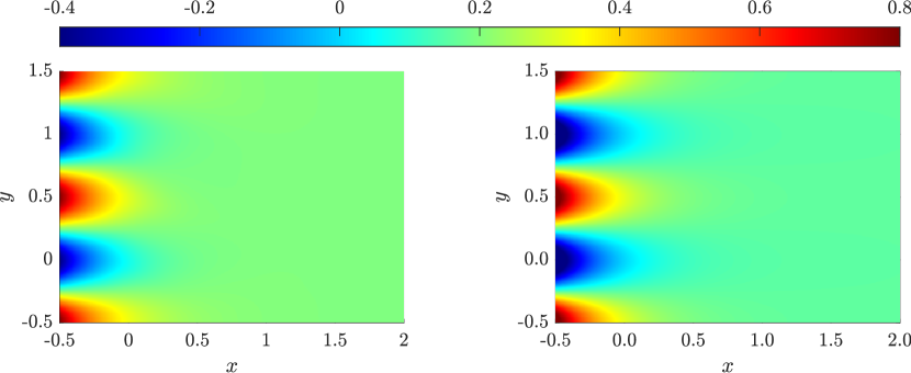
We have used 4 layers with 128 neurons in both equilibrium and non-equilibrium networks for the network architecture. Both networks are initialized with the Glorot scheme [31] and trained for 20000 epochs. The learning rate starts at 0.005 and exponentially decays with a decay rate of 0.99 for the ADAM optimizer. The PINN solution with the exact solutions for and velocities can be seen in Figure 2. We can accurately capture the flow field using PINN with the Galerkin-Boltzmann formulation compared to the exact solution.
We also solved the same problem using incompressible Navier-Stokes (INS) equations with PINN. The flow parameters are the same as the solution in the Galerkin-Boltzmann formulation. We employed only one network with the same number of layers and neurons (4 hidden layers with 128 neurons) to get the primitive flow variables of pressure and velocities with the Fourier feature embedding. The number of epochs for the training is again 20000.
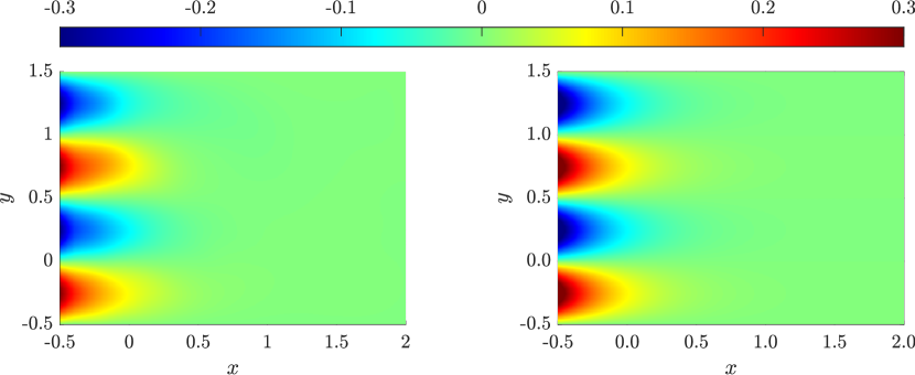
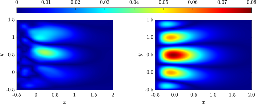
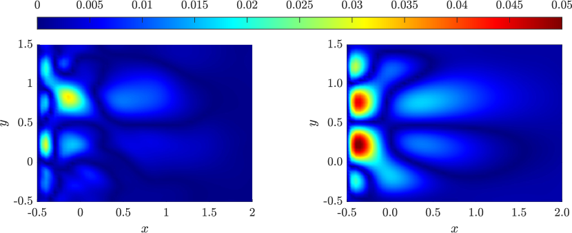
The error contours for the velocities for both Galerkin-Boltzmann and INS solutions are presented in Figure 3. As can be seen from the figure, PINN can predict a more accurate solution with the Galerkin-Boltzmann formulation under these training settings than INS. Especially INS formulation struggles more to capture the true solution near the boundaries without any special treatment. We have also presented the errors for and velocity solutions under both formulations in Table 1 with the total training time. Although the Galerkin-Boltzmann formulation uses two neural networks, hence it has more hyperparameters, the training time is comparable with the INS formulation. This can result from the special structure of the PDE system, which uses only first-order derivatives.
| Formulation | Training time (min) | |||||
|---|---|---|---|---|---|---|
| Galerkin-Boltzmann | 0.049 | 0.028 | 32.47 | |||
| INS | 0.096 | 0.044 | 30.30 |
3.2 Taylor-Green Vortex
We solve the Taylor-Green vortex problem, which has a time-dependent exact solution to test the formulation in unsteady problems. The computational domain is and . The exact solution is given as
| (22a) | |||
| (22b) | |||
where and are the and components of fluid velocity respectively.
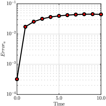
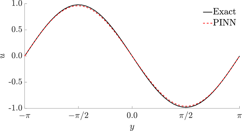
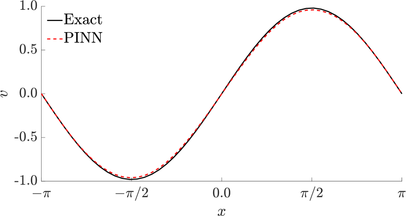
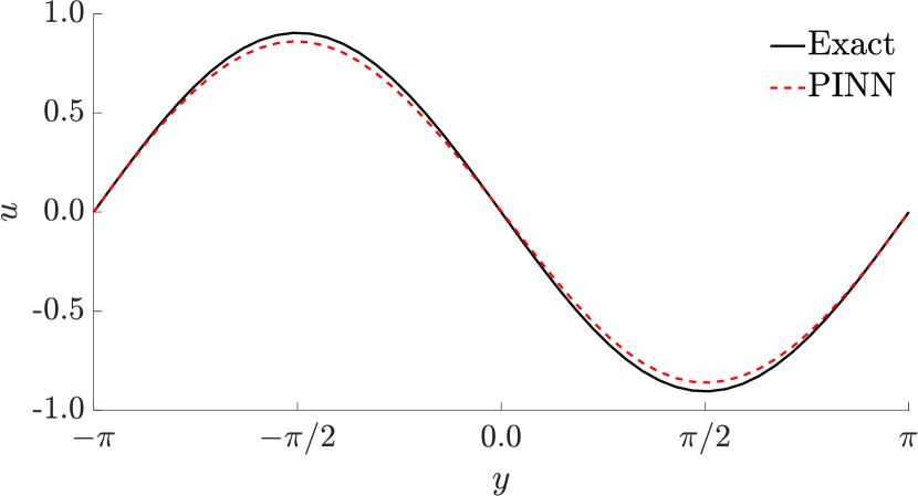
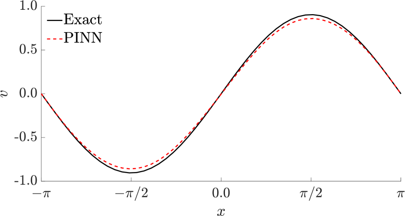
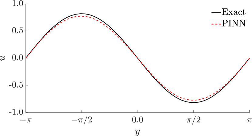
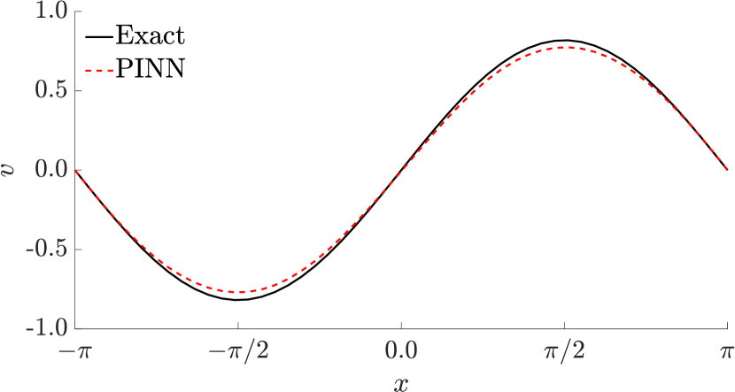
For the PINN solution, we again used two networks with 4 hidden layers and 128 neurons in each layer. We sampled 20000 points in the spatiotemporal domain and 1000 points in each boundary and initial time. We set and for the unsteady simulations in . We have used Equation (22) for the boundary and initial conditions of the velocities. We have initialized the field with . The initial learning rate is set to and exponentially decays with a decay rate of 0.99. Both networks are initialized with the Glorot scheme and trained for 50000 epochs. We have presented the evaluation of normalized errors of velocity in Figure 4 through the time domain. The error is smaller at times closer to the initial condition and increases as the information propagates in time [23]. We have also provided centerline velocity profiles compared with the exact solutions in Figure 5. This demonstrates the accuracy of PINN using Galerkin-Boltzmann equations in time-dependent problems.
3.3 Flow Over a Square Cylinder
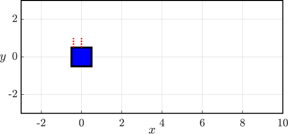
In our next test case, we study the flow over a square as a forward and inverse problem. The computational domain is bounded by and . The square center sits on (0,0) with a side length of 1. The uniform flow is from the inlet at with a magnitude of 1.0. The Reynolds number is , the speed of sound is , resulting in a Mach number of , and the relaxation time parameter . We analyze the solution by comparing the accuracy of the boundary layer velocity profiles at two different locations at and on the top surface of the square cylinder. The computational domain and the locations of the analyzed boundary layer velocity profiles can be seen in Figure 6.
3.3.1 Forward Solution
We have solved the uniform flow over a square cylinder test case using a limited number of data from a high-fidelity solver. We have used libParanumal [32] in which the Galerkin-Boltzmann formulation is implemented using the discontinuous Galerkin method for providing the labeled data. The high-fidelity simulation is conducted with a mesh with triangular elements and polynomial order . A perfectly matched layer is utilized to suppress the unphysical incoming waves from the boundary.
For the PINN solution, we used networks with 4 hidden layers with 128 neurons. We sampled 5000 collocation points, 500 points on each outer boundary, and 100 points on all sides of the square. We also fuse 150 random labeled data from libParanumal. The training is performed for 25000 epochs in 35.44 minutes.
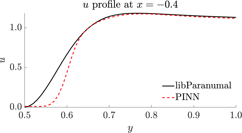
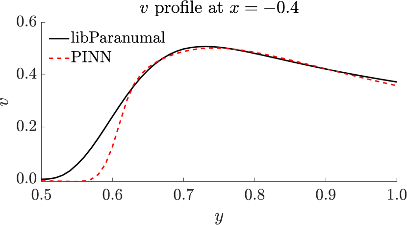
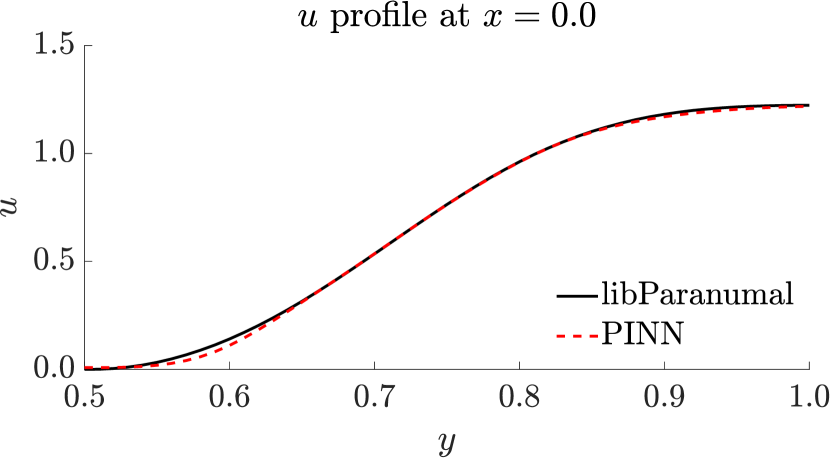
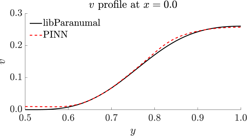
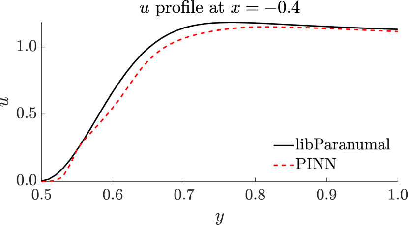
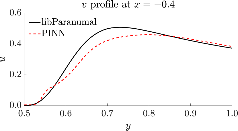
We compare and analyze the boundary layer profile at the top of the square using the high-fidelity data and PINN solution. In Figure 7, we present the and boundary velocity profiles between at and . The corner of the square is at , and therefore, the flow separates from the wall. The line at is a high-gradient region, and PINN struggles to find an accurate solution, especially near the boundary. However, the solution can follow a trend similar to the high-fidelity solution obtained by libParanumal. At the boundary, the flow variables are not exactly satisfied since we implemented soft boundary conditions. At , the middle point of the square, the gradient is lower than the corner of the square, and PINN can capture the velocity field accurately.
To enhance the performance of PINN to capture the boundary layer profile more precisely we have tried increasing the collocation point density around the square. We have created a zone in and and sampled 1000 points inside this zone, excluding the square boundary. We sampled 4000 points from the remaining domain, and the number of boundary samples is the same. The result is presented in Figure 8. It can be seen that we can achieve an accurate boundary layer profile compared to the uniform sampling through the whole domain, especially in the near region of the boundary.
3.3.2 Inverse Solution
For the same test case, we have also tested the performance of this formulation in an inverse problem. We focus on predicting the relaxation time parameter with the high-fidelity data from libParanumal. Since this parameter is a very low number, we scaled the trainable parameter by an order of . This way, the neural network predicts 10000 times . The order is rescaled to its original order of magnitude in the PDE. The neural networks are trained for 25000 epochs with an initial learning rate of with an exponential decay rate of 0.99. 5000 labeled data points are used with an additional 5000 collocation points to satisfy the PDE. We assign 10 times higher weight to the residual loss to increase the learning towards the PDE along with the data loss. The PINN predicts the parameter as , which is very close to the true value of parameter .
4 Conclusion
In this work, we presented the Galerkin-Boltzmann formulation in a PINN framework and used it to simulate flows in weakly compressible regimes. The Galerkin-Boltzmann formulation with the BGK collision model is discretized with second-order Hermite polynomials in velocity space, leading to a first-order system of equations. Reducing the order of the derivatives compared to the Navier-Stokes equations and the number of equations compared with the widely used D2Q9 lattice Boltzmann formulation makes this system well-suited for PINN architectures. We created two different neural networks to separate the training of equilibrium and non-equilibrium states to overcome the scale discrepancy between the advection and the collision terms. We solved the Kovasznay flow using the Galerkin-Boltzmann formulation and the incompressible Navier-Stokes equations in PINN. The Galerkin-Boltzmann formulation results in low errors in velocity predictions in a comparable training time. We also presented the accuracy of the solver in unsteady problems using the Taylor-Green vortex. We analyzed boundary layer profiles of flow over a square test case by providing limited data from a high-fidelity solver. PINN struggles to predict accurate boundary layer velocity profiles in the regions where the flow is separated. However, increasing the collocation point density can overcome this challenge and provide more accurate solutions. These numerical tests show promising results in predicting flows in weakly compressible regimes.
References
- [1] C. Chattopadhyay, U. Heinz, and T. Schaefer, “Fluid dynamics from the Boltzmann equation using a maximum entropy distribution,” 2023. arXiv:2307.10769.
- [2] C. Cercignani, “The Boltzmann Equation,” in The Boltzmann Equation and Its Applications, pp. 40–103, New York, NY: Springer, 1988.
- [3] P. L. Bhatnagar, E. P. Gross, and M. Krook, “A model for collision processes in gases. I. Small amplitude processes in charged and neutral one-component systems,” Physical Review, vol. 94, no. 3, pp. 511–525, 1954.
- [4] D. Yu, R. Mei, L.-S. Luo, and W. Shyy, “Viscous flow computations with the method of lattice Boltzmann equation,” Progress in Aerospace Sciences, vol. 39, no. 5, pp. 329–367, 2003.
- [5] P. Lallemand, L.-S. Luo, M. Krafczyk, and W.-A. Yong, “The lattice Boltzmann method for nearly incompressible flows,” Journal of Computational Physics, vol. 431, p. 109713, 2021.
- [6] G. Wissocq and P. Sagaut, “Hydrodynamic limits and numerical errors of isothermal lattice Boltzmann schemes,” Journal of Computational Physics, vol. 450, p. 110858, 2022.
- [7] C. K. Aidun and J. R. Clausen, “Lattice-Boltzmann method for complex flows,” Annual Review of Fluid Mechanics, vol. 42, pp. 439–472, 2010.
- [8] M. Min and T. Lee, “A spectral-element discontinuous Galerkin lattice Boltzmann method for nearly incompressible flows,” Journal of Computational Physics, vol. 230, no. 1, pp. 245–259, 2011.
- [9] W. Li, “High order spectral difference lattice Boltzmann method for incompressible hydrodynamics,” Journal of Computational Physics, vol. 345, pp. 618–636, 2017.
- [10] A. Karakus, N. Chalmers, J. S. Hesthaven, and T. Warburton, “Discontinuous Galerkin discretizations of the Boltzmann–BGK equations for nearly incompressible flows: Semi-analytic time stepping and absorbing boundary layers,” Journal of Computational Physics, vol. 390, pp. 175–202, 2019.
- [11] H. Lee and I. S. Kang, “Neural algorithm for solving differential equations,” Journal of Computational Physics, vol. 91, no. 1, pp. 110–131, 1990.
- [12] I. E. Lagaris, A. Likas, and D. I. Fotiadis, “Artificial neural networks for solving ordinary and partial differential equations,” IEEE transactions on neural networks, vol. 9, no. 5, pp. 987–1000, 1998.
- [13] J. Sirignano and K. Spiliopoulos, “DGM: A deep learning algorithm for solving partial differential equations,” Journal of Computational Physics, vol. 375, pp. 1339–1364, 2018.
- [14] M. Raissi, P. Perdikaris, and G. Karniadakis, “Physics-informed neural networks: A deep learning framework for solving forward and inverse problems involving nonlinear partial differential equations,” Journal of Computational Physics, vol. 378, pp. 686–707, 2019.
- [15] A. G. Baydin, B. A. Pearlmutter, A. A. Radul, and J. M. Siskind, “Automatic differentiation in machine learning: a survey,” The Journal of Machine Learning Research, vol. 18, no. 1, pp. 5595–5637, 2017.
- [16] G. E. Karniadakis, I. G. Kevrekidis, L. Lu, P. Perdikaris, S. Wang, and L. Yang, “Physics-informed machine learning,” Nature Reviews Physics, 2021.
- [17] S. Wang, X. Yu, and P. Perdikaris, “When and why PINNs fail to train: A neural tangent kernel perspective,” Journal of Computational Physics, vol. 449, p. 110768, 2022.
- [18] A. Jacot, F. Gabriel, and C. Hongler, “Neural Tangent Kernel: Convergence and generalization in neural networks,” in Advances in Neural Information Processing Systems, vol. 31, Curran Associates, Inc., 2018.
- [19] S. Wang, Y. Teng, and P. Perdikaris, “Understanding and Mitigating Gradient Flow Pathologies in Physics-Informed Neural Networks,” SIAM Journal on Scientific Computing, vol. 43, no. 5, pp. A3055–A3081, 2021.
- [20] S. Wang, H. Wang, and P. Perdikaris, “On the eigenvector bias of Fourier feature networks: From regression to solving multi-scale PDEs with physics-informed neural networks,” Computer Methods in Applied Mechanics and Engineering, vol. 384, p. 113938, 2021.
- [21] L. D. McClenny and U. M. Braga-Neto, “Self-adaptive physics-informed neural networks,” Journal of Computational Physics, vol. 474, p. 111722, 2023.
- [22] S. J. Anagnostopoulos, J. D. Toscano, N. Stergiopulos, and G. E. Karniadakis, “Residual-based attention in physics-informed neural networks,” Computer Methods in Applied Mechanics and Engineering, vol. 421, p. 116805, 2024.
- [23] S. Wang, S. Sankaran, and P. Perdikaris, “Respecting causality for training physics-informed neural networks,” Computer Methods in Applied Mechanics and Engineering, vol. 421, p. 116813, 2024.
- [24] Q. Lou, X. Meng, and G. E. Karniadakis, “Physics-informed neural networks for solving forward and inverse flow problems via the Boltzmann-BGK formulation,” Journal of Computational Physics, vol. 447, p. 110676, 2021.
- [25] R. Li, E. Lee, and T. Luo, “Physics-informed neural networks for solving multiscale mode-resolved phonon Boltzmann transport equation,” Materials Today Physics, vol. 19, p. 100429, 2021.
- [26] J. Zhou, R. Li, and T. Luo, “Physics-informed neural networks for solving time-dependent mode-resolved phonon Boltzmann transport equation,” npj Computational Materials, vol. 9, no. 1, pp. 1–9, 2023.
- [27] J. Oh, S. Y. Cho, S.-B. Yun, E. Park, and Y. Hong, “Separable Physics-informed Neural Networks for Solving the BGK Model of the Boltzmann Equation,” Mar. 2024. arXiv:2403.06342.
- [28] J. Tölke, M. Krafczyk, M. Schulz, and E. Rank, “Discretization of the Boltzmann equation in velocity space using a Galerkin approach,” Computer Physics Communications, vol. 129, no. 1, pp. 91–99, 2000.
- [29] M. Tancik, P. P. Srinivasan, B. Mildenhall, S. Fridovich-Keil, N. Raghavan, U. Singhal, R. Ramamoorthi, J. T. Barron, and R. Ng, “Fourier features let networks learn high frequency functions in low dimensional domains,” 2020. arXiv: 2006.10739.
- [30] L. I. G. Kovasznay, “Laminar flow behind a two-dimensional grid,” in Mathematical Proceedings of the Cambridge Philosophical Society, vol. 44, pp. 58–62, Cambridge University Press, 1948.
- [31] X. Glorot and Y. Bengio, “Understanding the difficulty of training deep feedforward neural networks,” in Proceedings of the Thirteenth International Conference on Artificial Intelligence and Statistics, pp. 249–256, JMLR Workshop and Conference Proceedings, 2010.
- [32] N. Chalmers, A. Karakus, A. P. Austin, K. Swirydowicz, and T. Warburton, “libParanumal: a performance portable high-order finite element library,” 2022. Release 0.5.0.