Quantum Wasserstein Compilation:
Unitary Compilation using the Quantum Earth Mover’s Distance

Abstract

Despite advances in the development of quantum computers, the practical application of quantum algorithms remains outside the current range of so-called noisy intermediate-scale quantum devices. Now and beyond, quantum circuit compilation (QCC) is a crucial component of any quantum algorithm execution. Besides translating a circuit into hardware-specific gates, it can optimize circuit depth and adapt to noise. Variational quantum circuit compilation (VQCC) optimizes the parameters of an ansatz according to the goal to reproduce a given unitary transformation. In this work, we present a VQCC-objective function called the quantum Wasserstein compilation (QWC) cost function that is based on the quantum Wasserstein distance of order 1. We show that the QWC cost function upper bounds the average infidelity of two circuits. An estimation method based on measurements of local Pauli-observable is utilized in a generative adversarial network to learn a given quantum circuit. We demonstrate the efficacy of QWC cost function by compiling a single layer hardware efficient ansatz (HEA) as both the target and the ansatz, and comparing other cost functions such as the Loschmidt echo test (LET) and the Hilbert-Schmidt test (HST). Finally, our experiments also demonstrate that QWC as a cost function can mitigate the barren plateaus for the particular problem we consider.

I Introduction

The compilation of quantum circuits is as crucial to quantum computing as the compilation of human-readable code into executable machine language is to traditional computing. By compilation, we are able to focus on the fundamental operations in both quantum and traditional computing thanks to the abstraction of the underlying complexity.

Quantum circuit compilation (QCC) entails translating a target quantum algorithm into an executable quantum circuit compatible with real quantum computing hardware. This intricate process must account for the target hardware constraints, including the available gate alphabet, qubit connection graph, and depth restrictions. Additionally, a strategic approach may consider individual error rates of single and two-qubit operations, single-qubit decoherence rates, and readout errors during the rewriting process to minimize the probability of error-prone execution. In the context of noisy intermediate-scale quantum (NISQ) computing, these optimizations are not mere conveniences but pivotal elements[1]. The considerations in the QCC process thus underscore its critical importance in the era of NISQ computing.

One QCC technique relies on the variational quantum computing paradigm, i.e. the optimization of parameters of a circuit towards an objective function. The evaluation of the cost function for this optimization, is carried out directly on the quantum computer [2] unlike other cost functions which are evaluated classically and thus scale exponentially with the number of qubits. Recent findings indicate that current methods of variational quantum circuit compilation (VQCC) do not fully exploit the potential of the data that is made available to them, because their data requirements grow exponentially with the size of the target system [3, 4]. Although, based on the findings of Caro et al. [5], a polynomial amount of training data should be sufficient to approximately compile a target circuit. This encourages us to look for improved methods of VQCC.

Until now, methods of variational compilation have been closely related to the state overlap of quantum states. However, the state overlap has two fundamental properties that render it ineffective as a cost function: Firstly, parts of the systems can completely dominate the state overlap. If the state of a subsystem is orthogonal to the state of its variational counterpart, the overlap between the entire system states is zero, as is the overlap between the subsystem states. Secondly, the state overlap for two randomly picked quantum states decreases exponentially with system size. The vanishing of the state overlap also results in a learning signal that is exponentially smaller and hence exponentially more expensive to measure when we use the state overlap as an objective function.

Therefore, we propose introducing a cost function for VQCC based on a fundamentally different metric: the quantum Wasserstein distance of order 1. This distance, also known as the quantum $W_{1}$ distance or the quantum Earth Mover’s (EM) distance, offers an alternative approach to measuring differences between quantum states. Unlike the trace distance or quantum fidelity, the quantum EM distance is not unitarily invariant. Additionally, it is additive rather than multiplicative with respect to subsystems, preventing any one subsystem from dominating the distance. Consequently, the quantum $W_{1}$ distance grows linearly with the size of the quantum system [6]. These very promising properties motivate us to formulate a compilation method based on this distance.

The paper is organized as follows: Section II introduces the preliminaries of unitary compilation along with the various cost functions which are used in literature. Section III reviews previous work on variational compilation with and without quantum machine learning method. Section IV discusses the concepts which are important in our approach. Section V details the experimental setup and discusses the results. Section VI concludes the paper with some discussion of our approach. The Appendix provides a brief overview of the theoretical background and the various cost functions used in this work.

II Preliminaries

II.1 Unitary Compilation

In this section, we will review unitary compilation in the variational quantum machine learning framework [7]. Here, compilation describes the process of finding a decomposition of a unitary transformation $V$ into a specific set of parameterized unitaries available on the hardware $\{U_{i}(\theta_{i})\}$, i.e.

$$V\approx U_{1}(\theta_{1})U_{2}(\theta_{2})U_{3}(\theta_{3})\dots$$ (1)

with possibly independent parameters $\theta_{i}$. The unitary compilation process is thereby twofold: a) chose an appropriate ansatz represented by the kind of parameterized unitaries $U_{i}$ and b) find the optimal parameters (see Fig. 1).

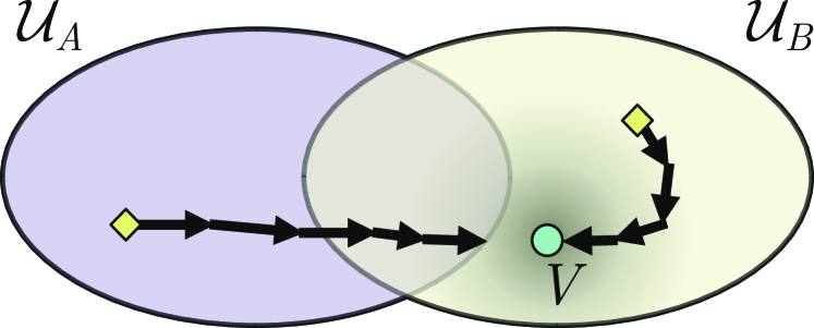
Figure 1: The two manifolds $\mathcal{U}_{A}$ and $\mathcal{U}_{B}$ represent two families of unitaries created by different ansätze. $\diamond$ denote the starting point of the optimization of the continuous parameters, respectively. Here, the ansatz $B$ can reach the optimal unitary $V$. In contrast, ansatz $A$ only admits an (possibly bad) approximation. Note: the optimization landscape is non-convex.

Determining an appropriate ansatz ad-hoc poses a complex problem, primarily due to the intrinsic trade-off between its expressivity and trainability. Higher expressivity is linked to vanishing gradients [8]. Therefore, the selection of an ansatz demands use of intuition and application of prior knowledge about the target unitary. Underlying symmetries and patterns might be used to train an ansatz that is not excessively expressive [9].

Addressing the issue of expressivity versus trainability necessitates exploring strategies to update the structure. One possible approach includes incrementally adding layers to the ansatz until a satisfactory approximation of the target unitary is achieved [2]. This method offers the advantage of progressively enhancing the ansatz’s expressivity. During the extension, the complexity increase can be limited by only accepting updates that improve the approximation quality.

Another approach to bolstering the expressivity of an ansatz, while maintaining control over its complexity, involves a technique called variable ansatz [10]. This optimization technique adds and removes gate sequences during the continuous parameter optimization. This enables searching for appropriate solutions while keeping the candidates shallow and thereby potentially trainable for local cost functions [11].

The technique that we developed in this work tackles the problem of finding optimal parameters for a given ansatz. In other words, we train a parameterized quantum circuit, represented by the unitary operator $U(\bm{\theta})$, such that it is close to a given target unitary operator $V$. Since closeness for unitary transformations can be defined in several ways, it makes sense to have various distance measures for various applications.

The applications of unitary compilation can be classified into three categories: (a) full unitary matrix compilation (FUMC), (b) fixed input states compilation (FISC) (for example, as used in quantum data encoding schemes) and (c) single input state compilation (SISC) (for examples, used in state preparation circuits in quantum chemistry). In FUMC, we are aiming to reproduce the complete unitary matrix and hence mimic the target evolution of every possible input state. In consequence, the average fidelity is the natural figure of merit for FUMC.

Definition 1 (Average Fidelity [12, 2]).

Given two unitary transformations $U$ and $V$, the average fidelity between them is defined as:

$$\overline{F}(U,V)=\int\dl\psi\lvert\braket{\psi}{V^{\dagger}U}{\psi}\rvert^{2}.$$ (2)

Here, $\dl\psi$ represents the integration over the unitarily invariant Fubini-Study measure on pure states.

This measure quantifies how closely the two transformations resemble each other for arbitrary input states. Alternatively in FISC, when we are only interested in reproducing the evolution of a fixed state set $\mathcal{A}$ under the target unitary $V$, a much weaker figure of merit is sufficient, namely the set-average state fidelity:

$$F(U,V,\mathcal{A})=\frac{1}{|\mathcal{A}|}\sum_{\ket{\psi}\in\mathcal{A}}\lvert\braket{\psi}{V^{\dagger}U}{\psi}\rvert^{2}$$ (3)

with $|\mathcal{A}|$ being the number of states in $\mathcal{A}$. In SISC, the cardinality of $\mathcal{A}$ is one.

II.2 Cost Functions of Variational Compilation

The transformation of a parameterized unitary operator $U(\bm{\theta})$ such that it closely mimics the given target unitary operator $V$ is an optimization procedure which requires defining a cost function which can be used as the single metric for minimization/maximization. For variational compilation we focus on two such metrics. The Hilbert-Schmidt test was introduced by Khatri et al. [2] for variational compilation and can be measured using a Bell state and a Bell measurement directly on a quantum computer, if both unitaries are coherently accessible (i.e. on the same quantum hardware or in an entangled system). It is defined in terms of the target unitary $V$, the ansatz $U$ and the number of qubits $n$ as

$$C_{\text{HST}}=1-|\text{Tr}(V^{\dagger}U)|^{2}/4^{n}$$ (4)

Notice how, this metric does not depend on the input states used. Minimization of the cost function ensures closeness between the unitary $U$ and $V$. This metric is related to the average fidelity defined in Eq. (2) by the relation

$$\bar{F}(U,V)=\frac{2^{n}+|\text{Tr}(V^{\dagger}U)|^{2}}{4^{n}+2^{n}}$$ (5)

The second metric which will also be useful is the Loschmidt echo test. The Loschmidt echo was introduced in [13] and further used for FISC in [14] as the Loschmidt echo test (LET). It is defined as the overlap of an initial state $|\psi_{0}\rangle$ and the evolution of the same state under the unitary $V^{\dagger}U$. Thus for a fixed input state $|\psi_{0}\rangle$ the cost function is defined as the LET metric is defined as $|\langle\psi_{0}|V^{\dagger}U|\psi_{0}\rangle|^{2}$. Since our focus is on FUMC the LET needs to be generalised to account for multiple random input states. We thus define

$$C_{\text{LET}}=1-\frac{1}{|\mathcal{A}|}\sum_{\psi\in\mathcal{A}}|\langle\psi|V^{\dagger}U|\psi\rangle|^{2}$$ (6)

Both HST and LET as described above require measuring all the $n$ qubits and the cost functions suffer from a vanishing gradient problem if evaluated on a quantum computer. To address this, local HST (LHST) and local LET (LLET) were introduced. The detailed circuit implementation of both HST, LET and their local counterparts are given in Ref [14] A detailed discussion of other metrics used in quantum information theory is available in [15].

II.3 The Quantum Wasserstein Distance of Order 1

De Palma et al. [16] introduce the Wasserstein distance of order 1 for quantum states (or quantum $W_{1}$ distance). It is a generalization of the classical Wasserstein distance for probability distributions (also called earth mover’s distance) to quantum states. It has an interpretation as a continuous version of a quantum Hamming distance which could be intuitively described as the number of differing qubits. The formulation given in the work is not directly useful, but instead the dual formulation enables the practical use of the quantum $W_{1}$ distance which is defined in terms of the quantum Lipschitz constant [16].

Proposition 1.

For two $n$-qubit quantum states $\rho,\sigma\in\mathcal{D}(\mathcal{H}_{n})$ (set of density operators), the quantum $W_{1}$ distance admits a dual formulation,

$$W_{1}(\rho,\sigma)=\lVert\rho-\sigma\rVert_{W_{1}}:=\max(\mathrm{Tr}[H(\rho-\sigma)]:\\ H\in\mathcal{O}(\mathcal{H}_{n}),||H||_{L}\leq 1)$$ (7)

with $\mathcal{O}(\mathcal{H}_{n})$ being the set of observables in $\mathcal{H}_{n}$ and $||\cdot||_{L}$ the quantum Lipschitz constant as defined in De Palma et al. [16].

In the context of VQCC, the quantum $W_{1}$ distance has several intriguing properties, the most important of which is that it is not unitarily invariant. While this does not seem like an advantage, it makes the quantum $W_{1}$ fundamentally different from better known distance measures of quantum states like the trace distance or the quantum fidelity. As Kiani et al. [6] pointed out, this property facilitates the learning of quantum states: consider we want to learn and reproduce a state $\ket{\text{GHZ}_{2}}\ket{1}$ and our initial state is $\ket{000}$. If we change the state during the learning from the initial state to $\ket{\text{GHZ}_{2}}\ket{0}$ then this significant improvement towards the target should be admitted by the cost function. No unitarily invariant distance can discriminate between the three pair-wise orthogonal states and hence indicate the improvement. As shown in [17], the quantum EM distance is super-additive with respect to the tensor product, i.e. $W_{1}(\rho,\sigma)\geq W_{1}(\rho_{1..k},\sigma_{1...k})+W_{1}(\rho_{k+1..n},\sigma_{k+1...n})$ for two quantum states $\rho,\sigma$ of $n$-qubits and any $k=1,...,n-1$. $\rho_{1..k}$ and $\rho_{k+1...n}$ are the marginal states over the first $k$ and last $n-k$ qubits respectively. This ensures good linear scaling of the distance measure with the number of qubits and consequently for the gradient calculations.

To justify the usage of the quantum $W_{1}$ distance in VQCC, we examine the containment given by the trace norm $\lVert\cdot\rVert_{1}$ [16],

$$\frac{1}{2}\lVert\rho-\sigma\rVert_{1}\leq\lVert\rho-\sigma\rVert_{W_{1}}\leq\frac{n}{2}\lVert\rho-\sigma\rVert_{1}$$ (8)

where

$$\rho,\sigma\in\mathcal{D}(\mathcal{H}_{n})$$

From there, we can derive (see Appendix A) an upper bound for the infidelity for small quantum $W_{1}$ distances of mixed states, i.e. $0\leq\lVert\rho-\sigma\rVert_{W_{1}}\leq 1$,

$$2\lVert\rho-\sigma\rVert_{W_{1}}\geq 1-F(\rho,\sigma).$$ (9)

Additionally, we find for pure states a stronger upper bound for the infidelity holds for arbitrary $W_{1}$ distances,

$$\big{\lVert}\ket{\psi}\bra{\psi}-\ket{\phi}\bra{\phi}\big{\lVert}_{W_{1}}^{2}\geq 1-F(\ket{\psi},\ket{\phi}).$$ (10)

This upper bound for the infidelity of pure states in terms of the quantum $W_{1}$ norm will motivate our definition of the Wasserstein compilation cost.

III Related Work

Using quantum computers for quantum compiling in the form of variational circuits was introduced by Khatri et al. [2] with the cost function Eq. (4). Successful training of HST and LHST was demonstrated for unitaries with up to 9 qubits, with and without noisy simulations. On the other hand, the authors demonstrated the presence of barren plateaus in the gradients of the cost function with just depth-one circuits. The problem of barren plateaus in variational quantum circuits has been shown to have an exponential decay of variance of the gradients as the number of qubit grows [18]. So, significant research has focused on addressing the problem of barren plateaus in variational quantum circuits. First work in this direction was done in [19], where the technique involved randomly selecting some of the initial parameter values and then choosing the remaining values so that the circuit is a sequence of shallow blocks that each evaluates to the identity. The scaling of variance of the gradient of the energy expectation with respect to the number of qubits stayed constant when the state was initialized to be an equal superposition of all states.

Since in this work, we make use of a learning algorithm, we point out previous work done to address the question of amount of training data required for successful learning and generalization. The work by Caro et al. [5] establishes theoretical bounds on the generalization error in variational quantum machine learning. The generalization error is approximately upper bounded by $\sqrt{T/N}$ where $T$ is the number of parametrized gates, and $N$ is the training data size. The generalization error is the difference between the prediction and training errors, which we want to minimize.

IV Our Work

In this section, we introduce quantum Wasserstein compilation (QWC) as an extension of the quantum EM distance for comparing unitaries. It is based on the idea of simultaneously reducing the estimated quantum EM distance of output states for multiple different input states. In Section IV.1, we derive an ideal cost function that is based on this idea and indicate its significance for circuit compiling. Then, in Section IV.2 we will formulate an approximation of the cost function that is directly accessible by executing Pauli measurements. In Section IV.3, we will briefly describe the state ensemble needed as input to the unitaries during compilation. Finally in Section IV.4, we will describe the learning algorithm.

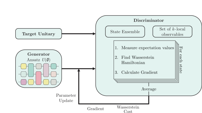
Figure 2: Overview of the compiling algorithm. The target unitary and the parameterized circuit acting as the generator are assessed by the discriminator which calculates the Wasserstein compilation cost. The distance estimation requires a state ensemble acting as input states for target and generator and a set of $k$-local observables whose expectation values are measured. A Wasserstein Hamiltonian can be constructed from the differences of the expectation values and the gradient of the averaged cost can be used for a updating the parameters of the generator.

IV.1 Ideal Cost

As outlined in Section II.3, the quantum $W_{1}$ distance is a measure for the closeness of two quantum states. We will now extend this distance to measuring the closeness of two unitary operators, $U$ and $V$, by applying the operators on (pure) quantum states and measuring the pairwise distances:

Definition 2 (Quantum Wasserstein Compilation Cost).

Let $U,V$ be unitary operators on $\mathcal{H}$ and $\ket{\psi}$ be a quantum state in $\mathcal{H}$. Then the quantum Wasserstein compilation distance is defined as

$$C_{QW}(U,V)=\int_{\psi}\dl{\psi}\>W_{1}^{2}\Big{(}U\ket{\psi},V\ket{\psi}\Big{)}$$ (11)

where $\dl\psi$ is the Fubini-Study metric.

We chose to define the QWC cost in Eq. (11) as the squared $W_{1}$ distance since it then acts directly as an upper bound for the average infidelity as shown below:

Proposition 2.

Let $U,V$ be unitary operators on $\mathcal{H}$. Then the following inequality holds between the QWC cost $C_{QW}(U,V)$ and the average fidelity $\overline{F}(U,V)$

$$C_{QW}(U,V)\geq 1-\overline{F}(U,V).$$ (12)

Proof.

We use that the quantum $W_{1}$ norm is an upper bound for the infidelity that we derive in the Appendix A, Eq. (10). Starting from the definition of the QWC cost in Eq. (11), we can directly upper bound the average fidelity:

$$C_{QW}(U,V) =\int_{\psi}\dl{\psi}\>W_{1}^{2}\Big{(}U\ket{\psi},V\ket{\psi}\Big{)}$$ (13)

$$\geq\int_{\psi}\dl{\psi}\>\left(1-F(U\ket{\psi},V\ket{\psi})\right)$$ (14)

$$=1-\overline{F}(U,V).$$ (15)

∎

Proposition 2 sheds light on the operational meaning of $C_{\text{QW}}$ in quantum circuit compilation. It can be used as a cost function in training a parameterized quantum circuit $U(\theta)$ to mimic the action of a target circuit $V$ accordingly to the quantum-assisted quantum compilation scheme described in Khatri et al. [2].

IV.2 Empirical Cost

In order to calculate the cost in Eq. (11) we need to first estimate the quantum EM distance as defined in Eq. (7). For this, we begin by choosing the observables satisfying the quantum Lipschitz condition. We use the ansatz for $H$ that is a weighted sum of locally acting Pauli observables.

$$H=\sum_{m}w_{m}H_{m}\quad H_{m}=\bigotimes_{j=1}^{n}\sigma_{P_{j}}^{(j)}\quad P_{j}\in\{I,X,Y,Z\}$$ (16)

This ansatz has $4^{n}$ observables, which grows exponentially with the number of qubits. Inspired from Kiani et al. [6] we can restrict the set of observable $\mathcal{O}(\mathcal{H}_{n})$ to $\mathcal{O}(\mathcal{H}_{n})^{(k)}$. We define this as the set of Pauli strings that act non-trivially only on a subset of $k$-qubits, and refer to them as $k$-local Pauli observables. Using local Pauli operators restricts the growth of the number of Pauli observable to $\mathcal{O}(n^{k})$ for $k\ll n$. Thus we instead have the approximation

$$W_{1}^{(k)}=\max(\text{Tr}[H(\rho-\sigma)]:H\in\mathcal{O}(\mathcal{H}_{n})^{(k)},||H||_{L}<1)$$ (17)

Moreover, the space of all quantum states is growing exponentially fast in system size and even for small qubit numbers, is inaccessibly huge. To overcome this hurdle, we use a state ensemble $\mathcal{A}=\{|\psi\rangle_{s}\}$, restrict to $k$-local observables and measure the empirical distance:

$$\tilde{C}_{QW}^{(k)}(U,V,\mathcal{A})=\frac{1}{|\mathcal{A}|}\sum_{\psi\in\mathcal{A}}\left(W_{1}^{(k)}(U\ket{\psi},V\ket{\psi})\right)^{2}$$ (18)

The choice and size of the set of probe states $\mathcal{A}$ are decisive for the practical use of $\tilde{C}_{QW}^{(k)}$ as an optimization objective in VQCC. In the limit of infinitely many states that are sampled according to the Fubini-Study metric and no restriction on the locality of Pauli operators, the empirical quantum Wasserstein compilation distance becomes equivalent to the ideal distance from Eq. (11). The derivatives of the cost function with respect to a parameter $\theta\in\bm{\theta}$ can be directly calculated from the respective derivative of the EM distance[6], i.e. around a value $t$:

$$\diffp*{\tilde{C}_{QW}^{(k)}{U(\theta),V,\mathcal{A}}}{\theta}[\theta=t]=\frac{1}{|\mathcal{A}|}\sum_{\ket{\psi_{a}}\in\mathcal{A}}2W_{1}^{(k)}\Bigl{(}U(t)\ket{\psi_{a}},V\ket{\psi_{a}}\Bigr{)}\cdot\diffp*{W_{1}^{(k)}\Bigl{(}U(\theta)\ket{\psi_{a}},V\ket{\psi_{a}}\Bigr{)}}{\theta}[\theta=t]$$ (19)

Proposition 3.

Let $\rho(\bm{\theta})\in\mathcal{H}$ be a paramatrized quantum state and $\sigma\in\mathcal{H}$ a second quantum state. Furthermore, let $H_{W}(\bm{w})$ be the optimal $W_{1}$ observable that maximizes $W_{1}^{(k)}$. For a single parameter $\theta_{i}\in\bm{\theta}$ at $t$,

$$\frac{d}{d\theta_{i}}W_{1}^{(k)}(\rho(\bm{\theta}),\sigma)\Big{|}_{t}=\frac{d}{d\theta_{i}}\text{Tr}[\rho(\bm{\theta})H_{W}(\bm{w})]\Big{|}_{t}$$ (20)

The derivative $\diffp*{W_{1}^{(k)}\Bigl{(}U(\theta)\ket{\psi},V\ket{\psi}\Bigr{)}}{\theta}[\theta=t]$ can be evaluated using standard techniques like the parameter-shift rule [20].

Since we now have the cost function and its gradients, the only missing building block for learning unitaries is the choice of the state ensemble.

IV.3 State Ensembles

Our method for full unitary matrix compilation is dependent on a state ensemble $\mathcal{A}$. Caro et al. [21] showed that learning over a locally scrambled ensemble is equivalent to learning over the uniform distribution of states over the complete Hilbert space. This seminal result paves the way to use an ensemble of product states $\mathcal{S}_{\text{Haar}^{\otimes n}_{1}}$ where each product state is the combination of Haar-random single-qubit states. Random product states can be prepared using a shallow circuit of depth three in contrast to multi-qubit Haar-random states which require deep circuits.

While the sizes are determined for SISC and FISC, the number of states used to determine the empirical cost function is an important hyperparameter of FUMC. QWC for FUMC can use a fixed set $\mathcal{A}$ of input states which we will call fixed mode. Alternatively, the QWC can sample input states in each compilation step

It is an open question how much data in the form of quantum states and their output states are needed to successfully learn a given unitary. Some authors expect that compilation from data requires very large datasets [22, 23]. Recent results by Caro et al. [5] show that already training data suffice that has size polynomial in the number of qubits. The argument is based on the proposition that the required size of training data is roughly linear in the number of parameterized gates. As a matter of fact, virtually all the ansätze used in practice have significantly fewer parameters than the degrees of freedom of a corresponding unitary. Furthermore, the parameters are often not independent, leading to a further reduction of the actual number of degrees of freedom.

In this work, we will utilize another approximation: a SU(2) transformation $U_{3}(\theta,\phi,\lambda)$, parameterized by 3 angles, is applied to each qubit. Sampling each parameter randomly and uniformly between $(-\pi,\pi]$ creates a random product state. It is well known, that such a transformation $U_{3}$ can be decomposed into three rotational gates, for example using Z- and Y-rotations:

$$U_{3}(\theta,\phi,\lambda)=R_{\text{Z}}(\lambda)R_{\text{Y}}(\phi)R_{\text{Z}}(\theta).$$ (21)

Using a fixed set of states might decrease the number of circuit evaluations since the Pauli measurements for the probe states under the target evolution can be done in advance . On the other hand, using a set of states in the sampling mode increases computation, but allows for greater variability in the training process. We discuss our choice in the Experiments section.

IV.4 Learning a Unitary using QWC

In the previous sections, we introduced the empirical quantum Wasserstein compilation cost and its derivatives for parameterized unitaries (see Eq. (18)-(20)). Based on these ideas, we can formulate a procedure to learn a target unitary $V$, see Fig. 2.

The compilation is in the form of a quantum Wasserstein Generative Adversarial Net (qWGAN) inspired from Kiani et al. [6]. Quantum GAN is a quantum adversarial game [24], where the Nash equilibrium can be reached in an all-quantum game if the generator is expressive enough to reproduce the target and the discriminator has the capabilities to find a measurement that discriminates them. The expressivity of a quantum circuit specifies the set of unitary transformations it can reproduce and, of course, for a successful approximate compilation, there should be an approximation of the target unitary in this set. Due to the limited scope of this study, the expressivity of the generator was not explicitly addressed and assumed to be given. The discrimination ability, on the other hand, depends on several factors that were examined in this work. The generator is a variational quantum circuit with parameters $\bm{\theta}$ outputting a state $G(\bm{\theta})$, and the discriminator is the weighted Hamiltonian from Eq. (16) with $k$-local Pauli strings.

The first step of every optimization is measuring the expectation values of the Pauli observables $H_{m}\in\mathcal{O}^{(k)}_{n}$ for every input state $\ket{\psi_{a}}\in\mathcal{A}$ after evolving with the generator ansatz $\{G(\bm{\theta})\ket{\psi_{a}}\}$ ($\rho(\bm{\theta})$) and the target $\{V\ket{\psi_{a}}\}$ ($\sigma$). The expectation value difference is given by $c_{m}=\text{Tr}(\rho(\bm{\theta})H_{m})-\text{Tr}(\sigma H_{m})$. If the states and the observables are fixed, the result of the target can be cached and does not need to be measured again. Then we solve the linear program for the weights $w_{m}$

$$\begin{array}[]{ll@{}ll}\text{maximize}&\sum_{m}w_{m}c_{m}&\\ \text{constraint}&\sum_{m:i\in\mathcal{I}_{m}}|w_{m}|\leq 1/2\quad\forall i\in[n]\end{array}$$ (22)

Note, that the weights $w_{i}^{(a)}$ are sparse with only $n$ non-zero entries and the corresponding Pauli operators are called active.

The state-wise quantum $W_{1}$ distances $W_{1}^{(k)}$ can be measured from Eq. (17) with the Hamiltonian $H_{W}=\sum_{m\in\mathcal{M}}w_{m}^{*}H_{m}$ where $\mathcal{M}$ is the set of active Pauli operators and $w_{m}^{*}$ are the solutions to the linear program. Finally, the gradients of the state-wise distances can be derived (see Eq. (19)). These gradients are then averaged and used to perform a gradient-based update of the generator $G(\bm{\theta})$. In our experimental setup, the primary goal is to showcase the viability of our chosen approach. We specifically selected the hardware-efficient ansatz (HEA) as our target and ansatz for demonstration. The circuit diagram for HEA can be found in Fig. 3. We fix the parameters of the target and randomly choose a different set of parameters for the ansatz. This ensures that at least one solution exists for the compilation problem. Additionally, we compare two distinct entanglement procedures to assess the amount of Pauli data necessary for the learning process. Thus, we do not allocate resources towards addressing the issue of expressivity by attempting to learn a diverse target unitary within a given ansatz structure.

& R_y(θ_0) R_y(θ_4) 1 R_Z(θ_8) R_y(θ_12)
R_y(θ_1) R_y(θ_5) 1 R_Z(θ_9) R_y(θ_13)
R_y(θ_2) R_y(θ_6) 1 R_Z(θ_10) R_y(θ_14)
R_y(θ_3) R_y(θ_7) R_Z(θ_11) R_y(θ_15)

(a) Linear Entanglement

& R_y(θ_0) R_y(θ_4) 1 2 3 R_Z(θ_8) R_y(θ_12)
R_y(θ_1) R_y(θ_5) 1 2 R_Z(θ_9) R_y(θ_13)
R_y(θ_2) R_y(θ_6) 1 R_Z(θ_10) R_y(θ_14)
R_y(θ_3) R_y(θ_7) R_Z(θ_11) R_y(θ_15)

(b) Full Entanglement

Figure 3: Hardware efficient ansatz (HEA) with $R_{y}$ and $R_{z}$ gates as rotation gates and two types of entanglement. (a) Linear entanglement where only nearest qubit is entangled (b) Full entanglement where every qubit is entangled to every other qubit

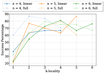
(a) Success probability out of 30 runs for different k-locality.

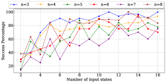
(b) Success probability out of 10 runs for different number of states used as input.

Figure 4: Experimental results for determining the k-locality and the amount of data (number of input states) required for successful compilation (a) The number of $k$-local Pauli observables required to distinguish between the different types of entanglement. We take the 4-,5-, and 6-qubit HEA with linear and full entanglement and run the compilation routine for each $k\in\{1,..,n\}$, where $n$ is the number of qubits under consideration, with 30 experiments each. The solid line shows the trend for linear entanglement, and the dashed line for full entanglement. (b) We fix $k=\lceil n/2\rceil$ and use HEA with linear entanglement. Successful compilation for any $n$-qubit can be achieved by using a number of states which gives the highest success probability according to the plot.

V Experiments

In this section, we will numerically evaluate QWC and benchmark it against HST and LET, focusing on each method’s demand for training data and susceptibility to barren plateaus. In all experiments, we are using the same parameterized quantum circuit as target and ansatz, each instantiated with different random parameters. Hence, the target $V$ is guaranteed to be in the unitary space representable by the ansatz $G(\bm{\theta})$, i.e. $\overline{F}(V,G(\bm{\theta}^{\star}))=1$ for all experiments. In all experiments, we utilized the ADAM optimizer with a learning rate of 0.1 for QWC and 0.04 for LET(HST), and exponential decay rates for the first and second moment estimates set as $\beta_{1}=0.9$ and $\beta_{2}=0.999$, respectively.

V.1 Hyperparameters

Our compilation routine consists of the generator and the discriminator, each requiring hyperparmeters related to the respective cost functions. We introduced the need for a test state ensemble for FUMC, i.e. a set $\mathcal{A}$ of quantum states which are used to calculate the empirical cost $\tilde{C}_{QW}^{(k)}(U,V,\mathcal{A})$. The question then arises about the cardinality of this set and whether the set should be dynamically changed over the course of the training. We also define successful compilation in terms of the cost function, whenever the cost function is below $10^{-3}$. We found from our initial experiments that using a fixed set of states already gives successful training curves. This observation can also be interpreted as a test whether our set is large enough. For the discriminator, we mentioned that the expectation value of the Hamiltonian Eq. (16) needs to be evaluated for a $k$-local Pauli string. $k$ is another hyper-parameter which needs to be tuned according to the problem. We show in Fig. 4a the success percentage over 30 experiments of compilation of a $4,5$ and $6$-qubit HEA target ansatz pair, against the $k$-locality used to detect the entanglement in the target for two cases, linear and full entanglement. The two entangling circuits are shown in Fig. 3. We see a general trend of higher $k$ having higher success probability. Yet, a larger $k$ also means many observables for computation. We choose to scale $k$ with $n$ as $k=\lceil n/2\rceil$.

V.2 Data Demand

After choosing the $k$-locality for the discriminator and choosing a fixed state set $\mathcal{A}$, we conducted experiments to determine the number of states needed to achieve successful compilation. For number of qubits $n\in\{3,...,8\}$ we ran the training for $|\mathcal{A}|\in\{2,...,16\}$ and calculated the fraction of runs which were successful out of a total of 10 runs for each state. We show the results in Fig. 4b. We see the general trend that the success percentage increases as we increase the number of states used, which is what we expect. Yet, a higher number of states also requires higher computation time, and thus we must balance between successful compilation and amount of compute. For the rest of the experiments we chose the state set size $|\mathcal{A}|=8$ for both QWC and LET.

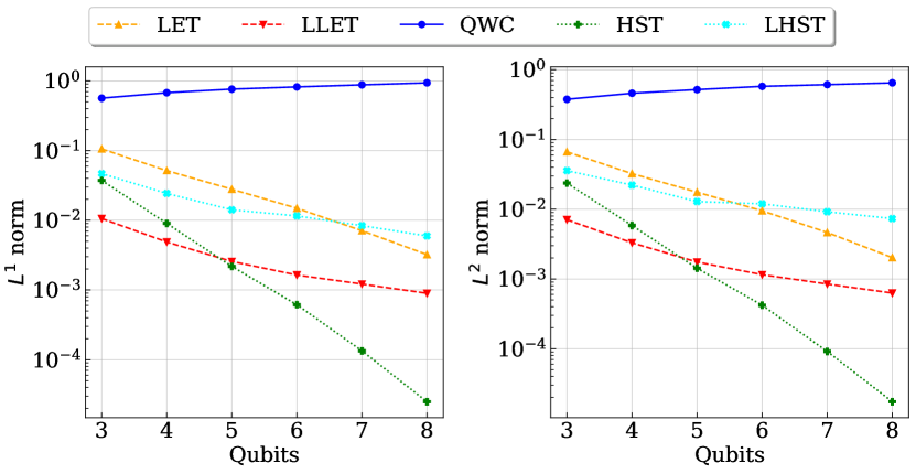
Figure 5: $l^{1}$-norm and $l^{2}$-norm of the gradient of the three cost functions against the number of qubits. The gradient is taken of the first parameter update step. Each point corresponds to the average over 100 runs.

V.3 Mitigating Barren Plateaus

To demonstrate that QWC can mitigate the barren plateaus in the optimization landscape, we plot the $l^{1}$-norm and $l^{2}$-norm of the gradient of the cost function with respect to the parameters of the ansatz, against the number of qubits in the circuit. We follow the same approach as [6] and calculate the gradients at the first optimization step. As before we work with HEA as both target and ansatz, having linear entanglement, restricting the Pauli observables set to $k=\lceil n/2\rceil$-locality and $|\mathcal{A}|=8$ for all the qubits. The results are shown in Fig. 5. We can see that the gradient norms of LET and HST decrease drastically as the number of qubits increases, indicating the presence of barren plateaus. In contrast, the gradient norms of QWC remain relatively constant, suggesting that the optimization landscape of QWC is not affected by the barren plateaus.

V.4 Training results

The cost function Eq. (12) is the metric we use in training our generator and discriminator, where as we reduce the cost $C_{QW}$ we are guaranteed that the infidelity between the test states decreases as well, and the generator learns to mimic the target unitary. We show the infidelity vs. inverse training error $C_{QW}^{-1}$ for 3 and 4-qubit circuits in Fig. 6a and 6b. We let the training run for $1000$ steps and we see that our cost function can reach values down to $10^{-16}$ in the infidelity, which is comparable to both LET and HST. Since such high precisions are usually not required in practical compilation routines, we plot in Fig. 7 the same plots for $n\in\{5,..,8\}$ but with early-stopping. The early-stopping condition is invoked whenever the variance of the cost function in the last $100$ steps is less than $10^{-8}$. Both LET and HST reach convergence faster than our cost function and they also have higher success rates compared to our method. In  8 we plot the training curves for $n=4,6$ qubits to show convergence.

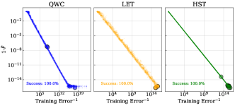
(a) $n=3$

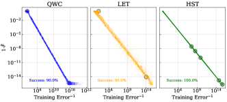
(b) $n=4$

Figure 6: Final infidelity ($1-\bar{F}$) vs. inverse training error ($C_{QW}^{-1})$ for hardware efficient ansatz (HEA) with full entanglement for $n=3$ and $n=4$ qubits. The training is carried out for 1000 steps. A run is successful when the cost function is below the threshold of $10^{-3}$. We see the trend that QWC like the other cost functions reaches extremely low values with a high probability.

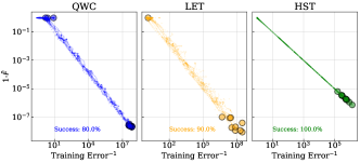
(a) $n=5$

(b) $n=6$

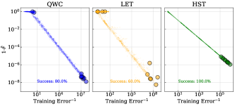
(c) $n=7$

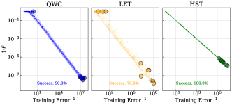
(d) $n=8$

Figure 7: Final infidelity ($1-\bar{F}$) vs. inverse training error ($C_{QW}^{-1})$ for hardware efficient ansatz (HEA) with full entanglement for $n\in\{5,..,8\}$. Since most applications do not require infidelity values of order $10^{-15}$, here we employ early stopping of training when the variance of last 100 cost values reaches $10^{-8}$.

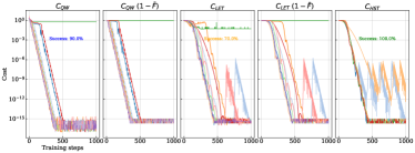
(a) $n=4$

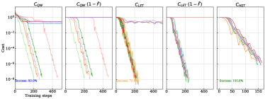
(b) $n=6$

Figure 8: Training curves for the 4-qubit and 6-qubit target ansatz pair for HEA with full entanglement. (a) Here the training is continued for the full 1000 steps in order to verify if all the methods reach the same global optimum. (b) Here early stopping is employed, where the training is stopped if the last 100 values of the variance of the cost function reaches $10^{-8}$. We see that in this case LET and HST reach convergence faster than QWC.

VI Conclusion

We have introduced a new cost function for VQCC based on the Wasserstein distance of order 1. This function leverages a quantum computer to estimate the similarity of two quantum circuits and integrates the concept of the Wasserstein distance, which is not unitarily invariant, in contrast to other commonly used distances.

We measure the similarity between two circuits, using three main aspects. Firstly, we estimate the Wasserstein distance between two quantum states. Since no efficient method for measuring or estimating the Wasserstein distance is currently known, we have adopted a method based on measuring local Pauli operators. We use the expectation values of these measurements in a linear program to construct an observable. The difference in the expectation values of this observable serves as our Wasserstein distance estimate. This estimation process functions as a discriminator—an agent that learns to distinguish between two states. It is countered by the variational circuit, or generator, which is trained to reduce the distance estimated by the discriminator. Thus, the PQC and distance estimator can be viewed as a generative adversarial network (GAN).

Building on this idea of quantum state learning, we have formulated a measure of similarity for two unitary transformations, termed the Wasserstein compilation cost function. This function is derived from the average Wasserstein distance over all states distributed according to the Fubini-Study measure. We provide an upper bound for the average infidelity of two unitary transformations in terms of this QWC cost function. This has led to the introduction of an empirically estimated Wasserstein compilation cost, obtained by measuring a few input states. The average Wasserstein distance of the resulting output states—those generated by the target unitary and the variational unitary from the respective input states—yields the empirical cost function used for circuit compilation. Hence, QWC can be considered an instance of a quantum circuit compilation GAN.

The circuit compilation is carried out on a quantum simulator for 3-8 qubit circuits. In our simulations, several key insights emerged. Firstly, the locality of the Pauli observables available to the discriminator significantly impacts its effectiveness. If the locality is too limited relative to the unitary’s complexity in terms of entanglement, the similarity is overestimated, leading to an unfaithful learning signal from the cost estimation. Moreover, the measurement effort for QWC was notably larger, with $\mathcal{O}(n^{k})$ observables required. A clear correlation was observed between the infidelity of the target state and the learned state, and their Wasserstein compilation cost, given a sufficiently large locality.

Secondly, the selection of sample states is critical for accurate estimation. Simulations demonstrated that simultaneous measurements on a fixed set of randomly sampled test states suffice to effectively learn a unitary. While the exact requirements for the training data remain an open question, Caro et al. [5] found that the number of states needed increases only polynomially with $n$. Comparative analysis of compilations for QWC, HST, and averaged LET revealed similar approximation results. Although HST outperformed our compilation cost for all qubits with a 100 % success rate, it quickly becomes impractical for larger number of qubits due to its requirement of twice the number of qubits for evaluation. The primary limitation of our method lies in the scaling of the measurement observable with the number of qubits, and future research will aim to enhance this efficiency.

Lastly, the numerical simulations in this study were conducted without considering noise. Sharma et al. [14] identified optimal parameter noise resilience for HST and LET. Future research will explore the noise resilience of QWC.

Appendix A Quantum $W_{1}$ distance and Fidelity

As explained in Section  II.1, the standard measure of success in variational quantum compilation is the average fidelity $\overline{F}(U,V)$, Eq. (2). Naturally, the question arises: what is the relation between the average quantum $W_{1}$ distance $C_{QW}(U,V)$ (Eq. 11) and $\overline{F}(U,V)$?

The starting point for our derivation is Proposition 2 of [16] that states upper and lower bounds for the quantum $W_{1}$ norm in terms of the trace norm $\lVert\cdot\rVert_{1}$.

$$\frac{1}{2}\lVert\rho-\sigma\rVert_{1}\leq\lVert\rho-\sigma\rVert_{W_{1}}\leq\frac{n}{2}\lVert\rho-\sigma\rVert_{1}$$ (23)

Additionally, the trace norm is bounded by the fidelity $F(\rho,\sigma)$:

$$1-\sqrt{F(\rho,\sigma)}\leq\frac{1}{2}\lVert\rho-\sigma\rVert_{1}\leq\sqrt{1-F(\rho,\sigma)}.$$ (24)

Hence, we can find a lower bound for the fidelity in terms of the quantum $W_{1}$ norm:

$$1-\lVert\rho-\sigma\rVert_{W_{1}}\leq\sqrt{F(\rho,\sigma)}.$$ (25)

Since the fidelity is bounded, $0\leq F(\rho,\sigma)\>\forall\>\rho,\sigma\in\mathcal{S(\mathcal{H})}$, the same holds for $\sqrt{F(\rho,\sigma)}$. We will now constrain the quantum $W_{1}$ norm to small values, $0\leq\lVert\rho-\sigma\rVert_{W_{1}}\leq 1$. This domain is of particular interest as we formulate the VQC problem as a minimization of the quantum $W_{1}$ norm. With this constraint, we can square the inequality and make use of Bernoulli’s inequality:

$$F(\rho,\sigma)\geq\left(1-\lVert\rho-\sigma\rVert_{W_{1}}\right)^{2}\geq 1-2\lVert\rho-\sigma\rVert_{W_{1}}.$$ (26)

By this bound, we now know that a vanishing Earth Mover’s distance between two mixed states translates to high fidelity of the states. But this result for mixed states only holds for small distances, e.g. $\lVert\rho-\sigma\rVert_{W_{1}}\leq 1$.

A more general result can be found for pure states. Note that quantum Wasserstein compilation actually uses pure states. For two pure states $\rho=\ket{\psi}\bra{\psi},\sigma=\ket{\phi}\bra{\phi}$, the following equality between trace norm and fidelity $F(\ket{\psi},\ket{\phi})=\lvert\braket{\psi}{\phi}\rvert^{2}$ holds:

$$\big{\lVert}\ket{\psi}\bra{\psi}-\ket{\phi}\bra{\phi}\big{\rVert}_{1}=\sqrt{1-F(\ket{\psi},\ket{\phi})}.$$ (27)

Using again Eq. (23), we bound the fidelity by the quantum $W_{1}$ norm

$$\big{\lVert}\ket{\psi}\bra{\psi}-\ket{\phi}\bra{\phi}\big{\rVert}_{W_{1}}\geq\sqrt{1-F(\ket{\psi},\ket{\phi})}$$ (28)

and square without further constraints

$$\big{\lVert}\ket{\psi}\bra{\psi}-\ket{\phi}\bra{\phi}\big{\lVert}_{W_{1}}^{2}\geq 1-F(\ket{\psi},\ket{\phi}).$$ (29)

This upper bound for the infidelity of pure states in terms of the quantum $W_{1}$ norm will motivate our definition of the Wasserstein compilation cost.

Appendix B Gradients of the Empirical Cost Function

In Section IV.2, we defined the cost function to estimate the restricted quantum EM distance (Eq. 18). Since we focus only on gradient based optimization routines, we derive the derivative of the cost function $\tilde{C}_{QW}(U,V(t),\mathcal{A})$, here written for a single parameter $t$.

Proposition 4.

Let $V$ be a unitary operator of $\mathcal{H}$ and $U(t)$ a parametric family of unitary transformations of $\mathcal{H}$. Then, the derivative of the empirical Wasserstein compilation cost in parameter $t$ can be expressed as

$$\begin{split}\diff*{\tilde{C}_{QW}(U(t),V,\mathcal{A})}{t}[t=0]&\\ =\sum_{\psi\in\mathcal{A}}\frac{2}{|\mathcal{A}|}W_{1}\Bigl{(}U(0)\ket{\psi},V\ket{\psi}\Bigr{)}&\\ W_{1}^{\prime}\Bigl{(}U(0)\ket{\psi},V\ket{\psi}\Bigr{)}\end{split}$$ (30)

where $\mathcal{A}$ is the set of probe states and $W_{1}^{\prime}$ can be calculated according to Eq. (20).

Proof.

The proof follows by simply applying the sum rule and the chain rule for derivative:

$$\diff*{\tilde{C}_{QW}(U(t),V,\mathcal{A})}{t}[t=0] = \diff*{\frac{1}{|\mathcal{A}|}\sum_{\psi\in\mathcal{A}}W_{1}^{2}\Bigl{(}U(t)\ket{\psi},V\ket{\psi}\Bigr{)}}{t}[t=0]=\frac{1}{|\mathcal{A}|}\sum_{\psi\in\mathcal{A}}\diff*{W_{1}^{2}\Bigl{(}U(t)\ket{\psi},V\ket{\psi}\Bigr{)}}{t}[t=0]$$

$$= \sum_{\psi\in\mathcal{A}}\frac{2}{|\mathcal{A}|}W_{1}\Bigl{(}U(0)\ket{\psi},V\ket{\psi}\Bigr{)}\diff*{W_{1}\Bigl{(}U(t)\ket{\psi},V\ket{\psi}\Bigr{)}}{t}[t=0]$$

∎

References

- Preskill [2018] J. Preskill, Quantum Computing in the NISQ era and beyond, Quantum 2, 79 (2018), arxiv:1801.00862 .
- Khatri et al. [2019] S. Khatri, R. LaRose, A. Poremba, L. Cincio, A. T. Sornborger, and P. J. Coles, Quantum-assisted quantum compiling, Quantum 3, 140 (2019), arxiv:1807.00800 .
- Cincio et al. [2018] L. Cincio, Y. Subaşı, A. T. Sornborger, and P. J. Coles, Learning the quantum algorithm for state overlap, New Journal of Physics 20, 113022 (2018).
- Cincio et al. [2021] L. Cincio, K. Rudinger, M. Sarovar, and P. J. Coles, Machine Learning of Noise-Resilient Quantum Circuits, PRX Quantum 2, 010324 (2021).
- Caro et al. [2022] M. C. Caro, H.-Y. Huang, M. Cerezo, K. Sharma, A. Sornborger, L. Cincio, and P. J. Coles, Generalization in quantum machine learning from few training data, Nature Communications 13, 4919 (2022).
- Kiani et al. [2022] B. T. Kiani, G. De Palma, M. Marvian, Z.-W. Liu, and S. Lloyd, Learning quantum data with the quantum earth mover’s distance, Quantum Science and Technology 7, 045002 (2022).
- Cerezo et al. [2021a] M. Cerezo, A. Arrasmith, R. Babbush, S. C. Benjamin, S. Endo, K. Fujii, J. R. McClean, K. Mitarai, X. Yuan, L. Cincio, and P. J. Coles, Variational quantum algorithms, Nature Reviews Physics 3, 625 (2021a).
- Holmes et al. [2022] Z. Holmes, K. Sharma, M. Cerezo, and P. J. Coles, Connecting ansatz expressibility to gradient magnitudes and barren plateaus, PRX Quantum 3, 010313 (2022), arxiv:2101.02138 [quant-ph, stat] .
- Mele et al. [2022] A. A. Mele, G. B. Mbeng, G. E. Santoro, M. Collura, and P. Torta, Avoiding barren plateaus via transferability of smooth solutions in Hamiltonian Variational Ansatz, Physical Review A 106, L060401 (2022), arxiv:2206.01982 [quant-ph] .
- Bilkis et al. [2023] M. Bilkis, M. Cerezo, G. Verdon, P. J. Coles, and L. Cincio, A semi-agnostic ansatz with variable structure for quantum machine learning (2023), arxiv:2103.06712 [quant-ph, stat] .
- Cerezo et al. [2021b] M. Cerezo, A. Sone, T. Volkoff, L. Cincio, and P. J. Coles, Cost function dependent barren plateaus in shallow parametrized quantum circuits, Nature Communications 12, 1791 (2021b).
- Nielsen [2002] M. A. Nielsen, A simple formula for the average gate fidelity of a quantum dynamical operation, Physics Letters A 303, 249 (2002), arxiv:quant-ph/0205035 .
- Goussev et al. [2012] A. Goussev, R. A. Jalabert, H. M. Pastawski, and D. Wisniacki, Loschmidt Echo, Scholarpedia 7, 11687 (2012), arxiv:1206.6348 [cond-mat, physics:quant-ph] .
- Sharma et al. [2020] K. Sharma, S. Khatri, M. Cerezo, and P. J. Coles, Noise resilience of variational quantum compiling, New Journal of Physics 22, 043006 (2020).
- Wilde [2017] M. Wilde, Quantum Information Theory, second edition ed. (Cambridge University Press, Cambridge, UK ; New York, 2017).
- De Palma et al. [2021] G. De Palma, M. Marvian, D. Trevisan, and S. Lloyd, The Quantum Wasserstein Distance of Order 1, IEEE Transactions on Information Theory 67, 6627 (2021).
- De Palma et al. [2022] G. De Palma, M. Marvian, C. Rouzé, and D. S. França, Limitations of variational quantum algorithms: A quantum optimal transport approach (2022), arxiv:2204.03455 [quant-ph] .
- McClean et al. [2018] J. R. McClean, S. Boixo, V. N. Smelyanskiy, R. Babbush, and H. Neven, Barren plateaus in quantum neural network training landscapes, Nature Communications 9, 4812 (2018).
- Grant et al. [2019] E. Grant, L. Wossnig, M. Ostaszewski, and M. Benedetti, An initialization strategy for addressing barren plateaus in parametrized quantum circuits, Quantum 3, 214 (2019), arxiv:1903.05076 .
- Schuld et al. [2018] M. Schuld, V. Bergholm, C. Gogolin, J. Izaac, and N. Killoran, Evaluating analytic gradients on quantum hardware, arXiv:1811.11184 [quant-ph] 10.1103/PhysRevA.99.032331 (2018), arxiv:1811.11184 [quant-ph] .
- Caro et al. [2023] M. C. Caro, H.-Y. Huang, N. Ezzell, J. Gibbs, A. T. Sornborger, L. Cincio, P. J. Coles, and Z. Holmes, Out-of-distribution generalization for learning quantum dynamics, Nature Communications 14, 3751 (2023).
- Sharma et al. [2022] K. Sharma, M. Cerezo, Z. Holmes, L. Cincio, A. Sornborger, and P. J. Coles, Reformulation of the No-Free-Lunch Theorem for Entangled Datasets, Physical Review Letters 128, 070501 (2022).
- Poland et al. [2020] K. Poland, K. Beer, and T. J. Osborne, No Free Lunch for Quantum Machine Learning (2020), arxiv:2003.14103 [quant-ph] .
- Lloyd and Weedbrook [2018] S. Lloyd and C. Weedbrook, Quantum Generative Adversarial Learning, Physical Review Letters 121, 040502 (2018).