Enhancement of fusion reactivities using non-Maxwellian energy distributions
Abstract
We discuss conditions for the enhancement of fusion reactivities arising from different choices of energy distribution functions for the reactants. The key element for potential gains in fusion reactivity is identified in the functional dependence of the tunnellng coefficient upon the energy, ensuring the existence of a finite range of temperatures for which reactivity of fusion processes is boosted with respect to the Maxwellian case. This is shown, using a convenient parameterization of the tunneling coefficient dependence upon the energy, analytically in the simplified case of a bimodal Maxwell-Boltzmann distribution, and numerically for kappa-distributions, We then consider tunneling potentials progressively better approximating fusion processes, and evaluate in each case the average reactivity in the case of kappa-distributions.
I Introduction
The relevance of controlled nuclear fusion in the current context, to contain global warming and to mitigate geopolitical conflicts, has been extensively debated. While the gap between experimental demonstrations and commercial use of nuclear fusion is being progressively narrowed with projects like ITER currently under construction, and DEMO, in the middle of this century, there have been parallel efforts to discuss the possibility to enhance fusion cross-sections by exploiting the basic physics of tunneling and the possible presence of screening of the Coulomb barrier. Considering the extreme sensitivity of quantum tunneling to the details of the process, significant gains may be expected. Examples of proposals range from discussion of correlated states Vysotskii , interference from superposition of plane waves Ivlev , use of generalized Gaussian wave packets Dodonov1 ; Dodonov2 , shielding of strong electromagnetic fields Lv , the effect of the hypothetical presence of strong scalar fields Zhang , among the many proposals. Another sequel of proposals has been focused on the intrinsic three-dimensional nature of the confined plasmas, with the goal to enhance the reactivity by producing Maxwell-Boltzmann (MB) distributions with different temperatures along different spatial directions Harvey1986 ; Nath2013 ; Kolmes2021 ; Li et al. (2022); Xie2023a ; Xie2023b .
In this paper we discuss the impact of various choices of macroscopic states for the reactants, i.e. their energy distribution, on the resulting average reactivity. Preliminary discussions of this aspect can be found in Majumdar2016 using Dagum distributions, and in Onofrio , in which the potential gain in using energy distributions with hard high-energy tails of the so-called kappa distributions (-distributions in the following) – already broadly used in space plasma physics and astrophysics Livadiotis2011 ; Nicholls1 ; Nicholls2 ; Livadiotisa – has been discussed by evaluating reactivities with empirically determined fusion cross-sections Bosch . We extend here these considerations to analytically evaluated ab initio cross-sections, showing general features and discussing conditions under which gains are expected with respect to Maxwell-Boltzmann (MB) energy distributions. A recent paper is also exploring, on top of trapping anisotropies, -distributions in magnetically confined plasmas Kong2024 .
The paper is organized as follows. In section II we first recall general properties of two classes of non-MB distributions, bimodal MB and -distributions. We discuss the presence of population excesses at low and high energy, and population depletion at intermediate energies with respect to a Maxwell-Boltzmann distribution. We then report, in Section III, average reactivities gains in an idealized case of tunneling coefficient dependence upon the energy. In section IV we discuss tunneling in the case of two barriers which are amenable to a complete analytic treatment, yet capturing some features of the more complex nuclear fusion case, the double square well and a generalized form of the Wood-Saxon potential. In the same section we also provide explicit examples of configurations, within these two classes of potentials, for which it is advantageous to use -distributions. We briefly comment on the impact for fusion reactions involving deuterium-deuterium and deuterium-tritium mixtures, by using empirical cross-sections already available in the literature.
In the conclusions we qualitatively comment on the potential relevance of these results in the context of magnetic confined fusion reactors. Two appendices, one on explicit calculations for the tunneling coefficient of the square well case, and another on the discussion of the convexity of the tunneling coefficient evaluated with the WKB (Wentzel-Kramers-Brilllouin) approximation in the case of two relevant barriers, complete the paper.
II Generalized energy distributions
In practical settings and especially in hot plasmas, the energy distributions of the reactants is determined by classical statistical mechanics. We will discuss here two energy distributions more general than the MB energy distribution, namely a superposition of two MB distributions at different temperatures, and the so-called -distribution.
The MB in one dimension is defined as
| (1) |
with , the unique parameter of this energy distribution, being the inverse temperature, such that the temperature is related to as , with the Boltzmann constant, and expressed in Kelvin. A bimodal Maxwell-Boltzmann distribution (bMB) is described by the weighted sum of two MB distributions
| (2) |
Here the two weights and satisfy , and the average energy of a bimodal system is . We therefore can compare a bMB distribution to a single MB distribution with the same average energy, which means with a MB distribution with inverse temperature such that
| (3) |
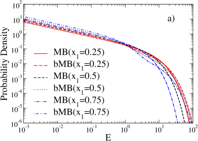
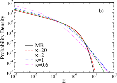
Examples of bMB energy distributions and comparison to the corresponding MB distributions with the inverse temperature determined by Eq. (3) are shown in Fig. 1a. Actual bMB distributions have been observed in laboratory plasmas Bhatnagar1993 .
The class of distributions was introduced to fit magnetospheric electron data, and have been used to describe a plethora of astrophysical and space plasmas phenomena Livadiotisa . It has been also discussed in the framework of nonextensive statistical mechanics in which the -parameter, representing non-extensivity, is shown to be related to the -parameter Tsallis2009 . Moreover, it has been shown that generalizations of bMB distributions allow to effectively capture the effect of a -distribution Hahn2015 . In the one-dimensional case, -distributions can be expressed, as discussed in Vrinceanu , in the following form
| (4) | |||||
in which, in addition to the inverse temperature , two further parameters appear with respect to a MB distribution, and . The parameter expresses the ‘distance’ of the distribution from the corresponding MB distribution, and determines more specifically the high-energy behaviour due to its presence in the generalized, power-law dependent, Lorentzian function. Based on the usual definition of the exponential function as a limiting process , it is evident that the MB distribution in Eq. (1) is recovered for .
For finite instead the distribution has larger probability in the high energy tail with respect to the corresponding MB distribution, and these hard tails become more prominent as becomes smaller. The average energy of a particle in a -distributed ensemble is written as
| (5) | |||||
where the dimensionless parameter is defined as . Equation (5) shows that the expectation of the equipartition principle valid for a MB distribution in one-dimension () is modified by a factor , obviously tending to unity for , the MB limit. For the choice , the kinetic definition of temperature valid for a MB distribution is recovered regardless of the value of , allowing for a fair comparison between different -distributions therefore having the same total energy. This also coincides with the dependence of on the number of kinetic degrees of freedom of the system (in our case ), as Livadiotisb . A comparison between and MB distributions is also possible in general at the price however of introducing an effective temperature depending on . For this reason, we will focus in the following considerations only on the simplest case of .
Some remarks are also in order. First, the parameters and can be related to the velocity distribution’s second moment
| (6) |
showing that both and are related to the distribution’s variance (since the average velocity is zero), with the exceptional case of commented above.

Second, the velocity distribution corresponding to the energy distribution as in Eq. (4), expressed as
| (7) | |||||
always reaches a maximum at , and the ratio between the peaks of -distribution and the corresponding MB distribution for is
| (8) |
By using asymptotic expressions for the Gamma-function, for instance a Stirling-like formula (see more in general Xu )
| (9) |
we find that in the case we are considering, the ratio in Eq. (8) is always larger than unity for a finite , obviousy tending to unity in the limit. This implies that -distributions have both hard high energy tails and more populated peaks at zero velocity with respect to the corresponding MB distribution. Due to the normalization of probability distributions, this implies that there will be an intermediate regime of velocities in which the MB distribution prevails over the -distribution. This effect is shown in Fig. 1b, in which various -distributions are considered including the limiting case of a MB distribution, nearly indistinguishable from a -distribution for .
Third, an intriguing situation occurs in the limit of , as in this case, by introducing such that , we have
| (10) | |||||
which, for and in the specific case of we are considering, can be written as
| (11) |
diverging in the limit of at finite .
III Reactivity with non-MB distributions
In this section we provide more quantitative arguments for understanding the effectiveness of the non-Boltzmann distributions with respect to a MB distribution (for previous related discussions see also Onofrio ; Vrinceanu ) for processes involving tunneling phenomena, such as fusion. Before discussing the results, it is worth to comment on this specific, unusual situation, in which the velocity (and kinetic energy) distribution is dominated by classical physics, yet the reactants are evolving with fully quantum mechanical laws, either via Rutherford scattering (ineffective for nuclear fusion) or via fusion allowed by quantum tunneling. This implies that the variance of the single wave packet, so far considered as attributable to a Gaussian momentum distribution as customary for wave packets of quantum mechanical origin, is actually determined by the spreading of the velocities due to the classical distribution in the statistical ensemble, which in turn depends on temperature and density and the and parameters in the case of a -distribution (for a related discussion see Kadomtsev1997 ). The cross-section corresponding to the tunneling process is
| (12) |
where we have introduced the wave vector such that , and the velocity of the particle with wave vector is . The average reactivity is then calculated as
Basically the potential gain in using non-Boltzmann distributions stems from the fact that, with respect to a MB distribution, there is a more populated high energy tail. For the same average energy, this means that the non-Boltzmann distribution will also have a more populated low energy component, as visible in Fig. 1. Then the advantage on using non-Boltzmann distributions relies on the functional dependence of the tunneling probability upon the energy, . If the latter is a convex function, the contribution to the integrated tunneling probability from the high-energy tail will overcompensate the lower contribution due to the increased component of the distribution at low energy. We also expect that at temperature large enough there will be marginal gain in using non-Boltzmann distributions. Indeed, for an arbitrary barrier we have for , which implies that at high energy curve will always be concave. We therefore mainly focus on the behavior at lower temperatures, which is also the most interesting region for fusion reactions of technological interest.
For a generic non-MB distribution the gain with respect to the corresponding MB distribution may be quantified by considering the difference between the reactivities defined as
| (14) |
A more practical and universal dimensionless parameter is obtained by considering , the relative deviation from the MB reactivity.
In a hypothetical case of scaling exactly as in the entire energy range, this difference will be zero, as the two distributions are normalized to unity. However the tunneling coefficient cannot grow indefinitely, being limited to unity, so this scaling law does not allow for break-even in practice. The difference , for the two cases of non-MB distributions we are considering, is positive at low and high energy, being instead negative in a regime of intermediate energies, as already commented. However, at low energy the tunneling coefficient is small, while at high energy the cross-section is small as evident by the explicit factor, with the tunneling coefficient approximating unity.
In order to put the discussion on a more quantitative ground, we introduce a fictitious tunneling coefficient depending on the energy as
| (15) |
The parameter () plays the role of a ‘convexity’ parameter such that for we have convex if , concave if .
This allows to obtain a simple relationship for in the case of bMB distributions. In this case the reactivity difference is written as
| (16) | |||||
where
| (17) | |||||
with , and
| (18) |
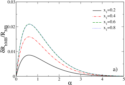
is the incomplete Gamma function of order . In Fig. 2 we show the plots of versus for various values of , for a bMB distribution. The case (a) is relative to a choice of , case (b) deals with the opposite situation of . In the limit , , the complete Gamma function, and then in the same limit there is complete cancellation among the three contributions, with the plot showing the small, residual term at finite . In the opposite limit, , the second term in the righthandside of (17) tends to zero, and then . This implies a limit form of the reactivity relative difference
| (19) |
It is easy to check that for , , and for , , with the bordeline case yielding . Therefore it is confirmed, at least for this power-law dependence of the tunneling coefficient upon the energy, that a convex function yields gain in using a bMB distribution with respect to a MB distribution with the same average energy. Considering the richness of possible situations, both in terms of dependences, with the possibility of resonant tunneling for instance, and of possible non-Maxwellian distributions, this result has to be considered a qualitative guideline to appreciate the possibility of reactivity gains in a general context.
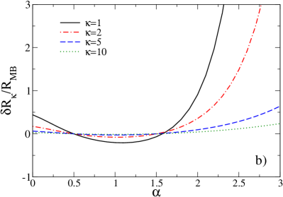
In the case of distributions, we write an analogous relationship
| (20) |
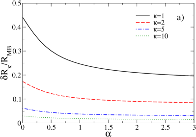
and the numerical integration provides the plots in Fig. 3 once again for choices of (a) and (b). Similarly to the bMB case, when is small there is a small enhancement at all , due to the low-energy dominance of the distribution with respect to the corresponding MB distribution. The case of large is more interesting showing an interval of values for which the reactivity of the MB distribution is significantly larger than the one of the distribution, which instead prevails at small and large . The enhancement strongly depends on , and large values of this parameter, either a large or a low temperature , makes the reactivity quite sensitive to the high-energy tails, more prominent in the -distribution than in the MB case. Also notice that, unlike the case of the bMB distribution, the threshold value of for which the distribution has higher reactivity occurs at , therefore requiring more curvature due to the presence of a strong low-energy component in the -distribution and a stronger depletion at intermediate energies, as noticeable by comparing the two panels of Fig. 1.
In the specific case of a -distribution with discussed earlier, it is possible to support a similar convexity argument as follows. The reactivity in that case assumes the form
| (21) |
where is the tunneling coefficient expressed as a function of the particle velocity, , and we expect for . This means that the reactivity does not present divergences at large velocities. However there are possible divergences in the limit, depending on . Let us focus on the integrand at small , including also the infinitesimal quantity for the analysis of the divergences. Let us suppose that , i.e. goes to zero as the velocity, with a characteristic velocity, for instance the quadratic mean velocity. Then we will have an expression for the reactivity as
| (22) |
Suppose that in the limit, then , which means that the integral will be finite if , and diverging at otherwise. This confirms, within the limit of this example and related assumptions, that the dependence should correspond to a convex function at least initially to avoid meaningless divergences of the reactivity. Notice that in this case the reactivity is directly proportional to the temperature.
IV Tunneling coefficients for potentials with analytic solutions of the Schroedinger equation
In this section, we discuss tunneling probabilities for one-dimensional systems described by potentials progressively approximating the physical case of nuclear fusion but still admitting analytical solutions. We start by considering the case of a potential describing a stepwise double symmetric barrier, then we discuss the most realistic case of a generalized Wood-Saxon potential. We investigate the tunneling phenomenon for different preparations of the wavefunction of the incident particle. As discussed in OnofrioPresilla , there is a sensitive dependence of the tunneling coefficient upon the spatial spreading of the incident wavepacket. While we refer to this contribution for further details, we summarize here the results relevant for the current discussion.
The incident particle is schematized via a Gaussian wavepacket with positional spreading (such that the position variance is ), average wave vector and mean energy :
| (23) |
The corresponding wavefunction in wave vector space is
| (24) | |||||
Therefore the probability to measure a generic wave vector is a Gaussian function of peaked around
| (25) |
The tunneling coefficient is therefore expressed by an integral over all wave vectors as
| (26) |
The reactivity is evaluated as
| (27) | |||||
where if the energy is -distributed () we have
| (28) | |||||
while in the MB case (=MB) we have
| (29) |
As discussed in OnofrioPresilla , the reactivity for fusion processes is extremely sensitive to the spreading of the Gaussian wavepacket, reaching a maximum for an intermediate value of . We will discuss in the following both cases of highly localized Gaussian wavepackets as well as states resembling the limiting case of plane waves. Besides extending the analysis to localized states, we introduce now more realistic potentials leading to tunneling processes, in lieu of considering an artificial case as the one of Eq. (15). We first consider a stepwise double barrier potential defined as
| (30) |
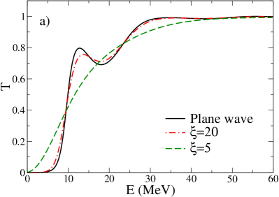
where and e are both positive defined. If the potential becomes a double barrier surrounding a well of depth . This potential admits an analytic solution for the corresponding time-independent Schroedinger equation, and transmission and reflection coefficients are calculated as described in detail in Appendix A. In plot (a) of Fig. 4 the dependence of the tunneling coefficient upon the energy of an incident particle is shown for two cases of positional spreading , and of a plane wave. A distinctive feature of the various cases is that for large positional spreading the curvature of the tunneling coefficient is positive at low energy, i.e. is initially a convex function. For small positional spreading the curve becomes concave in the whole range except in a tiny region near .
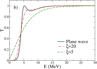
A more realistic case, at least because of the absence of discontinuities, is provided by the Generalized Woods-Saxon (GWS) potential energy for a one-dimensional system as first discussed in Luftuglu2016
| (31) |
parameterized by two characteristic lengths, and , and two energy scales, and . The parameter determines the size of the effective well, and is its spatial spread. The potential has a value in the origin equal to , while at . At large distances the potential energy decreases as . This means that a semiqualitative difference from potential energies of interest in nuclear fusion is that the barrier experienced by the nucleons, if schematized with this potential, does not have the long range as expected for Coulomb interactions, although in a realistic plasma the latter are screened on the Debye length. We choose the set of parameters as described in the caption of Fig. 4, resulting in well depth, barrier height and width of the well comparable to the ones of light nuclei.
These potentials are reminiscent, in a one-dimensional setting, of the more general nucleus-nucleon interaction potential which also includes a Coulomb term inside the nucleus dictated by an assumed uniform electric charge density (here neglected) and a centrifugal term with the possibility for a scattering with non-zero impact parameter evidently absent in an one-dimensional analysis, see for instance Bekerman1988 ; Vanderbosch1992 ; Balantekin1998 . The tunneling coefficient versus the energy of the incident particle is shown in plot (b) of Fig. 4 for different values of . A similar phenomenon to the case of a stepwise double well is also visible, with the change of convexity depending on the values of . The presence of less defined boundaries with respect to the stepwise case makes resonant tunneling less remarkable especially in the case, with a barely visible peak around the energy of 6 MeV.
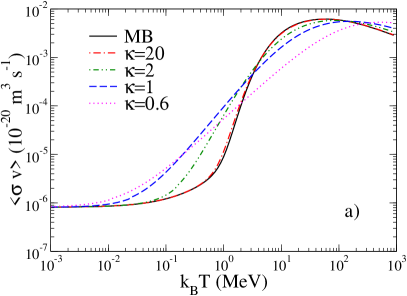
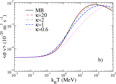
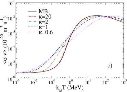
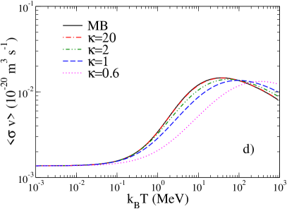
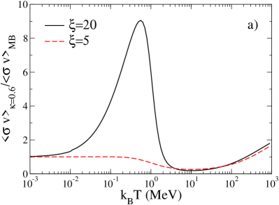
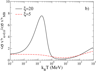
Based on these tunneling coefficients, we can evaluate the reactivities in some examples, for simplicity limiting the analysis to the case of -distributions. Representative results for the reactivity dependence upon the temperature are shown in Fig. 5 for both stepwise and GWS potentials. As for the tunneling coefficients, cases of Gaussian states with narrow and broad positional spreading are considered. A broad Gaussian state, with the transmission coefficient having positive curvature at low energy as shown in Fig. 4, at low temperature has a smaller reactivity for an MB distribution with respect to the corresponding -distribution. The opposite occurs in the case of a narrow Gaussian state in which the transmission coefficient has negative curvature in the entire range of energies. By increasing the temperature, the MB state dominates over the -distribution cases, until the harder energy tails of the latter determine once again a gain in reactivity at even higher temperatures. In order to better evidence the enhancement and suppression patterns, we show in Fig. 6 the ratio of reactivities between the case of , the most extreme -distribution we consider, and the case of the corresponding MB distribution. It is worth noticing that using broad Gaussian states with -distributions at small allow for a gain, with respect to the MB distribution, of almost one order of magnitude, and most importantly in a range of temperatures below 1 MeV, of relevance for nuclear fusion. The analysis seems robust with respect to the choice of the potential energy, as shown by the similarity of the curves in the two cases considered.
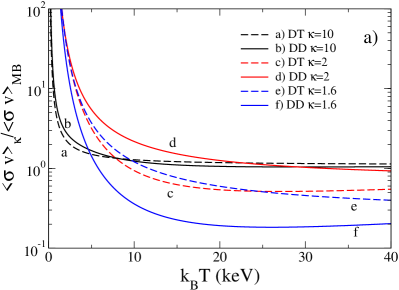
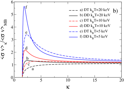
While we plan to discuss a comprehensive analysis of realistic cases of fusion in the future, it may be worth to briefly discuss the reactivity gain in using -distributions with respect to the MB case, evaluated from empirical cross-sections for fusion of deuterium-deuterium and deuterium-tritium mixtures Bosch . In Fig. 7 (a) this gain is plotted versus temperature in a range of interest for most of the experiments using Tokamak machines. The behavior is similar for the two mixtures. At large , as the case, there is no gain at high temperature, while in the same temperature range it is not advantageous to use energy distributions with smaller values of . Significant gains are instead expected at lower temperatures. In this region of temperature there is an optimal, intermediate value of maximizing the reactivity, since a too small creates a nearly diverging population at very low energy – see discussion around Eq. (11) – not favourable for fusion processes, see Fig. 7 (b). Optimizing the value of yields significant reactivity gains at low and already accessible temperatures. These gains could be even substantial because in this analysis we do not consider the optimization with respect to the positional spreading. Moreover, the interval of energies for which the reactivity is evaluated is limited by the parameterization to a finite range, thereby resulting in conservative estimates, considering the importance of the high-energy tail for the more populated -distribution. This analysis, based on a concrete three-dimensional situation, also confirms the general trends reported earlier on more idealized and one-dimensional models.
V Conclusions
By using generalizations of the Maxwell-Boltzmann statistics, we have discussed a key condition to enhance the tunneling probabilities and the reactivities of nuclear fusion processes in the framework of one-dimensional potentials admitting exact solutions for the corresponding time-independent Schroedinger equation. A prominent convexity of the transmission coefficient ensures that the unavoidable overpopulation of low energy states does not offset the effect of the high-energy tail in a -distribution, resulting in enhanced integrated reactivity with respect to the Maxwell-Boltzmann energy distribution operating at the same effective temperature. This has been explicitly shown for bMB and -distributions by using a convenient parameterization of the tunneling coefficient, and discussing how the latter can be approximated in more realistic, but still analytically tractable, potentials exhibiting tunneling.
We have presented examples of potentials for which it is advantageous to use non-Boltzmann distributions to enhance fusion reactivity. The whole parameter space for which such an advantage exists can be explored via optimization of the reactivity ratio with respect to a few parameters, three in the case of the stepwise double barrier, and four in the case of the GWS barrier, for each temperature and positional spreading. The optimization is far more complex in terms of requested numerical resources by using a more realistic potential such as, for example, a combination of Wood-Saxon and Coulomb potentials. It should be kept in mind that an overall optimization of the reactivity is what is beneficial to boost the fusion rate, therefore there is a competition between the choice of the positional spreading and the -parameter. As noticeable by comparing side by side the panels in Fig. 5, even if the gain in using a small is smaller with respect to the choice of a large with the same in the low temperature range, the absolute reactivities are larger in the former case.
Generalizations to more realistic cases requires handling tunneling coefficients and incorporating the possible presence of states with non-zero angular momentum in a full three-dimensional treatment, as well as the effect of the confining potential on the energy distribution. The extent to which -distributions can be realized in concrete setups is still open, however it is expected that long-range interactions in a generic statistical system will show deviations from a Maxwell-Boltzmann distribution rigorously valid only for short-range interactions. This point is extensively discussed in Tsallis2009 and corroborated by numerical simulations in the case of the Hamiltonian mean-field model Konishi ; Antoni . Although we still lack evidence for -distributed energies in the case of genuine dynamical systems such as interacting classical gases, steps towards this direction are currently undergoing JauffredOnoSun2019 ; OnoSun2022 . On the experimental side, spectroscopy of the fusion reaction products is expected to provide precise assessments of the deviation from MB distributions, as recently discussed in Crilly2022 .
Appendix A Tunneling coefficient in a stepwise double well potential
We report here the results for a potential made of a double well, starting with the time-independent Schroedinger equation
| (32) |
for a one-dimensional stepwise potential as defined in Eq. (30). Equation (32) admits, for , a continuous and doubly degenerate spectrum. For each energy eigenvalue there are two eigenstates and with the positive wave vector defined as
| (33) |
By introducing the positive wave vectors in the regions at potentials and
| (34) |
the eigenstates can be expressed as
| (35) |
In this form the state describes the stationary state of a particle coming from with momentum . The normalization is chosen in such a way that the eigentates are orthogonalized with respect to the wave vector Landau1977
| (36) |
The particle is reflected or transmitted respectively with probability
| (37) |
The reflection and transmission amplitudes and are determined together with the coefficients , and by imposing the continuity of the eigenstates and their first derivatives in the discontinuity points of the potential. This leads to
| (38) |
where
| (39) | |||||
| (40) | |||||
The remaining coefficients are then determined as
| (41) | |||
| (42) | |||
| (43) | |||
| (44) |
Appendix B Influence of the shape of the barrier on the convexity of the tunneling coefficient
In this appendix we show with a representative example how the shape of the barrier strongly influences the reactivity gain, even within the WKB approximation for which the only relevant quantity is the area of the classically forbidden region. In the case of a rectangular barrier of height and thickness , with the particle mass and energy and respectively, the WKB approximation yields
| (45) |
which, in the limit , can be expanded as
| (46) |
a linear dependence on in the same limit, implying no initial curvature.
If we instead consider a case with a smoother barrier, such as the following containing a Coulomb-like component
| (47) |
we obtain, always in the WKB approximation
| (48) |
where is observed to be convex in the entire range . More specifically, in the limit, the transmission coefficient is approximated as
| (49) |
Notice the non-analytical dependence , which implies a very soft increase and therefore a positive curvature at small values of , i.e. is convex. This is easily interpreted in terms of the behavior of the barriers as the energy of the impinging particle is increased. In the case of the rectangular barrier the increase in energy results in a linear decrease of the area of the classically forbidden region, therefore implying a square root dependence for the argument of the integral in the exponent of the WKB relationship. Instead, in the case of the Coulomb potential the decrease of the area of the classically forbidden region when increasing has a stronger dependence on , at least initially. This creates convexity of at low energy. Under these conditions, as discussed in Section IV, spreading the energy distribution can be advantageous for enhancing the reactivity.
References
- (1) V. I. Vysotskii, M. V. Vysotskyy, and S. V. Adamenko, Formation and application of correlated states in nonstationary systems at low energies of interacting particles. J. Exp. Theor. Phys. 114, 243 (2012).
- (2) B. Ivlev, Low-energy fusion caused by an interference, Phys. Rev. C 87, 034619 (2013).
- (3) A. V. Dodonov and V. V. Dodonov, Tunneling of slow quantum packets through the high Coulomb barrier, Phys. Lett. A378, 1071 (2014).
- (4) A. V. Dodonov and V. V. Dodonov, Transmission of correlated Gaussian packets through a delta-potential, J. Russian Laser Research 35, 39 (2014).
- (5) W. Lv, H. Duan, and J. Liu, Enhanced deuterium-tritium fusion cross sections in the presence of strong electromagnetic fields, Phys. Rev. C 100, 064610 (2019).
- (6) T. X. Zhang and M. Y. Ye, Nuclear fusion with Coulomb barrier lowered by scalar field, Progress in Physics 15, 191 (2019).
- (7) R. W. Harvey, M. G. McCoy, G. D. Kerbel, and S. C. Chiu, ICRF fusion reactivity enhancement in tokamaks, Nucl. Fusion 26, 43 (1986).
- (8) D. Nath, R. Majumdar, and M. Kalra, Thermonuclear fusion reactivities for drifting tri-Maxwellian ion velocity distributions, J. Fusion Energ 32, 457 (2013).
- (9) E. J. Kolmes, M. E. Mlodik, and N. J. Fish, Fusion yield of plasma with velocity-space anisotropy at constant energy, Physics of Plasmas 28, 052107 (2021).
- Li et al. (2022) K. Li, Z. Y. Liu, Y. L. Yao, Z. H. Zhao, C. Dong, D. Li, S. P. Zhu, X. T. He, and B. Qiao, Modification of the fusion energy gain factor in magnetic confinement fusion due to plasma temperature anisotropy, Nucl. Fusion 62, 086026 (2022).
- (11) H. Xie, M. Tan, D. Luo, Z. Li, and B. Liu, Fusion reactivities with drift bi-Maxwellian ion velocity distributions, Plasma Phys. Control. Fusion 65, 055019 (2023).
- (12) H. Xie, A simple and fast approach for computing the fusion reactivities with arbitrary ion velocity distributions, Comput. Phys. Commun. 292, 108862 (2023).
- (13) R. Majumdar and D. Das, Estimation of total fusion reactivity and contribution from supra-thermal tail using 3-parameter Dagum ion speed distribution, Annals Nucl. Energy 97, 66 (2016).
- (14) R. Onofrio, Concepts for a deuterium-deuterium fusion reactor, Journal Exp. Theor. Phys. 127, 883 (2018).
- (15) G. Livadiotis and D. J. McComas, Invariant kappa-distribution in space plasmas out of equilibrium, Astrophys. J. 741, 88 (2011).
- (16) D. C. Nicholls, M. A. Dopita, and R. S. Sutherland, Resolving the electron temperature discrepancies in HII regions and planetary nebulae: -distributed electrons, Astrophys. J. 752, 148 (2012).
- (17) D. C. Nicholls, M. A. Dopita, R. S. Sutherland, L. J. Kewey, and E. Palay, Measuring nebular temperatures: the effect of new collisions strenghts with equilibrium and kappa-distributed electron energies, Astrophys. J. Suppl. Ser. 207, 21 (2013).
- (18) G. Livadiotis (editor), Kappa distributions: theory and applications in plasmas ( Amsterdam, Elsevier, 2017).
- (19) H. S. Bosch and G. M. Hale, Improved formulas for fusion cross-sections and thermal reactivities, Nucl. Fusion 32, 611 (1992).
- (20) H. Kong, H. Xie, B. Liu, M. Tan, D. Luo, Z. Li, and J. Sun, Enhancement of fusion reacivity under non-Maxwellian distributions: Effects of drift-ring-beam, slowing-down, and Kappa super-thermal distributions, Plasma Phys. Control. Fusion 66, 015009 (2024).
- (21) V. P. Bhatnagar, J. Jacquinot, D. F. Start, and B. J. D. Tubbing, High-concentration minority ion-cyclotron resonance heating in JET, Nucl. Fusion 33, 83 (1993).
- (22) C. Tsallis, Introduction to nonextensive statistical mechanics: Approaching a complex world, (Springer, 2009).
- (23) M. Hahn and D. Savin, A simple method for modeling collision processes in plasmas with a kappa energy distribution, Astrophys. J. 809, 178 (2015).
- (24) D. Vrinceanu, R. Onofrio, and H. R. Sadeghpour, Non-Maxwellian rate coefficients for electron and ion collisions in Rydberg plasmas: implications for excitation and ionization, J. Plasma Phys. 86, 845860301 (2020).
- (25) G. Livadiotis, Statistical origin and properties of kappa distributions, J. Phys. Conf. Series 900, 012014 (2017).
- (26) A. M. Xu, A.M., Y. C. Hu, and P. P. Tang, Asymptotic expansions for the gamma function, J. Number Theory 169, 134 (2016).
- (27) B. B. Kadomtsev and M. B. Kadomtsev, Wavefunctions of gas atoms, Phys. Lett. A 225, 303 (1997).
- (28) R. Onofrio and C. Presilla, State dependence of tunneling processes and thermonuclear fusion, Nucl. Phys. A 1043, 122830 (2024).
- (29) B. C. Lutfuğlu, F. Akdeniz, and O. Bayrak, Scattering, bound, and quasi-bound states of the generalized symmetric Woods-Saxon potential, J. Math. Phys. 57, 032103 (2016).
- (30) M. Beckerman, Sub-barrier fusion of two nuclei, Rep. Prog. Phys. 51, 1047 (1988).
- (31) R. Vanderbosch, Angular momentum distributions in subbarrier fusion reactions, Annu. Rev. Sci. 42, 447 (1992).
- (32) A. B. Balatenkin and N. Takigawa, Quantum tunneling in nuclear fusion, Rev. Mod. Phys. 70, 77 (1998).
- (33) T. Konishi and K. Kanenko, Clustered motion in symplectic couple map systems, J. Phys. A: Math. Gen. 25, 6283 (1992).
- (34) M. Antoni and S. Ruffo, Clustering and relaxation in Hamiltonian long-range dynamics, Phys. Rev. E 52, 2361 (1995).
- (35) F. Jauffred, R. Onofrio, and B. Sundaram, Scaling laws for harmonically trapped two-species mixtures at thermal equilibrium, Phys. Rev. E 99, 022116 (2019).
- (36) R. Onofrio and B. Sundaram, Relationship between nonlinearities and thermalization in classical open systems: The role of the interaction range, Phys. Rev. E 105, 054122 (2022).
- (37) L. Landau and E. M. Lifshitz, Quantum Mechanics, non relativistic theory (Pergamon Press, Oxford, 1977).
- (38) A. J. Crilly, B. D. Appelbe, O. M. Mannion, W. Taitano, E. P. Hartouni, A. S. Moore, M. Gatu-Johnson, and J. P. Chittenden , Constraints on ion velocity distributions from fusion product spectroscopy, Nucl. Fusion 62, 126015 (2022).