Probing anomalous Higgs boson couplings in Higgs plus jet production at NLO QCD with full $m_{t}$-dependence

Abstract

We present NLO QCD results for Higgs boson production in association with one jet, including anomalous Higgs-top and effective Higgs-gluon couplings within non-linear Effective Field Theory (HEFT), as well as the full top quark mass dependence. We provide differential results for the Higgs boson transverse momentum spectrum at $\sqrt{s}=13.6~{}\mathrm{T}\mathrm{eV}$ and discuss the effects of the anomalous couplings.

1 Introduction

Run 2 of the LHC was very successful in establishing the Higgs boson couplings to vector bosons and heavy fermions. With Run 3 and the high-luminosity upgrade the precision of the coupling measurements will further increase. Therefore it is important to have good control over the theoretical uncertainties, in particular to distinguish BSM effects from effects due to insufficient higher order corrections.

It has been noticed some time ago Harlander:2013oja ; Azatov:2013xha ; Banfi:2013yoa ; Grojean:2013nya ; Schlaffer:2014osa ; Dawson:2014ora ; Buschmann:2014sia ; Langenegger:2015lra ; Azatov:2016xik ; Lindert:2018iug ; DiMicco:2019ngk that the Higgs boson $p_{T}$-spectrum is an important observable to constrain both the Yukawa-couplings to top (and bottom) quarks as well as effective gluon-Higgs couplings due to interactions with unknown particles at higher scales, leading to operators that are not present in the Standard Model (SM). The impact of such effective operators on the $p_{T,H}$ spectrum in Higgs+jet production, including NLO QCD corrections in the heavy top limit (HTL), has been investigated in Refs. Maltoni:2016yxb ; Grazzini:2016paz ; Grazzini:2018eyk ; Battaglia:2021nys ; Maltoni:2024dpn , where the analysis of Refs. Battaglia:2021nys ; Maltoni:2024dpn also includes investigations of effects due to the renormalisation group running of the Wilson coefficients.

In the SM, the LO one-loop amplitude has been calculated in Ref. Baur:1989cm , NLO results beyond the HTL were first obtained for the high transverse momentum region Melnikov:2016qoc ; Lindert:2018iug . The NLO result for general kinematics has first been obtained numerically Jones:2018hbb ; Becker:2020rjp ; Neumann:2018bsx , the top quark mass effects have been studied in detail in Ref. Chen:2021azt .
On the analytic side, after the relevant two-loop master integrals have become available Bonciani:2016qxi ; Bonciani:2019jyb ; Frellesvig:2019byn , the full NLO calculation based on analytic results for the two-loop integrals has been completed in Ref. Bonciani:2022jmb , including both top and bottom masses as well as a comparison of the on-shell and $\overline{\mathrm{MS}}$ schemes to renormalise the top quark mass. Two-loop bottom quark mass effects also have been studied in Ref. Pietrulewicz:2023dxt . Mixed QCD-EW corrections have been presented in Refs Bonetti:2020hqh ; Becchetti:2021axs ; Bonetti:2022lrk , partial EW corrections are considered in Refs. Becchetti:2018xsk ; Davies:2023npk ; Haisch:2024nzv . NNLO results for Higgs plus jet production in the HTL are available already since some time ago Boughezal:2015dra ; Boughezal:2015aha ; Caola:2015wna ; Chen:2016zka ; Campbell:2019gmd ; Chen:2019wxf ; Chen:2021ibm . Higgs production in association with one or multiple high-energy jets is available within the HEJ framework Andersen:2023kuj ; Andersen:2022zte . In Ref. Liu:2024tkc , light quark mediated Higgs boson production in association with a jet at NNLO and beyond is considered in the framework of resummation.

The Higgs boson transverse momentum spectrum for boosted Higgs bosons already has been used by the experimental collaborations to place limits on anomalous top-Higgs and gluon-Higgs couplings ATLAS:2019lwq ; ATLAS:2021tbi ; CMS:2020zge ; CMS:2024jbe . The latter can be parameterised by $c_{t}$ and $c_{g}$ in Higgs Effective Field Theory (HEFT), also called Electroweak Chiral Lagrangian Feruglio:1992wf ; Burgess:1999ha ; Grinstein:2007iv ; Contino:2010mh ; Alonso:2012px ; Buchalla:2013rka . These couplings also enter inclusive Higgs boson production in gluon fusion, which is known to agree with the SM prediction to a level approaching 5%. Therefore, these anomalous couplings are fairly well constrained already (also from other processes such as $t\mathrm{bar}{t}H$ production for the case of the Higgs-top coupling Hartland:2019bjb ; Celada:2024mcf ). However, it is well known that there is a degeneracy between $c_{t}$ and $c_{g}$ when considering only inclusive Higgs production, which is lifted when considering the $p_{T}$-spectrum of the Higgs boson at large transverse momenta Grojean:2013nya ; Schlaffer:2014osa ; Grazzini:2016paz ; Grazzini:2018eyk . Up to now, the effects of these operators have not yet been studied in combination with NLO corrections to Higgs+jet production including the full top quark mass dependence. However, both the SM top quark mass effects as well as these anomalous couplings affect the tail of the $p_{T,H}$-distribution considerably. Therefore it is important to study in detail the interplay of both, higher order QCD corrections and potential effects of new physics in an EFT framework.

In this work we would like to address this point and investigate the effects of these anomalous couplings on the Higgs+jet cross section and transverse momentum distributions, based on a calculation of the full NLO QCD corrections in the SM Jones:2018hbb . Working in HEFT rather than Standard Model Effective Field Theory (SMEFT) Buchmuller:1985jz ; Grzadkowski:2010es ; Brivio:2017vri ; Isidori:2023pyp , the leading effects of new physics residing at higher energy scales impacting this process can be parameterised by $c_{t}$ and $c_{g}$, while the chromomagnetic operator, pertaining to the class of loop-generated operators Arzt:1994gp ; Brivio:2017vri ; Buchalla:2022vjp ; Isidori:2023pyp , is considered as subleading and therefore will be considered in subsequent work, together with other subleading operators.

The structure of this paper is as follows: In Section 2 we describe how the anomalous couplings relate to inclusive Higgs production and how they affect the large-$p_{T}$ spectrum of the Higgs boson. We also give some technical details about the calculation. Section 3 is dedicated to the description of phenomenological results, providing heat maps that show the effects of the anomalous couplings on the total cross section and discussing the effect of some HEFT benchmark points on the Higgs boson transverse momentum spectrum, before we conclude in Section 4.

2 Description of the method

2.1 Framework of the calculation

We include anomalous couplings based on the effective Lagrangian

$${\cal L}\supset-c_{t}\,m_{t}\,\frac{H}{v}\mathrm{bar}{t}t+\frac{\alpha_{s}}{8\pi}c_{g}\frac{H}{v}G^{a}_{\mu\nu}G^{a,\mu\nu}\;.$$ (1)

In the SM, $c_{t}=1$ and $c_{g}=0$. We assume that the anomalous couplings are induced by new physics interactions at a scale $\Lambda$ considerably larger than the electroweak scale. While the process $pp\to H+$jet is loop induced in the SM, the second part of the Lagrangian now also introduces effective tree level interactions. The factor proportional to $\alpha_{s}/8\pi$ indicates that these interactions are stemming from loops of heavy particles that have been integrated out to arrive at the effective Higgs-gluon coupling. In the region $2m_{t}\lesssim\sqrt{\hat{s}}\lesssim\Lambda$ the top quark loops are resolved while the heavier particles in the loop generate the effective point-like Higgs-gluon interaction. The coefficient $c_{t}$ is a modification factor of the top Yukawa coupling, which can arise for example by mixing with heavy top partners Grojean:2013nya ; Banfi:2019xai .

The chromomagnetic operator $\sim\mathrm{bar}Q_{L}\sigma^{\mu\nu}T^{a}G_{\mu\nu}^{a}\tilde{\phi}t_{R}$ can only be generated through contracted loops Arzt:1994gp ; Buchalla:2022vjp ; Isidori:2023pyp in weakly coupled, renormalisable UV completions. Sticking to such extensions of the SM, it comes with a loop suppression factor $\sim 1/(16\pi^{2})$ and therefore we do not include it here. Furthermore, we do not include any 4-quark operators nor CP-violating operators.

The matrix element squared for each partonic subprocess can be written as Schlaffer:2014osa

$$\left|\mathcal{M}\right|^{2}\propto\left|c_{t}\,\mathcal{M}_{f}(m_{t})+\kappa_{g}\,\mathcal{M}_{Hg}\right(m_{t})|^{2},$$ (2)

where $\mathcal{M}_{f}$ denotes the parts of the amplitude where the Higgs boson couples to a top quark, and $\mathcal{M}_{Hg}$ the amplitude parts containing an effective point-like Higgs-gluon interaction. Note that the NLO amplitude can also contain both, a top quark loop and a point-like Higgs-gluon interaction. However, in these diagrams the top quarks couple only to gluons, with an SM coupling. We use $\kappa_{g}=\frac{3}{2}c_{g}$ such that the heavy top limit corresponds to $\kappa_{g}\to 1$ and $c_{t}=0$. The total cross section for $pp\to H+\rm{jet}$ can be written as a quadratic polynomial in $c_{t}$ and $c_{g}\,$, both at LO and at NLO.

Integrating over the jet momenta, the total inclusive cross section for Higgs boson production in gluon fusion should be retrieved. As is well known, due to the “Higgs Low Energy Theorem” Ellis:1975ap ; Vainshtein:1980ea ; Dawson:1989yh , the total cross section for Higgs production in gluon fusion is rather insensitive to the masses of heavy particles circulating in the loop. This is also reflected in the fact that, at energy scales below $2m_{t}$, the inclusive Higgs production cross section is approximated very well by the heavy top limit. An extra high-$p_{T}$ jet can serve as a handle to resolve heavy quark loops, therefore new physics effects could show up in the tail of the Higgs $p_{T}$-distribution.

From the Lagrangian (1) one obtains for the inclusive Higgs production cross section at LO (see Ref. Grojean:2013nya ):

$$\frac{\sigma_{\rm{incl}}(c_{t},\kappa_{g})}{\sigma_{\rm{incl}}^{SM}}=(c_{t}+\kappa_{g})^{2}+{\cal O}(\frac{\kappa_{g}}{c_{t}+\kappa_{g}}\frac{m_{H}^{2}}{4m_{t}^{2}})\;.$$ (3)

As the measured total Higgs production cross section in gluon fusion agrees very well with the SM result, the relation $(c_{t}+\kappa_{g})^{2}=1$ should be fulfilled to about 10% level, assuming that subleading operators do not have a drastic effect, which would lead to more freedom in the relation between $c_{t}$ and $\kappa_{g}$. In the pure heavy top limit, the proportionality of the cross section to $(c_{t}+\kappa_{g})^{2}$ is fulfilled exactly, also for the NLO amplitudes, because there are no diagrams at NLO which contain both $c_{t}$ and $c_{g}$ simultaneously, such that the heavy top limit of the full SM NLO amplitudes gives exactly the amplitudes proportional to $\kappa_{g}$. This degeneracy is broken in the Higgs boson transverse momentum spectrum because as $p_{T,H}$ increases, the top quark loops start to become resolved and therefore the kinematic behaviour of the contribution proportional to $c_{t}$ is different from the one in the HTL for large values of $p_{T,H}$. On the other hand, as the differential cross section decreases rapidly with $p_{T,H}$, the effects of anomalous couplings on the total cross section should be small as long as the relation $(c_{t}+\kappa_{g})^{2}=1$ is fulfilled. Therefore it is useful to consider the cross section for $pp\to H+\rm{jet}$ as a function of the cut on $p_{T,H}$ Grojean:2013nya ; Schlaffer:2014osa :

$$\frac{\sigma_{Hj}(p_{T,H}^{\mathrm{min}},c_{t},\kappa_{g})}{\sigma_{Hj}^{\mathrm{SM}}(p_{T,H}^{\mathrm{min}})}=(c_{t}+\kappa_{g})^{2}+\delta_{1}(p_{T,H}^{\mathrm{min}})\,c_{t}\,\kappa_{g}+\delta_{2}(p_{T,H}^{\mathrm{min}})\,\kappa_{g}^{2}\;,$$ (4)

where the coefficients $\delta_{i}$ depend on the cut $p_{T,H}^{\mathrm{min}}$. For small $p_{T,H}^{\mathrm{min}}$ the coefficients $\delta_{i}$ at LO are very small, modifying the cross section in the permille to percent range below $p_{T,H}\sim 350~{}\mathrm{G}\mathrm{eV}$ Grojean:2013nya . However, recent LHC measurements have reached transverse momentum regions beyond $600~{}\mathrm{G}\mathrm{eV}$ CMS:2024jbe ; CMS:2020zge ; ATLAS:2019lwq ; ATLAS:2023jdk . Furthermore, the study of Refs. Grojean:2013nya ; Schlaffer:2014osa was at LO only, and the one of Refs. Grazzini:2016paz ; Maltoni:2016yxb ; Grazzini:2018eyk is based on the heavy top limit when going beyond LO. In Section 3 we will investigate how the anomalous couplings modify the large-$p_{T,H}$ spectrum at NLO with full top quark mass dependence.

2.2 Technical details

The cross section for $pp\to H+$jet consists of $gg,qg,\mathrm{bar}{q}g$ and $q\mathrm{bar}{q}$ initiated subprocesses. The calculation largely relies on the corresponding setup for the SM case, described in Ref. Jones:2018hbb .

Leading order amplitudes

The leading order amplitudes in the full theory as well as the amplitudes involving $c_{g}$ were implemented analytically, relying on Ref. Baur:1989cm , while the one-loop real radiation contribution and the two-loop virtual amplitudes rely on semi-numerical evaluations. As a cross-check we also generated the Born amplitudes with GoSam Cullen:2011ac ; GoSam:2014iqq using the UFO Degrande:2011ua ; Darme:2023jdn model described in Ref. Buchalla:2018yce , finding agreement between the two implementations at amplitude and cross section level. Example diagrams contributing at Born level are shown in Fig. 1.

Figure 1: Example diagrams contributing to Higgs plus one jet production at leading order, based on the chiral Lagrangian given in eq. (1).

Real radiation

The real radiation corrections contain one-loop diagrams up to pentagons as well as tree-level 5-point-diagrams, examples are shown in Fig. 2. The loop-induced real radiation matrix elements were implemented using the interface Luisoni:2013cuh between GoSam Cullen:2011ac ; GoSam:2014iqq and the POWHEG-BOX-V2 Nason:2004rx ; Frixione:2007vw ; Alioli:2010xd , modified accordingly to compute the real corrections based on one-loop amplitudes for the part of the amplitude that contains explicit top quark loops. The one-loop amplitudes were generated with GoSam-2.0 GoSam:2014iqq , that uses Qgraf Nogueira:1991ex , FORM Kuipers:2012rf and spinney Cullen:2010jv for the generation of the Feynman diagrams, and offers a choice from Samurai Mastrolia:2010nb ; vanDeurzen:2013pja , golem95C Binoth:2008uq ; Cullen:2011kv ; Guillet:2013msa and Ninja Peraro:2014cba for the reduction, as well as OneLOop vanHameren:2010cp or QCDloop Ellis:2007qk for the scalar integrals. At run time the amplitudes were computed using Ninja Peraro:2014cba , golem95C Cullen:2011kv and OneLOop vanHameren:2010cp for the evaluation of the one-loop integrals.

Figure 2: Examples for real radiation diagrams of order $g_{s}^{4}$.

Virtual corrections

For the virtual two-loop amplitudes, we have used the results of the calculation presented in Ref. Jones:2018hbb , which is based on Reduze 2 vonManteuffel:2012np and SecDec-3 Borowka:2015mxa , which evolved to pySecDec Borowka:2017idc ; Heinrich:2021dbf ; Heinrich:2023til . Examples of virtual diagrams are shown in Fig. 3. The values for the Higgs boson and top quark masses have been set to $m_{H}=125~{}\mathrm{G}\mathrm{eV}$ and $m_{t}=173.055~{}\mathrm{G}\mathrm{eV}$, which means $m_{H}^{2}/m_{t}^{2}=12/23$. Fixing these values reduces the number of independent scales in the two-loop amplitudes to two variables, the Mandelstam invariants $\hat{s}$ and $\hat{t}$.

Figure 3: Examples for virtual diagrams of order $g_{s}^{5}$ in the gluon fusion channel.

The $gg\to g\,H$ amplitude can be decomposed into four tensor structures. After imposing parity conservation, transversality of the gluon polarization vectors and the Ward identity, the amplitude can be written as a linear combination of four form factors $F_{ijk}$ multiplying the tensor structures $T^{\mu\nu\tau}_{ijk}$ Boggia:2017hyq :

$$\mathcal{M}^{\mu\nu\tau}=F_{212}T^{\mu\nu\tau}_{212}+F_{332}T^{\mu\nu\tau}_{332}+F_{311}T^{\mu\nu\tau}_{311}+F_{312}T^{\mu\nu\tau}_{312}\;,$$ (5)

where

$$T^{\mu\nu\tau}_{212} =(s_{12}g^{\mu\nu}-2p_{2}^{\mu}p_{1}^{\nu})(s_{23}p_{1}^{\tau}-s_{13}p_{2}^{\tau})/(2s_{13})\;,$$

$$T^{\mu\nu\tau}_{332} =(s_{23}g^{\nu\tau}-2p_{3}^{\nu}p_{2}^{\tau})(s_{13}p_{2}^{\mu}-s_{12}p_{3}^{\mu})/(2s_{12})\;,$$

$$T^{\mu\nu\tau}_{311} =(s_{13}g^{\tau\mu}-2p_{1}^{\tau}p_{3}^{\mu})(s_{12}p_{3}^{\nu}-s_{23}p_{1}^{\nu})/(2s_{23})\;,$$

$$T^{\mu\nu\tau}_{312} =\Big{(}g^{\mu\nu}(s_{23}p_{1}^{\tau}-s_{13}p_{2}^{\tau})+g^{\nu\tau}(s_{13}p_{2}^{\mu}-s_{12}p_{3}^{\mu})+g^{\tau\mu}(s_{12}p_{3}^{\nu}-s_{23}p_{1}^{\nu})$$

$$+2p_{3}^{\mu}p_{1}^{\nu}p_{2}^{\tau}-2p_{2}^{\mu}p_{3}^{\nu}p_{1}^{\tau}\Big{)}/2\;,$$ (6)

with $s_{ij}=(p_{i}+p_{j})^{2}$. Three of the form factors are related by cyclic permutations of the external gluon momenta while the fourth is invariant under such permutations. The $q\mathrm{bar}{q}\to g\,H$ amplitude similarly can be decomposed in terms of two tensor structures as Gehrmann:2011aa :

$$M_{\rho}\epsilon^{\rho}=F_{1}T_{1}+F_{2}T_{2}\;,$$ (7)

where

$$T_{1} =\mathrm{bar}{u}(p_{1})\not{p_{3}}\,v(p_{2})p_{2}\cdot\epsilon_{3}-\mathrm{bar}{u}(p_{1})\not{\epsilon_{3}}\,v(p_{2})p_{2}\cdot p_{3}\;,$$

$$T_{2} =\mathrm{bar}{u}(p_{1})\not{p_{3}}\,v(p_{2})p_{1}\cdot\epsilon_{3}-\mathrm{bar}{u}(p_{1})\not{\epsilon_{3}}\,v(p_{2})p_{1}\cdot p_{3}\;.$$ (8)

In this case the form factors are related by interchanging the external quark and anti-quark momenta. The $qg\to q\,H$ amplitude can be obtained from the $q\mathrm{bar}{q}\to g\,H$ amplitude by crossing.

The form factors can be extracted introducing projectors $P^{\mu\nu\tau}_{ijk}$ satisfying $P^{\mu\nu\tau}_{ijk}M_{\mu\nu\tau}=F_{ijk}$. The four projectors for the $gg\to gH$ amplitude in $D$-dimensional space-time are:

$$P_{212}^{\mu\nu\tau} =\frac{1}{(D-3)s_{23}}\left(-\frac{Ds_{13}}{s_{12}^{2}s_{23}}T_{212}^{\mu\nu\tau}-\frac{D-4}{s_{23}^{2}}T_{332}^{\mu\nu\tau}-\frac{D-4}{s_{12}s_{13}}T_{311}^{\mu\nu\tau}+\frac{D-2}{s_{12}s_{23}}T_{312}^{\mu\nu\tau}\right)\;,$$

$$P_{332}^{\mu\nu\tau} =\frac{1}{(D-3)s_{12}}\left(-\frac{D-4}{s_{12}s_{23}}T_{212}^{\mu\nu\tau}-\frac{Ds_{12}}{s_{13}s_{23}^{2}}T_{332}^{\mu\nu\tau}-\frac{D-4}{s_{13}^{2}}T_{311}^{\mu\nu\tau}+\frac{D-2}{s_{13}s_{23}}T_{312}^{\mu\nu\tau}\right)\;,$$

$$P_{311}^{\mu\nu\tau} =\frac{1}{(D-3)s_{13}}\left(-\frac{D-4}{s_{12}^{2}}T_{212}^{\mu\nu\tau}-\frac{D-4}{s_{13}s_{23}}T_{332}^{\mu\nu\tau}-\frac{Ds_{23}}{s_{12}s_{13}^{2}}T_{311}^{\mu\nu\tau}+\frac{D-2}{s_{12}s_{13}}T_{312}^{\mu\nu\tau}\right)\;,$$

$$P_{312}^{\mu\nu\tau} =\frac{D-2}{(D-3)s_{12}s_{13}s_{23}}\left(\frac{s_{13}}{s_{12}}T_{212}^{\mu\nu\tau}+\frac{s_{12}}{s_{23}}T_{332}^{\mu\nu\tau}+\frac{s_{23}}{s_{13}}T_{311}^{\mu\nu\tau}+\frac{D}{D-2}T_{312}^{\mu\nu\tau}\right)\;.$$ (9)

For the $q\mathrm{bar}{q}\to gH$ amplitude the projectors are Gehrmann:2011aa :

$$P_{1} =\frac{D-2}{2(D-3)s_{12}s_{13}^{2}}T_{1}^{{\dagger}}-\frac{D-4}{2(D-3)s_{12}s_{13}s_{23}}T_{2}^{{\dagger}}\;,$$

$$P_{2} =-\frac{D-4}{2(D-3)s_{12}s_{13}s_{23}}T_{1}^{{\dagger}}+\frac{D-2}{2(D-3)s_{12}s_{23}^{2}}T_{2}^{{\dagger}}\;,$$ (10)

where $P_{1}$ and $P_{2}$ satisfy $\sum_{\rm{spins}}P_{i}M_{\rho}\epsilon^{\rho}=F_{i}.$ The six NLO QCD form factors have been computed for the SM case in Ref. Jones:2018hbb . We have rescaled the SM form factors by the anomalous coupling $c_{t}$. To construct the virtual corrections, we use

$$d\sigma^{\mathrm{V}} \sim 2\Re\left(\mathcal{M}^{\mathrm{V}}\cdot\mathcal{M}^{\mathrm{B},{\dagger}}\right)=2\Re\left[\left(\mathcal{M}^{\mathrm{2L}}_{f}+\mathcal{M}^{\mathrm{1L}}_{Hg}\right)\cdot\left(\mathcal{M}^{\mathrm{1L}}_{f}+\mathcal{M}^{\mathrm{0L}}_{Hg}\right)^{{\dagger}}\right]$$

$$=2\Re\left[\mathcal{M}^{\mathrm{2L}}_{f}\cdot\left(\mathcal{M}^{\mathrm{1L}}_{f}+\mathcal{M}^{\mathrm{0L}}_{Hg}\right)^{\dagger}+\mathcal{M}^{\mathrm{1L}}_{Hg}\cdot\left(\mathcal{M}^{\mathrm{1L}}_{\mathrm{f}}+\mathcal{M}^{\mathrm{0L}}_{Hg}\right)^{\dagger}\right]\;.$$ (11)

The Born matrix elements arising from the tree level diagrams where the Higgs boson couples to gluons, $\mathcal{M}^{\mathrm{0L}}_{Hg}$, are added to the rescaled SM Born matrix elements at form factor level, using the projectors of eqs. (9) and (10). The SM virtual two-loop amplitudes were constructed from about 2000 points computed numerically. They were then added at histogram level to the results obtained from the Born and real radiation contributions that are implemented in the POWHEG-BOX-V2.

The one-loop amplitudes contributing to the virtual corrections where the Higgs couples to gluons, denoted by $\mathcal{M}^{\mathrm{1L}}_{Hg}$, were computed by GoSam, where the interference $\mathcal{M}^{\mathrm{1L}}_{Hg}\cdot\mathcal{M}^{\mathrm{0L}}_{Hg}$ is straightforward, while we had to slightly modify GoSam in order to compute the $\mathcal{M}^{\mathrm{1L}}_{Hg}\cdot\mathcal{M}^{\mathrm{1L}}_{f}$ interference.

Validation

In order to allow for comparisons and cross checks, we implemented both the $m_{t}\to\infty$ limit as well as the full SM amplitudes at NLO. We checked that taking $m_{t}\to\infty$ in all diagrams and setting $c_{g}=0$ agrees with the SM calculation in the HTL. Furthermore, using the fact that in the HTL the SM reduces to diagrams with an effective Higgs-gluon coupling given by $c_{g,\mathrm{HTL}}=2/3$, see e.g. Spira:1995rr , and that the HEFT diagrams with a gluon-Higgs coupling reduce to just HTL diagrams without any top-loops, we checked that $c_{t}\mathcal{M}_{f}(m_{t}\to\infty)+c_{g}\mathcal{M}_{Hg}(m_{t}\to\infty)=(2/3c_{t}+c_{g})/c_{g,\mathrm{HTL}}\cdot\mathcal{M}_{\mathrm{HTL}}$. Of course, we also checked that taking $c_{t}=1$ and $c_{g}=0$ agrees with the SM results computed in Jones:2018hbb ; Chen:2021azt , both at amplitude level as well as at total cross section level.

3 Numerical results and discussion of anomalous couplings

The results presented in this section were obtained using the PDF4LHC15_nlo_30_pdfas parton distribution functions Butterworth:2015oua ; Dulat:2015mca ; Harland-Lang:2014zoa ; NNPDF:2014otw interfaced to our code via LHAPDF Buckley:2014ana , along with the corresponding value for $\alpha_{s}$. The masses of the Higgs boson and the top quark have been fixed, as in the virtual amplitude, to $m_{H}=125~{}\mathrm{G}\mathrm{eV}$, $m_{t}=173.055~{}\mathrm{G}\mathrm{eV}$, respectively. Their widths have been set to zero. Jets are clustered with the anti-$k_{T}$ algorithm Cacciari:2008gp as implemented in the fastjet package Cacciari:2005hq ; Cacciari:2011ma , with jet radius $R=0.4$ and a minimum transverse momentum $p_{T,\rm{min}}^{\rm{jet}}=30~{}\mathrm{G}\mathrm{eV}$. The central scale is given by

$$\mu_{0}=H_{T}/2=\frac{1}{2}\left(\sqrt{m_{H}^{2}+p_{T,H}^{2}}+\sum_{i}|p_{T,i}|\right),$$ (12)

where the sum is over all final state partons $i$. The scale uncertainties are estimated by varying the factorisation and renormalisation scales $\mu_{\rm{F}}$ and $\mu_{\rm{R}}$. The uncertainty bands represent the envelopes of a 3-point scale variation around the central scale.

3.1 Total cross sections and heat maps

The total cross sections obtained with the above settings and for different values of the minimum transverse momentum of the Higgs boson, $p_{T,H}^{\rm{min}}$, are given in Table 1, where we compare the benchmark point $c_{t}=0.9,c_{g}=1/15$ to the SM case. We can clearly see that at LO, the difference between BSM and SM is within the corresponding scale uncertainties. At NLO, the scale uncertainties are reduced and the difference becomes noticeable for highly boosted Higgs bosons, but only for a $p_{T,H}$ cut of $800\,\mathrm{G}\mathrm{eV}$ the difference is clearly outside the scale uncertainties for the considered benchmark point. This shows that already for small deviations from the SM there can be a measurable difference, if the Higgs boson is very highly boosted. Going away further from the SM values for $c_{g}$ and $c_{t}$, the difference would become more pronounced and start at a smaller $p_{T,H}$–cut values. This will become apparent in the discussion of the heat maps shown in Figs. 4 and 5. In Table 2 we show the ratio of the HEFT at the benchmark point $c_{t}=0.9$, $c_{g}=1/15$ to the SM case, including Monte Carlo uncertainties rather than scale uncertainties, as the scale uncertainties are correlated between HEFT and the SM and therefore largely cancel. The ratios clearly demonstrate the behaviour discussed above, i.e. the difference between HEFT and the SM becoming more pronounced for higher values of $p_{T,H}^{\rm{min}}$.

$p_{T,H}$ cut [$\mathrm{G}\mathrm{eV}]$	$\sigma_{\mathrm{cut}}$(HEFT) [fb]		$\sigma_{\mathrm{cut}}$(SM) [fb]
	LO	NLO	LO	NLO
0	$(9\begin{subarray}{c}+3\\ -2\end{subarray})\cdot 10^{3}$	$(15\begin{subarray}{c}+0\\ -2\end{subarray})\cdot 10^{3}$	$(9\begin{subarray}{c}+3\\ -2\end{subarray})\cdot 10^{3}$	$(15\begin{subarray}{c}+0\\ -2\end{subarray})\cdot 10^{3}$
50	$(4.6\begin{subarray}{c}+0.2\\ -0.1\end{subarray})\cdot 10^{3}$	$(9.3\begin{subarray}{c}+0.2\\ -1.7\end{subarray})\cdot 10^{3}$	$(4.6\begin{subarray}{c}+0.2\\ -0.1\end{subarray})\cdot 10^{3}$	$(9.3\begin{subarray}{c}+0.0\\ -1.7\end{subarray})\cdot 10^{3}$
100	$(1.4\begin{subarray}{c}+0.6\\ -0.4\end{subarray})\cdot 10^{3}$	$(2.84\begin{subarray}{c}+0.04\\ -0.5\end{subarray})\cdot 10^{3}$	$(1.4\begin{subarray}{c}+0.6\\ -0.3\end{subarray})\cdot 10^{3}$	$(2.88\begin{subarray}{c}+0\\ -0.5\end{subarray})\cdot 10^{3}$
200	$(2.2\begin{subarray}{c}+1.0\\ -0.6\end{subarray})\cdot 10^{2}$	$(4.6\begin{subarray}{c}+0.2\\ -0.9\end{subarray})\cdot 10^{2}$	$(2.2\begin{subarray}{c}+0.9\\ -0.6\end{subarray})\cdot 10^{2}$	$(4.6\begin{subarray}{c}+1\\ -9\end{subarray})\cdot 10^{2}$
400	$13\begin{subarray}{c}+6\\ -4\end{subarray}$	$28\begin{subarray}{c}+2\\ -6\end{subarray}$	$12\begin{subarray}{c}+5\\ -3\end{subarray}$	$25\begin{subarray}{c}+1.5\\ -5\end{subarray}$
600	$1.6\begin{subarray}{c}0.7\\ -0.5\end{subarray}$	$3.3\begin{subarray}{c}+0.4\\ -0.7\end{subarray}$	$1.3\begin{subarray}{c}+0.6\\ -0.4\end{subarray}$	$2.7\begin{subarray}{c}+0.2\\ -0.5\end{subarray}$
800	$0.28\begin{subarray}{c}+0.13\\ -0.08\end{subarray}$	$0.57\begin{subarray}{c}+0.07\\ -0.11\end{subarray}$	$0.20\begin{subarray}{c}+0.10\\ -0.06\end{subarray}$	$0.41\begin{subarray}{c}+0.04\\ -0.08\end{subarray}$

Table 1: Total cross sections for different values of $p_{T,H}^{\rm{min}}$, The main value is based on the central scale and the uncertainties are obtained from three-point variations around the central scale. The HEFT values are for the benchmark point $c_{t}=0.9,c_{g}=1/15$.

$p_{T,H}$ cut [$\mathrm{G}\mathrm{eV}]$	${\sigma_{\mathrm{cut.HEFT}}}/{\sigma_{\mathrm{cut,SM}}}$
	LO	NLO
0	$0.9955\pm 0.0005$	$0.99\pm 0.04$
50	$0.9966\pm 0.0006$	$0.99\pm 0.03$
100	$1.0001\pm 0.0010$	$0.99\pm 0.04$
200	$1.021\pm 0.002$	$1.02\pm 0.02$
400	$1.118\pm 0.007$	$1.11\pm 0.01$
600	$1.251\pm 0.012$	$1.23\pm 0.01$
800	$1.407\pm 0.016$	$1.37\pm 0.02$

Table 2: The ratios of the total cross section for different values of $p_{T,H}^{\mathrm{min}}$ for a HEFT benchmark point with $(c_{t},c_{g})=(0.9,1/15)$ relative to the SM cross section. The uncertainties are the error propagated Monte Carlo uncertainties, since the scale uncertainties are correlated in HEFT and SM and thus mostly cancel.

The heat maps illustrate the effects of varying $c_{t}$ and $c_{g}$ simultaneously, over a parameter range inspired by current bounds from global fits Ethier:2021bye ; Celada:2024mcf . In Fig. 4, we show the ratio of the total cross section including anomalous couplings within HEFT to the SM total cross section, both calculated at full NLO. In Fig. 5, we show how the NLO K-factor is modified by the anomalous couplings.

For the heat maps, we write the total cross section as

$$\sigma=c_{t}^{2}A+2c_{t}c_{g}\,B+c_{g}^{2}\,C\;,\quad\mbox{with}\;\sigma_{\mathrm{SM}}=A\;,\quad\sigma_{\mathrm{HTL}}=\left(\frac{2}{3}\right)^{2}C_{\mathrm{HTL}}\;,$$ (13)

where the last relation is based on the fact that, if we denote the effective gluon-Higgs coupling in the heavy-top-limit of the SM as $c_{g,\mathrm{HTL}}$, then the cross section can be written as $\sigma_{\rm{HTL}}=c_{g,\rm{HTL}}^{2}C_{\rm{HTL}}$, with $c_{g,\rm{HTL}}=2/3$ as explained above. Thus it is sufficient to compute the cross section for different values of $c_{g}$ and $c_{t}$ and then fit the coefficients $A,B$ and $C$. For the fit we chose some ($c_{t},c_{g}$) value pairs across a wide range, even outside the experimental limits, in order to guarantee a good fit.

By construction $A,B,C$ are independent of the variables $c_{t},c_{g}$ and thus

$$\frac{\sigma}{\sigma_{\mathrm{SM}}} =c_{t}^{2}+2c_{t}c_{g}\,\frac{B}{A}+c_{g}^{2}\,\frac{C}{A},$$ (14)

$$\frac{\sigma_{\mathrm{NLO}}}{\sigma_{\mathrm{LO}}} =\frac{c_{t}^{2}A_{\mathrm{NLO}}+2c_{t}c_{g}B_{\mathrm{NLO}}+c_{g}^{2}C_{\mathrm{NLO}}}{c_{t}^{2}A_{\mathrm{LO}}+2c_{t}c_{g}B_{\mathrm{LO}}+c_{g}^{2}C_{\mathrm{LO}}}\;.$$ (15)

Hence it is sufficient to first perform a fit of the LO and NLO coefficients and then use equations (14) and (15) to compute the K-factors and the ratio to the SM.

In Table 3 we list the fitted values for the coefficients using different cuts on the Higgs boson transverse momentum. The corresponding values for variations around the central scale are given in appendix A.

We see that for all cuts the largest coefficient is always the $C$-coefficient, followed by $B$ and then $A$. Thus the dominant contributions to the cross sections stem from purely HTL-like diagrams. Note that the reason why for the chosen benchmark point the SM-like diagrams are more important comes from the fact that $c_{t}=0.9\gg c_{g}=1/15$, compatible with current constraints. Furthermore, the higher the cut on the transverse momentum of the Higgs boson, the bigger the ratios $C/A$ and $B/A$ become, indicating again that the deviations from the SM start to become more important for high $p_{T,H}$. This stems from the fact that $d\sigma/dp_{T,H}\sim 1/p_{T,H}^{a}$ scales with $a=2$ in the full theory and with $a=1$ in the HTL Caola:2016upw . We can also see that $C_{\mathrm{HTL}}\approx C$ for all values of the cut. This is to be expected since the heavy top limit in the SM corresponds to the HEFT with $c_{g}=2/3$, excluding those top-loops where the top quark only couples to gluons. The latter are suppressed in the heavy top limit since they do not involve a Yukawa coupling. Thus this gives a cross-check of our computations.

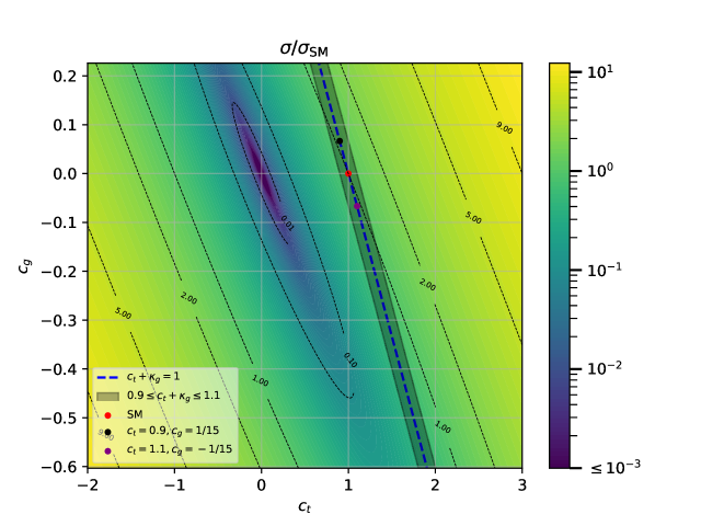
Figure 4: Heat map of the ratio of the HEFT to the SM at the central scale. The colour spectrum is capped at $10^{-3}$. The cut on $p_{T,H}$ is $400~{}\mathrm{G}\mathrm{eV}$.

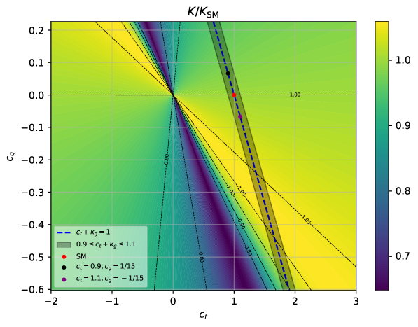
Figure 5: Heat map of the ratio of the NLO K-factors of the HEFT to the SM at the central scale. The cut on $p_{T,H}$ is $400~{}\mathrm{G}\mathrm{eV}$.

$p_{T,H}^{\mathrm{cut}}$	$A$	$B$	$C$	$C_{\mathrm{HTL}}$
0	$15.4\pm 0.2$	$21.3\pm 1.6$	$30.6\pm 2.8$	$30.7\pm 0.2$
50	$9.35\pm 0.13$	$13.4\pm 0.3$	$19.2\pm 0.6$	$18.9\pm 0.4$
100	$2.88\pm 0.04$	$4.16\pm 0.06$	$6.15\pm 0.1$	$6.10\pm 0.09$
200	$(4.57\pm 0.03)\cdot 10^{-1}$	$(7.22\pm 0.09)\cdot 10^{-1}$	$(11.99\pm 0.15)\cdot 10^{-1}$	$(12.1\pm 0.3)\cdot 10^{-1}$
400	$(2.54\pm 0.01)\cdot 10^{-2}$	$(5.61\pm 0.08)\cdot 10^{-2}$	$(13.6\pm 0.1)\cdot 10^{-2}$	$(13.6\pm 0.4)\cdot 10^{-2}$
600	$(2.66\pm 0.01)\cdot 10^{-3}$	$(8.19\pm 0.11)\cdot 10^{-3}$	$(28.3\pm 0.2)\cdot 10^{-3}$	$(28.2\pm 0.3)\cdot 10^{-3}$
800	$(4.14\pm 0.02)\cdot 10^{-4}$	$(16.8\pm 0.2)\cdot 10^{-4}$	$(78.3\pm 0.5)\cdot 10^{-4}$	$(77.7\pm 0.2)\cdot 10^{-4}$

Table 3: Values for $A$,$B$ and $C$ at NLO in $\mathrm{p}\mathrm{b}$ at the central scale. The values for the $p_{T,H}$–cut are given in $\mathrm{G}\mathrm{eV}$. The uncertainties are the uncertainties of the fit.

As can be seen in Fig. 4, the difference to the SM cross section can get very pronounced as we deviate further from the interval $c_{t}+3/2c_{g}\in[0.9,1.1]$. We can also see that the values of $(c_{t},c_{g})=(0.9,1/15)$ and $(c_{t},c_{g})=(1.1,-1/15)$ are at the boundary to where a difference to the SM starts to become significant. We find that $66.67\%$ of the HEFT points with $c_{t}+3/2c_{g}\in[0.9,1.1]$ deviate from the SM result by up to $38\%$. If we enlarge the interval to $[0.8,1.2]$, the deviation for 2/3 of the HEFT points in that interval increases to $41\%$.

In Fig. 5 we show the ratio of the HEFT K-factors to the SM K-factor. We see that the relative K-factors vary significantly as a function of $c_{t}$ and $c_{g}$.

3.2 Higgs boson transverse momentum distributions

The $p_{T,H}$ distribution with a minimum $p_{T}$-cut of $30\,\mathrm{G}\mathrm{eV}$ on the jet is shown in Fig. 6, for the SM, the HTL and two HEFT benchmark points. Up to values of $p_{T,H}\approx 300~{}\mathrm{G}\mathrm{eV}$ there is no significant difference between the considered predictions, but for larger $p_{T,H}$ values the heavy top limit shows large deviations from the SM, whereas the two HEFT parameter points lead to significantly smaller deviations. Thus it is very important to use the SM predictions with full $m_{t}$-dependence, otherwise the approximation given by the HTL could mask enhancements in the tail which are in fact BSM effects.

For the two benchmark points we consider, the BSM effects only lie outside the SM NLO QCD scale uncertainty bands for $p_{T,H}\gtrsim 800~{}\mathrm{G}\mathrm{eV}$. However, the two benchmark points we chose are quite close to the SM. Choosing larger deformations of the SM case would lead to more pronounced effects, visible already at smaller $p_{T,H}$ values. Nonetheless, for very highly boosted Higgs bosons, even small deviations from the SM couplings can lead to characteristic effects. It remains to be investigated whether other SM uncertainties, such as the choice of different top mass renormalisation schemes, can lead to shape distortions that could mask BSM effects. In Ref. Bonciani:2022jmb it was shown that the $p_{T,H}$ distribution with the top quark mass renormalised in the $\overline{\mathrm{MS}}$ scheme falls off faster than in the on-shell (OS) scheme as $p_{T,H}$ increases. However, the ratio OS/$\overline{\mathrm{MS}}$ in the $p_{T,H}$ spectrum stays rather constant for $p_{T,H}$ values between 600  G eV and 1 T eV , while the BSM effects grow much more rapidly with $p_{T,H}$.
Similar considerations hold for the QCD corrections beyond NLO. In Ref. Becker:2020rjp the NLO K-factors have been shown to be rather uniform over the whole $p_{T,H}$ spectrum, both in the full SM as well as for the HTL. For the case of the HTL, the ratio between NNLO and NLO also turned out to be rather flat, NNLO increasing the NLO corrections by about 25% for $400\,\mathrm{G}\mathrm{eV}\leq p_{T,H}\leq 1\,\mathrm{T}\mathrm{eV}$. Thus, a distinctive feature of the anomalous couplings consists in the rapid growth of the shape distortion compared to the SM as $p_{T,H}$ increases.

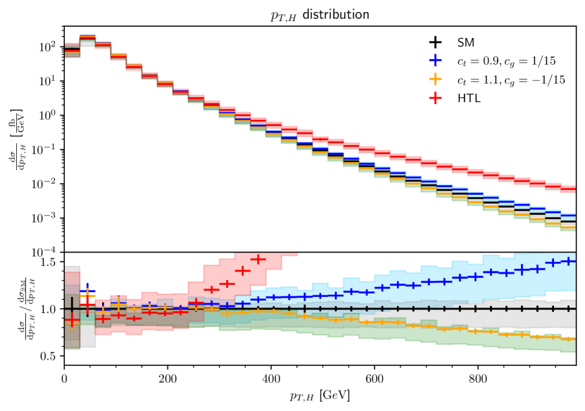
Figure 6: Higgs boson transverse momentum distribution for two HEFT benchmark points, $(c_{t},c_{g})=(0.9,1/15)$ and $(c_{t},c_{g})=(1.1,-1/15)$, compared to the SM case and to the heavy top limit. The bands denote 3-point scale variations around the central scale $\mu_{0}=H_{T}/2$.

4 Conclusions

We have presented results for Higgs boson production in association with one jet, combining full NLO QCD corrections with the leading operators within Higgs Effective Field Theory (HEFT), which can modify the top-Higgs Yukawa coupling and induce an effective Higgs-gluon coupling. We have taken into account constraints arising from the fact that inclusive Higgs production measurements show very good agreement with the SM prediction, assuming that subleading operators, such as the chromomagnetic operator or four-fermion operators, do not play a substantial role. We found that there are combinations of $c_{t}$ and $c_{g}$ that reproduce the inclusive Higgs production cross section at the 10% level, while changing the Higgs + jet cross section to an extent that exceeds the scale uncertainties in the highly boosted Higgs regime, i.e. for $p_{T,H}^{\mathrm{min}}\gtrsim 600~{}\mathrm{G}\mathrm{eV}$. We also found that the NLO K-factor can vary by more than 30% compared to the SM K-factor within the allowed range of $c_{t}$ and $c_{g}$. Furthermore, we showed that including the full top quark mass dependence is important to avoid that the approximation given by the heavy top limit, leading to an enhancement in the tail of the $p_{T,H}$ distribution, is masking a BSM effect.

It remains to be investigated in more detail whether top mass renormalisation scheme uncertainties could swamp the effects of anomalous couplings even for highly boosted Higgs bosons; the results presented in Ref. Bonciani:2022jmb for the SM case suggest that the ratio between on-shell and $\overline{\mathrm{MS}}$ renormalisation schemes for the top quark is rather flat for large $p_{T,H}$ values, while the BSM effects grow rapidly with $p_{T,H}$. Similar considerations hold for QCD corrections beyond NLO, as the K-factors are close to constant in the large $p_{T,H}$ range. This holds for the NLO K-factors both in the HTL and in the full SM, as well as for K_NNLO in the HTL Becker:2020rjp . The effects of subleading operators such as the chromomagnetic or four-fermion operators also deserve further study, as well as electroweak corrections.
We plan to publish the Monte Carlo code underlying our results within the framework of the POWHEG-BOX-V2, after having constructed a grid and an interpolation framework for the virtual 2-loop amplitudes.

A Appendix

In this appendix we list the coefficients $A,B$ and $C$ of the anomalous coupling structures, see Equation 13, for the three scale choices $\mu_{\rm{R}}=\mu_{\rm{F}}=\mu_{0}$, $\mu_{\rm{R}}=\mu_{\rm{F}}=2\mu_{0}$ and $\mu_{\rm{R}}=\mu_{\rm{F}}=\mu_{0}/2$. The uncertainties are the uncertainties from the fit.

$p_{T,H}$ cut [$\mathrm{G}\mathrm{eV}]$	$\mu_{\rm{R}}=\mu_{\rm{F}}=\mu_{0}$	$\mu_{\rm{R}}=\mu_{\rm{F}}=2\mu_{0}$	$\mu_{\rm{R}}=\mu_{\rm{F}}=0.5\mu_{0}$
0	$15.4\pm 0.2$	$12.8\pm 0.2$	$14.4\pm 0.4$
50	$9.35\pm 0.13$	$7.68\pm 0.09$	$9.37\pm 0.24$
100	$2.88\pm 0.04$	$2.36\pm 0.02$	$2.86\pm 0.07$
200	$(4.57\pm 0.03)\cdot 10^{-1}$	$(3.71\pm 0.02)\cdot 10^{-1}$	$(4.70\pm 0.05)\cdot 10^{-1}$
400	$(2.54\pm 0.01)\cdot 10^{-2}$	$(2.01\pm 0.01)\cdot 10^{-2}$	$(2.69\pm 0.02)\cdot 10^{-2}$
600	$(2.66\pm 0.01)\cdot 10^{-3}$	$(2.12\pm 0.01)\cdot 10^{-3}$	$(2.87\pm 0.02)\cdot 10^{-3}$
800	$(4.14\pm 0.02)\cdot 10^{-4}$	$(3.31\pm 0.02)\cdot 10^{-4}$	$(4.50\pm 0.03)\cdot 10^{-4}$

Table 4: Values for A at NLO in $\mathrm{p}\mathrm{b}$

$p_{T,H}$ cut [$\mathrm{G}\mathrm{eV}]$	$\mu_{\rm{R}}=\mu_{\rm{F}}=\mu_{0}$	$\mu_{\rm{R}}=\mu_{\rm{F}}=2\mu_{0}$	$\mu_{\rm{R}}=\mu_{\rm{F}}=0.5\mu_{0}$
0	$21.3\pm 1.6$	$18.3\pm 0.4$	$22.8\pm 1.0$
50	$13.4\pm 0.3$	$11.0\pm 0.2$	$14.8\pm 0.6$
100	$4.16\pm 0.06$	$3.40\pm 0.04$	$4.60\pm 0.11$
200	$(7.22\pm 0.09)\cdot 10^{-1}$	$(5.85\pm 0.06)\cdot 10^{-1}$	$(8.10\pm 0.15)\cdot 10^{-1}$
400	$(5.61\pm 0.08)\cdot 10^{-2}$	$(4.50\pm 0.05)\cdot 10^{-2}$	$(6.43\pm 0.13)\cdot 10^{-2}$
600	$(8.19\pm 0.11)\cdot 10^{-3}$	$(6.56\pm 0.08)\cdot 10^{-3}$	$(9.47\pm 0.18)\cdot 10^{-3}$
800	$(16.8\pm 0.2)\cdot 10^{-4}$	$(13.4\pm 0.2)\cdot 10^{-4}$	$(19.5\pm 0.3)\cdot 10^{-4}$

Table 5: Values for B at NLO in $\mathrm{p}\mathrm{b}$

$p_{T,H}$ cut [$\mathrm{G}\mathrm{eV}]$	$\mu_{\rm{R}}=\mu_{\rm{F}}=\mu_{0}$	$\mu_{\rm{R}}=\mu_{\rm{F}}=2\mu_{0}$	$\mu_{\rm{R}}=\mu_{\rm{F}}=0.5\mu_{0}$
0	$30.6\pm 2.8$	$26.4\pm 0.6$	$37.3\pm 1.6$
50	$19.2\pm 0.6$	$15.8\pm 0.4$	$23.4\pm 1.0$
100	$6.15\pm 0.1$	$5.01\pm 0.07$	$7.48\pm 0.18$
200	$(11.99\pm 0.15)\cdot 10^{-1}$	$(9.76\pm 0.10)\cdot 10^{-1}$	$(14.4\pm 0.3)\cdot 10^{-1}$
400	$(13.6\pm 0.1)\cdot 10^{-2}$	$(11.2\pm 0.1)\cdot 10^{-2}$	$(16.4\pm 0.2)\cdot 10^{-2}$
600	$(28.3\pm 0.2)\cdot 10^{-3}$	$(23.0\pm 0.1)\cdot 10^{-3}$	$(34.2\pm 0.3)\cdot 10^{-3}$
800	$(78.3\pm 0.5)\cdot 10^{-4}$	$(63.2\pm 0.3)\cdot 10^{-4}$	$(95.0\pm 0.7)\cdot 10^{-4}$

Table 6: Values for C at NLO in $\mathrm{p}\mathrm{b}$

References

- (1) R. V. Harlander and T. Neumann, Probing the nature of the Higgs-gluon coupling, Phys. Rev. D 88 (2013) 074015, [arXiv:1308.2225].
- (2) A. Azatov and A. Paul, Probing Higgs couplings with high Higgs production, JHEP 01 (2014) 014, [arXiv:1309.5273].
- (3) A. Banfi, A. Martin, and V. Sanz, Probing top-partners in Higgs+jets, JHEP 08 (2014) 053, [arXiv:1308.4771].
- (4) C. Grojean, E. Salvioni, M. Schlaffer, and A. Weiler, Very boosted Higgs in gluon fusion, JHEP 05 (2014) 022, [arXiv:1312.3317].
- (5) M. Schlaffer, M. Spannowsky, M. Takeuchi, A. Weiler, and C. Wymant, Boosted Higgs Shapes, Eur. Phys. J. C 74 (2014), no. 10 3120, [arXiv:1405.4295].
- (6) S. Dawson, I. M. Lewis, and M. Zeng, Effective field theory for Higgs boson plus jet production, Phys. Rev. D 90 (2014), no. 9 093007, [arXiv:1409.6299].
- (7) M. Buschmann, D. Goncalves, S. Kuttimalai, M. Schonherr, F. Krauss, and T. Plehn, Mass Effects in the Higgs-Gluon Coupling: Boosted vs Off-Shell Production, JHEP 02 (2015) 038, [arXiv:1410.5806].
- (8) U. Langenegger, M. Spira, and I. Strebel, Testing the Higgs Boson Coupling to Gluons, arXiv:1507.01373.
- (9) A. Azatov, C. Grojean, A. Paul, and E. Salvioni, Resolving gluon fusion loops at current and future hadron colliders, JHEP 09 (2016) 123, [arXiv:1608.00977].
- (10) J. M. Lindert, K. Kudashkin, K. Melnikov, and C. Wever, Higgs bosons with large transverse momentum at the LHC, Phys. Lett. B 782 (2018) 210–214, [arXiv:1801.08226].
- (11) J. Alison et al., Higgs boson potential at colliders: Status and perspectives, Rev. Phys. 5 (2020) 100045, [arXiv:1910.00012].
- (12) F. Maltoni, E. Vryonidou, and C. Zhang, Higgs production in association with a top-antitop pair in the Standard Model Effective Field Theory at NLO in QCD, JHEP 10 (2016) 123, [arXiv:1607.05330].
- (13) M. Grazzini, A. Ilnicka, M. Spira, and M. Wiesemann, Modeling BSM effects on the Higgs transverse-momentum spectrum in an EFT approach, JHEP 03 (2017) 115, [arXiv:1612.00283].
- (14) M. Grazzini, A. Ilnicka, and M. Spira, Higgs boson production at large transverse momentum within the SMEFT: analytical results, Eur. Phys. J. C 78 (2018), no. 10 808, [arXiv:1806.08832].
- (15) M. Battaglia, M. Grazzini, M. Spira, and M. Wiesemann, Sensitivity to BSM effects in the Higgs pT spectrum within SMEFT, JHEP 11 (2021) 173, [arXiv:2109.02987].
- (16) F. Maltoni, G. Ventura, and E. Vryonidou, Impact of SMEFT renormalisation group running on Higgs production at the LHC, arXiv:2406.06670.
- (17) U. Baur and E. W. N. Glover, Higgs Boson Production at Large Transverse Momentum in Hadronic Collisions, Nucl. Phys. B 339 (1990) 38–66.
- (18) K. Melnikov, L. Tancredi, and C. Wever, Two-loop amplitude mediated by a nearly massless quark, JHEP 11 (2016) 104, [arXiv:1610.03747].
- (19) S. P. Jones, M. Kerner, and G. Luisoni, Next-to-Leading-Order QCD Corrections to Higgs Boson Plus Jet Production with Full Top-Quark Mass Dependence, Phys. Rev. Lett. 120 (2018), no. 16 162001, [arXiv:1802.00349]. [Erratum: Phys.Rev.Lett. 128, 059901 (2022)].
- (20) K. Becker et al., Precise predictions for boosted Higgs production, SciPost Phys. Core 7 (2024) 001, [arXiv:2005.07762].
- (21) T. Neumann, NLO Higgs+jet production at large transverse momenta including top quark mass effects, J. Phys. Comm. 2 (2018), no. 9 095017, [arXiv:1802.02981].
- (22) X. Chen, A. Huss, S. P. Jones, M. Kerner, J. N. Lang, J. M. Lindert, and H. Zhang, Top-quark mass effects in H+jet and H+2 jets production, JHEP 03 (2022) 096, [arXiv:2110.06953].
- (23) R. Bonciani, V. Del Duca, H. Frellesvig, J. M. Henn, F. Moriello, and V. A. Smirnov, Two-loop planar master integrals for Higgs partons with full heavy-quark mass dependence, JHEP 12 (2016) 096, [arXiv:1609.06685].
- (24) R. Bonciani, V. Del Duca, H. Frellesvig, J. M. Henn, M. Hidding, L. Maestri, F. Moriello, G. Salvatori, and V. A. Smirnov, Evaluating a family of two-loop non-planar master integrals for Higgs + jet production with full heavy-quark mass dependence, JHEP 01 (2020) 132, [arXiv:1907.13156].
- (25) H. Frellesvig, M. Hidding, L. Maestri, F. Moriello, and G. Salvatori, The complete set of two-loop master integrals for Higgs + jet production in QCD, JHEP 06 (2020) 093, [arXiv:1911.06308].
- (26) R. Bonciani, V. Del Duca, H. Frellesvig, M. Hidding, V. Hirschi, F. Moriello, G. Salvatori, G. Somogyi, and F. Tramontano, Next-to-leading-order QCD corrections to Higgs production in association with a jet, Phys. Lett. B 843 (2023) 137995, [arXiv:2206.10490].
- (27) P. Pietrulewicz and M. Stahlhofen, Two-loop bottom mass effects on the Higgs transverse momentum spectrum in top-induced gluon fusion, JHEP 05 (2023) 175, [arXiv:2302.06623].
- (28) M. Bonetti, E. Panzer, V. A. Smirnov, and L. Tancredi, Two-loop mixed QCD-EW corrections to , JHEP 11 (2020) 045, [arXiv:2007.09813].
- (29) M. Becchetti, F. Moriello, and A. Schweitzer, Two-loop amplitude for mixed QCD-EW corrections to , JHEP 04 (2022) 139, [arXiv:2112.07578].
- (30) M. Bonetti, E. Panzer, and L. Tancredi, Two-loop mixed QCD-EW corrections to , and , JHEP 06 (2022) 115, [arXiv:2203.17202].
- (31) M. Becchetti, R. Bonciani, V. Casconi, V. Del Duca, and F. Moriello, Planar master integrals for the two-loop light-fermion electroweak corrections to Higgs plus jet production, JHEP 12 (2018) 019, [arXiv:1810.05138].
- (32) J. Davies, K. Schönwald, M. Steinhauser, and H. Zhang, Next-to-leading order electroweak corrections to and in the large- limit, JHEP 10 (2023) 033, [arXiv:2308.01355].
- (33) U. Haisch and M. Niggetiedt, Exact two-loop amplitudes for Higgs plus jet production with a cubic Higgs self-coupling, arXiv:2408.13186.
- (34) R. Boughezal, F. Caola, K. Melnikov, F. Petriello, and M. Schulze, Higgs boson production in association with a jet at next-to-next-to-leading order, Phys. Rev. Lett. 115 (2015), no. 8 082003, [arXiv:1504.07922].
- (35) R. Boughezal, C. Focke, W. Giele, X. Liu, and F. Petriello, Higgs boson production in association with a jet at NNLO using jettiness subtraction, Phys. Lett. B748 (2015) 5–8, [arXiv:1505.03893].
- (36) F. Caola, K. Melnikov, and M. Schulze, Fiducial cross sections for Higgs boson production in association with a jet at next-to-next-to-leading order in QCD, Phys. Rev. D 92 (2015), no. 7 074032, [arXiv:1508.02684].
- (37) X. Chen, J. Cruz-Martinez, T. Gehrmann, E. W. N. Glover, and M. Jaquier, NNLO QCD corrections to Higgs boson production at large transverse momentum, JHEP 10 (2016) 066, [arXiv:1607.08817].
- (38) J. M. Campbell, R. K. Ellis, and S. Seth, H + 1 jet production revisited, JHEP 10 (2019) 136, [arXiv:1906.01020].
- (39) X. Chen, T. Gehrmann, E. W. N. Glover, and A. Huss, Fiducial cross sections for the four-lepton decay mode in Higgs-plus-jet production up to NNLO QCD, JHEP 07 (2019) 052, [arXiv:1905.13738].
- (40) X. Chen, T. Gehrmann, E. W. N. Glover, and A. Huss, Fiducial cross sections for the lepton-pair-plus-photon decay mode in Higgs production up to NNLO QCD, JHEP 01 (2022) 053, [arXiv:2111.02157].
- (41) J. R. Andersen, B. Ducloué, C. Elrick, H. Hassan, A. Maier, G. Nail, J. Paltrinieri, A. Papaefstathiou, and J. M. Smillie, HEJ 2.2: W boson pairs and Higgs boson plus jet production at high energies, arXiv:2303.15778.
- (42) J. R. Andersen, H. Hassan, A. Maier, J. Paltrinieri, A. Papaefstathiou, and J. M. Smillie, High energy resummed predictions for the production of a Higgs boson with at least one jet, JHEP 03 (2023) 001, [arXiv:2210.10671].
- (43) T. Liu, A. A. Penin, and A. Rehman, Light quark mediated Higgs boson production in association with a jet at the next-to-next-to-leading order and beyond, JHEP 04 (2024) 031, [arXiv:2402.18625].
- (44) ATLAS Collaboration, G. Aad et al., Identification of boosted Higgs bosons decaying into -quark pairs with the ATLAS detector at 13 TeV, Eur. Phys. J. C 79 (2019), no. 10 836, [arXiv:1906.11005].
- (45) ATLAS Collaboration, G. Aad et al., Constraints on Higgs boson production with large transverse momentum using decays in the ATLAS detector, Phys. Rev. D 105 (2022), no. 9 092003, [arXiv:2111.08340].
- (46) CMS Collaboration, A. M. Sirunyan et al., Inclusive search for highly boosted Higgs bosons decaying to bottom quark-antiquark pairs in proton-proton collisions at 13 TeV, JHEP 12 (2020) 085, [arXiv:2006.13251].
- (47) CMS Collaboration, A. Hayrapetyan et al., Measurement of the Production Cross Section of a Higgs Boson with Large Transverse Momentum in Its Decays to a Pair of Leptons in Proton-Proton Collisions at = 13 TeV, arXiv:2403.20201.
- (48) F. Feruglio, The Chiral approach to the electroweak interactions, Int. J. Mod. Phys. A 8 (1993) 4937–4972, [hep-ph/9301281].
- (49) C. P. Burgess, J. Matias, and M. Pospelov, A Higgs or not a Higgs? What to do if you discover a new scalar particle, Int. J. Mod. Phys. A 17 (2002) 1841–1918, [hep-ph/9912459].
- (50) B. Grinstein and M. Trott, A Higgs-Higgs bound state due to new physics at a TeV, Phys. Rev. D 76 (2007) 073002, [arXiv:0704.1505].
- (51) R. Contino, C. Grojean, M. Moretti, F. Piccinini, and R. Rattazzi, Strong Double Higgs Production at the LHC, JHEP 05 (2010) 089, [arXiv:1002.1011].
- (52) R. Alonso, M. B. Gavela, L. Merlo, S. Rigolin, and J. Yepes, The Effective Chiral Lagrangian for a Light Dynamical ”Higgs Particle”, Phys. Lett. B 722 (2013) 330–335, [arXiv:1212.3305]. [Erratum: Phys.Lett.B 726, 926 (2013)].
- (53) G. Buchalla, O. Catà, and C. Krause, Complete Electroweak Chiral Lagrangian with a Light Higgs at NLO, Nucl. Phys. B 880 (2014) 552–573, [arXiv:1307.5017]. [Erratum: Nucl.Phys.B 913, 475–478 (2016)].
- (54) N. P. Hartland, F. Maltoni, E. R. Nocera, J. Rojo, E. Slade, E. Vryonidou, and C. Zhang, A Monte Carlo global analysis of the Standard Model Effective Field Theory: the top quark sector, JHEP 04 (2019) 100, [arXiv:1901.05965].
- (55) E. Celada, T. Giani, J. ter Hoeve, L. Mantani, J. Rojo, A. N. Rossia, M. O. A. Thomas, and E. Vryonidou, Mapping the SMEFT at High-Energy Colliders: from LEP and the (HL-)LHC to the FCC-ee, arXiv:2404.12809.
- (56) W. Buchmuller and D. Wyler, Effective Lagrangian Analysis of New Interactions and Flavor Conservation, Nucl. Phys. B 268 (1986) 621–653.
- (57) B. Grzadkowski, M. Iskrzynski, M. Misiak, and J. Rosiek, Dimension-Six Terms in the Standard Model Lagrangian, JHEP 10 (2010) 085, [arXiv:1008.4884].
- (58) I. Brivio and M. Trott, The Standard Model as an Effective Field Theory, Phys. Rept. 793 (2019) 1–98, [arXiv:1706.08945].
- (59) G. Isidori, F. Wilsch, and D. Wyler, The standard model effective field theory at work, Rev. Mod. Phys. 96 (2024), no. 1 015006, [arXiv:2303.16922].
- (60) C. Arzt, M. B. Einhorn, and J. Wudka, Patterns of deviation from the standard model, Nucl. Phys. B 433 (1995) 41–66, [hep-ph/9405214].
- (61) G. Buchalla, G. Heinrich, C. Müller-Salditt, and F. Pandler, Loop counting matters in SMEFT, SciPost Phys. 15 (2023), no. 3 088, [arXiv:2204.11808].
- (62) A. Banfi, B. M. Dillon, W. Ketaiam, and S. Kvedaraite, Composite Higgs at high transverse momentum, JHEP 01 (2020) 089, [arXiv:1905.12747].
- (63) J. R. Ellis, M. K. Gaillard, and D. V. Nanopoulos, A Phenomenological Profile of the Higgs Boson, Nucl. Phys. B 106 (1976) 292.
- (64) A. I. Vainshtein, V. I. Zakharov, and M. A. Shifman, Higgs Particles, Sov. Phys. Usp. 23 (1980) 429–449.
- (65) S. Dawson and H. E. Haber, Higgs Boson Low-energy Theorems and Their Applications, Int. J. Mod. Phys. A 7 (1992) 107–120.
- (66) ATLAS Collaboration, G. Aad et al., Study of High-Transverse-Momentum Higgs Boson Production in Association with a Vector Boson in the qqbb Final State with the ATLAS Detector, Phys. Rev. Lett. 132 (2024), no. 13 131802, [arXiv:2312.07605].
- (67) GoSam Collaboration, G. Cullen, N. Greiner, G. Heinrich, G. Luisoni, P. Mastrolia, G. Ossola, T. Reiter, and F. Tramontano, Automated One-Loop Calculations with GoSam, Eur. Phys. J. C 72 (2012) 1889, [arXiv:1111.2034].
- (68) GoSam Collaboration, G. Cullen et al., GS-2.0: a tool for automated one-loop calculations within the Standard Model and beyond, Eur. Phys. J. C 74 (2014), no. 8 3001, [arXiv:1404.7096].
- (69) C. Degrande, C. Duhr, B. Fuks, D. Grellscheid, O. Mattelaer, and T. Reiter, UFO - The Universal FeynRules Output, Comput. Phys. Commun. 183 (2012) 1201–1214, [arXiv:1108.2040].
- (70) L. Darmé et al., UFO 2.0: the ‘Universal Feynman Output’ format, Eur. Phys. J. C 83 (2023), no. 7 631, [arXiv:2304.09883].
- (71) G. Buchalla, M. Capozi, A. Celis, G. Heinrich, and L. Scyboz, Higgs boson pair production in non-linear Effective Field Theory with full -dependence at NLO QCD, JHEP 09 (2018) 057, [arXiv:1806.05162].
- (72) G. Luisoni, P. Nason, C. Oleari, and F. Tramontano, /HZ + 0 and 1 jet at NLO with the POWHEG BOX interfaced to GoSam and their merging within MiNLO, JHEP 10 (2013) 083, [arXiv:1306.2542].
- (73) P. Nason, A New method for combining NLO QCD with shower Monte Carlo algorithms, JHEP 11 (2004) 040, [hep-ph/0409146].
- (74) S. Frixione, P. Nason, and C. Oleari, Matching NLO QCD computations with Parton Shower simulations: the POWHEG method, JHEP 11 (2007) 070, [arXiv:0709.2092].
- (75) S. Alioli, P. Nason, C. Oleari, and E. Re, A general framework for implementing NLO calculations in shower Monte Carlo programs: the POWHEG BOX, JHEP 06 (2010) 043, [arXiv:1002.2581].
- (76) P. Nogueira, Automatic Feynman Graph Generation, J. Comput. Phys. 105 (1993) 279–289.
- (77) J. Kuipers, T. Ueda, J. A. M. Vermaseren, and J. Vollinga, FORM version 4.0, Comput. Phys. Commun. 184 (2013) 1453–1467, [arXiv:1203.6543].
- (78) G. Cullen, M. Koch-Janusz, and T. Reiter, Spinney: A Form Library for Helicity Spinors, Comput. Phys. Commun. 182 (2011) 2368–2387, [arXiv:1008.0803].
- (79) P. Mastrolia, G. Ossola, T. Reiter, and F. Tramontano, Scattering AMplitudes from Unitarity-based Reduction Algorithm at the Integrand-level, JHEP 08 (2010) 080, [arXiv:1006.0710].
- (80) H. van Deurzen, Associated Higgs Production at NLO with GoSam, Acta Phys. Polon. B 44 (2013), no. 11 2223–2230.
- (81) T. Binoth, J. P. Guillet, G. Heinrich, E. Pilon, and T. Reiter, Golem95: A Numerical program to calculate one-loop tensor integrals with up to six external legs, Comput. Phys. Commun. 180 (2009) 2317–2330, [arXiv:0810.0992].
- (82) G. Cullen, J. P. Guillet, G. Heinrich, T. Kleinschmidt, E. Pilon, T. Reiter, and M. Rodgers, Golem95C: A library for one-loop integrals with complex masses, Comput. Phys. Commun. 182 (2011) 2276–2284, [arXiv:1101.5595].
- (83) J. P. Guillet, G. Heinrich, and J. F. von Soden-Fraunhofen, Tools for NLO automation: extension of the golem95C integral library, Comput. Phys. Commun. 185 (2014) 1828–1834, [arXiv:1312.3887].
- (84) T. Peraro, Ninja: Automated Integrand Reduction via Laurent Expansion for One-Loop Amplitudes, Comput. Phys. Commun. 185 (2014) 2771–2797, [arXiv:1403.1229].
- (85) A. van Hameren, OneLOop: For the evaluation of one-loop scalar functions, Comput. Phys. Commun. 182 (2011) 2427–2438, [arXiv:1007.4716].
- (86) R. K. Ellis and G. Zanderighi, Scalar one-loop integrals for QCD, JHEP 02 (2008) 002, [arXiv:0712.1851].
- (87) A. von Manteuffel and C. Studerus, Reduze 2 - Distributed Feynman Integral Reduction, arXiv:1201.4330.
- (88) S. Borowka, G. Heinrich, S. P. Jones, M. Kerner, J. Schlenk, and T. Zirke, SecDec-3.0: numerical evaluation of multi-scale integrals beyond one loop, Comput. Phys. Commun. 196 (2015) 470–491, [arXiv:1502.06595].
- (89) S. Borowka, G. Heinrich, S. Jahn, S. P. Jones, M. Kerner, J. Schlenk, and T. Zirke, pySecDec: a toolbox for the numerical evaluation of multi-scale integrals, Comput. Phys. Commun. 222 (2018) 313–326, [arXiv:1703.09692].
- (90) G. Heinrich, S. Jahn, S. P. Jones, M. Kerner, F. Langer, V. Magerya, A. Pöldaru, J. Schlenk, and E. Villa, Expansion by regions with pySecDec, Comput. Phys. Commun. 273 (2022) 108267, [arXiv:2108.10807].
- (91) G. Heinrich, S. P. Jones, M. Kerner, V. Magerya, A. Olsson, and J. Schlenk, Numerical scattering amplitudes with pySecDec, Comput. Phys. Commun. 295 (2024) 108956, [arXiv:2305.19768].
- (92) M. Boggia et al., The HiggsTools handbook: a beginners guide to decoding the Higgs sector, J. Phys. G 45 (2018), no. 6 065004, [arXiv:1711.09875].
- (93) T. Gehrmann, M. Jaquier, E. W. N. Glover, and A. Koukoutsakis, Two-Loop QCD Corrections to the Helicity Amplitudes for 3 partons, JHEP 02 (2012) 056, [arXiv:1112.3554].
- (94) M. Spira, A. Djouadi, D. Graudenz, and P. M. Zerwas, Higgs boson production at the LHC, Nucl. Phys. B 453 (1995) 17–82, [hep-ph/9504378].
- (95) J. Butterworth et al., PDF4LHC recommendations for LHC Run II, J. Phys. G 43 (2016) 023001, [arXiv:1510.03865].
- (96) S. Dulat, T.-J. Hou, J. Gao, M. Guzzi, J. Huston, P. Nadolsky, J. Pumplin, C. Schmidt, D. Stump, and C. P. Yuan, New parton distribution functions from a global analysis of quantum chromodynamics, Phys. Rev. D 93 (2016), no. 3 033006, [arXiv:1506.07443].
- (97) L. A. Harland-Lang, A. D. Martin, P. Motylinski, and R. S. Thorne, Parton distributions in the LHC era: MMHT 2014 PDFs, Eur. Phys. J. C 75 (2015), no. 5 204, [arXiv:1412.3989].
- (98) NNPDF Collaboration, R. D. Ball et al., Parton distributions for the LHC Run II, JHEP 04 (2015) 040, [arXiv:1410.8849].
- (99) A. Buckley, J. Ferrando, S. Lloyd, K. Nordström, B. Page, M. Rüfenacht, M. Schönherr, and G. Watt, LHAPDF6: parton density access in the LHC precision era, Eur. Phys. J. C 75 (2015) 132, [arXiv:1412.7420].
- (100) M. Cacciari, G. P. Salam, and G. Soyez, The anti- jet clustering algorithm, JHEP 04 (2008) 063, [arXiv:0802.1189].
- (101) M. Cacciari and G. P. Salam, Dispelling the myth for the jet-finder, Phys. Lett. B 641 (2006) 57–61, [hep-ph/0512210].
- (102) M. Cacciari, G. P. Salam, and G. Soyez, FastJet User Manual, Eur. Phys. J. C 72 (2012) 1896, [arXiv:1111.6097].
- (103) SMEFiT Collaboration, J. J. Ethier, G. Magni, F. Maltoni, L. Mantani, E. R. Nocera, J. Rojo, E. Slade, E. Vryonidou, and C. Zhang, Combined SMEFT interpretation of Higgs, diboson, and top quark data from the LHC, JHEP 11 (2021) 089, [arXiv:2105.00006].
- (104) F. Caola, S. Forte, S. Marzani, C. Muselli, and G. Vita, The Higgs transverse momentum spectrum with finite quark masses beyond leading order, JHEP 08 (2016) 150, [arXiv:1606.04100].