Distributionally Robust Stochastic Data-Driven Predictive Control
with Optimized Feedback Gain

Abstract

We consider the problem of direct data-driven predictive control for unknown stochastic linear time-invariant (LTI) systems with partial state observation. Building upon our previous research on data-driven stochastic control, this paper (i) relaxes the assumption of Gaussian process and measurement noise, and (ii) enables optimization of the gain matrix within the affine feedback policy. Output safety constraints are modelled using conditional value-at-risk, and enforced in a distributionally robust sense. Under idealized assumptions, we prove that our proposed data-driven control method yields control inputs identical to those produced by an equivalent model-based stochastic predictive controller. A simulation study illustrates the enhanced performance of our approach over previous designs.

I Introduction

Model predictive control (MPC) is a widely used technique for multivariate control [1], adept at handling constraints on inputs, states and outputs while optimizing complex performance objectives. Constraints typically model actuator limits, or encode safety constraints in safety-critical applications, and MPC employs a system model to predict how inputs influence state evolution. Both deterministic and stochastic frameworks have been developed to account for plant uncertainty in MPC. While Robust MPC [2] approaches model uncertainty in a worst-case deterministic sense, work on Stochastic MPC (SMPC) [3] has focused on describing model uncertainty probabilistically. SMPC methods optimize over feedback control policies rather than control actions, resulting in performance benefits when compared to the naïve use of deterministic MPC [4], and accommodate probabilistic and risk-aware constraints.

The system model required by MPC (and SMPC) is sometimes obtained from identification, making MPC an indirect design method, since one goes from data to a controller through an intermediate modelling step [5]. In contrast, data-driven or direct methods seek to compute controllers directly from input-output data, showing promise for complex or difficult-to-model systems [6]. Accounting for constraints in control, Data-Driven Predictive Control (DDPC) methods were developed, including Data-Enabled Predictive Control (DeePC) [7, 8, 9] and Subspace Predictive Control (SPC) [10], both of which have been applied in multiple experiments [11, 12, 13]. For deterministic LTI systems in theory, both DeePC and SPC produce equivalent control actions as from MPC.

Real-world systems often deviate from idealized deterministic LTI models, exhibiting stochastic and non-linear behavior, with noise-corrupted data. To address these challenges, data-driven methods must account for noisy data and measurements. For instance, in SPC applications, required predictor matrices are often computed using denoising techniques [10]. Regularized and distributionally robust DeePC were also developed for stochastic systems [7, 8, 9]. Unlike in the deterministic case, however, these stochastic adaptations of DeePC and SPC lack theoretical equivalence to model-based MPC.

Recognizing this gap, some recent advancements in DDPC have aimed to establish equivalence with MPC methods for stochastic systems. The work in [14, 15] proposed a DDPC framework for stochastic systems, and their method performs equivalently to SMPC if stochastic signals can be exactly expressed by their Polynomial Chaos Expansion. This paper builds in particular on our previous work [16], where we proposed a data-driven control method for stochastic systems, without estimation of disturbance as required in [15, 14], and established that the method has equivalent control performance to SMPC when offline data is noise-free.

Contribution: This paper contributes towards the continued development of high-performance DDPC methods for stochastic systems. Specifically, in this paper we develop a stochastic DDPC strategy utilizing distributionally robust conditional value-at-risk constraints, providing an improved safety constraint description when compared to our prior work in [16], and providing robustness against non-Gaussian (i.e., possibly heavy-tailed) process and measurement noise. Additionally, in contrast with the fixed feedback gain in [16], we consider control policies where feedback gains are decision variables in the optimization, giving a more flexible parameterization of control policies. As theoretical support for the approach, under technical conditions, we establish equivalence between our proposed design and a corresponding SMPC. Finally, a simulation case study compares and contrasts our design with other recent stochastic and data-driven control strategies.

Notation: Let $M^{\dagger}$ be the pseudo-inverse of a matrix $M$. Let $\otimes$ denote the Kronecker product. Let $\mathbb{S}^{q}_{+}$ (resp. $\mathbb{S}^{q}_{++}$) be the set of $q\times q$ positive semi-definite (resp. definite) matrices. Let $\mathrm{col}(M_{1},\ldots,M_{k})$ (resp. $\mathrm{Diag}(M_{1},\ldots,M_{k})$) denote the vertical (resp. diagonal) concatenation of matrices / vectors $M_{1},\ldots,M_{k}$. Let $\mathbb{Z}_{[a,b]}:=[a,b]\cap\mathbb{Z}$ denote a set of consecutive integers from $a$ to $b$, and let $\mathbb{Z}_{[a,b)}:=\mathbb{Z}_{[a,b-1]}$. For a ^q-valued discrete-time signal $z_{t}$ with integer index $t$, let $z_{[t_{1},t_{2}]}$ denote either a sequence $\{z_{t}\}_{t=t_{1}}^{t_{2}}$ or a concatenated vector $\mathrm{col}(z_{t_{1}},\ldots,z_{t_{2}})\in{}^{q(t_{2}-t_{1}+1)}$ where the usage is clear from the context; similarly, let $z_{[t_{1},t_{2})}:=z_{[t_{1},t_{2}-1]}$. A matrix sequence $\{M_{t}\}_{t=t_{1}}^{t_{2}}$ and a function sequence $\{\pi_{t}(\cdot)\}_{t=t_{1}}^{t_{2}}$ are denoted by $M_{[t_{1},t_{2}]}$ and $\pi_{[t_{1},t_{2}]}$ respectively.

II Problem Setup

Consider a stochastic linear time-invariant (LTI) system

$$x_{t+1}=Ax_{t}+Bu_{t}+w_{t},\quad y_{t}=Cx_{t}+Du_{t}+v_{t}$$ (1)

with input $u_{t}\in{}^{m}$, state $x_{t}\in{}^{n}$, output $y_{t}\in{}^{p}$, process noise $w_{t}\in{}^{n}$, and measurement noise $v_{t}\in{}^{p}$. The system $(A,B,C,D)$ is assumed as a minimal realization, but the matrices themselves are unknown and the state $x_{t}$ is unmeasured; we have access only to the input $u_{t}$ and output $y_{t}$ in (1). The probability distributions of $w_{t}$ and $v_{t}$ are unknown, but we assume that $w_{t}$ and $v_{t}$ have zero mean and zero auto-correlation (white noise), are uncorrelated, and their variances $\Sigma^{\sf w}\in\mathbb{S}^{n}_{+}$ and $\Sigma^{\sf v}\in\mathbb{S}^{p}_{++}$ are known. The initial state $x_{0}$ has given mean $\mu^{\sf x}_{\sf ini}$ and variance $\Sigma^{\sf x}$ and is uncorrelated with the noise. We record these conditions as

$$\mathbb{E}\big{[}\text{\small$\begin{bmatrix}w_{t}\\[-2.25pt] v_{t}\end{bmatrix}$}\big{]}=0,\quad\mathbb{E}\big{[}\text{\small$\begin{bmatrix}w_{t}\\[-2.25pt] v_{t}\end{bmatrix}$}\text{\small$\begin{bmatrix}w_{s}\\[-2.25pt] v_{s}\end{bmatrix}$}\!\raisebox{2.5pt}{${}^{\sf T}$}\big{]}=\text{\small$\begin{bmatrix}\delta_{ts}\Sigma^{\sf w}&0\\[-2.25pt] 0&\delta_{ts}\Sigma^{\sf v}\end{bmatrix}$},$$ (2)

$$\mathbb{E}[x_{0}]=\mu^{\sf x}_{\sf ini},\quad\mathrm{Var}[x_{0}]=\Sigma^{\sf x},\quad\mathbb{E}\big{[}x_{0}\text{\small$\begin{bmatrix}w_{t}\\[-2.25pt] v_{t}\end{bmatrix}$}\!\raisebox{2.5pt}{${}^{\sf T}$}\big{]}=0,$$ (3)

with $\delta_{ts}$ the Kronecker delta. Assume $(A,\Sigma^{\sf w})$ is stabilizable.

In a reference tracking control problem for (1), the objective is for the output $y_{t}$ to follow a specified reference signal $r_{t}\in{}^{p}$. The trade-off between tracking error and control effort may be encoded in an instantaneous cost

$$J_{t}(u_{t},y_{t}):=\|y_{t}-r_{t}\|_{Q}^{2}+\|u_{t}\|_{R}^{2}$$ (4)

to be minimized over a time horizon, with user-selected parameters $Q\in\mathbb{S}^{p}_{+}$ and $R\in\mathbb{S}^{m}_{++}$. This tracking should be achieved subject to constraints on the inputs and outputs. We consider here polytopic constraints, which in a deterministic setting would take the form $E\text{\small$\begin{bmatrix}u_{t}\\[-2.25pt] y_{t}\end{bmatrix}$}\leq f$ for all $t\in\mathbb{N}_{\geq 0}$, and for some fixed matrix $E\in{}^{q\times(m+p)}$ and vector $f\in{}^{q}$. We can equivalently express these constraints as the single constraint $h(u_{t},y_{t})\leq 0$, where

$$h(u_{t},y_{t}):={\max}_{\,i\in\{1,\ldots,q\}}\;e^{\sf T}_{i}\text{\small$\begin{bmatrix}u_{t}\\[-2.25pt] y_{t}\end{bmatrix}$}-f_{i},$$ (5)

with $e_{i}\in{}^{m+p}$ the transposed $i$-th row of $E$ and $f_{i}\in\real$ the $i$-th entry of $f$. For the system (1) which is subject to (possibly unbounded) stochastic disturbances, the deterministic constraint $h(u_{t},y_{t})\leq 0$ must be relaxed. Beyond a traditional chance constraint $\mathbb{P}[h(u_{t},y_{t})\leq 0]\geq 1-\alpha$ with a violation probability $\alpha\in(0,1)$, a conditional value-at-risk (CVaR) constraint is more conservative; the CVaR at level $\alpha$ of $h(u_{t},y_{t})$ is defined as the expected value of $h(u_{t},y_{t})$ in the $\alpha\cdot$ 100% worst cases, and takes extreme violations into account. With the noise distributions unknown, we must further guarantee satisfaction of the CVaR constraint for all possible distributions under consideration. Let $\mathbb{D}$ denote a joint distribution of all random variables in (1) satisfying (2) and (3), and let the ambiguity set $\mathcal{D}$ be the set of all such distributions. The distributionally robust CVaR (DR-CVaR) constraint [17, 18] is then

$${\sup}_{\,\mathbb{D}\in\mathcal{D}}\;\mathbb{D}\text{-}\mathrm{CVaR}_{\alpha}[h(u_{t},y_{t})]\leq 0,$$ (6)

where $\mathbb{D}\text{-}\mathrm{CVaR}_{\alpha}[z]$ is the CVaR value of a random variable $z\in\real$ at level $\alpha$ given distribution $\mathbb{D}$.

If the system matrices $A,B,C,D$ were known, this constrained tracking control problem subject to (6) can be approached using SMPC, as described in Section III-A. Our objective is to develop a data-driven control method that produces equivalent control inputs as produced by SMPC.

III Stochastic Model-Based and Data-Driven Predictive Control

We introduce a model-based SMPC framework in Section III-A and propose a data-driven control method in Section III-B, with their theoretical equivalence in Section III-C.

III-A A framework of Stochastic Model Predictive Control

We focus here on output-feedback SMPC [19, 20, 21] which typically combines state estimation and feedback control. The formulation here broadly follows our prior work [16], but we now consider a DR-CVaR constraint in place of chance constraints, and we will allow optimization over the feedback gain. This SMPC scheme merges the established works on DR constrained control [17, 18] and output-error feedback [22], while the combined framework is part of our contribution.

III-A1 State Estimation

SMPC follows a receding-horizon strategy and makes decisions for $N$ upcoming steps at each control step. At control step $t=k$, we begin with prior information of the mean and variance of state $x_{k}$, namely

$$\mathbb{E}[x_{k}]=\mu^{\sf x}_{k},\qquad\mathrm{Var}[x_{k}]=\Sigma^{\sf x},$$ (7)

where the mean $\mu^{\sf x}_{k}$ is computed from a state estimator to be described next; at the initial step $k=0$, $\mu^{\sf x}_{0}=\mu^{\sf x}_{\sf ini}$ is a given parameter as in (3). For simplicity of computation, we let $\Sigma^{\sf x}$ in (3) and (7) be the steady-state variance through the Kalman filter, as the unique positive semi-definite solution to the associated discrete-time algebraic Riccatti equation (DARE) (8a), with observer gain $L_{\sf L}\in{}^{n\times p}$ in (8b).

$$\Sigma^{\sf x}=(A-L_{\sf L}C)\Sigma^{\sf x}A^{\sf T}+\Sigma^{\sf w}$$ (8a)

$$L_{\sf L}:=A\Sigma^{\sf x}C^{\sf T}(C\Sigma^{\sf x}C^{\sf T}+\Sigma^{\sf v})^{-1}$$ (8b)

Estimates $\hat{x}_{t}$ of future states over the desired horizon are computed through the observer, with innovation $\nu_{t}\in{}^{p}$,

$$\nu_{t} :=y_{t}-C\hat{x}_{t}-Du_{t}, t\in\mathbb{Z}_{[k,k+N)}$$ (9a)

$$\hat{x}_{t+1} :=A\hat{x}_{t}+Bu_{t}+L_{\sf L}\nu_{t}, t\in\mathbb{Z}_{[k,k+N)}$$ (9b)

$$\hat{x}_{k} :=\mu^{\sf x}_{k}$$ (9c)

where we utilize in (9b) the observer gain $L_{\sf L}$ in (8b) so that (9) is equivalent to the steady-state Kalman filter. While the noise here is potentially non-Gaussian, the Kalman filter is the best affine state estimator in the mean-squared-error sense, regardless of the distributions of $x_{k},w_{t},v_{t}$ once their means and variances are specified as in (2) and (7) [23, Sec. 3.1].

At the control step with condition (7), we can predict future states and outputs by simulating the noise-free model,

$$\accentset{\rule{2.79996pt}{0.8pt}}{x}_{t+1} :=A\accentset{\rule{2.79996pt}{0.8pt}}{x}_{t}+B\accentset{\rule{2.79996pt}{0.8pt}}{u}_{t}, t\in\mathbb{Z}_{[k,k+N)}$$ (10a)

$$\accentset{\rule{2.79996pt}{0.8pt}}{y}_{t} :=C\accentset{\rule{2.79996pt}{0.8pt}}{x}_{t}+D\accentset{\rule{2.79996pt}{0.8pt}}{u}_{t}, t\in\mathbb{Z}_{[k,k+N)}$$ (10b)

$$\accentset{\rule{2.79996pt}{0.8pt}}{x}_{k} :=\mu^{\sf x}_{k}$$ (10c)

with nominal inputs $\accentset{\rule{2.79996pt}{0.8pt}}{u}_{t}$ as decision variables to be optimized, and with resulting nominal states $\accentset{\rule{2.79996pt}{0.8pt}}{x}_{t}$ and nominal outputs $\accentset{\rule{2.79996pt}{0.8pt}}{y}_{t}$.

III-A2 Feedback Control Policies

Our prior work [16] was based on an affine feedback policy $u_{t}=\accentset{\rule{2.79996pt}{0.8pt}}{u}_{t}-K(\hat{x}_{t}-\accentset{\rule{2.79996pt}{0.8pt}}{x}_{t})$ with a fixed feedback gain $K$. Here we investigate control policies where the feedback gain is a time-varying decision variable. However, the naive parameterization

$$u_{t}\leftarrow\accentset{\rule{2.79996pt}{0.8pt}}{u}_{t}-K_{t}(\hat{x}_{t}-\accentset{\rule{2.79996pt}{0.8pt}}{x}_{t})$$ (11)

leads to non-convex bilinear terms of the decision variables $\accentset{\rule{2.79996pt}{0.8pt}}{u}$ and $K_{t}$, as $\hat{x}_{t},\accentset{\rule{2.79996pt}{0.8pt}}{x}_{t}$ depend on $\accentset{\rule{2.79996pt}{0.8pt}}{u}_{[k,t)}$ via (9), (10). Thus, we instead apply an output error feedback control policy [22]

$$u_{t}\leftarrow\pi_{t}(\nu_{[k,t)}):=\accentset{\rule{2.79996pt}{0.8pt}}{u}_{t}+\textstyle{\sum_{s=k}^{t-1}}\,M^{s}_{t}\,\nu_{s}$$ (12)

where the nominal input $\accentset{\rule{2.79996pt}{0.8pt}}{u}_{t}$ and feedback gains $M^{s}_{t}\in{}^{m\times p}$ are both decision variables, with innovation $\nu$ in (9a). The policy parameterization (12) contains within it the policy (11) as a special case: indeed, for a sequence of gains $K_{[k,k+N)}$, the selection for all $s,t\in\mathbb{Z}_{[k,k+N)},s\leq t$

$$M^{s}_{t}\leftarrow(A-BK_{t-1})(A-BK_{t-2})\cdots(A-BK_{s})L_{\sf L}$$

reduces (12) to (11). Crucially, (12) leads to jointly convex optimization in decision variables $\accentset{\rule{2.79996pt}{0.8pt}}{u},M^{s}_{t}$, as we will see next.

With the estimator (9) and policy (12), both input $u_{t}$ and output $y_{t}$ of (1) can be written as affine functions of the decision variables, through direct calculation, with $\accentset{\rule{2.79996pt}{0.8pt}}{y}$ in (10),

$$\text{\small$\begin{bmatrix}u_{t}\\[-2.25pt] y_{t}\end{bmatrix}$}=\text{\small$\begin{bmatrix}\accentset{\rule{2.51996pt}{0.8pt}}{u}_{t}\\[-2.25pt] \accentset{\rule{2.51996pt}{0.8pt}}{y}_{t}\end{bmatrix}$}+\Lambda_{t}\,\eta_{k},\quad t\in\mathbb{Z}_{[k,k+N)},$$ (13)

where $\eta_{k}:=\mathrm{col}(x_{k}-\mu^{\sf x}_{k},w_{[k,k+N)},v_{[k,k+N)})\in{}^{n_{\eta}}$ is a vector of uncorrelated zero-mean random variables of dimension $n_{\eta}:=n+nN+pN$, and matrix $\Lambda_{t}\in{}^{(m+p)\times n_{\eta}}$ is linearly dependent on the gain matrices $M^{s}_{t}$ as

$$\Lambda_{t}:=\text{\footnotesize$\begin{bmatrix}\Delta^{\sf U}_{t-k}\\[1.59998pt] \Delta^{\sf Y}_{t-k}\end{bmatrix}$}\mathcal{M}\,\Delta^{\sf M}+\text{\footnotesize$\begin{bmatrix}0_{m\times n_{\eta}}\\[1.59998pt] \Delta^{\sf A}_{t-k}\end{bmatrix}$},\quad t\in\mathbb{Z}_{[k,k+N)},$$ (14)

where $\mathcal{M}\in{}^{mN\times pN}$ is a concatenation of $M^{s}_{t}$

$$\mathcal{M}:=\text{\footnotesize$\begin{bmatrix}M^{k}_{k}\\ M^{k}_{k+1}&M^{k+1}_{k+1}\\[-2.40002pt] \vdots&\vdots&\ddots\\ M^{k}_{k+N-1}&M^{k+1}_{k+N-1}&\cdots&M^{k+N-1}_{k+N-1}\end{bmatrix}$}$$ (15)

and where $\Delta^{\sf U}_{i}\in{}^{m\times mN},\Delta^{\sf Y}_{i}\in{}^{p\times mN},\Delta^{\sf A}_{i}\in{}^{p\times n_{\eta}}$ and $\Delta^{\sf M}\in{}^{pN\times n_{\eta}}$ are independent of both decision variables $\accentset{\rule{2.79996pt}{0.8pt}}{u}$ and $M^{s}_{t}$, with expressions available in Appendix A.

III-A3 Deterministic Formulation of Cost and Constraint

Given (13), $\mathrm{col}(u_{t},y_{t})$ has mean $\mathrm{col}(\accentset{\rule{2.79996pt}{0.8pt}}{u}_{t},\accentset{\rule{2.79996pt}{0.8pt}}{y}_{t})$ and variance $\Lambda_{t}\Sigma^{\eta}\Lambda^{\sf T}_{t}$, since $\eta_{k}$ has zero mean and the variance $\Sigma^{\eta}:=\mathrm{Diag}(\Sigma^{\sf x},I_{N}\otimes\Sigma^{\sf w},I_{N}\otimes\Sigma^{\sf v})\in\mathbb{S}^{n_{\eta}}_{+}$ via (2) and (7). Then, the constraint (6) can be equivalently written as a second-order cone (SOC) constraint of the decision variables $\accentset{\rule{2.79996pt}{0.8pt}}{u}$ and $M^{s}_{t}$.

Lemma 1 (SOC Expression of DR-CVaR Constraint).

With $h(u_{t},y_{t})$ as in (5), for $t\in\mathbb{Z}_{[k,k+N)}$, (6) holds iff

$$2{\textstyle\big{(}\frac{1-\alpha}{\alpha}}\big{)}\!^{\frac{1}{2}}\big{\|}(\Sigma^{\eta})\!^{\frac{1}{2}}\Lambda_{t}^{\sf T}e_{i}\big{\|}_{2}\leq-e_{i}^{\sf T}\text{\small$\begin{bmatrix}\accentset{\rule{2.51996pt}{0.8pt}}{u}_{t}\\[-2.25pt] \accentset{\rule{2.51996pt}{0.8pt}}{y}_{t}\end{bmatrix}$}+f_{i},\;\;i\in\mathbb{Z}_{[1,q]}.$$ (16)

Proof.

Substituting (13) into (5), $h(u_{t},y_{t})$ can be written as

$$h(u_{t},y_{t})=\max_{i\in\{1,\ldots,q\}}e_{i}^{\sf T}\Lambda_{t}\eta_{k}+e^{\sf T}_{i}\mathrm{col}(\accentset{\rule{2.79996pt}{0.8pt}}{u}_{t},\accentset{\rule{2.79996pt}{0.8pt}}{y}_{t})-f_{i},$$

where the random variable $\eta_{k}$ has zero mean and variance $\Sigma^{\eta}$. According to [18, Thm. 3.3], (6) holds if and only if there exist $\theta_{t}\in\real$ and $\Theta_{t}\in\mathbb{S}^{n_{\eta}+1}_{+}$ satisfying the LMIs

$$\begin{aligned} 0&\geq\alpha\theta_{t}+\mathrm{Trace}\big{[}\Theta_{t}\,\mathrm{Diag}(\Sigma^{\eta},\,1)\big{]}\\ \Theta_{t}&\succeq\text{\footnotesize$\begin{bmatrix}0_{n_{\eta}\times n_{\eta}}&\Lambda_{t}^{\sf T}e_{i}\\[1.59998pt] e_{i}^{\sf T}\Lambda_{t}&e^{\sf T}_{i}\mathrm{col}(\accentset{\rule{2.23996pt}{0.8pt}}{u}_{t},\accentset{\rule{2.23996pt}{0.8pt}}{y}_{t})-f_{i}-\theta_{t}\end{bmatrix}$},\,\,i\in\mathbb{Z}_{[1,q]}.\end{aligned}$$

From [24, Thm. 1], these LMIs are feasible in $(\theta_{t},\Theta_{t})$ if and only if (16) holds, which completes the proof. ∎

SMPC problems typically consider the expected cost $\sum_{t=k}^{k+N-1}\mathbb{E}[J_{t}(u_{t},y_{t})]$ summing (4) over the horizon, which is equal to a deterministic quadratic function of $\accentset{\rule{2.79996pt}{0.8pt}}{u}$ and $M^{s}_{t}$,

$$\textstyle{\sum_{t=k}^{k+N-1}}\big{[}J_{t}(\accentset{\rule{2.79996pt}{0.8pt}}{u}_{t},\accentset{\rule{2.79996pt}{0.8pt}}{y}_{t})+\|\mathrm{Diag}(R,Q)^{\frac{1}{2}}\Lambda_{t}(\Sigma^{\eta})^{\frac{1}{2}}\|_{\sf F}^{2}\big{]},$$ (17)

given the mean and variance of $\mathrm{col}(u_{t},y_{t})$ and given that $\mathbb{E}[\|z\|_{S}^{2}]=\|\mathbb{E}[z]\|_{S}^{2}+\|S^{\frac{1}{2}}\mathrm{Var}[z]^{\frac{1}{2}}\|_{\sf F}^{2}$ for any random vector $z$ and fixed matrix $S$; $\|\cdot\|_{\sf F}$ denotes the Frobenius norm.

III-A4 SMPC Optimization Problem and Algorithm

Using the cost (17) and reformulation (16) of constraint (6), we have the SMPC problem as a second-order cone problem (SOCP)

$$\begin{aligned} \operatorname*{minimize}_{\accentset{\rule{2.79996pt}{0.8pt}}{u},M^{s}_{t}}\;\eqref{Eq:cost_reduced}\;\mathrm{s.t.}\;\eqref{Eq:CVaR_Constraint_SOCP_form}\;\text{for}\;t\in\mathbb{Z}_{[k,k+N)},\eqref{Eq:nominal_state},\eqref{Eq:Lambda_definition},\end{aligned}$$ (18)

which problem has a unique optimal solution when feasible, since (17) is jointly strongly convex in $\accentset{\rule{2.79996pt}{0.8pt}}{u}$ and $M^{s}_{t}$.

The nominal inputs $\accentset{\rule{2.79996pt}{0.8pt}}{u}$ and gains $M^{s}_{t}$ determined from (18) complete the parameterization of control policies $\pi_{[k,k+N)}$ in (12), and the upcoming $N_{\rm c}$ control inputs $u_{[k,k+N_{\rm c})}$ are decided by the first $N_{\rm c}$ policies $\pi_{[k,k+N_{\rm c})}$ respectively, with parameter $N_{\rm c}\in\mathbb{Z}_{[1,N]}$. The next control step will be set as $t=k+N_{\rm c}$, and the state mean $\mu^{\sf x}_{k+N_{\rm c}}$ in (7) will be iterated as the estimate $\hat{x}_{k+N_{\rm c}}$ via (9); we let the nominal state $\accentset{\rule{2.79996pt}{0.8pt}}{x}_{k+N_{\rm c}}$ via (10) be a backup value $\mu^{\sf\bar{x}}_{k+N_{\rm c}}$ of $\mu^{\sf x}_{k+N_{\rm c}}$ that ensures feasibility of (18) at the new control step [19]. The entire SMPC control process is shown in Algorithm 1.

Algorithm 1 Distributionally Robust Optimized-Gain Stochastic MPC (DR/O-SMPC)

1:horizon lengths $N,N_{\rm c}$, system matrices $A,B,C$, noise variances $\Sigma^{\sf w},\Sigma^{\sf v}$, initial-state mean $\mu^{\sf x}_{\sf ini}$, cost matrices $Q,R$, constraint coefficients $E,f$, and CVaR level $\alpha$.

2:Compute $\Sigma^{\sf x},L_{\sf L}$ via (8) and $\Delta^{\sf U}_{[0,N)},\Delta^{\sf Y}_{[0,N)},\Delta^{\sf A}_{[0,N)},\Delta^{\sf M}$ through Appendix A.

3:Initialize the control step $k\leftarrow 0$ and set $\mu^{\sf x}_{0}\leftarrow\mu^{\sf x}_{\sf ini}$.

4:Solve $\accentset{\rule{2.79996pt}{0.8pt}}{u}_{[k,k+N)}$ and $M^{s}_{t}$ from problem (18).

5:If (18) is infeasible then Set $\mu^{\sf x}_{k}\leftarrow\mu^{\sf\bar{x}}_{k}$, and redo line 4.

6:for $t$ from $k$ to $k+N_{\rm c}-1$ do

7:     Input $u_{t}\leftarrow\pi_{t}(\nu_{[k,t)})$ in (12) to the system (1).

8:     Measure $y_{t}$ from the system (1).

9:     Compute $\nu_{t}$ via (9).

10:Set $(\mu^{\sf x}_{k+N_{\rm c}},\mu^{\sf\bar{x}}_{k+N_{\rm c}})$ as $(\hat{x}_{k+N_{\rm c}},\accentset{\rule{2.79996pt}{0.8pt}}{x}_{k+N_{\rm c}})$ in (9), (10).

11:Set $k\leftarrow k+N_{\rm c}$. Go back to line 4.

III-B Stochastic Data-Driven Predictive Control (SDDPC)

We develop in this section a data-driven control method, which consists of an offline process for data collection and an online process that makes real-time control decisions.

III-B1 Use of Offline Data

In data-driven control, sufficient offline data is required to capture the system’s behavior. Here we explain how we collect data and use it to calculate some quantities required in our control method. We first consider noise-free data and then address the case of noisy data.

Consider a deterministic version of the system (1)

$$x_{t+1}=Ax_{t}+Bu_{t},\qquad y_{t}=Cx_{t}+Du_{t}.$$ (19)

By assumption, (19) is minimal; let $L\in\mathbb{N}$ be such that the extended observability matrix $\mathcal{O}:=\mathrm{col}(C,CA,\ldots,CA^{L-1})$ has full column rank. Let $u^{\rm d}_{[1,T_{\rm d}]},y^{\rm d}_{[1,T_{\rm d}]}$ be a $T_{\rm d}$-length trajectory of input-output data collected from (19). The input sequence $u^{\rm d}$ is assumed to be persistently exciting of order $K_{\rm d}:=L+1+n$, i.e., its associated $K_{\rm d}$-depth block-Hankel matrix $\mathcal{H}_{K_{\rm d}}(u^{\rm d}_{[1,T_{\rm d}]})\in{}^{mK_{\rm d}\times(T_{\rm d}-K_{\rm d}+1)}$, defined as

$$\mathcal{H}_{K_{\rm d}}(u^{\rm d}_{[1,T_{\rm d}]}):=\text{\footnotesize$\begin{bmatrix}u^{\rm d}_{1}&u^{\rm d}_{2}&\cdots&u^{\rm d}_{T_{\rm d}-K_{\rm d}+1}\\ u^{\rm d}_{2}&u^{\rm d}_{3}&\cdots&u^{\rm d}_{T_{\rm d}-K_{\rm d}+2}\\[-4.0pt] \scalebox{0.8}{\bf$\vdots$}&\scalebox{0.8}{\bf$\vdots$}&\scalebox{0.8}{\bf$\ddots$}&\scalebox{0.8}{\bf$\vdots$}\\ u^{\rm d}_{K_{\rm d}}&u^{\rm d}_{K_{\rm d}+1}&\cdots&u^{\rm d}_{T_{\rm d}}\end{bmatrix}$},$$

has full row rank. We formulate data matrices $U_{1}\in{}^{mL\times h}$, $U_{2}\in{}^{m\times h}$, $Y_{1}\in{}^{pL\times h}$ and $Y_{2}\in{}^{p\times h}$ of width $h:=T_{\rm d}-L$ by partitioning associated Hankel matrices as

$$\begin{aligned} \text{\footnotesize$\begin{bmatrix}U_{1}\\ U_{2}\end{bmatrix}$}:=\mathcal{H}_{L+1}(u^{\rm d}_{[1,T_{\rm d}]}),\quad\text{\footnotesize$\begin{bmatrix}Y_{1}\\ Y_{2}\end{bmatrix}$}:=\mathcal{H}_{L+1}(y^{\rm d}_{[1,T_{\rm d}]}).\end{aligned}$$ (20)

The data matrices in (20) will now be used to represent a quantity $\mathbf{\Gamma}\in{}^{p\times(mL+pL)}$ related to the system (19),

$$\mathbf{\Gamma} =\begin{bmatrix}\mathbf{\Gamma}_{\sf U}&\mathbf{\Gamma}_{\sf Y}\end{bmatrix}:=\begin{bmatrix}C\mathcal{C}&CA^{L}\end{bmatrix}\text{\footnotesize$\begin{bmatrix}I_{mL}\\ \mathcal{G}&\mathcal{O}\end{bmatrix}$}^{\dagger},$$ (21)

with $\mathcal{C}:=[A^{L-1}B,\ldots,AB,B]$ the extended controllability matrix and $\mathcal{G}:=\mathrm{Toep}(D,CB,\ldots,CA^{L-2}B)$ the impulse-response matrix; $\mathrm{Toep}$ denotes the block-Toeplitz matrix

$$\mathrm{Toep}(M_{1},\ldots,M_{k}):=\begin{bmatrix}M_{1}\\ M_{2}&M_{1}\\[-3.99994pt] \scalebox{0.6}{\bf$\vdots$}&\scalebox{0.6}{\bf$\ddots$}&\scalebox{0.6}{\bf$\ddots$}\\ M_{k}&\cdots&M_{2}&M_{1}\end{bmatrix}.$$

Lemma 2 (Data Representation of $\mathbf{\Gamma}$ and $D$ [16]).

If system (19) is controllable and the input data $u^{\rm d}_{[1,T_{\rm d}]}$ is persistently exciting of order $L+1+n$, then, given the data matrices in (20), the matrix $\mathbf{\Gamma}$ defined in (21) and matrix $D$ in system (19) can be expressed as $[\mathbf{\Gamma}_{\sf U},\mathbf{\Gamma}_{\sf Y},D]=Y_{2}\,\mathrm{col}(U_{1},Y_{1},U_{2})^{\dagger}$.

With Lemma 2, the matrices $\mathbf{\Gamma},D$ are represented using offline data collected from system (19), and will be used as part of the construction for our data-driven control method.

In the case where the measured data is corrupted by noise, as will usually be the case, the pseudo-inverse computation in Lemma 2 is numerically fragile and does not recover the desired matrices $\mathbf{\Gamma},D$. A standard technique to robustify this computation is to replace the pseudo-inverse $W^{\dagger}$ of $W:=\mathrm{col}(U_{1},Y_{1},U_{2})$ in Lemma 2 with its Tikhonov regularization $(W^{\sf T}W+\lambda I_{h})^{-1}W^{\sf T}$ with a regularization parameter $\lambda>0$.

III-B2 Auxiliary State-Space Model

The SMPC approach of Section III-A uses as sub-components a state estimator, an affine feedback law and a DR-CVaR constraint. We now leverage the offline data as described in Section III-B-1 to directly design analogs of these components based on data, without knowledge of the system matrices.

We begin by constructing an auxiliary state-space model which has equivalent input-output behavior to (1), but is parameterized only by the recorded data sequences. Define auxiliary signals $\mathbf{x}_{t},\mathbf{w}_{t}\in{}^{n_{\sf aux}}$ of dimension $n_{\sf aux}:=mL+pL+pL^{2}$ for system (1) by

$$\mathbf{x}_{t}:=\left[\begin{array}[]{c}u_{[t-L,t)}\\ \hline\cr y^{\circ}_{[t-L,t)}\\ \hline\cr\rho_{[t-L,t)}\end{array}\right],\quad\mathbf{w}_{t}:=\left[\text{\footnotesize$\begin{array}[]{c}0_{mL\times 1}\\ \hline\cr 0_{pL\times 1}\\ \hline\cr 0_{pL(L-1)\times 1}\\ \rho_{t}\end{array}$}\right]$$ (29)

where $y^{\circ}_{t}:=y_{t}-v_{t}\in{}^{p}$ is the output excluding measurement noise, and $\rho_{t}:=\mathcal{O}w_{t}\in{}^{pL}$ stacks the system’s response to process noise $w_{t}$ on time interval $[t+1,t+L]$. The auxiliary signals $\mathbf{x}_{t},\mathbf{w}_{t}$ together with $u_{t},y_{t},v_{t}$ then satisfy the relations given by Lemma 3.

Lemma 3 (Auxiliary Model [16]).

For system (1), signals $u_{t},y_{t},v_{t}$ and the auxiliary signals $\mathbf{x}_{t},\mathbf{w}_{t}$ in (29) satisfy

$$\mathbf{x}_{t+1}=\mathbf{A}\mathbf{x}_{t}+\mathbf{B}u_{t}+\mathbf{w}_{t},\quad y_{t}=\mathbf{C}\mathbf{x}_{t}+Du_{t}+v_{t}$$ (30)

with $\mathbf{A}\in{}^{n_{\sf aux}\times n_{\sf aux}}$, $\mathbf{B}\in{}^{n_{\sf aux}\times m}$, $\mathbf{C}\in{}^{p\times n_{\sf aux}}$ given by

$$\begin{aligned} \mathbf{A}&:=\mathrm{col}(0_{mL\times n_{\sf aux}},0_{p(L-1)\times n_{\sf aux}},\mathbf{C},0_{pL^{2}\times n_{\sf aux}})\\ &\quad\;+\mathrm{Diag}(\mathcal{D}_{m},\mathcal{D}_{p},\mathcal{D}_{pL}),\;\text{with}\;\mathcal{D}_{q}:=\begin{bmatrix}&I_{q(L-1)}\\[-2.5pt] 0_{q\times q}\end{bmatrix},\\ \mathbf{B}&:=\mathrm{col}\big{(}0_{m(L-1)\times m},I_{m},0_{p(L-1)\times m},D,0_{pL^{2}\times m}),\\ \mathbf{C}&:=\left[\mathbf{\Gamma}_{\sf U},\mathbf{\Gamma}_{\sf Y},\mathbf{F}-\mathbf{\Gamma}_{\sf Y}\mathbf{E}\right],\end{aligned}$$

with matrices $\mathbf{\Gamma}_{\sf U},\mathbf{\Gamma}_{\sf Y}$ in (21), and zero-one matrices $\mathbf{E}:=\mathrm{Toep}(0_{p\times pL},S_{1},\ldots,S_{L-1})$ and $\mathbf{F}:=[S_{L},S_{L-1},\ldots,S_{1}]$ composed by $S_{j}:=[0_{p\times(j-1)p},I_{p},0_{p\times(L-j)p}]$ for $j\in\mathbb{Z}_{[1,L]}$.

The output noise $v_{t}$ in (30) is precisely the same as in (1); $\mathbf{w}_{t}$ appears now as a new disturbance of zero mean and the variance $\mathbf{\Sigma}^{\sf w}:=\mathrm{Diag}(0_{(n_{\sf aux}-pL)\times(n_{\sf aux}-pL)},\Sigma^{\rho})$, where $\Sigma^{\rho}:=\mathcal{O}\Sigma^{\sf w}\mathcal{O}^{\sf T}\in\mathbb{S}^{pL}_{+}$ is the variance of $\rho_{t}$. The matrices $\mathbf{A},\mathbf{B},\mathbf{C},D$ in (30) are known given offline data described in Section III-B-1, since they only depend on $\mathbf{\Gamma}_{\sf U},\mathbf{\Gamma}_{\sf Y},D$ which are data-representable via Lemma 2. Hence, the auxiliary model (30) can be interpreted as a data-representable realization of the system (1).

III-B3 Data-Driven State Estimation, Feedback and Constraint

The auxiliary model (30) will now be used for both state estimation and constrained feedback control purposes. Suppose we are at a control step $t=k$ in a receding-horizon process. Similar to (7), auxiliary state $\mathbf{x}_{k}$ has condition $\mathbb{E}[\mathbf{x}_{k}]=\boldsymbol{\mu}^{\sf x}_{k}$ and $\mathrm{Var}[\mathbf{x}_{k}]=\mathbf{\Sigma}^{\sf x}$, where $\boldsymbol{\mu}^{\sf x}_{k}$ is known from the state estimator to be introduced next; at the initial time $k=0$, the initial mean $\boldsymbol{\mu}^{\sf x}_{\sf ini}$ is a parameter; the variance $\mathbf{\Sigma}^{\sf x}$ is the unique positive semi-definite solution to DARE (31a),

$$\mathbf{\Sigma}^{\sf x}=(\mathbf{A}-\mathbf{L}_{\sf L}\mathbf{C})\mathbf{\Sigma}^{\sf x}\mathbf{A}^{\sf T}+\mathbf{\Sigma}^{\sf w}$$ (31a)

$$\mathbf{L}_{\sf L}:=\mathbf{A}\mathbf{\Sigma}^{\sf x}\mathbf{C}^{\sf T}(\mathbf{C}\mathbf{\Sigma}^{\sf x}\mathbf{C}^{\sf T}+\Sigma^{\sf v})^{-1}$$ (31b)

given $(\mathbf{A},\mathbf{C})$ detectable and $(\mathbf{A},\mathbf{\Sigma}^{\sf w})$ stabilizable [16, Lemma 5]. The state estimator for the auxiliary model (30) is analogous to (9), with observer gain $\mathbf{L}_{\sf L}\in{}^{n_{\sf aux}\times p}$ in (31b),

$$\boldsymbol{\nu}_{t} :=y_{t}-\mathbf{C}\hat{\mathbf{x}}_{t}-Du_{t}, t\in\mathbb{Z}_{[k,k+N)}$$ (32a)

$$\hat{\mathbf{x}}_{t+1} :=\mathbf{A}\hat{\mathbf{x}}_{t}+\mathbf{B}u_{t}+\mathbf{L}_{\sf L}\boldsymbol{\nu}_{t}, t\in\mathbb{Z}_{[k,k+N)}$$ (32b)

$$\hat{\mathbf{x}}_{k} :=\boldsymbol{\mu}^{\sf x}_{k}$$ (32c)

where $\hat{\mathbf{x}}_{t}$ is the estimate and $\boldsymbol{\nu}_{t}$ is the innovation. The output-error-feedback policy (12) in SMPC is now extended as $\boldsymbol{\pi}_{t}(\cdot)$,

$$u_{t}\leftarrow\boldsymbol{\pi}_{t}(\boldsymbol{\nu}_{[k,t)}):=\accentset{\rule{2.79996pt}{0.8pt}}{u}_{t}+\textstyle{\sum_{s=k}^{t-1}}\,M^{s}_{t}\,\boldsymbol{\nu}_{s}$$ (33)

where the nominal input $\accentset{\rule{2.79996pt}{0.8pt}}{u}_{t}\in{}^{m}$ and gain matrices $M^{s}_{t}\in{}^{m\times p}$ are decision variables. Let $\accentset{\rule{2.79996pt}{0.8pt}}{\mathbf{x}}_{t}\in{}^{n_{\sf aux}}$ and $\accentset{\rule{2.79996pt}{0.8pt}}{\mathbf{y}}_{t}\in{}^{p}$ be the resulting nominal state and nominal output as

$$\accentset{\rule{2.79996pt}{0.8pt}}{\mathbf{x}}_{t+1} :=\mathbf{A}\accentset{\rule{2.79996pt}{0.8pt}}{\mathbf{x}}_{t}+\mathbf{B}\accentset{\rule{2.79996pt}{0.8pt}}{u}_{t}, t\in\mathbb{Z}_{[k,k+N)},$$ (34a)

$$\accentset{\rule{2.79996pt}{0.8pt}}{\mathbf{y}}_{t} :=\mathbf{C}\accentset{\rule{2.79996pt}{0.8pt}}{\mathbf{x}}_{t}+D\accentset{\rule{2.79996pt}{0.8pt}}{u}_{t}, t\in\mathbb{Z}_{[k,k+N)},$$ (34b)

$$\accentset{\rule{2.79996pt}{0.8pt}}{\mathbf{x}}_{k} :=\boldsymbol{\mu}^{\sf x}_{k}.$$ (34c)

The SOC formulation of constraint (6) is similar to (16),

$$\begin{aligned} 2{\textstyle\big{(}\frac{1-\alpha}{\alpha}}\big{)}\!^{\frac{1}{2}}\big{\|}(\mathbf{\Sigma}^{\eta})\!^{\frac{1}{2}}\mathbf{\Lambda}_{t}^{\sf T}e_{i}\big{\|}_{2}\leq-e_{i}^{\sf T}\text{\small$\begin{bmatrix}\accentset{\rule{2.51996pt}{0.8pt}}{u}_{t}\\[-2.25pt] \accentset{\rule{2.51996pt}{0.8pt}}{\mathbf{y}}_{t}\end{bmatrix}$}+f_{i},\;i\in\mathbb{Z}_{[1,q]}\end{aligned}$$ (35)

with matrices $\mathbf{\Sigma}^{\eta}:=\mathrm{Diag}(\mathbf{\Sigma}^{\sf x},I_{N}\otimes\mathbf{\Sigma}^{\sf w},I_{N}\otimes\Sigma^{\sf v})\in\mathbb{S}^{n_{\eta\text{-}{\sf aux}}}_{+}$ and $\mathbf{\Lambda}_{t}\in{}^{(m+p)\times n_{\eta\text{-}{\sf aux}}}$ with $n_{\eta\text{-}{\sf aux}}:=n_{\sf aux}+n_{\sf aux}N+pN$,

$$\mathbf{\Lambda}_{t}:=\text{\footnotesize$\begin{bmatrix}\mathbf{\Delta}^{\sf U}_{t-k}\\[1.59998pt] \mathbf{\Delta}^{\sf Y}_{t-k}\end{bmatrix}$}\mathcal{M}\mathbf{\Delta}^{\sf M}+\text{\footnotesize$\begin{bmatrix}0_{m\times n_{\eta\text{-}{\sf aux}}}\\[1.59998pt] \mathbf{\Delta}^{\sf A}_{t-k}\end{bmatrix}$}$$ (36)

where $\mathbf{\Delta}^{\sf U}_{i}\in{}^{m\times mN}$, $\mathbf{\Delta}^{\sf Y}_{i}\in{}^{p\times mN}$, $\mathbf{\Delta}^{\sf A}_{i}\in{}^{p\times n_{\eta\text{-}{\sf aux}}}$ and $\mathbf{\Delta}^{\sf M}\in{}^{pN\times n_{\eta\text{-}{\sf aux}}}$ can be found in Appendix A, and where $\mathcal{M}\in{}^{mN\times pN}$ is a concatenation of $M^{s}_{t}$ as in (15).

III-B4 SDDPC Optimization Problem and Algorithm

With the results above, we are now ready to mirror the steps of getting (18) and formulate a distributionally robust optimized-gain Stochastic Data-Driven Predictive Control (SDDPC) problem,

$$\begin{aligned} \operatorname*{minimize}_{\accentset{\rule{2.79996pt}{0.8pt}}{u},M^{s}_{t}}\;\eqref{Eq:DD:cost_reduced}\;\mathrm{s.t.}\;\eqref{Eq:DD:CVaR_Constraint_SOCP_form}\;\text{for}\;t\in\mathbb{Z}_{[k,k+N)},\eqref{Eq:DD:nominal_state},\eqref{Eq:DD:Lambda_definition}\end{aligned}$$ (37)

where the quadratic cost function is analogous to (17) as

$$\textstyle{\sum_{t=k}^{k+N-1}}\big{[}J_{t}(\accentset{\rule{2.79996pt}{0.8pt}}{u}_{t},\accentset{\rule{2.79996pt}{0.8pt}}{\mathbf{y}}_{t})+\|\mathrm{Diag}(R,Q)^{\frac{1}{2}}\mathbf{\Lambda}_{t}(\mathbf{\Sigma}^{\eta})^{\frac{1}{2}}\|_{\sf F}^{2}\big{]}.$$ (38)

Problem (37) has a unique optimal solution if feasible, similar as problem (18). The solution $(\accentset{\rule{2.79996pt}{0.8pt}}{u},M^{s}_{t})$ finishes parameterization of the control policies $\boldsymbol{\pi}_{[k,k+N)}$ via (33), where the first $N_{\rm c}$ policies are applied to the system. At the next control step $t=k+N_{\rm c}$, the state mean $\boldsymbol{\mu}^{\sf x}_{k+N_{\rm c}}$ is iterated as the estimate $\hat{\mathbf{x}}_{k+N_{\rm c}}$ via (9), with a backup value $\boldsymbol{\mu}^{\sf\bar{x}}_{k+N_{\rm c}}$ of $\boldsymbol{\mu}^{\sf x}_{k+N_{\rm c}}$ equal to the nominal state $\accentset{\rule{2.79996pt}{0.8pt}}{\mathbf{x}}_{k+N_{\rm c}}$ via (10). The method is formally summarized in Algorithm 2.

Algorithm 2 Distributionally Robust Optimized-Gain Stochastic Data-Driven Predictive Control (DR/O-SDDPC)

1:horizon lengths $L,N,N_{\rm c}$, offline data $u^{\rm d},y^{\rm d}$, noise variances $\Sigma^{\rho},\Sigma^{\sf v}$, initial-state mean $\boldsymbol{\mu}^{\sf x}_{\sf ini}$, cost matrices $Q,R$, constraint coefficients $E,f$, and CVaR level $\alpha$.

2:Compute $\mathbf{\Gamma}$ and $D$ as in Section III-B-1 using data $u^{\rm d},y^{\rm d}$, and formulate matrices $\mathbf{A},\mathbf{B},\mathbf{C}$ as in Section III-B-2.

3:Compute $\mathbf{\Sigma}^{\sf x},\mathbf{L}_{\sf L}$ via (31) and $\mathbf{\Delta}^{\sf U}_{[0,N)},\mathbf{\Delta}^{\sf Y}_{[0,N)},\mathbf{\Delta}^{\sf A}_{[0,N)}$, $\mathbf{\Delta}^{\sf M}$ through Appendix A.

4:Initialize the control step $k\leftarrow 0$ and set $\boldsymbol{\mu}^{\sf x}_{0}\leftarrow\boldsymbol{\mu}^{\sf x}_{\sf ini}$.

5:Solve $\accentset{\rule{2.79996pt}{0.8pt}}{u}_{[k,k+N)}$ and $M^{s}_{t}$ from problem (37).

6:If (37) is infeasible then Set $\boldsymbol{\mu}^{\sf x}_{k}\leftarrow\boldsymbol{\mu}^{\sf\bar{x}}_{k}$, and redo line 5.

7:for $t$ from $k$ to $k+N_{\rm c}-1$ do

8:     Input $u_{t}\leftarrow\boldsymbol{\pi}_{t}(\boldsymbol{\nu}_{[k,t)})$ in (33) to the system (1).

9:     Measure $y_{t}$ from the system (1).

10:     Compute $\boldsymbol{\nu}_{t}$ via (32).

11:Set $(\boldsymbol{\mu}^{\sf x}_{k+N_{\rm c}},\boldsymbol{\mu}^{\sf\bar{x}}_{k+N_{\rm c}})$ as $(\hat{\mathbf{x}}_{k+N_{\rm c}},\accentset{\rule{2.79996pt}{0.8pt}}{\mathbf{x}}_{k+N_{\rm c}})$ in (32), (34)

12:Set $k\leftarrow k+N_{\rm c}$. Go back to line 5

III-C Theoretical Equivalence of SMPC and SDDPC

We establish theoretical results in this section, starting by an underlying relation between the means of $x_{k}$ and $\mathbf{x}_{k}$.

Lemma 4 (Related Means of $x_{k}$ and $\mathbf{x}_{k}$ [16]).

If $\mu^{\sf x}_{k}$ is the mean of $x_{k}$ and $\boldsymbol{\mu}^{\sf x}_{k}$ is the mean of $\mathbf{x}_{k}$, then they satisfy

$$\mu^{\sf x}_{k}=\Phi_{\sf orig}\,\widetilde{\mu}^{\sf\,x}_{k},\qquad\boldsymbol{\mu}^{\sf x}_{k}=\Phi_{\sf aux}\,\widetilde{\mu}^{\sf\,x}_{k}$$ (39)

for some $\widetilde{\mu}^{\sf\,x}_{k}\in{}^{mL+n(L+1)}$, where matrices $\Phi_{\sf orig},\Phi_{\sf aux}$ are

$$\Phi_{\sf orig}:=\big{[}\mathcal{C},\,A^{L},\,\mathcal{C}_{\sf w}\big{]},\quad\Phi_{\sf aux}:=\begin{bmatrix}I_{mL}&&\\ \mathcal{G}&\;\;\mathcal{O}\;&\mathcal{G}_{\sf w}\\ &&I_{L}\otimes\mathcal{O}\end{bmatrix},$$

with the matrices $\mathcal{C}$, $\mathcal{O}$, $\mathcal{G}$ defined in Section III-B-1 and $\mathcal{C}_{\sf w}:=[A^{L-1},\ldots,A,I_{n}]$, $\mathcal{G}_{\sf w}:=\mathrm{Toep}(0_{p\times n},C,CA,\ldots,CA^{L-2})$.

As we assume (39) holds, the SMPC and SDDPC problems will have equal feasible and optimal sets.

Proposition 5 (Equivalence of Optimization Problems).

If the parameters $\mu^{\sf x}_{k},\boldsymbol{\mu}^{\sf x}_{k}$ satisfy (39), then the optimal (resp. feasible) solution set of SDDPC problem (37) is equal to the optimal (resp. feasible) solution set of SMPC problem (18).

Proof.

We first claim that, for all $\accentset{\rule{2.79996pt}{0.8pt}}{u}$ and $M^{s}_{t}$, we have

$$\accentset{\rule{2.79996pt}{0.8pt}}{y}_{t}=\accentset{\rule{2.79996pt}{0.8pt}}{\mathbf{y}}_{t},\qquad\Lambda_{t}\Sigma^{\eta}\Lambda^{\sf T}_{t}=\mathbf{\Lambda}_{t}\mathbf{\Sigma}^{\eta}\mathbf{\Lambda}^{\sf T}_{t}$$ (40)

for $t\in\mathbb{Z}_{[k,k+N)}$, which is explained in Appendix B. Given (40), the objective function (17) of problem (18) and objective function (38) of problem (37) are equal, and the constraint (16) in problem (18) and constraint (35) in problem (37) are equivalent. Thus the problems (18) and (37) have the same objective function and constraints, and the result follows. ∎

We present in Theorem 7 our main theoretical result, saying that our proposed SDDPC control method and the benchmark SMPC method will result in identical control actions, under idealized conditions in Assumption 6.

Assumption 6 (SDDPC Parameter Choice w.r.t. SMPC).

Given the parameters in Algorithm 1, we assume the parameters in Algorithm 2 satisfy the following.

1. $L$ is sufficiently large so that $\mathcal{O}$ has full column rank.

2. Data $u^{\rm d},y^{\rm d}$ comes from the deterministic system (19); the input data $u^{\rm d}$ is persistently exciting of order $L+1+n$.

3. Given $\Sigma^{\sf w}$ in Algorithm 1, the parameter $\Sigma^{\rho}$ in Algorithm 2 is set equal to $\mathcal{O}\Sigma^{\sf w}\mathcal{O}^{\sf T}$.

4. Given $\mu^{\sf x}_{\sf ini}$ in Algorithm 1, the parameter $\boldsymbol{\mu}^{\sf x}_{\sf ini}$ in Algorithm 2 is selected as $\Phi_{\sf aux}\widetilde{\mu}^{\sf\,x}_{\sf ini}$ for some $\widetilde{\mu}^{\sf\,x}_{\sf ini}\in{}^{mL+n+nL}$ satisfying $\mu^{\sf x}_{\sf ini}=\Phi_{\sf orig}\widetilde{\mu}^{\sf\,x}_{\sf ini}$. (Such $\widetilde{\mu}^{\sf\,x}_{\sf ini}$ always exists because $\Phi_{\sf orig}$ has full row rank.)

Theorem 7 (Equivalence of SMPC and SDDPC).

Consider system (1) with initial state $x_{0}$ and a specific noise realization $\{w_{t},v_{t}\}_{t=0}^{\infty}$, and consider the following two processes:

1. decide control actions $\{u_{t}\}_{t=0}^{\infty}$ by executing Algorithm 1;

2. decide control actions $\{u_{t}\}_{t=0}^{\infty}$ by executing Algorithm 2, where the parameters satisfy Assumption 6.

Then, the state-input-output trajectories $\{x_{t},u_{t},y_{t}\}_{t=0}^{\infty}$ resulting from process a) and from process b) are the same.

Proof.

The proof is similar to the proof of [16, Thm. 9], requiring Proposition 5 and the fact that both problems (18) and (37) have unique optimal solutions if feasible. ∎

While in practice Assumption 6 may not hold, noisy offline data can be accommodated as discussed in Section III-B-1, and $\Sigma^{\rho}$ becomes a tuning parameter of our SDDPC method.

IV Numerical Case Study

In this section, we numerically test our proposed method on a batch reactor system introduced in [25] and applied in [26, 14]. The system has $n=4$ states, $m=2$ inputs and $p=2$ outputs, and the discrete-time system matrices with sampling period $0.1$s are

$$\left[\begin{array}[]{c|c}A&B\\ \hline\cr C&\end{array}\right]=\left[\text{\footnotesize$\begin{array}[]{cccc|cc}1.178&.001&.511&{\scalebox{1.5}[1.0]{-}}.403&.004&{\scalebox{1.5}[1.0]{-}}.087\\ {\scalebox{1.5}[1.0]{-}}.051&.661&{\scalebox{1.5}[1.0]{-}}.011&.061&.467&.001\\ .076&.335&.560&.382&.213&{\scalebox{1.5}[1.0]{-}}.235\\ 0&.335&.089&.849&.213&{\scalebox{1.5}[1.0]{-}}.016\\ \hline\cr 1&0&1&{\scalebox{1.5}[1.0]{-}}1&&\\ 0&1&0&0&&\end{array}$}\right].$$

The process/sensor noise on each state/output follows the $t$-distribution of 2 DOFs scaled by $10^{-4}$, which is a heavy-tailed distribution. Control parameters are reported in TABLE LABEL:TABLE:controller_parameters. We collected offline data of length $T_{\rm d}=600$ from the noisy system, where the input data was the outcome of a PI controller $U(s)=\begin{bmatrix}0&-1/s\\ 2+1/s&0\end{bmatrix}Y(s)$ plus a white-noise signal of noise power $10^{-2}$. In the online control process, the reference signal is $r_{t}=[0,0]^{\sf T}$ from time $0$s to time $30$s, alternates between $[0,0]^{\sf T}$ and $[0.3,0]^{\sf T}$ from $30$s to $60$s, and is $r_{t}=[0.5,0]^{\sf T}$ from $60$s to $90$s. With our proposed SDDPC method, the first output signal is in Fig. 1; the signal remains around $0.4$ from $60$s to $90$s because of the safety constraint specified in TABLE LABEL:TABLE:controller_parameters.

For comparison purposes, we implemented the simulation with different controllers. In addition to distributionally robust optimized-gain (DR/O) SMPC and SDDPC in this paper, we applied the SMPC and SDDPC frameworks from [16], which use chance constraints and a fixed feedback gain (CC/F). To observe separate impacts of using the DR constraint and optimized gains, we also implement SMPC and SDDPC with DR constraints and a fixed feedback gain (DR/F). We also compare to DeePC, SPC and deterministic MPC as benchmarks. The model used in MPC methods is identified from the same offline data in the data-driven controllers.

The simulation results are summarized in TABLE LABEL:TABLE:simulation_results. We evaluate (i) the controllers’ tracking performance through the tracking cost from $0$s to $60$s and (ii) the controllers’ ability to satisfy constraints according to the cumulative amount of constraint violation between $60$s and $90$s, when the first output signal hits the constraint margin. When the reference signal is constant ($0$s–$30$s), SMPC and SDDPC tracked better than other methods, aligning with the observation in [16]. Comparing DR/F and CC/F methods, the controllers with DR constraints achieved lower amounts of constraint violation ($60$s–$90$s), while the tracking performance is slightly worse during $30$s–$60$s when the reference signal has frequent step changes. Comparing DR/O and DR/F methods, we observe that the methods with optimized gain achieved lower tracking costs when the reference signal changes frequently ($30$s–$60$s).

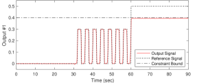
Figure 1: The system’s first output signal with DR/O-SDDPC.

V Conclusions

We proposed a Stochastic Data-Driven Predictive Control (SDDPC) method that accommodates distributionally robust (DR) probability constraints and produces closed-loop control policies with feedback gains determined from optimization. In theory, our SDDPC method can produce equivalent control inputs with associated Stochastic MPC, under specific conditions. Simulation results indicated separate benefits of using DR constraints and optimized feedback gains.

Appendix A Definition of $\Delta^{\sf U}_{i}$, $\Delta^{\sf Y}_{i}$, $\Delta^{\sf A}_{i}$, $\Delta^{\sf M}$

The matrices $\Delta^{\sf U}_{i}\in{}^{m\times mN},\Delta^{\sf Y}_{i}\in{}^{p\times mN},\Delta^{\sf A}_{i}\in{}^{p\times n_{\eta}}$ for $i\in\mathbb{Z}_{[0,N)}$ and $\Delta^{\sf M}\in{}^{pN\times n_{\eta}}$ in (14) are what follows,

$$\begin{aligned} &\mathrm{col}\big{(}\Delta^{\sf U}_{0},\ldots,\Delta^{\sf U}_{N-1}\big{)}:=I_{mN}\\ &\mathrm{col}\big{(}\Delta^{\sf Y}_{0},\ldots,\Delta^{\sf Y}_{N-1}\big{)}:=\Xi(A)\,(I_{N}\otimes B)\\ &\mathrm{col}\big{(}\Delta^{\sf A}_{0},\ldots,\Delta^{\sf A}_{N-1}\big{)}:=[\Theta(A),\Xi(A),I_{pN}]\\ &\Delta^{\sf M}:=[\Theta(A_{\sf L}),\Xi(A_{\sf L}),I_{pN}-\Xi(A_{\sf L})\,(I_{N}\otimes L_{\sf L})]\end{aligned}$$

where we let $\Theta(A):=\mathrm{col}(C,CA,\ldots,CA^{N-1})\in{}^{pN\times n}$, $\Xi(A):=\mathrm{Toep}(0_{p\times n},C,CA,\ldots,CA^{N-2})\in{}^{pN\times nN}$, and similarly define $\Theta(A_{\sf L}),\Xi(A_{\sf L})$ with $A_{\sf L}:=A-L_{\sf L}C$.

The matrices $\mathbf{\Delta}^{\sf U}_{i},\mathbf{\Delta}^{\sf Y}_{i},\mathbf{\Delta}^{\sf A}_{i},\mathbf{\Delta}^{\sf M}$ in (36) are computed (with underlying $\mathbf{\Theta}(\mathbf{A}),\mathbf{\Xi}(\mathbf{A}),\mathbf{A}_{\sf L}$) in the same way as above, with $A,B,C,L_{\sf L},n$ replaced by $\mathbf{A},\mathbf{B},\mathbf{C},\mathbf{L}_{\sf L},n_{\sf aux}$, respectively.

Appendix B Proof of (40)

Proof.

The relation $\accentset{\rule{2.79996pt}{0.8pt}}{y}_{t}=\accentset{\rule{2.79996pt}{0.8pt}}{\mathbf{y}}_{t}$ in (40) was established in [16, Claim 7.7]. The other relation in (40) is equivalent to

$$\begin{aligned} \Delta^{\sf U}_{t-k}&=\mathbf{\Delta}^{\sf U}_{t-k},&\Delta^{\sf M}\Sigma^{\eta}(\Delta^{\sf M})^{\sf T}&=\mathbf{\Delta}^{\sf M}\mathbf{\Sigma}^{\eta}(\mathbf{\Delta}^{\sf M})^{\sf T},\\ \Delta^{\sf Y}_{t-k}&=\mathbf{\Delta}^{\sf Y}_{t-k},&\Delta^{\sf A}_{t-k}\Sigma^{\eta}(\Delta^{\sf A}_{t-k})^{\sf T}&=\mathbf{\Delta}^{\sf A}_{t-k}\mathbf{\Sigma}^{\eta}(\mathbf{\Delta}^{\sf A}_{t-k})^{\sf T},\end{aligned}$$

via the definitions of $\Lambda_{t}$ and $\mathbf{\Lambda}_{t}$ in (14) and (36). Given the definitions in Appendix A, the above relations are implied by

1. $CA^{q}B=\mathbf{C}\mathbf{A}^{q}\mathbf{B}$ for $q\in\mathbb{Z}_{[0,N)}$,

2. $CA^{q}\Sigma^{\sf x}(CA^{r})^{\sf T}=\mathbf{C}\mathbf{A}^{q}\mathbf{\Sigma}^{\sf x}(\mathbf{C}\mathbf{A}^{r})^{\sf T}$ for $q,r\in\mathbb{Z}_{[0,N)}$,

3. $CA^{q}\Sigma^{\sf w}(CA^{r})^{\sf T}=\mathbf{C}\mathbf{A}^{q}\mathbf{\Sigma}^{\sf w}(\mathbf{C}\mathbf{A}^{r})^{\sf T}$ for $q,r\in\mathbb{Z}_{[0,N-2]}$,

4. $CA_{\sf L}^{q}\Sigma^{\sf x}(CA_{\sf L}^{q})^{\sf T}=\mathbf{C}\mathbf{A}_{\sf L}^{q}\mathbf{\Sigma}^{\sf x}(\mathbf{C}\mathbf{A}_{\sf L}^{r})^{\sf T}$ for $q,r\in\mathbb{Z}_{[0,N)}$,

5. $CA_{\sf L}^{q}\Sigma^{\sf w}(CA_{\sf L}^{q})^{\sf T}=\mathbf{C}\mathbf{A}_{\sf L}^{q}\mathbf{\Sigma}^{\sf w}(\mathbf{C}\mathbf{A}_{\sf L}^{r})^{\sf T}$ for $q,r\in\mathbb{Z}_{[0,N-2]}$,

6. $CA_{\sf L}^{q}L_{\sf L}=\mathbf{C}\mathbf{A}_{\sf L}^{q}\mathbf{L}_{\sf L}$ for $q\in\mathbb{Z}_{[0,N-2]}$,

where the relations 1)–6) can be shown given the equalities

$$\begin{aligned} A\Phi\Phi_{\sf aux}&=\Phi\mathbf{A}\Phi_{\sf aux},&B&=\Phi\mathbf{B},&L_{\sf L}&=\Phi\mathbf{L}_{\sf L},\\ \mathbf{A}\Phi_{\sf aux}&=\Phi_{\sf aux}\widetilde{A},&\mathbf{B}&=\Phi_{\sf aux}\widetilde{B},&\mathbf{L}_{\sf L}&=\Phi_{\sf aux}\widetilde{L}_{\sf L},\\ C\Phi\Phi_{\sf aux}&=\mathbf{C}\Phi_{\sf aux},&\Sigma^{\sf w}&=\Phi\mathbf{\Sigma}^{\sf w}\Phi^{\sf T},&\Sigma^{\sf x}&=\Phi\mathbf{\Sigma}^{\sf x}\Phi^{\sf T},\end{aligned}$$

established with some matrices $\Phi,\widetilde{A},\widetilde{B},\widetilde{L}_{\sf L}$ according to [16, Claim 5.1, Claim 7.1, Claim 7.4]. ∎

References

• [1] D. Q. Mayne, “Model predictive control: Recent developments and future promise,” Automatica, vol. 50, no. 12, pp. 2967–2986, 2014.
• [2] A. Bemporad and M. Morari, “Robust model predictive control: A survey,” in Robustness in identification and control.   Springer, 2007, pp. 207–226.
• [3] A. Mesbah, “Stochastic model predictive control: An overview and perspectives for future research,” IEEE Control Syst. Mag., vol. 36, no. 6, pp. 30–44, 2016.
• [4] R. Kumar, J. Jalving, M. J. Wenzel, M. J. Ellis, M. N. ElBsat, K. H. Drees, and V. M. Zavala, “Benchmarking stochastic and deterministic MPC: a case study in stationary battery systems,” AIChE Journal, vol. 65, no. 7, p. e16551, 2019.
• [5] F. Dörfler, “Data-driven control: Part two of two: Hot take: Why not go with models?” IEEE Control Syst. Mag., vol. 43, no. 6, pp. 27–31, 2023.
• [6] Z.-S. Hou and Z. Wang, “From model-based control to data-driven control: Survey, classification and perspective,” Inf. Sci., vol. 235, pp. 3–35, 2013.
• [7] J. Coulson, J. Lygeros, and F. Dörfler, “Data-enabled predictive control: In the shallows of the DeePC,” in Proc. ECC, 2019, pp. 307–312.
• [8] ——, “Regularized and distributionally robust data-enabled predictive control,” in Proc. IEEE CDC, 2019, pp. 2696–2701.
• [9] ——, “Distributionally robust chance constrained data-enabled predictive control,” IEEE Trans. Autom. Control, vol. 67, no. 7, pp. 3289–3304, 2021.
• [10] B. Huang and R. Kadali, Dynamic modeling, predictive control and performance monitoring: a data-driven subspace approach.   Springer, 2008.
• [11] E. Elokda, J. Coulson, P. N. Beuchat, J. Lygeros, and F. Dörfler, “Data-enabled predictive control for quadcopters,” Int. J. Robust Nonlinear Control, vol. 31, no. 18, pp. 8916–8936, 2021.
• [12] P. G. Carlet, A. Favato, S. Bolognani, and F. Dörfler, “Data-driven predictive current control for synchronous motor drives,” in ECCE, 2020, pp. 5148–5154.
• [13] L. Huang, J. Coulson, J. Lygeros, and F. Dörfler, “Decentralized data-enabled predictive control for power system oscillation damping,” IEEE Trans. Control Syst. Tech., vol. 30, no. 3, pp. 1065–1077, 2021.
• [14] G. Pan, R. Ou, and T. Faulwasser, “Towards data-driven stochastic predictive control,” Int. J. Robust Nonlinear Control, 2022.
• [15] ——, “On a stochastic fundamental lemma and its use for data-driven optimal control,” IEEE Trans. Autom. Control, 2022.
• [16] R. Li, J. W. Simpson-Porco, and S. L. Smith, “Stochastic data-driven predictive control with equivalence to stochastic MPC,” arXiv preprint arXiv:2312.15177, 2023.
• [17] B. P. Van Parys, D. Kuhn, P. J. Goulart, and M. Morari, “Distributionally robust control of constrained stochastic systems,” IEEE Trans. Autom. Control, vol. 61, no. 2, pp. 430–442, 2015.
• [18] S. Zymler, D. Kuhn, and B. Rustem, “Distributionally robust joint chance constraints with second-order moment information,” Math. Program., vol. 137, pp. 167–198, 2013.
• [19] M. Farina, L. Giulioni, L. Magni, and R. Scattolini, “An approach to output-feedback MPC of stochastic linear discrete-time systems,” Automatica, vol. 55, pp. 140–149, 2015.
• [20] E. Joa, M. Bujarbaruah, and F. Borrelli, “Output feedback stochastic mpc with hard input constraints,” in Proc. ACC, 2023, pp. 2034–2039.
• [21] J. Ridderhof, K. Okamoto, and P. Tsiotras, “Chance constrained covariance control for linear stochastic systems with output feedback,” in Proc. IEEE CDC, 2020, pp. 1758–1763.
• [22] P. J. Goulart and E. C. Kerrigan, “Output feedback receding horizon control of constrained systems,” Int J Control, vol. 80, no. 1, pp. 8–20, 2007.
• [23] J. Humpherys, P. Redd, and J. West, “A fresh look at the kalman filter,” SIAM review, vol. 54, no. 4, pp. 801–823, 2012.
• [24] L. E. Ghaoui, M. Oks, and F. Oustry, “Worst-case value-at-risk and robust portfolio optimization: A conic programming approach,” Oper. Res., vol. 51, no. 4, pp. 543–556, 2003.
• [25] H. Ye, “Scheduling of networked control systems,” IEEE Control Syst., vol. 21, no. 1, pp. 57–65, 2001.
• [26] C. De Persis and P. Tesi, “Formulas for data-driven control: Stabilization, optimality, and robustness,” IEEE Trans. Autom. Control, vol. 65, no. 3, pp. 909–924, 2019.