Better bounds on Grothendieck constants of finite orders

Abstract

Grothendieck constants $K_{G}\left({d}{}\right)$ bound the advantage of $d$-dimensional strategies over $1$-dimensional ones in a specific optimisation task. They have applications ranging from approximation algorithms to quantum nonlocality. However, apart from $d=2$, their values are unknown. Here, we exploit a recent Frank-Wolfe approach to provide good candidates for lower bounding some of these constants. The complete proof relies on solving difficult binary quadratic optimisation problems. For $d\in\{3,4,5\}$, we construct specific rectangular instances that we can solve to certify better bounds than those previously known; by monotonicity, our lower bounds improve on the state of the art for $d\leqslant 9$. For $d\in\{4,7,8\}$, we exploit elegant structures to build highly symmetric instances achieving even greater bounds; however, we can only solve them heuristically. We also recall the standard relation with violations of Bell inequalities and elaborate on it to interpret generalised Grothendieck constants $K_{G}\left({d}\mapsto{2}\right)$ as the advantage of complex quantum mechanics over real quantum mechanics. Motivated by this connection, we also improve the bounds on $K_{G}\left({d}\mapsto{2}\right)$.

I Introduction

Published in French in a Brazilian journal, Grothendieck’s pioneering work on Banach spaces from 1953 Gro53 , now informally known as his Résumé, has long remained unnoticed. In 1968, Lindenstrauss and Pełczyński LP68 discovered it and rephrased the main result, the Grothendieck inequality, which proves a relationship between three fundamental tensor norms through the so-called Grothendieck constant, denoted $K_{G}$. Since then, this far-reaching theorem has found numerous applications Pis11 , in particular in combinatorial optimisation where it is at the heart of an algorithm to approximate the cut-norm of a matrix KN12 .

Quantum information is another field where this result is influential: following early observations by Tsirelson Tsi87 , an explicit connection has been established with the noise robustness in Bell experiments Bel64 ; AGT06 . These experiments aim at exhibiting a fascinating property of quantum mechanics in correlation scenarios: nonlocality BCP+14 . The link with Grothendieck’s theorem has then raised a surge of interest for the value of $K_{G}\left({3}{}\right)$, the Grothendieck constant of order three. Many works have thus demonstrated increasingly precise lower bounds CHSH69 ; Ver08 ; HLZ+15 ; BNV16 ; DBV17 ; DIB+23 and upper bounds Kri79 ; HQV+17 ; DIB+23 on its value. More recently, a numerical method has also been developed to come up with an even more precise (but not provable) estimate of $K_{G}\left({3}{}\right)$ SM24 .

For Grothendieck constants of higher orders, the link with quantum nonlocality remains AGT06 ; VP08 . However, the bounds on their values have been less studied and are less tight Kri79 ; FR94 ; Ver08 ; BBT11 ; HLZ+15 ; DBV17 . There are quite a few difficulties that explain this relative scarcity of results, many of them being manifestations of the curse of dimensionality. Finding suitable high-dimensional ansätze indeed becomes increasingly hard and resulting instances involve sizes that rapidly become intractable.

In this article, we combine the recent projection technique from DIB+23 with the powerful solver developed in DBV17 to obtain better lower bounds on $K_{G}\left({d}{}\right)$ for $3\leqslant d\leqslant 9$. Following FR94 , we also consider symmetric structures in high dimensions emerging from highly symmetric line packings FJM18 to suggest even better bounds on $K_{G}\left({4}{}\right)$, $K_{G}\left({7}{}\right)$, and $K_{G}\left({8}{}\right)$, that we unfortunately cannot prove as they involve optimisation problems that we only solve heuristically. We also consider the generalised Grothendieck constants $K_{G}\left({d}\mapsto{2}\right)$ and interpret them as the advantage of $d$-dimensional quantum mechanics over real quantum mechanics, a fact that was already studied in VP08 ; VP09 , but recently received more attention through the powerful results of RTW+21 . Our bounds on $K_{G}\left({d}{}\right)$ are analytical, while those on $K_{G}\left({d}\mapsto{2}\right)$ strongly rely on numerical methods: we post-process the upper bound on $K_{G}\left({3}\mapsto{2}\right)$ to convert it into an exact result, but the lower bounds remain inaccurate.

We first formally define the constants we want to bound in Section II before presenting in Section III our method and main results on lower bounds on $K_{G}\left({d}{}\right)$, summarised in Tables 1 and 2. Then we turn to generalised constants in Section IV, where we review existing bounds before deriving ours, which are particularly tight on the value of $K_{G}\left({3}\mapsto{2}\right)$. Finally, we recall the connection with quantum mechanics in Section IV.4 and conclude in Section V.

II Preliminaries

Given a real matrix $M$ of size $m_{1}\times m_{2}$, we define

$$\mathrm{SDP}_{d}\left({M}\right)=\max\left\{\sum_{x=1}^{m_{1}}\sum_{y=1}^{m_{2}}M_{xy}\left\langle{a_{x}},{b_{y}}\right\rangle\leavevmode\nobreak\ \Big{|}\leavevmode\nobreak\ \forall x\in[m_{1}],\leavevmode\nobreak\ a_{x}\in S^{d-1},\leavevmode\nobreak\ \forall y\in[m_{2}],\leavevmode\nobreak\ b_{y}\in S^{d-1}\right\},$$ (1)

where $[m]=\{1,\ldots,m\}$ and where $S^{d-1}$ is the $d$-dimensional unit sphere, which reduces to $S^{0}=\{-1,1\}$ for $d=1$. By introducing the set

$$\mathrm{SDP}_{d}^{m_{1},m_{2}}=\operatorname{conv}\left\{X\leavevmode\nobreak\ \big{|}\leavevmode\nobreak\ X_{xy}=\left\langle{a_{x}},{b_{y}}\right\rangle,\leavevmode\nobreak\ \forall x\in[m_{1}],\leavevmode\nobreak\ a_{x}\in S^{d-1},\leavevmode\nobreak\ \forall y\in[m_{2}],\leavevmode\nobreak\ b_{y}\in S^{d-1}\right\},$$ (2)

we get the equivalent definition

$$\mathrm{SDP}_{d}\left({M}\right)=\max\left\{\left\langle{M},{X}\right\rangle\leavevmode\nobreak\ \big{|}\leavevmode\nobreak\ X\in\mathrm{SDP}_{d}^{m_{1},m_{2}}\right\}.$$ (3)

The reason for this name comes from the interpretation of the Grothendieck constant that we are about to define in the context of rank-constrained semidefinite programming BOV14 . In the following, when $m_{1}=m_{2}$, we simply write $\mathrm{SDP}_{d}^{m,m}=\mathrm{SDP}_{d}^{m}$; also, when the size $m_{1},m_{2}$ is either clear from the context of irrelevant, we will use the shorthand notation $\mathrm{SDP}_{d}^{m_{1},m_{2}}=\mathrm{SDP}_{d}$.

In essence, the Grothendieck inequality states that there exists a (finite) constant independent of the size of the matrix $M$ that bounds the ratio between the quantities $\mathrm{SDP}_{d}\left({M}\right)$ for various $d$. More formally, given $n\leqslant d$, for all real matrices $M$, we have Gro53

$$\mathrm{SDP}_{d}\left({M}\right)\leqslant K_{G}\left({d}\mapsto{n}\right)\mathrm{SDP}_{n}\left({M}\right),$$ (4)

so that the exact definition of these generalised Grothendieck constants is

$$K_{G}\left({d}\mapsto{n}\right)=\sup\left\{\frac{\mathrm{SDP}_{d}\left({M}\right)}{\mathrm{SDP}_{n}\left({M}\right)}\leavevmode\nobreak\ \Big{|}\leavevmode\nobreak\ M\in\mathbb{R}^{m_{1}\times m_{2}},\quad m_{1},m_{2}\in\mathbb{N}\right\}.$$ (5)

The standard Grothendieck constant of order $d$ is obtained when $n=1$, in which case we use the shorthand notation $K_{G}\left({d}\mapsto{1}\right)=K_{G}\left({d}{}\right)$. The Grothendieck constant of infinite order $K_{G}$ initially studied in Gro53 corresponds to the limit $\lim_{d\rightarrow\infty}K_{G}\left({d}{}\right)$, but it is out of the scope of our work, although we briefly mention it in Section V. We refer the reader interested in general aspects and further generalisations of these constants to Bri11 .

III Lower bounds on $K_{G}\left({d}{}\right)$

Given the definition of $K_{G}\left({d}{}\right)$ in Eq. 5, any matrix $M$ automatically provides a valid lower bound. However, there are two main difficulties when looking for good lower bounds.

Problem 1.

Given $m_{1}$ and $m_{2}$, how to find a matrix $M$ such that the inequality in Eq. 4 is as tight as possible?

Problem 2.

Given such a matrix $M$, how to compute the resulting $\mathrm{SDP}_{1}\left({M}\right)$ or at least a close upper bound?

2 is the most limiting one, as the computation of $\mathrm{SDP}_{1}\left({M}\right)$ is equivalent to MaxCut and therefore NP-hard, so that the size of the matrices to consider are limited by the methods and resources available to compute this number. In general, solving 1 exactly is out of reach, but good candidates can be found and this suffices to derive bounds.

In the rest of this section, we first recall the method from DIB+23 to both problems above, in particular to 1. To illustrate the idea of the method, we give up on solving 2 for the sake of the elegance of the solution to 1, providing instances of remarkable symmetry for which future works may solve 2 to improve on the bounds on $K_{G}\left({4}{}\right)$, $K_{G}\left({7}{}\right)$, and $K_{G}\left({8}{}\right)$. We then focus on 2 and consider rectangular matrices allowing us to obtain certified bounds on $K_{G}\left({3}{}\right)$, $K_{G}\left({4}{}\right)$, and $K_{G}\left({5}{}\right)$ that beat the literature up to $d=9$, by monotonicity.

III.1 Obtaining facets of the symmetrised correlation polytope

When $n=1$, the set $\mathrm{SDP}_{1}$ is a polytope, called the correlation polytope Pit91 . In BNV16 ; DBV17 ; DIB+23 the method used to solve 1 is to start from a point $P\in\mathrm{SDP}_{d}$ and to derive $M$ as a hyperplane separating $P$ from $\mathrm{SDP}_{1}$. This hyperplane is obtained by solving the projection of $P$ onto the correlation polytope $\mathrm{SDP}_{1}$ via Frank-Wolfe algorithms. We refer to Pok23 for a gentle introduction to FW algorithms, to BCC+22 for a complete review, and to (DIB+23, , Appendix C) for the details of our implementation. Note that some accelerations developed in DIB+23 ; DVP24 and used in this work are now part of the FrankWolfe.jl package BDH+24 .

In particular, the symmetrisation described in DVP24 is crucial, but as it depends on the underlying group and its action of the matrices we consider, exposing the full structure of the symmetrised correlation polytope for each group would be tedious. Instead, we give an brief general definition of this polytope and refer to DVP24 for a detailed example. Given a group $G$ acting on $[m_{1}]$ and $[m_{2}]$ (by means of signed permutations), the symmetrised correlation polytope $G(\mathrm{SDP}_{1}^{m_{1},m_{2}})$ is the convex hull of the averages of all orbits of the vertices of $\mathrm{SDP}_{1}^{m_{1},m_{2}}$ under the action of $G$. Note that this polytope lives in a subspace of the space invariant under the action of $G$ on matrices of size $m_{1}\times m_{2}$.

In Fig. 1 we illustrate the various geometrical cases that we encounter in this work. Their understanding justifies the procedure that we describe in Algorithm 1 to derive facets of the symmetrised correlation polytope, that is, separating hyperplanes touching the polytope on a space of codimension one. Importantly, for symmetric instances, the dimension of the ambient space is strictly smaller than $m_{1}m_{2}$. In the following, we consistently denote these facets by $A$, while $M$ will indicate separating hyperplanes without this extra property. Putative facets will also be denoted by $A$, that is, in cases where we rely on heuristic methods to compute $\mathrm{SDP}_{1}\left({A}\right)$.

These heuristic methods play an important role throughout the FW algorithm as they quickly give a good direction to make primal progress. Here we present them in a generalised framework that will turn useful when generalising our algorithm to $K_{G}\left({d}\mapsto{2}\right)$ in Section IV. At a given step of the FW algorithm minimising the squared distance to the set $\mathrm{SDP}_{n}$, finding the best direction with respect to the current gradient $M$ is exactly the problem in Eq. 3. This subroutine is called the Linear Minimisation Oracle (LMO) and, in the course of the algorithm, we usually use an alternating minimisation to obtain heuristic solutions that are enough to make progress (DIB+23, , Appendix B.1).

More formally, for all $x\in[m_{1}]$, we pick a random $a^{h}_{x}\in S^{n-1}$ and we compute, for all $y\in[m_{2}]$,

$$b^{h}_{y}=\operatorname*{arg\,max}_{b_{y}\in S^{n-1}}\sum_{y=1}^{m_{2}}b_{y}\bigg{(}\sum_{x=1}^{m_{1}}M_{xy}a^{h}_{x}\bigg{)},\qquad\text{that is,}\qquad b^{h}_{y}=\frac{\sum_{\vphantom{y}x=1}^{m_{1}}M_{xy}a^{h}_{x}}{\left\|\sum_{\vphantom{y}x=1}^{m_{1}}M_{xy}a^{h}_{x}\right\|}.$$ (6)

In the unlikely case where the denominator happens to be zero, we set $b^{h}_{y}$ to be a predetermined vector, for instance, $(1,0,\ldots,0)\in S^{n-1}$. Similarly, we then use these $b^{h}_{y}$ to compute

$$a^{h}=\operatorname*{arg\,max}_{a_{x}\in S^{n-1}}\sum_{x=1}^{m_{1}}a_{x}\bigg{(}\sum_{y=1}^{m_{2}}M_{xy}b^{h}_{y}\bigg{)},\qquad\text{that is,}\qquad a^{h}_{x}=\frac{\sum_{y=1}^{m_{2}}M_{xy}b^{h}_{y}}{\left\|\sum_{y=1}^{m_{2}}M_{xy}b^{h}_{y}\right\|},$$ (7)

and we repeat Eqs. 6 and 7 until the objective value in Eq. 1 stops increasing, up to numerical precision when $n>1$. Depending on the initial choice of $a^{h}_{x}$, the value attained will vary. Therefore we restart the procedure a large number of times: from a few hundreds or thousands within the FW algorithm, to $10^{5}$ in Table 4 and $10^{8}$ in Table 1.

In the following, we clearly mention when the last part of our method — the computation of $\mathrm{SDP}_{1}\left({M}\right)$ (or $\mathrm{SDP}_{2}\left({M}\right)$ in Section IV) where $M$ is the last gradient return by our FW algorithm — is done with the heuristic procedure just described, which comes with no theoretical guarantee, or with a more elaborate solver for which the exact value can be certified or rigourously upper bounded.

(a)

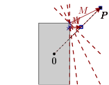
(b)

(c)

(d)

Figure 1: Illustration of our projection method to separate a matrix $P\in\mathrm{SDP}_{d}$ from the correlation polytope $\mathrm{SDP}_{1}$. (a) In all cases that we consider in this work, the direction $P$ already defines, together with the corresponding value of $\mathrm{SDP}_{1}\left({P}\right)$, a separating hyperplane. (b) When running our FW algorithm to minimise the distance between $P$ and $\mathrm{SDP}_{1}$, the orthogonal projection obtained does not, in general, lie on a facet. The resulting separating hyperplane $M$ is better than $P$ from (a), but still not optimal. Note that this situation can also happen when starting from a point $vP$ on the line $[0,P]$ that is not close enough to $\mathrm{SDP}_{1}$ (not depicted here). (c) Even when $v$ is chosen small enough, if our FW algorithm has not fully converged to the orthogonal projection of $vP$, the separating hyperplane $M$ slightly deviates from a facet. (d) For a small enough $v$ and when our FW algorithm has converged, the resulting separating hyperplane is a facet, denoted $A$, that is, the tightest separation leading to the best value of $\left\langle{A},{P}\right\rangle/\mathrm{SDP}_{1}\left({A}\right)$.

Algorithm 1 Iterative procedure to derive a facet via the Blended Pairwise Conditional Gradient (BPCG) algorithm

1:Input: $P\in\mathrm{SDP}_{d}^{m_{1},m_{2}}$

2:$v\leftarrow 1$ $\triangleright$ $P$ assumed outside of $\mathrm{SDP}_{1}^{m_{1},m_{2}}$, see Fig. 1a

3:$\mathcal{S}\leftarrow\varnothing$ $\triangleright$ empty active set to start with

4:while $\operatorname{codim}\mathcal{S}>1$ do $\triangleright$ dimension of the subspace generated by the active set

5:     $X,\mathcal{S}\leftarrow\mathrm{BPCG}(vP)$ $\triangleright$ $X$ is the projection of $vP$ onto $\mathrm{SDP}_{1}^{m_{1},m_{2}}$ obtained with Algorithm 2 from DIB+23

6:     $M\leftarrow vP-X$ $\triangleright$ direction of the separating hyperplane given by the final gradient

7:     $v\leftarrow\left\langle{M},{P}\right\rangle/\mathrm{SDP}_{1}\left({M}\right)$ $\triangleright$ new point on the line $[0,P]$, strictly closer to $\mathrm{SDP}_{1}^{m_{1},m_{2}}$ than the previous one

8:end while$\triangleright$ $\operatorname{codim}\mathcal{S}=1$, the ambient dimension may be smaller than $m_{1}m_{2}$ by symmetry

9:Output: $A\perp\mathcal{S}$ $\triangleright$ normal vector defining the facet $A$ of the symmetrisation of $\mathrm{SDP}_{1}^{m_{1},m2}$ BBB+12 ; DVP24

III.2 Heuristic results with highly symmetric line packings

Starting from a good point $P\in\mathrm{SDP}_{d}$ in the procedure described above is key to obtaining good bounds on $K_{G}\left({d}{}\right)$. Following DBV17 , we observed that spanning the $d$-dimensional projective unit sphere in the most uniform way seems to be favourable, which served as our guiding principle to come up with structures in higher dimensions. In this Section III.2, we use the same distribution of points on both sides in Eq. 2, that is, $m_{1}=m_{2}=m$ and $a_{1}=b_{1},\ldots a_{m}=b_{m}$; the matrix $P$ is therefore a Gram matrix.

The intuitive but vague notion of uniform spreading on the sphere can be formally seen as the problem of finding good line packings CHS96 ; FJM18 . In Table 1, for various symmetric $d$-dimensional line packings, we give the values of $\mathrm{SDP}_{d}\left({P}\right)/\mathrm{SDP}_{1}\left({P}\right)$ and $\mathrm{SDP}_{d}\left({A}\right)/\mathrm{SDP}_{1}\left({A}\right)$. Since the Gram matrix $P$ is positive semidefinite, the ratio $\mathrm{SDP}_{d}\left({P}\right)/\mathrm{SDP}_{1}\left({P}\right)$ is upper bounded by $K_{G}^{\succeq}(d)$, the positive semidefinite Grothendieck constant of order $d$ BOV10 , whose value is known to be $\gamma(d)\pi/2$ (Bri11, , Theorem 4.1.3), where $\gamma(d)$ is defined in Eq. 10 below. Note that, for $d\geqslant 9$, this bound is the current best known lower bound on $K_{G}\left({d}{}\right)$ which is naturally greater than $K_{G}^{\succeq}(d)$.

Among the structures that we present in Table 1, the $d$-dimensional configurations reaching the best known kissing number in dimension $d$ are of particular interest. In particular, in dimension $d=3$, different realisations of the kissing number give rise to different values of $\mathrm{SDP}_{3}\left({A}\right)/\mathrm{SDP}_{1}\left({A}\right)$. As the icosahedron is an optimal line packing, this indicates that giving good bounds on $K_{G}\left({d}{}\right)$ does not, in general, boil down to finding good line packings. Note that the unicity of the configuration in dimension $d=4$ was recently proven LLM24 .

Upon inspection of Table 1 it is apparent that, in the small dimensions that we consider in this work ($d\leqslant 8$), root systems play an important role in obtaining good kissing configurations. These structures are inherently symmetric and play an important role in the theory of Lie groups and Lie algebras. We refer to Bak02 for definitions and elementary properties. The family $D_{d}$ has been studied in FR94 ; there, starting from the Gram matrix $P$ of size $d(d-1)$, the exact value of $\mathrm{SDP}_{1}\left({P}\right)$ is computed by invoking symmetry arguments. Moreover, for $d\in\{3,4,5\}$, the optimal diagonal modification of $\lambda=\frac{2}{3}$ is derived for $D_{d}$; in other words, FR94 shows that, among all matrices with shape $P-\lambda\mathds{1}$, the matrix $P-\frac{2}{3}\mathds{1}$ is giving the best lower bound on $K_{G}\left({d}{}\right)$. Here we go a bit further by extending this result to $d\in\{6,7,8\}$, a fact that was suspected in FR94 , but we also observe that the corresponding matrices $A=P-\frac{2}{3}\mathds{1}$ are actually facets of the symmetrised polytope $D_{d}(\mathrm{SDP}_{1}^{d(d-1)})$.

Moreover, we computationnally establish optimal diagonal modifications for other configurations, see Table 1. About the root system $E_{8}$, we note that the value $45/31$ reached without diagonal modification is already provided in (FR94, , page 50), where it is attributed to Reeds and Sloane. It indeed follows from (FR94, , Lemma 2) and from the transitivity of the Weyl group, see the acknowledgements in Section VII. However, these arguments do not directly apply to solve the diagonally modified case.

Note that in all cases involving irrational numbers (except the icosahedron), the facet $A$ cannot be obtained via a diagonal modification of $P$. This is because the off-diagonal elements of $P$ feature rational and irrational numbers. The exception of the icosahedron is due to its extra property of being an equiangular tight frame (ETF), all off-diagonal elements being $\pm 1/\sqrt{5}$, which can then lead to a facet by taking an irrational diagonal modification.

$d$	$m$	$\frac{\mathrm{SDP}_{d}\left({P}\right)}{\mathrm{SDP}_{1}\left({P}\right)}$		$\frac{\mathrm{SDP}_{d}\left({A}\right)}{\mathrm{SDP}_{1}\left({A}\right)}\geqslant$		Comments	Kissing	$G$	$\lambda$
2	3	$\frac{9}{8}$	$=1.125$	$\frac{5}{4}$	$=1.25\hphantom{00^{*}}$ DVP24	Hexagon	x	$A_{2}$	$\frac{2}{3}$
		$\frac{9-3\sqrt{5}}{2}$	$\approx 1.1459\hphantom{{}^{*}}$ PV22	$\frac{1+3\sqrt{5}}{6}$	$\approx 1.2847$	Icosahedron	x	$H_{3}$	$\frac{15-\sqrt{5}}{15}$
	6	$\frac{6}{5}$	$=1.2\hphantom{000^{*}}$ FR94	$\frac{4}{3}$	$\approx 1.3333\hphantom{{}^{*}}$ FR94	Cuboctahedron	x	$A_{3}$	$\frac{2}{3}$
	10	$\frac{25(7-3\sqrt{5})}{6}$	$\approx 1.2158\hphantom{{}^{*}}$ PV22	$\frac{7+3\sqrt{5}}{10}$	$\approx 1.3708$	Dodecahedron
3	15	$\frac{75(31-12\sqrt{5})}{241}$	$\approx 1.2968\hphantom{{}^{*}}$	$\frac{5\sqrt{5}}{8}$	$\approx 1.3975$	Icosidodecahedron		$H_{3}$
	12	$\frac{9}{7}$	$\approx 1.2857\hphantom{{}^{*}}$ FR94	$\frac{7}{5}$	$=1.4\hphantom{000^{*}}$ FR94	24-cell	x	$D_{4}$	$\frac{2}{3}$
	60	$\frac{225(83-36\sqrt{5})}{409}$	$\approx 1.3762\hphantom{{}^{*}}$ PV22	$\frac{100(16+15\sqrt{5})}{3361}$	$\approx 1.4740$	600-cell
4	300	$\frac{225(1635-731\sqrt{5})}{71}$	$\approx 1.3763\hphantom{{}^{*}}$ PV22	$\frac{3(\alpha+\beta\sqrt{5})}{\gamma}$	$\approx 1.4996^{*}$	120-cell		$H_{4}$
5	20	$\frac{4}{3}$	$\approx 1.3333\hphantom{{}^{*}}$ FR94	$\frac{10}{7}$	$\approx 1.4286\hphantom{{}^{*}}$ FR94		x	$D_{5}$	$\frac{2}{3}$
	30	$\frac{15}{11}$	$\approx 1.3636\hphantom{{}^{*}}$ FR94	$\frac{13}{9}$	$\approx 1.4444$			$D_{6}$	$\frac{2}{3}$
6	36	$\frac{18}{13}$	$\approx 1.3846$	$\frac{16}{11}$	$\approx 1.4545$		x	$E_{6}$	$\frac{2}{3}$
	28	$\frac{28}{25}$	$=1.12$	$\frac{133}{109}$	$\approx 1.2202$	ETF LS66			$\frac{39}{24}$
	42	$\frac{18}{13}$	$\approx 1.3846\hphantom{{}^{*}}$ FR94	$\frac{16}{11}$	$\approx 1.4545$			$D_{7}$	$\frac{2}{3}$
	63	$\frac{27}{19}$	$\approx 1.4211$	$\frac{2961}{1991}$	$\approx 1.4872$		x	$E_{7}$	$\frac{7}{6}$
7	91	$\frac{3549(1433-604\sqrt{3})}{959041}$	$\approx 1.4315^{*}$	$\frac{24631+18216\sqrt{3}}{37463}$	$\approx 1.4997^{*}$	E7 + ETF FJM18
	56	$\frac{7}{5}$	$=1.4\hphantom{000^{*}}$ FR94	$\frac{19}{13}$	$\approx 1.4615$			$D_{8}$	$\frac{2}{3}$
8	120	$\frac{45}{31}$	$\approx 1.4516\hphantom{{}^{*}}$ FR94	$\frac{165}{109}$	$\approx 1.5138^{*}$		x	$E_{8}$	$\frac{13}{6}$

Table 1: Lower bounds on $K_{G}\left({d}{}\right)$ obtained via root systems and other remarkable configurations with symmetry group $G$. The matrix $A$ is the facet separating the Gram matrix $P$ of the configuration from the symmetrised correlation polytope $G(\mathrm{SDP}_{1})$. When $A=P-\lambda\mathds{1}$, we give the corresponding value of this diagonal modification FR94 in the last column. Shaded cells indicate potential improvements on the state of the art, but in most of these cases, the asterisk ^∗ indicates that our solution of $\mathrm{SDP}_{1}\left({A}\right)$ is heuristic, hence only putative, see Table 2a. Only the bound on $K_{G}\left({7}{}\right)$ obtained with the $E_{7}$ root system is both exact and good enough to beat the literature; below, by monotonicity of $K_{G}\left({d}{}\right)$, we further improve this bound, see Table 2b. For the 120-cell, we define $\alpha=2566372165103191$, $\beta=1178280120531798$, and $\gamma=10405220765436757$. Note that we are able to exactly obtain $\mathrm{SDP}_{d}\left({P}\right)$ as all these configurations satisfy the platonic property from PV22 . Moreover, we could numerically observe the tightness of our lower bound on $\mathrm{SDP}_{d}\left({A}\right)$ by computing the first level of the Lasserre hierarchy Las01 , see Section IV.2 below.

The 600-cell and the 120-cell have already been studied in PV22 , where symmetry arguments are exploited to compute the value of $\mathrm{SDP}_{1}\left({P}\right)$, even for the $300\times 300$ matrix arising from the 120-cell. Interestingly, although the difference of value for $\mathrm{SDP}_{4}\left({P}\right)/\mathrm{SDP}_{1}\left({P}\right)$ is almost negligible, the facets that we obtain here “activate” the advantage of the 120-cell. Also, we emphasise the advantage of our geometric approach for these structures: in PV22 , the optimal diagonal modification of $23/9$ was indeed derived for the 600-cell, giving rise the the value of $35(-37+27\sqrt{5})/569\approx 1.4378$, which is significantly smaller than our result of about $1.4740$, see Table 1. This is because we are not restricted to diagonal modifications in our algorithm, which gives a significant superiority for these configurations.

For some instances of $\mathrm{SDP}_{1}\left({P}\right)$ and $\mathrm{SDP}_{1}\left({A}\right)$, the size of the matrix is too large for numerical solvers to handle it. The values presented with an asterisk in Table 1 and summarised in Table 2a are then obtained heuristically and cannot be considered final results until these values are confirmed to be optimal. For this, the high symmetry of these instances, detrimental for our branch-and-bound algorithm and not exploited in available QUBO/MaxCut solvers, could play a crucial role. We leave this open for further research.

III.3 Exact results in asymmetric scenarios

Now, we discuss how to address 2, namely, the computation of

$$\mathrm{SDP}_{1}\left({M}\right)=\max_{\genfrac{}{}{0.0pt}{}{a_{x}=\pm 1}{b_{y}=\pm 1}}\sum_{x=1}^{m_{1}}\sum_{y=1}^{m_{2}}M_{xy}{a_{x}}{b_{y}}$$ (8)

In DIB+23 this problem is reformulated into a Quadratic Unconstrained Binary Optimisation (QUBO) instance, which is then given to the solver QuBowl from RKS22 . The instance solved there involves $m_{1}=m_{2}=97$ and is bigger than the ones from DBV17 (of maximal size $m_{1}=m_{2}=92$). However, it is worth noticing that the solution of the exact instance solved in DIB+23 stands out in the landscape of all binary variables. More precisely, the exact solution is likely to be unique and its value is far above the other feasible points, so that the solver could efficiently exclude vast portions of the search space. This empirical observation is supported by two facts: instances from later stages of convergence of the Frank-Wolfe method cannot be solved by QuBowl (even within ten times as much time), and the symmetric instance $A$ of size $63\times 63$ obtained from the $E_{7}$ root system (see Table 1) cannot be solved by QuBowl either, although it is way smaller.

Given these difficulties, we consider other formulations exploiting the specificities of the problem. In particular, the branch-and-bound algorithm from DBV17 works by breaking the symmetry between the binary variables $a_{x}$ and $b_{y}$ in Eq. 8, fixing the latter to obtain:

$$\mathrm{SDP}_{1}\left({M}\right)=\max_{a_{x}=\pm 1}\sum_{y=1}^{m_{2}}\left|\sum_{x=1}^{m_{1}}M_{xy}{a_{x}}\right|,$$ (9)

which has half as many variables. Importantly, the parameter $m_{2}$ plays a less critical role in the complexity of the resulting algorithm, which is indeed still exponential in $m_{1}$, but now linear in $m_{2}$. This suggests to use rectangular matrices $M$ in our procedure, with a large $m_{2}$ to increase the achievable lower bound on $K_{G}\left({d}{}\right)$ and a relatively small $m_{1}$ to maintain the possibility to solve 2, that is, to compute $\mathrm{SDP}_{1}\left({M}\right)$.

Such rectangular matrices can be obtained by following the procedure described in Section III.1 starting from rectangular matrices $P\in\mathrm{SDP}_{d}^{m_{1},m_{2}}$. Good starting points are still obtained by using well spread distribution on the sphere, but these distributions $a_{1},\ldots,a_{m_{1}}$ and $b_{1},\ldots,b_{m_{2}}$ are now different, so that the matrix $P$ with entries $\left\langle{a_{x}},{b_{y}}\right\rangle$ is not a Gram matrix any more. We give our best lower bounds on $K_{G}\left({d}{}\right)$ in Table 2b and present relevant details below. All matrices can be found in the supplementary files .

In dimension $d=3$, despite our efforts, we could not find a rectangular instance beating the $97\times 97$ from DIB+23 . However, the quantum point provided therein, namely, the polyhedron on the Bloch sphere consisting of $97$ pairs of antipodal points, is not the best quantum strategy to violate the inequality. By using the Lasserre hierarchy at its first level, we can indeed obtain a slightly better violation, hence a tighter lower bound on $K_{G}\left({3}{}\right)$. Summarising, with the matrix $M$ from DIB+23 that had been constructed starting from a Gram matrix $P\in\mathrm{SDP}_{3}^{97}$, we have:

• $\mathrm{SDP}_{3}\left({M}\right)\geqslant\left\langle{M},{P}\right\rangle\approx 2.0000\times 10^{22}$,

• $\mathrm{SDP}_{3}\left({M}\right)\geqslant\left\langle{M},{P^{\prime}}\right\rangle\approx 2.0001\times 10^{22}$ where $P^{\prime}\in\mathrm{SDP}_{3}^{97}$ is obtained at the first level of the Lasserre hierarchy (rational expression in the supplementary file Note1 ),

• $\mathrm{SDP}_{1}\left({M}\right)=13921227005628453160441$ (solved with QuBowl RKS22 ).

In dimension $d=4$, we start with the 600-cell on one side and use the compound formed by the same 600-cell together with its dual (the 120-cell) on the other side. This creates a matrix $P\in\mathrm{SDP}_{4}^{60,360}$ we can run our separation procedure on. Similarly to DVP24 , we exploit the symmetry of $P$ throughout the algorithm to reduce the dimension of the space and accelerate the convergence. The resulting matrix $A$ already has integer coefficients and satisfies:

• $\mathrm{SDP}_{4}\left({A}\right)\geqslant\left\langle{A},{P}\right\rangle=30\left(227668+322725\sqrt{2}+170064\sqrt{5}+182375\sqrt{10}\right)$,

• the first level of the Lasserre hierarchy numerically confirms this value as optimal,

• $\mathrm{SDP}_{1}\left({A}\right)=33135128$ (solved with the branch-and-bound algorithm from DBV17 ).

In dimension $d=5$, we make use of structures in Sloane’s database CHS96 . On one side, we directly use their five-dimensional structure with 65 lines. On the other side, we take their five-dimensional structure with 37 lines and augment it by adding the center of all edges, properly renormalised to lie on the sphere, which creates a five-dimensional structure with 385 lines. The resulting matrix $P\in\mathrm{SDP}_{5}^{65,385}$ goes through our separation algorithm until a satisfactory precision is attained. After rounding we obtain a matrix $M$ satisfying:

• $\mathrm{SDP}_{5}\left({M}\right)\geqslant\left\langle{M},{P}\right\rangle\approx 2.1061\times 10^{8}$,

• $\mathrm{SDP}_{5}\left({M}\right)\geqslant\left\langle{M},{P^{\prime}}\right\rangle\approx 2.1068\times 10^{8}$ where $P^{\prime}\in\mathrm{SDP}_{5}^{65,385}$ is obtained at the first level of the Lasserre hierarchy (rational expression in the supplementary files Note1 ),

• $\mathrm{SDP}_{1}\left({M}\right)=141074623$ (solved with the branch-and-bound algorithm from DBV17 ).

$d$	SoA	$m_{1}$	$m_{2}$	$K_{G}\left({d}{}\right)\geqslant$
4		300	300	1.49956
7		91	91	1.49967
8	1.48217	120	120	1.51376

(a)

$d$	SoA	$m_{1}$	$m_{2}$	$K_{G}\left({d}{}\right)\geqslant$
3	1.43665	97	97	1.43670
4		60	360	1.48579
5	1.48217	65	385	1.49339

(b)

Table 2: Better lower bounds on $K_{G}\left({d}{}\right)$ compared to the state of the art (SoA) from DIB+23 ; DBV17 . They are obtained by choosing two line structures in dimension $d$ defining a scalar product matrix $P\in\mathrm{SDP}_{d}^{m_{1},m_{2}}$, and then by running our Frank-Wolfe method to obtain a good separating hyperplane $M$ with respect to the correlation polytope $\mathrm{SDP}_{1}^{m_{1},m_{2}}$ (sometimes even a facet), see Section III.1. Eventually, we compute the first level of the Lasserre hierarchy to either numerically confirm the optimality of $P$ in Eq. 3 or build a slightly better matrix $P^{\prime}\in\mathrm{SDP}_{d}^{m_{1},m_{2}}$. In Table 2b, we could solve $\mathrm{SDP}_{1}\left({M}\right)$ and $K_{G}\left({d}{}\right)\geqslant\mathrm{SDP}_{d}\left({M}\right)/\mathrm{SDP}_{1}\left({M}\right)$ immediately follows from Eq. 5. In Table 2a, we could not solve $\mathrm{SDP}_{1}\left({M}\right)$ so that the bounds shown are heuristic; see Table 1 for analytical values. Note that the correct value of the SoA for $K_{G}\left({4}{}\right)$ in DBV17 is taken from Section III B therein and not from the erroneous abstract. By monotonicity, our bound on $K_{G}\left({5}{}\right)$ propagates to all $K_{G}\left({d}{}\right)$ for $d\geqslant 5$; it therefore beats the best bounds on Grothendieck constants of finite orders up to $d=9$, where $K_{G}\left({9}{}\right)\geqslant 1.48608$ comes from BBT11 . Moreover, it also beats the value $K_{G}\left({7}{}\right)\geqslant 1.48719$ that we had found with the $E_{7}$ root system in Table 1.

IV Bounds on $K_{G}\left({d}\mapsto{2}\right)$

We now turn to the generalised Grothendieck constants $K_{G}\left({d}\mapsto{2}\right)$, which have not received a lot of attention so far. Motivated by the quantum interpretation of these constants (see Section IV.4), we extend the techniques presented above and in previous works to refine the bounds known on their values.

IV.1 Bounds arising from the literature

There is an explicit lower bound on $K_{G}\left({d}\mapsto{n}\right)$ for any $d>n$ that uses a particular one-parameter family of linear functionals of infinite size. This bound, initially proven in VP09 ; BBT11 (see also (Bri11, , Theorem 3.3.1) for the proof), reads

$$K_{G}\left({d}\mapsto{n}\right)\geqslant\frac{\gamma(d)}{\gamma(n)},\quad\text{with}\quad\gamma(d)=\frac{2}{d}\left(\frac{\Gamma\left(\frac{d+1}{2}\right)}{\Gamma\left(\frac{d}{2}\right)}\right)^{2},$$ (10)

where $\Gamma(z)=\int_{0}^{\infty}t^{z-1}\mathrm{e}^{-t}\mathrm{d}t$ is the gamma function. When $n=2$, $\gamma(n)=\pi/4$ and Eq. 10 can be rewritten:

$$K_{G}\left({d}\mapsto{2}\right)\geqslant\frac{d\binom{d-1}{k}^{2}}{2^{2d-3}}\quad\text{when}\quad d=2k\qquad\text{and}\qquad K_{G}\left({d}\mapsto{2}\right)\geqslant\frac{2^{2d+1}}{d\binom{d-1}{k}^{2}\pi^{2}}\quad\text{when}\quad d=2k+1.$$ (11)

The bounds in Eq. 11 are better than indirect bounds derived from natural combinations of bounds on the Grothendieck constants $K_{G}\left({d}{}\right)$, even when considering the improved bounds proven in this article. Starting with the Grothendieck inequality (5), dividing both sides with $\mathrm{SDP}_{1}\left({M}\right)$ and lower and upper bounding the left and right sides, we indeed obtain the following relation

$$K_{G}\left({d}{}\right)\leqslant K_{G}\left({d}\mapsto{n}\right)K_{G}\left({n}{}\right).$$ (12)

Then, inserting $K_{G}\left({2}{}\right)=\sqrt{2}$ from Kri79 and using our lower bounds exposed in Table 2b yields $K_{G}\left({3}\mapsto{2}\right)\geqslant 1.0159$, $K_{G}\left({4}\mapsto{2}\right)\geqslant 1.0506$, and $K_{G}\left({5}\mapsto{2}\right)\geqslant 1.0560$, which does not improve on the values from Eq. 11.

As can be seen in Table 3, Eq. 11 also outperforms all known bounds obtained with finite matrices. Therefore, to the best of our knowledge, Eq. 11 represents the state of the art.

$d$	SoA		$m_{1}$	$m_{2}$	$\mathrm{SDP}_{d}\left({M}\right)\geqslant$	$\mathrm{SDP}_{2}\left({M}\right)\leqslant$	$K_{G}\left({d}\mapsto{2}\right)\geqslant$	Reference
			3	6	$6\sqrt{2}$	$3(1+\sqrt{3})$	1.0353	BSC+18 ; RTW+21
			4	8	15.4548	14.8098	1.0436	VP08
3	$\frac{32}{3\pi^{2}}$	$\approx 1.0808$	3	4	$4\sqrt{3}$	$2(1+\sqrt{5})$	1.0705	Gis09
4	$\frac{9}{8}$	$=1.125\hphantom{0}$	4	8	16	14.8098	1.0804	VP08

Table 3: Lower bounds on $K_{G}\left({d}\mapsto{2}\right)$ found in the literature when considering finite matrices and compared with the state of the art proven by using “infinite matrices” in VP09 ; BBT11 and given in Eq. 11.

As far as we authors know, there are no nontrivial upper bounds on $K_{G}\left({d}\mapsto{n}\right)$ readily available in the literature. The higher complexity of finding such bounds is partly explained by the natural direction imposed by the definition of $K_{G}\left({d}\mapsto{n}\right)$ as a supremum, see Eq. 5. In Section IV.3 below, we give a general algorithmic method to overcome this difficulty.

IV.2 Numerical lower bounds on $K_{G}\left({d}\mapsto{2}\right)$

Similarly to Section III, providing a matrix $M$ together with an upper bound on $\mathrm{SDP}_{2}\left({M}\right)$ and a lower bound on $\mathrm{SDP}_{d}\left({M}\right)$ suffices to obtain a lower bound on $K_{G}\left({d}\mapsto{2}\right)$. However, solving the optimisation problem $\mathrm{SDP}_{2}\left({M}\right)$ is even harder than $\mathrm{SDP}_{1}\left({M}\right)$: it is also nonlinear and nonconvex, but with continuous variables instead of binary ones. In this section we explain how we obtain numerical upper bounds on $\mathrm{SDP}_{2}\left({M}\right)$ and summarise our results in Table 4.

We first rewrite Eq. 1 by introducing the (real) coordinates of the $d$-dimensional vectors $a_{x}$ and $b_{y}$:

$$\mathrm{SDP}_{d}\left({M}\right)=\max\left\{\sum_{x=1}^{m_{1}}\sum_{y=1}^{m_{2}}M_{xy}\left\langle{\begin{pmatrix}a_{x,1}\\ \vdots\\ a_{x,d}\end{pmatrix}},{\begin{pmatrix}b_{y,1}\\ \vdots\\ b_{y,d}\end{pmatrix}}\right\rangle\leavevmode\nobreak\ \Bigg{|}\leavevmode\nobreak\ \forall x\in[m_{1}],\leavevmode\nobreak\ \sum_{i=1}^{d}a_{x,i}^{2}=1,\leavevmode\nobreak\ \forall y\in[m_{2}],\leavevmode\nobreak\ \sum_{i=1}^{d}b_{y,i}^{2}=1\right\}.$$ (13)

With this reformulation, we see that obtaining upper bounds on $\mathrm{SDP}_{d}\left({M}\right)$ amounts to solving the Lasserre hierarchy of this polynomial system with $d(m_{1}+m_{2})$ variables and $m_{1}+m_{2}$ constraints at a certain level Las01 . At the first level, this method is used in Table 1 to numerically confirm the value of $\mathrm{SDP}_{d}\left({A}\right)$, as the upper bound computed matches, up to numerical accuracy, our analytical lower bound. In the following, we use it at the second level and for $n=2$ to numerically obtain upper bounds on $\mathrm{SDP}_{2}\left({M}\right)$.

Similarly to Table 1, the different values that we reach are given in Table 4. The solution to the Lasserre hierarchy was obtained with the implementation in WML21a . Importantly, these results suffer from numerical imprecision. This is all the more relevant here because of the huge size of most instances, making the use of a first-order solver, COSMO GCG21 in our case, almost mandatory, which is detrimental to the precision of the optimum returned. This explains the deviations observed in Table 4: the fourth digit of the bound computed via the Lasserre hierarchy is not significant.

Interestingly, the icosahedron now provides us with a better bound than the cuboctahedron, whereas this was the opposite in Table 1. The dodecahedron also gives no advantage over the icosahedron, up to numerical precision at least. Similarly, the 600-cell and the 120-cell give very close bounds, which is in strong contrast with Table 1.

Note that the bounds presented in Table 4 allow us to prove that Eq. 12 is strict for $n=2$ and $d=3$, a fact that could not be verified with Eq. 11. In this case, we indeed have that $K_{G}\left({3}{}\right)\leqslant 1.455$ from DIB+23 and that $K_{G}\left({2}{}\right)K_{G}\left({3}\mapsto{2}\right)\geqslant\sqrt{2}\times 1.103\approx 1.560$ from Kri79 and with the bound given in Table 4.

$d$	SoA		$m$	Heuristic	Lasserre	Comments	Kissing	$G$	$\lambda$
				1.0560	1.0560	Cuboctahedron	x	$A_{3}$	0.9209
			6	1.0983	1.0983	Icosahedron	x		0.8252
			10	1.0983	1.0983	Dodecahedron
3	$\frac{32}{3\pi^{2}}$	$\approx 1.0808$	15	1.1027	1.1028	Icosidodecahedron		$H_{3}$
			12	1.1181	1.1182	24-cell	x	$D_{4}$	1.0981
			60	1.1704		600-cell
4	$\frac{9}{8}$	$=1.125\hphantom{0}$	300	1.1741		120-cell		$H_{4}$
5	$\frac{512}{45\pi^{2}}$	$\approx 1.1528$	20	1.1540	1.1469		x	$D_{5}$	1.2654
			30	1.1718	1.1631			$D_{6}$	1.4402
6	$\frac{75}{64}$	$\approx 1.1719$	36	1.1846			x	$E_{6}$	1.4677
			28	1.1435	1.1266	ETF LS66			1.5738
			42	1.1830				$D_{7}$	1.5481
			63	1.2060			x	$E_{7}$	1.8025
7	$\frac{2048}{175\pi^{2}}$	$\approx 1.1857$	91	1.2139		E7 + ETF FJM18
			56	1.1913				$D_{8}$	1.6380
8	$\frac{1225}{1024}$	$\approx 1.1963$	120	1.2251			x	$E_{8}$	3.0176

Table 4: Lower bounds on $K_{G}\left({d}\mapsto{2}\right)$ obtained via root systems and other remarkable configurations with symmetry group $G$. “Heuristic” and “Lasserre” refer to the way we use to derive a lower bound on $\mathrm{SDP}_{d}\left({M}\right)/\mathrm{SDP}_{2}\left({M}\right)$. The matrix $M$ is computed by separating the Gram matrix $P$ of the configuration from the symmetrisation of $\mathrm{SDP}_{2}$. When $M=P-\lambda\mathds{1}$, we give the corresponding value of this diagonal modification FR94 in the last column. Shaded cells indicate (numerical) improvements on the state of the art from Eq. 11, shown on the left for comparison. Note that the Lasserre hierarchy Las01 , up to the numerical inaccuracy emphasised in the main text and giving rise to small inconsistencies between the “Heuristic” and “Lasserre” columns, provides us with a certified bound. Here we solve it at its second level, except for $m=6$, in which case we reach the third level.

IV.3 Exact upper bound on $K_{G}\left({3}\mapsto{2}\right)$

Here we reformulate the procedure first introduced in CGRS16 ; HQV+16 and later used to obtain better upper bounds on $K_{G}\left({3}{}\right)$ in HQV+17 ; DIB+23 in a way that makes the generalisation to other Grothendieck constants more transparent.

Proposition 1.

Let $P\in\mathrm{SDP}_{d}^{m_{1},m_{2}}$ with underlying vectors $a_{1},\ldots,a_{m_{1}},b_{1},\ldots,b_{m_{2}}\in S^{d-1}$ such that there exist $\eta_{A},\eta_{B}\in[0,1]$ for which $\eta_{A}S^{d-1}\subset\operatorname{conv}\{a_{x}\}_{x=1}^{m_{1}}$ and $\eta_{B}S^{d-1}\subset\operatorname{conv}\{b_{y}\}_{y=1}^{m_{2}}$. If $\alpha$ is such that $\alpha P\in\mathrm{SDP}_{n}^{m_{1},m_{2}}$, then

$$K_{G}\left({d}\mapsto{n}\right)\leqslant\frac{1}{\alpha\,\eta_{A}\eta_{B}}.$$ (14)

Proof.

Consider a matrix $N\in\mathrm{SDP}_{d}^{m_{1},m_{2}}$ and observe that the assumptions on $P$ imply that $\alpha\,\eta_{A}\eta_{B}\,N\in\mathrm{SDP}_{n}^{m_{1},m_{2}}$. Then, for any matrix $M$,

$$\alpha\,\eta_{A}\eta_{B}\leavevmode\nobreak\ \mathrm{SDP}_{d}\left({M}\right)=\max_{N\in\mathrm{SDP}_{d}^{m_{1},m_{2}}}\left\langle{M},{\alpha\,\eta_{A}\eta_{B}\,N}\right\rangle\leqslant\mathrm{SDP}_{n}\left({M}\right),$$ (15)

so that Eq. 14 follows from the definition of $K_{G}\left({d}\mapsto{n}\right)$ in Eq. 5. ∎

To obtain our bound on $K_{G}\left({3}\mapsto{2}\right)$, we start from the Gram matrix $P$ obtained from a centrosymmetric polyhedron with 912 vertices, that is, 406 lines. Note that this polyhedron is different from the one used in DIB+23 and features a slightly higher shrinking factor through the following construction: starting from an icosahedron, apply four times the transformation adding the normalised centers of each (triangular) facet. Taking $v_{0}=0.8962$ and running our Frank-Wolfe algorithm, we obtain a decomposition using 7886 extreme points of $\mathrm{SDP}_{2}^{406}$ and recovering $v_{0}P$ up to a Euclidean distance of $\varepsilon\approx 2.7\times 10^{-4}$. This algorithm is strictly identical to the one in DIB+23 except for the LMO, which corresponds to the case decribed in Section III.1 when $n=2$. Following (DIB+23, , Appendix D) we can make this decomposition purely analytical by noting that the unit ball for the Euclidean norm is contained in $\mathrm{SDP}_{1}$ and therefore in $\mathrm{SDP}_{2}$. Note that, contrary to DIB+23 where the extremal points of $\mathrm{SDP}_{1}$ were automatically analytical as they only have $\pm 1$ elements, an extra step is needed here to make numerical extremal points of $\mathrm{SDP}_{2}$ analytical. Here we follow a rationalisation procedure very similar to the one described in DIB+23 and we obtain a value $\alpha=v_{0}/(1+\varepsilon)$ that can be used in Eq. 14 to derive the bound

$$K_{G}\left({3}\mapsto{2}\right)\leqslant 1.1233\ldots$$ (16)

whose analytical expression is provided in the supplementary files Note1 . This upper bound is indeed entirely rigourous, contrary to the lower bounds presented above in Section IV.2, which rely on numerical methods that we did not convert into exact results.

IV.4 Implications in Bell nonlocality

The connection between $K_{G}\left({d}{}\right)$ and Bell nonlocality has first been established by Tsirelson Tsi87 and was later investigated more thoroughly in AGT06 . We refer to the appendix of VP08 for a detailed construction of the quantum realisation of the Bell inequalities constructed in our work. Note that the new lower bound mentioned in Section III.3 slightly improves on the upper bound on $v_{c}^{\mathrm{Wer}}=1/K_{G}\left({3}{}\right)$, namely, it reduces it from about $0.69606$ to $0.69604$; see also DIB+23 for the definition of this number and its interpretation as a noise robustness.

Works anticipating the connection with $K_{G}\left({d}\mapsto{2}\right)$ can be traced back to 2008 PV08 ; VP08 , when Vértesi and Pál studied the realisation of Bell inequalities with real quantum mechanics and the advantage of $d$-dimensional quantum systems over real ones. This continued with the work of Briët et al. BBT11 but gained traction when the powerful result by Renou et al. RTW+21 showed that complex numbers are necessary for the complex formalism.

We refer to VP08 for the explicit connection; for this, the examination of Table 3 should be of some help as it gives the bridge between their notations and ours.

V Discussion

We generalised the method used in DIB+23 to obtain lower bounds on $K_{G}\left({3}{}\right)$ to Grothendieck constant of higher order $K_{G}\left({d}{}\right)$. We obtained certified lower bounds on $K_{G}\left({3}{}\right)$, $K_{G}\left({4}{}\right)$, and $K_{G}\left({5}{}\right)$ beating previous ones, and setting, by monotonicity, the best known lower bounds on $K_{G}\left({d}{}\right)$ for $3\leqslant d\leqslant 9$. For these constants of higher orders, we also showed how our Frank-Wolfe algorithm can be used to derive putative facets, but solving the corresponding quadratic binary problems remains open. The instances given in this article would allow immediate improvement on $K_{G}\left({4}{}\right)$, $K_{G}\left({7}{}\right)$, and $K_{G}\left({8}{}\right)$. We expect future work to exploit their symmetry to make the computation possible.

Beyond the perhaps anecdotal improvement brought to their respective constants, developing such tools could unlock access to higher-dimensional structures with a size way larger than anything that numerical methods could ever consider solving. This could in turn give rise to lower bounds on Grothendieck constants of finite order strong enough to compete with the best known lower bound on the Grothendieck constant (of infinite order), namely, the one presented by Davie in 1984 Dav84 and independently rediscovered by Reeds in 1991 Ree91 , both works being unpublished. This bound reads

$$K_{G}\geqslant\sup_{0<\lambda<1}\frac{1-\rho(\lambda)}{\max\{\rho(\lambda),F_{\rho(\lambda)}(\lambda)\}}\approx 1.676956674\ldots,\quad\text{attained for}\quad\lambda\approx 0.255730213\ldots$$ (17)

where

$$\rho(\lambda)=\sqrt{\frac{2}{\pi}}\lambda\mathrm{e}^{-\frac{\hphantom{{}^{2}\!\!}\lambda^{2}\!\!}{2}}\quad\text{and}\quad F_{\rho}(\lambda)=\frac{2}{\pi}\mathrm{e}^{-\lambda^{2}}+\rho\left(1-2\sqrt{\frac{2}{\pi}}\int_{\lambda}^{\infty}\mathrm{e}^{-\frac{\hphantom{{}^{2}\!\!}x^{2}\!\!}{2}}\mathrm{d}x\right).$$ (18)

We also extended the procedure of DIB+23 to derive bounds on the generalised constant $K_{G}\left({d}\mapsto{2}\right)$. These constants appear quite naturally when considering the advantage of quantum mechanics over real quantum mechanics. In particular, our analytical upper bound on $K_{G}\left({3}\mapsto{2}\right)$ delivers some quantitative insight on this question, while our numerical lower bounds on $K_{G}\left({d}\mapsto{2}\right)$ could turn useful when looking for estimates of the benefit of considering higher-dimensional quantum systems.

We also note that our techniques naturally apply in the complex case, for which similar Grothendieck constants have also been defined. However, since the complex Grothendieck constants of finite order do not have known interpretations, we refrained from deriving bounds on them, although our code is already capable of dealing with this case.

VI Code availability

The code used to obtain the results presented in this article is part of the Julia package BellPolytopes.jl introduced in DIB+23 and based on the FrankWolfe.jl package BCP21 ; BDH+24 . While the algorithm used to derive bounds on $K_{G}\left({d}{}\right)$ is directly available in the standard version of this package, the extension to generalised constants $K_{G}\left({d}\mapsto{n}\right)$ can be found on the branch mapsto of this repository. Installing this branch can be directly done within Julia package manager by typing add BellPolytopes#mapsto.

VII Acknowledgements

The authors thank Péter Diviánszky for fruitful discussions and his help to run the branch-and-bound algorithm from DBV17 on asymmetric instances; Jim Reeds and Neil Sloane for sharing the details of the derivation of the value $45/31$ for the $E_{8}$ root system mentioned in FR94 ; Timotej Hrga, Nathan Krislock, Thi Thai Le, and Daniel Rehfeldt for trying to solve our symmetric instances with various solvers; Mathieu Besançon, Daniel Brosch, Wojciech Bruzda, Dardo Goyeneche, Volker Kaibel, David de Laat, Frank Valentin, and Karol Życzkowski for inspiring discussions. This research was partially supported by the DFG Cluster of Excellence MATH+ (EXC-2046/1, project id 390685689) funded by the Deutsche Forschungsgemeinschaft (DFG). T. V. acknowledges the support of the European Union (QuantERA eDICT) and the National Research, Development and Innovation Office NKFIH (Grants No. 2019-2.1.7-ERA-NET-2020-00003 and No. K145927).

References

- (1) A. Grothendieck. Résumé de la théorie métrique des produits tensoriels topologiques. Bol. Soc. Mat. São Paulo 8, 1–79 (1953).
- (2) J. Lindenstrauss and A. Pełczyński. Absolutely summing operators in -spaces and their applications. Studia Mathematica 29(3), 275–326 (1968).
- (3) G. Pisier. Grothendieck’s theorem, past and present. Bull. Amer. Math. Soc. 49, 237–323 (2012).
- (4) S. Khot and A. Naor. Grothendieck-type inequalities in combinatorial optimization. Comm. Pure Appl. Math. 65, 992–1035 (2012).
- (5) B. S. Tsirelson. Quantum analogues of the Bell inequalities. The case of two spatially separated domains. J. Soviet Math. 36(4), 557–570 (1987).
- (6) J. S. Bell. On the Einstein-Podolsky-Rosen paradox. Physics Physique Fizika 1, 195–200 (1964).
- (7) A. Acín, N. Gisin, and B. Toner. Grothendieck’s constant and local models for noisy entangled quantum states. Phys. Rev. A 73, 062105 (2006).
- (8) N. Brunner, D. Cavalcanti, S. Pironio, V. Scarani, and S. Wehner. Bell nonlocality. Rev. Mod. Phys. 86, 419–478 (2014).
- (9) J. F. Clauser, M. A. Horne, A. Shimony, and R. A. Holt. Proposed experiment to test local hidden-variable theories. Phys. Rev. Lett. 23, 880–884 (1969).
- (10) T. Vértesi. More efficient Bell inequalities for Werner states. Phys. Rev. A 78, 032112 (2008).
- (11) B. Hua, M. Li, T. Zhang, C. Zhou, X. Li-Jost, and S.-M. Fei. Towards Grothendieck constants and LHV models in quantum mechanics. J. Phys. A 48(6), 065302 (2015).
- (12) S. Brierley, M. Navascués, and T. Vértesi. Convex separation from convex optimization for large-scale problems. arXiv:1609.05011 (2016).
- (13) P. Diviánszky, E. Bene, and T. Vértesi. Qutrit witness from the Grothendieck constant of order four. Phys. Rev. A 96, 012113 (2017).
- (14) S. Designolle, G. Iommazzo, M. Besançon, S. Knebel, P. Gelß, and S. Pokutta. Improved local models and new Bell inequalities via Frank-Wolfe algorithms. Phys. Rev. Res. 5, 043059 (2023).
- (15) J.-L. Krivine. Constantes de Grothendieck et fonctions de type positif sur les sphères. Adv. Math. 31(1), 16–30 (1979).
- (16) F. Hirsch, M. T. Quintino, T. Vértesi, M. Navascués, and N. Brunner. Better local hidden variable models for two-qubit Werner states and an upper bound on the Grothendieck constant . Quantum 1, 3 (2017).
- (17) N. von Selzam and F. Marquardt. Discovering local hidden-variable models for arbitrary multipartite entangled states and arbitrary measurements. arXiv:2407.04673 (2024).
- (18) T. Vértesi and K. F. Pál. Generalized Clauser-Horne-Shimony-Holt inequalities maximally violated by higher-dimensional systems. Phys. Rev. A 77, 042106 (2008).
- (19) P. C. Fishburn and J. A. Reeds. Bell inequalities, Grothendieck’s constant, and root two. SIAM J. Discrete Math. 7(1), 48–56 (1994).
- (20) J. Briët, H. Buhrman, and B. Toner. A generalized Grothendieck inequality and nonlocal correlations that require high entanglement. Commun. Math. Phys. 305(3), 827–843 (2011).
- (21) M. Fickus, J. Jasper, and D. G. Mixon. Packings in real projective spaces. SIAM J. Appl. Algebra Geom. 2(3), 377–409 (2018).
- (22) T. Vértesi and K. F. Pál. Bounding the dimension of bipartite quantum systems. Phys. Rev. A 79, 042106 (2009).
- (23) M.-O. Renou, D. Trillo, M. Weilenmann, T. P. Le, A. Tavakoli, N. Gisin, A. Acín, and M. Navascués. Quantum theory based on real numbers can be experimentally falsified. Nature 600(7890), 625–629 (2021).
- (24) J. Briët, F. M. de Oliveira Filho, and F. Vallentin. Grothendieck inequalities for semidefinite programs with rank constraint. Theory Comput. 10(4), 77–105 (2014).
- (25) J. Briët. Grothendieck inequalities, nonlocal games and optimization. PhD thesis (2011).
- (26) I. Pitowsky. Correlation polytopes: their geometry and complexity. Math. Program. 50(1), 395–414 (1991).
- (27) S. Pokutta. The Frank-Wolfe algorithm: a short introduction. arXiv:2311.05313 (2023).
- (28) G. Braun, A. Carderera, C. W. Combettes, H. Hassani, A. Karbasi, A. Mokhtari, and S. Pokutta. Conditional gradient methods. arXiv:2211.14103 (2022).
- (29) S. Designolle, T. Vértesi, and S. Pokutta. Symmetric multipartite Bell inequalities via Frank-Wolfe algorithms. Phys. Rev. A 109, 022205 (2024).
- (30) M. Besançon, S. Designolle, J. Halbey, D. Hendrych, D. Kuzinowicz, S. Pokutta, H. Troppens, D. Viladrich Herrmannsdoerfer, and E. Wirth. Improved algorithms and novel applications of the FrankWolfe.jl library. To appear (2024).
- (31) J.-D. Bancal, C. Branciard, N. Brunner, N. Gisin, and Y.-C. Liang. A framework for the study of symmetric full-correlation Bell-like inequalities. J. Phys. A 45(12), 125301 (2012).
- (32) J. H. Conway, R. H. Hardin, and N. J. A. Sloane. Packing lines, planes, etc.: packings in Grassmannian spaces. Experiment. Math. 5, 139–159 (1996).
- (33) J. Briët, F. M. de Oliveira Filho, and F. Vallentin. The positive semidefinite Grothendieck problem with rank constraint. Proc. ICALP’10 pp. 31–42 (2010).
- (34) D. de Laat, N. M. Leijenhorst, and W. H. H. de Muinck Keizer. Optimality and uniqueness of the root system. arXiv:2404.18794 (2024).
- (35) A. Baker. Roots systems, Weyl groups and Dynkin diagrams. Matrix groups: an introduction to Lie group theory pp. 289–302 (2002).
- (36) K. F. Pál and T. Vértesi. Platonic Bell inequalities for all dimensions. Quantum 6, 756 (2022).
- (37) J. H. van Lint and J. J. Seidel. Equilateral point sets in elliptic geometry. Indag. Math. (1966).
- (38) J. B. Lasserre. Global optimization with polynomials and the problem of moments. SIAM J. Optim. 11(3), 796–817 (2001).
- (39) D. Rehfeldt, T. Koch, and Y. Shinano. Faster exact solution of sparse MaxCut and QUBO problems. arXiv:2202.02305 (2022).
- (40) Supplementary files can be found on Zenodo: https://doi.org/10.5281/zenodo.13693164.
- (41) J. Bowles, I. Šupić, D. Cavalcanti, and A. Acín. Self-testing of Pauli observables for device-independent entanglement certification. Phys. Rev. A 98, 042336 (2018).
- (42) N. Gisin. Bell inequalities: many questions, a few answers. Quantum reality, relativistic causality, and closing the epistemic circle: essays in honour of Abner Shimony pp. 125–138 (2009).
- (43) J. Wang, V. Magron, and J.-B. Lasserre. TSSOS: a moment-SOS hierarchy that exploits term sparsity. SIAM J. Optim. 31(1), 30–58 (2021).
- (44) M. Garstka, M. Cannon, and P. Goulart. COSMO: a conic operator splitting method for convex conic problems. J. Optim. Theory Appl. 190(3), 779–810 (2021).
- (45) D. Cavalcanti, L. Guerini, R. Rabelo, and P. Skrzypczyk. General method for constructing local hidden variable models for entangled quantum states. Phys. Rev. Lett. 117, 190401 (2016).
- (46) F. Hirsch, M. T. Quintino, T. Vértesi, M. F. Pusey, and N. Brunner. Algorithmic construction of local hidden variable models for entangled quantum states. Phys. Rev. Lett. 117, 190402 (2016).
- (47) K. F. Pál and T. Vértesi. Efficiency of higher-dimensional Hilbert spaces for the violation of Bell inequalities. Phys. Rev. A 77, 042105 (2008).
- (48) A. M. Davie. Lower bound for . Unpublished notes (1984).
- (49) J. A. Reeds. A new lower bound on the real Grothendieck constant. Unpublished notes (1991).
- (50) M. Besançon, A. Carderera, and S. Pokutta. FrankWolfe.jl: a high-performance and flexible toolbox for Frank–Wolfe algorithms and conditional gradients. arXiv:2104.06675 (2021).