Quantum Energy Density of Cosmic Strings with Nonzero Radius

Abstract

Zero-point fluctuations in the background of a cosmic string provide an opportunity to study the effects of topology in quantum field theory. We use a scattering theory approach to compute quantum corrections to the energy density of a cosmic string, using the “ballpoint pen” and “flowerpot” models to allow for a nonzero string radius. For computational efficiency, we consider a massless field in $2+1$ dimensions. We show how to implement precise and unambiguous renormalization conditions in the presence of a deficit angle, and make use of Kontorovich-Lebedev techniques to rewrite the sum over angular momentum channels as an integral on the imaginary axis.

I Introduction

The effects of quantum fluctuations can be of particular importance in systems with nontrivial topology. In one space dimension, one can carry out calculations analytically in scalar models [1], and their supersymmetric extensions. In the latter case, such corrections appear to violate the BPS bound [2], but a corresponding correction to the central charge ensures that the bound remains saturated [3, 4, 5]. In higher dimensions, such corrections must vanish identically in supersymmetric models to preserve multiplet shortening [6], while detailed calculations are difficult in nonsupersymmetric models. String backgrounds in Higgs-gauge theory offer the opportunity to study quantum effects of topology in higher dimensions while remaining computationally tractable, making it possible to study quantum effects on string stability [7, 8, 9].

In this paper we consider quantum fluctuations of a massless scalar field $\phi$ in the gravitational background of a cosmic string, which introduces topological effects through a deficit angle in the otherwise flat spacetime outside the string core. When the string is taken to have zero radius, the problem becomes scale invariant and the quantum corrections can be computed exactly [10, 11, 12]. For a string of nonzero radius $r_{0}$, we must specify a profile function for the background curvature, which was previously concentrated at $r=0$. We will consider two such models for the string core [13, 14, 15], the “ballpoint pen,” in which the curvature is constant for $r<r_{0}$, and the “flowerpot,” in which the curvature is localized to a $\delta$-function ring at $r=r_{0}$. In the former case, the curvature for a specified deficit angle is chosen so that the metric is continuous at $r_{0}$. For both models, we can construct the scattering wavefunctions [15], matching the solutions inside and outside using boundary conditions at $r=r_{0}$. From these scattering data, we can then construct the Green’s function, from which we determine the quantum energy density. This calculation is formally divergent and requires renormalization. In all cases, we must subtract the contribution of the free Green’s function, which corresponds to renormalization of the cosmological constant. Because of the nontrivial topology, this subtraction is most efficiently implemented by adding and subtracting the result for the zero radius “point string,” and then using analytic continuation to imaginary angular momentum to compute the difference between the point string and the free background. In addition, for the interior of the ballpoint pen, we have a nontrivial background potential and must subtract the tadpole contribution, which corresponds to a renormalization of the gravitational constant.

In this calculation, we find it advantageous to break the calculation of the quantum energy density into two parts: a “bulk” term $\langle(\partial_{t}\phi)^{2}\rangle$ and a “derivative” term $\displaystyle\left(\frac{1}{4}-\xi\right)\left\langle\frac{1}{r^{2}}{\cal D}_{r}^{2}(\phi^{2})\right\rangle$, where $\xi$ is the curvature coupling, for which we can identify the counterterm contributions individually. Putting these results together, we obtain the full quantum energy density as a function of $r$ for a given deficit angle, string radius, and curvature coupling, which we can efficiently compute as a numerical sum and integral over the fluctuation spectrum.

II Model and Green’s Function

We begin from the general case of scalar field in $d$ spacetime dimensions, for which the action functional is

$$S=-\frac{1}{2}\int d^{d}x\sqrt{-g}\left(\nabla_{\alpha}\phi\nabla^{\alpha}\phi+U\phi^{2}+\xi{\cal R}\phi^{2}\right)\,.$$ (1)

with coupling $\xi$ to the Ricci curvature scalar ${\cal R}$. Of particular interest is the case of conformal coupling, $\displaystyle\xi=\frac{1}{8}$ in two space dimensions and $\displaystyle\xi=\frac{1}{6}$ in three space dimensions. This expression includes an external background potential $U$; we will set $U=0$, but it is straightforward to introduce a nontrivial $U(\phi)$, such as a mass term $U=\mu^{2}$. The equation of motion is

$$-\nabla_{\alpha}\nabla^{\alpha}\phi+U\phi+\xi{\cal R}\phi=0$$ (2)

with metric signature $(-+++)$. The stress-energy tensor is given by [16, 17, 18]

$$T_{\alpha\beta}=\nabla_{\alpha}\phi\nabla_{\beta}\phi-g_{\alpha\beta}\frac{1}{2}\left(\nabla_{\gamma}\phi\nabla^{\gamma}\phi+U\phi^{2}\right)+\xi\phi^{2}\left(R_{\alpha\beta}-\frac{1}{2}g_{\alpha\beta}{\cal R}\right)+\xi\left(g_{\alpha\beta}\nabla_{\gamma}\nabla^{\gamma}-\nabla_{\alpha}\nabla_{\beta}\right)(\phi^{2})\,,$$ (3)

as obtained by varying the action with respect to the metric. Note that the curvature coupling contributes to the stress-energy tensor even in regions where ${\cal R}=0$, although it does so by a total derivative.

We consider the spacetime metric

$$ds^{2}=-dt^{2}+p(r)^{2}dr^{2}+r^{2}d\theta^{2}$$ (4)

with a deficit angle $2\theta_{0}$, meaning that the range of angular coordinate is $0\ldots 2(\pi-\theta_{0})\alpha$, and we define $\displaystyle\sigma=\frac{\pi}{\pi-\theta_{0}}$. To implement the deficit angle without a singularity at the origin, we introduce a profile function $p(r)$ that ranges from $\displaystyle\frac{1}{\sigma}$ at the origin to $1$ at the string radius $r_{0}$. The nonzero Christoffel symbols in this geometry are

$$\Gamma_{rr}^{r}=\frac{p^{\prime}(r)}{p(r)}\qquad\Gamma_{\theta\theta}^{r}=-\frac{r}{p(r)^{2}}\qquad\Gamma_{\theta r}^{\theta}=\Gamma_{r\theta}^{\theta}=\frac{1}{r}\,,$$ (5)

and because the geometry only has curvature in two dimensions, all the nonzero components of the Riemann and Ricci tensors

$$R_{\theta r\theta}^{r}=-R_{\theta\theta r}^{r}=R_{\theta\theta}=g_{\theta\theta}\frac{{\cal R}}{2}\qquad R_{r\theta r}^{\theta}=-R_{rr\theta}^{\theta}=R_{rr}=g_{rr}\frac{{\cal R}}{2}$$ (6)

can be expressed in terms of the curvature scalar $\displaystyle{\cal R}=\frac{2}{r}\frac{p^{\prime}(r)}{p(r)^{3}}$. Acting on any scalar $\chi$, the covariant derivatives simply become ordinary derivatives, while for second derivatives we have nontrivial contributions from the Christoffel symbols given above,

$$\nabla_{\theta}\nabla_{\theta}\chi=\partial_{\theta}^{2}\chi-\Gamma_{\theta\theta}^{r}\partial_{r}\chi\qquad\nabla_{r}\nabla_{r}\chi=\partial_{r}^{2}\chi-\Gamma_{rr}^{r}\partial_{r}\chi\qquad\nabla_{r}\nabla_{\theta}\chi=\nabla_{\theta}\nabla_{r}\chi=\partial_{\theta}\partial_{r}\chi-\Gamma_{r\theta}^{\theta}\partial_{\theta}\chi\,,$$ (7)

and, as a result, covariant derivatives with respect to $\theta$ can be nonzero even if $\chi$ is rotationally invariant. In particular, we have

$$(g^{\theta\theta}\nabla_{\theta}\nabla_{\theta}+g^{rr}\nabla_{r}\nabla_{r})\chi=\frac{1}{r^{2}}\left(\frac{\partial^{2}\chi}{\partial\theta^{2}}+{\cal D}_{r}^{2}\right)\chi,$$ (8)

where $\displaystyle{\cal D}_{r}=\frac{r}{p(r)}\frac{\partial}{\partial r}$ is the radial derivative.

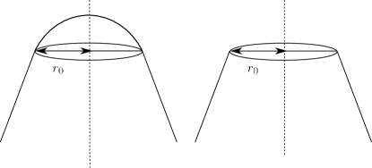
Figure 1: Illustration of the ballpoint pen (left) and flowerpot (right) string geometries.

By the symmetry of the string configuration and vacuum state, the vacuum expectation value of $\phi^{2}$ will depend only on $r$, and we can write the energy density as

$$\langle T_{tt}\rangle=\left\langle\frac{1}{2}(\partial_{t}\phi)^{2}+\frac{1}{2r^{2}}({\cal D}_{r}\phi)^{2}+\frac{1}{2r^{2}}(\partial_{\theta}\phi)^{2}+\frac{\xi}{2}{\cal R}\phi^{2}-\frac{\xi}{r^{2}}{\cal D}_{r}^{2}(\phi^{2})\right\rangle\,,$$ (9)

where $\phi$ obeys the equation of motion

$$\left(\frac{\partial^{2}}{\partial t^{2}}-\frac{1}{r^{2}}{\cal D}_{r}^{2}-\frac{1}{r^{2}}\frac{\partial^{2}}{\partial\theta^{2}}+\xi{\cal R}\right)\phi=0\,.$$ (10)

Again by symmetry, we have $\displaystyle\frac{1}{2}\partial_{t}^{2}\langle\phi^{2}\rangle=\partial_{t}\langle\phi(\partial_{t}\phi)\rangle=0$, and so $\langle\phi(\partial_{t}^{2}\phi)\rangle=-\langle(\partial_{t}\phi)^{2}\rangle$, and similarly for $\theta$. Using these results and $\displaystyle{\cal D}_{r}^{2}(\phi^{2})=2({\cal D}_{r}\phi)^{2}+2\phi{\cal D}_{r}^{2}\phi$, together with the equation of motion, we obtain

$$\left\langle\frac{1}{4r^{2}}{\cal D}_{r}^{2}(\phi^{2})\right\rangle=\left\langle\frac{1}{2r^{2}}({\cal D}_{r}\phi)^{2}-\frac{1}{2}(\partial_{t}\phi)^{2}+\frac{1}{2r^{2}}(\partial_{\theta}\phi)^{2}+\frac{\xi}{2}{\cal R}\phi^{2}\right\rangle\,,$$ (11)

yielding a simplified expression in terms of a consolidated derivative term,

$$\langle T_{tt}\rangle=\left\langle(\partial_{t}\phi)^{2}+\left(\frac{1}{4}-\xi\right)\frac{1}{r^{2}}{\cal D}_{r}^{2}(\phi^{2})\right\rangle\,.$$ (12)

This form will be more convenient for organizing the calculation, particularly with regard to renormalization using the techniques of Ref. [19], but for numerical calculation we will find it preferable to re-expand the second derivative in terms of squared first derivatives.

Our primary tool will be the Green’s function $G_{\sigma}(\bm{r},\bm{r}^{\prime},\kappa)$ for imaginary wave number $k=i\kappa$, which obeys

$$-\left(\frac{1}{r^{2}}{\cal D}_{r}^{2}+\frac{1}{r^{2}}\frac{\partial^{2}}{\partial\theta^{2}}-\xi{\cal R}-\kappa^{2}\right)G_{\sigma}(\bm{r},\bm{r}^{\prime},\kappa)=\frac{1}{rp(r)}\delta(r-r^{\prime})\delta(\theta-\theta^{\prime})\,.$$ (13)

We consider two profile functions [13, 14, 15]: the “flowerpot,”

$$p^{\rm flower}(r)=\begin{cases}\frac{1}{\sigma}&r<r_{0}\\ 1&r>r_{0}\end{cases}$$ (14)

and the “ballpoint pen,”

$$p^{\rm pen}(r)=\begin{cases}\left[\sigma^{2}-\frac{r^{2}}{r_{0}^{2}}(\sigma^{2}-1)\right]^{-1/2}&r<r_{0}\\ 1&r>r_{0}\end{cases}$$ (15)

where $r_{0}$ is the string radius, as shown in Fig. 1. The flowerpot has zero curvature everywhere except for a $\delta$-function contribution at the string radius, while the ballpoint pen has constant curvature $\displaystyle{\cal R}=\frac{2(\sigma^{2}-1)}{r_{0}^{2}}$ inside and zero curvature outside. We write the Green’s function in the scattering form

$$G_{\sigma}(\bm{r},\bm{r}^{\prime},\kappa)=\frac{\sigma}{\pi}\sum_{\ell=0}^{\infty}{}^{\prime}\psi_{\kappa,\ell}^{\rm reg}(r_{<})\psi_{\kappa,\ell}^{\rm out}(r_{>})\cos\left[\sigma\ell(\theta-\theta^{\prime})\right]$$ (16)

where the prime on the sum indicates that the $\ell=0$ term is counted with a weight of one-half, arising because we have written the sum over nonnegative $\ell$ only. The radial wavefunctions obey the equation

$$\left[-\frac{1}{r^{2}}{\cal D}_{r}^{2}+\frac{\ell^{2}\sigma^{2}}{r^{2}}+\xi{\cal R}+\kappa^{2}\right]\psi_{\kappa,\ell}(r)=0\,,$$ (17)

where the regular solution is defined to be well-behaved at $r=0$, while the outgoing solution obeys outgoing wave boundary conditions for $r\to\infty$, normalized to unit amplitude, and $r_{<}$ ($r_{>}$) is the smaller (larger) axial radius of $\bm{r}$ and $\bm{r}^{\prime}$. The functions are normalized so that they obey the Wronskian relation

$$\frac{d}{dr}\left(\psi_{\kappa,\ell}^{\rm reg}(r)\right)\psi_{\kappa,\ell}^{\rm out}(r)-\psi_{\kappa,\ell}^{\rm reg}(r)\frac{d}{dr}\left(\psi_{\kappa,\ell}^{\rm out}(r)\right)=\frac{p(r)}{r}\,,$$ (18)

which provides the appropriate jump condition for the Green’s function.

As shown in Ref. [19], the renormalized energy density of a scalar field in flat spacetime with a background potential that is spherically symmetric in $m$ dimensions and independent of $n$ dimensions after a single “tadpole” subtraction can be written as

$$\langle{\cal H}\rangle_{\rm ren} = -\frac{1}{2(4\pi)^{\frac{n+1}{2}}\Gamma\left(\frac{n+3}{2}\right)}\sum_{\ell=0}^{\infty}D^{m}_{\ell}\int_{0}^{\infty}d\kappa\,2\kappa^{n+2}\left[{\cal G}_{\ell,m}(r,r,\kappa)-{\cal G}_{\ell,m}^{\rm free}(r,r,\kappa)\phantom{\frac{1}{1}}\right.$$ (20)

$$\left.\times\left(1-(2-m)\frac{V_{\ell}(r)}{2\kappa^{2}}\right)-\frac{n+1}{\kappa^{2}}\left(\frac{1}{4}-\xi\right)\frac{1}{r^{2m-2}}{\cal D}^{2}_{r,m}{\cal G}_{\ell,m}(r,r,\kappa)\right]\,,$$

where we have included the contribution from the curvature coupling $\xi$, which contributes to Eq. (3) even when ${\cal R}=0$. Here $\displaystyle\frac{1}{r^{2m-2}}{\cal D}^{2}_{r,m}$ with $\displaystyle{\cal D}_{r,m}=\frac{r^{m-1}}{p(r)}\frac{\partial}{\partial r}$ is the radial Laplacian in $m$ dimensions, $V_{\ell}(r)$ is the scattering potential in channel $\ell$ with degeneracy factor $D^{m}_{\ell}$, and we have decomposed the $m$-dimensional Green’s function for equal angles into its component ${\cal G}_{\ell,m}(r,r^{\prime},\kappa)$ in each channel, which obeys the equation

$$\left(-{\cal D}_{r,m}^{2}+V_{\ell}(r)+\frac{\ell(\ell+m-2)}{r^{2}}+\kappa^{2}\right){\cal G}_{\ell,m}(r,r^{\prime},\kappa)=\delta^{(m)}(r-r^{\prime})$$ (21)

in terms of the $m$-dimensional $\delta$-function. We will focus on the case of $m=2$ and $n=0$, so a single subtraction will be sufficient. The case of a three-dimensional string with $m=2$ and $n=1$ works similarly, but requires additional renormalization counterterms due to the higher degree of divergence.

III Point String and Kontorovich-Lebedev Approach

We begin by reviewing the case of the “point string,” [10, 11, 12] where the radius $r_{0}$ of the string core is taken to zero. The scattering solutions can be obtained using the same techniques as for a conducting wedge [20, 21], but with periodic rather than perfectly reflecting boundary conditions. The normalized scattering functions are $\psi_{\kappa,\ell}^{\rm reg,point}(r)=I_{\sigma\ell}\left(\kappa r\right)$ and $\psi_{\kappa,\ell}^{\rm out,point}(r)=K_{\sigma\ell}\left(\kappa r\right)$, and the Green’s function becomes

$$G_{\sigma}^{\rm point}(\bm{r},\bm{r}^{\prime},\kappa)=\frac{\sigma}{\pi}\sum_{\ell=0}^{\infty}{}^{\prime}I_{\sigma\ell}\left(\kappa r_{<}\right)K_{\sigma\ell}\left(\kappa r_{>}\right)\cos\left[\ell\sigma(\theta-\theta^{\prime})\right]\,,$$ (22)

Setting $\sigma=1$, we obtain the free Green’s function

$$G^{\rm free}(\bm{r},\bm{r}^{\prime},\kappa)=\frac{1}{\pi}\sum_{\ell=0}^{\infty}{}^{\prime}I_{\ell}\left((\kappa r_{<}\right)K_{\ell}\left(\kappa r_{>}\right)\cos\left[\ell(\theta-\theta^{\prime})\right]=\frac{1}{2\pi}K_{0}\left(\kappa\left|re^{i\theta}-r^{\prime}e^{i\theta^{\prime}}\right|\right)\,.$$ (23)

A useful computational tool is to replace the sum over the angular quantum number $\ell$ by a contour integral, based on the Kontorovich-Lebedev transformation. In this approach [22, 23, 24], one multiplies the summand by $\displaystyle\frac{\pi(-1)^{\ell}}{\sin\pi\ell}$, which has poles of unit residue at all integers $\ell$. Because the summand has no other poles in the right half of the complex plane, the original sum over nonnegative $\ell$ then equals the integral of this product over a contour that goes down the imaginary axis and returns by a large semicircle at infinity, taking into account the factor of $2\pi i$ from Cauchy’s theorem. The infinitesimal semicircle needed to go around the pole at $\ell=0$ accounts for the factor of one-half associated with that term in the sum. For the functions we consider, the integral over the large semicircle vanishes, while the contributions from the negative and positive imaginary axis can be folded into a single integral, which often can be simplified through identities such as

$$K_{\nu}(x)=\frac{\pi}{2}\frac{I_{-\nu}(x)-I_{\nu}(x)}{\sin{\nu\pi}}\,,$$ (24)

which is valid for any $\nu$ that is not a real integer.

We illustrate this approach using the point string. To compute finite quantum corrections, we will want to take the difference between the full Green’s function in Eq. (22) and the free Green’s function in Eq. (23), in the limit where the points become coincident, meaning that the individual Green’s functions diverge. However, the necessary cancellation does not emerge term-by-term in the sum, and as a result the standard calculations for this case [10, 15, 21] first carry out the integral over $\kappa$, taking advantage of the availability of analytic results in three space dimensions, which do not exist in our case.

In contrast, using the Kontorovich-Lebedev approach as described above, we obtain

$$G^{\rm free}(\bm{r},\bm{r}^{\prime},\kappa)=\frac{1}{\pi^{2}}\int_{0}^{\infty}d\lambda K_{i\lambda}(\kappa r)K_{i\lambda}(\kappa r^{\prime})\cosh[\lambda(\pi-|\theta-\theta^{\prime}|)]\,,$$ (25)

where we have used $\ell=i\lambda$ and the $\pi$ term in the hyperbolic cosine reflects the $(-1)^{\ell}$ factor above. Note that the jump condition now emerges from the angular rather than the radial component. Similarly, by letting $\sigma\ell=i\lambda$, we obtain for the point string

$$G_{\sigma}^{\rm point}(\bm{r},\bm{r}^{\prime},\kappa)=\frac{1}{\pi^{2}}\int_{0}^{\infty}d\lambda K_{i\lambda}(\kappa r)K_{i\lambda}(\kappa r^{\prime})\cosh\left[\lambda\left(\frac{\pi}{\sigma}-|\theta-\theta^{\prime}|\right)\right]\frac{\sinh\lambda\pi}{\sinh\frac{\lambda}{\sigma}\pi}\,,$$ (26)

and the difference between Green’s functions can be computed by subtraction under the integral sign, yielding after simplification

$$\Delta G_{\sigma}^{\rm point}(r,r,\kappa)=G_{\sigma}^{\rm point}(r,r,\kappa)-G^{\rm free}(r,r,\kappa)=\frac{1}{\pi^{2}}\int_{0}^{\infty}d\lambda K_{i\lambda}(\kappa r)K_{i\lambda}(\kappa r)\frac{\sinh\left[\frac{\lambda}{\sigma}\pi(\sigma-1)\right]}{\sinh\frac{\lambda}{\sigma}\pi}\,,$$ (27)

where we have now taken the limit of coincident points since the difference of Green’s functions is nonsingular.

IV Scattering Wavefunctions

Following Ref. [15], we next compute the regular and outgoing scattering wavefunctions for both the flowerpot and ballpoint pen, each of which will be computed piecewise, with separate expressions inside and outside of the string. In regions where $p(r)$ is constant, namely for $r>r_{0}$ in both models and $r<r_{0}$ for the flowerpot, we have ${\cal R}=0$ and the solutions to Eq. (17) are modified Bessel functions $I_{\tilde{\sigma}\ell}(\kappa r_{*})$ and $K_{\tilde{\sigma}\ell}(\kappa r_{*})$, where $\ell$ is an integer, $\tilde{\sigma}=\sigma p(r)$, and $r_{*}=p(r)r$ is the physical radial distance. For $r<r_{0}$ in the ballpoint pen model, the solutions are Legendre functions $P_{\nu(\kappa)}^{\ell}\left(\tfrac{1}{\sigma p(r)}\right)$ and $Q_{\nu(\kappa)}^{\ell}\left(\tfrac{1}{\sigma p(r)}\right)$ with $\nu(\kappa)(\nu(\kappa)+1)=-\left(\frac{r_{0}^{2}\kappa^{2}}{\sigma^{2}-1}+2\xi\right)$, so that

$$\nu(\kappa)=-\frac{1}{2}+\frac{1}{2}\sqrt{(1-8\xi)-\frac{4\kappa^{2}r_{0}^{2}}{\sigma^{2}-1}}\,.$$ (28)

We can thus write the full solutions as

$$\psi_{\kappa,\ell}^{\rm pen}(r)=\begin{array}[]{|c|c|c|}\hline\cr&r<r_{0}&r>r_{0}\cr\hline\cr\hbox{regular}&A_{\kappa,\ell}^{\rm pen}P_{\nu(\kappa)}^{\ell}\left(\tfrac{1}{\sigma p(r)}\right)&I_{\sigma\ell}(\kappa r)+B_{\kappa,\ell}^{\rm pen}K_{\sigma\ell}(\kappa r)\cr\hline\cr\hbox{outgoing}&C_{\kappa,\ell}^{\rm pen}P_{\nu(\kappa)}^{\ell}\left(\tfrac{1}{\sigma p(r)}\right)+D_{\kappa,\ell}^{\rm pen}Q_{\nu(\kappa)}^{\ell}\left(\tfrac{1}{\sigma p(r)}\right)&K_{\sigma\ell}(\kappa r)\cr\hline\cr\end{array}$$ (29)

for the ballpoint pen and

$$\psi_{\kappa,\ell}^{\rm flower}(r)=\begin{array}[]{|c|c|c|}\hline\cr&r<r_{0}&r>r_{0}\cr\hline\cr\hbox{regular}&A_{\kappa,\ell}^{\rm flower}I_{\ell}\left(\kappa\frac{r}{\sigma}\right)&I_{\sigma\ell}(\kappa r)+B_{\kappa,\ell}^{\rm flower}K_{\sigma\ell}(\kappa r)\cr\hline\cr\hbox{outgoing}&C_{\kappa,\ell}^{\rm flower}I_{\ell}\left(\kappa\frac{r}{\sigma}\right)+D_{\kappa,\ell}^{\rm flower}K_{\ell}\left(\kappa\frac{r}{\sigma}\right)&K_{\sigma\ell}(\kappa r)\cr\hline\cr\end{array}$$ (30)

for the flowerpot. In these expressions, for $r>r_{0}$ the coefficient of the outgoing wave is normalized to one, and then we can also set the coefficient of the first-kind solution in the regular wave to one by the Wronskian relation, Eq. (18). For $r<r_{0}$, the regular solution must be proportional to the the first-kind function, since it is the only solution regular at the origin. In the ballpoint pen model, both the wavefunction and its first derivative are continuous at $r=r_{0}$, while in the flowerpot model the wavefunction and the quantity

$$\frac{r}{p(r)}\frac{d}{dr}\psi_{\kappa,\ell}^{\rm flower}(r)+2\xi\frac{\psi_{\kappa,\ell}^{\rm flower}(r)}{p(r)}$$ (31)

are continuous at $r=r_{0}$ (note that $p(r)$ is discontinuous). The boundary conditions for the function and its first derivative at $r=r_{0}$ thus yield four equations for the four unknown coefficients. In addition, from the Wronskian relation for $r<r_{0}$ we know that

$$A_{\kappa,\ell}^{\rm pen}D_{\kappa,\ell}^{\rm pen}=\frac{1}{\sigma}\frac{\Gamma(\nu(\kappa)-\ell+1)}{\Gamma(\nu(\kappa)+\ell+1)}\hbox{\qquad and \qquad}A_{\kappa,\ell}^{\rm flower}D_{\kappa,\ell}^{\rm flower}=\frac{1}{\sigma}\,.$$ (32)

Given this result, for brevity we quote only the remaining combinations we will need to form the Green’s function,

$$\frac{C_{\kappa,\ell}^{\rm pen}}{D_{\kappa,\ell}^{\rm pen}} = -\frac{(\sigma^{2}-1)Q_{\nu(\kappa)}^{\ell}{}^{\prime}\left(\tfrac{1}{\sigma}\right)K_{\sigma\ell}\left(\kappa r_{0}\right)+\sigma\kappa r_{0}Q_{\nu(\kappa)}^{\ell}\left(\tfrac{1}{\sigma}\right)K_{\sigma\ell}^{\prime}\left(\kappa r_{0}\right)}{(\sigma^{2}-1)P_{\nu(\kappa)}^{\ell}{}^{\prime}\left(\tfrac{1}{\sigma}\right)K_{\sigma\ell}\left(\kappa r_{0}\right)+\sigma\kappa r_{0}P_{\nu(\kappa)}^{\ell}\left(\tfrac{1}{\sigma}\right)K_{\sigma\ell}^{\prime}\left(\kappa r_{0}\right)}$$ (33)

$$B_{\kappa,\ell}^{\rm pen} = -\frac{(\sigma^{2}-1)P_{\nu(\kappa)}^{\ell}{}^{\prime}\left(\tfrac{1}{\sigma}\right)I_{\sigma\ell}\left(\kappa r_{0}\right)+\sigma\kappa r_{0}P_{\nu(\kappa)}^{\ell}\left(\tfrac{1}{\sigma}\right)I_{\sigma\ell}^{\prime}\left(\kappa r_{0}\right)}{(\sigma^{2}-1)P_{\nu(\kappa)}^{\ell}{}^{\prime}\left(\tfrac{1}{\sigma}\right)K_{\sigma\ell}\left(\kappa r_{0}\right)+\sigma\kappa r_{0}P_{\nu(\kappa)}^{\ell}\left(\tfrac{1}{\sigma}\right)K_{\sigma\ell}^{\prime}\left(\kappa r_{0}\right)}$$ (34)

and

$$\frac{C_{\kappa,\ell}^{\rm flower}}{D_{\kappa,\ell}^{\rm flower}} = -\frac{K_{\ell}^{\prime}\left(\kappa\frac{r_{0}}{\sigma}\right)K_{\sigma\ell}\left(\kappa r_{0}\right)-K_{\ell}\left(\kappa\frac{r_{0}}{\sigma}\right)K_{\sigma\ell}^{\prime}\left(\kappa r_{0}\right)+\frac{2\xi(\sigma-1)}{\kappa r_{0}}K_{\ell}\left(\kappa\frac{r_{0}}{\sigma}\right)K_{\sigma\ell}\left(\kappa r_{0}\right)}{I_{\ell}^{\prime}\left(\kappa\frac{r_{0}}{\sigma}\right)K_{\sigma\ell}\left(\kappa r_{0}\right)-I_{\ell}\left(\kappa\frac{r_{0}}{\sigma}\right)K_{\sigma\ell}^{\prime}\left(\kappa r_{0}\right)+\frac{2\xi(\sigma-1)}{\kappa r_{0}}I_{\ell}\left(\kappa\frac{r_{0}}{\sigma}\right)K_{\sigma\ell}\left(\kappa r_{0}\right)}$$ (35)

$$B_{\kappa,\ell}^{\rm flower} = -\frac{I_{\ell}^{\prime}\left(\kappa\frac{r_{0}}{\sigma}\right)I_{\sigma\ell}\left(\kappa r_{0}\right)-I_{\ell}\left(\kappa\frac{r_{0}}{\sigma}\right)I_{\sigma\ell}^{\prime}\left(\kappa r_{0}\right)+\frac{2\xi(\sigma-1)}{\kappa r_{0}}I_{\ell}\left(\kappa\frac{r_{0}}{\sigma}\right)I_{\sigma\ell}\left(\kappa r_{0}\right)}{I_{\ell}^{\prime}\left(\kappa\frac{r_{0}}{\sigma}\right)K_{\sigma\ell}\left(\kappa r_{0}\right)-I_{\ell}\left(\kappa\frac{r_{0}}{\sigma}\right)K_{\sigma\ell}^{\prime}\left(\kappa r_{0}\right)+\frac{2\xi(\sigma-1)}{\kappa r_{0}}I_{\ell}\left(\kappa\frac{r_{0}}{\sigma}\right)K_{\sigma\ell}\left(\kappa r_{0}\right)}\,,$$ (36)

where prime denotes a derivative with respect to the function’s argument.

Finally, we note that when $\ell$ is not a real integer, as will arise in situations we consider below, for $r<r_{0}$ it is computationally preferable to take as independent solutions $P_{\nu(\kappa)}^{\ell}$ and $P_{\nu(\kappa)}^{-\ell}$ rather than $P_{\nu(\kappa)}^{\ell}$ and $Q_{\nu(\kappa)}^{\ell}$ for the ballpoint pen, and $I_{\ell}$ and $I_{-\ell}$ rather than $I_{\ell}$ and $K_{\ell}$ for the flowerpot. With these replacements made throughout, the same formulae hold as above, except that the right-hand side of Eq. (32) becomes $\displaystyle\frac{\pi}{2\sigma\sin\pi\ell}$ in both cases.

V Renormalization: Free Green’s Function Subtraction

In regions where $p(r)$ is constant, we have a flat spacetime (although possibly with a deficit angle), and so to obtain renormalized quantities we must only subtract the contribution of the free Green’s function. As in the case of the point string, however, the necessary cancellation may not appear term by term in the sum over $\ell$, making numerical calculations difficult.

For $r>r_{0}$, we again use the approach of Ref. [15] and consider the difference between the full string and a point string with the same $\sigma$. We can then add the difference between the point string and empty space using Eq. (27). We obtain, in both models,

$$G_{\sigma}(\bm{r},\bm{r}^{\prime},\kappa)-G_{\sigma}^{\rm point}(\bm{r},\bm{r}^{\prime},\kappa)=\frac{\sigma}{\pi}\sum_{\ell=0}^{\infty}{}^{\prime}B_{\kappa,\ell}K_{\sigma\ell}\left(\kappa r\right)K_{\sigma\ell}\left(\kappa r^{\prime}\right)\cos\left[\ell(\theta-\theta^{\prime})\right]$$ (37)

for $r,r^{\prime}>r_{0}$, written in terms of the scattering coefficient described above for each model. For the flowerpot model with $r<r_{0}$, we also have flat space, although now corresponding to zero interior deficit angle $\tilde{\sigma}=p(r)\sigma=1$, and with the physical distance to the origin given by $\displaystyle r_{*}=\frac{r}{\sigma}$. We can therefore subtract the free Green’s function directly, evaluating it the same physical distances,

$$G_{\sigma}^{\rm flower}(\bm{r},\bm{r}^{\prime},\kappa)-G^{\rm free}(\bm{r}_{*},\bm{r}^{\prime}_{*},\kappa)=\frac{1}{\pi}\sum_{\ell=0}^{\infty}{}^{\prime}\frac{C_{\kappa,\ell}^{\rm flower}}{D_{\kappa,\ell}^{\rm flower}}I_{\sigma\ell}\left(\kappa r\right)I_{\sigma\ell}\left(\kappa r^{\prime}\right)\cos\left[\ell(\theta-\theta^{\prime})\right]\,.$$ (38)

We can evaluate these expressions at coincident points, since the singularity cancels through the subtraction.

For $r<r_{0}$ in the ballpoint pen model, we will use a hybrid of these subtractions. First, we define

$$r_{*}=\frac{r_{0}}{\sqrt{\sigma^{2}-1}}\arccos\frac{1}{\sigma p(r)}\qquad\Leftrightarrow\qquad r=\frac{r_{0}\sigma}{\sqrt{\sigma^{2}-1}}\sin\frac{r_{*}\sqrt{\sigma^{2}-1}}{r_{0}}$$ (39)

so that $\displaystyle\frac{dr_{*}}{dr}=p(r)$ and $r_{*}$ represents the physical distance to the origin. We then subtract the contribution from a point string with deficit angle $\tilde{\sigma}=\sigma p(r)$, corresponding to the angle deficit at that point, evaluated at $r_{*}$. As above, we add back in the contribution of this point string using the results of the previous section.

There is one further subtlety in this calculation. The free Green’s function, what we ultimately subtract, depends only on the separation between points, and thus is unchanged by translation or rescaling. However, to carry out the subtraction, we must separate the points by a distance $\epsilon$ in both Green’s functions, and then take the limit of the difference as $\epsilon$ goes to zero. The limit should correspond to splitting the points by the same physical distance. Since

$$\lim_{\epsilon\to 0}\left[K_{0}(a\epsilon)-K_{0}(\epsilon)\right]=-\log a\,,$$ (40)

we therefore must subtract $\displaystyle\frac{1}{2\pi}\log\frac{r_{*}}{rp(r)}$ to correct for this discrepancy.

Thus we obtain, for $r<r_{0}$,

$$G_{\sigma}^{\rm pen}(r,r,\kappa)-G_{\tilde{\sigma}}^{\rm point}(r_{*},r_{*},\kappa) = \frac{1}{\pi}\sum_{\ell=0}^{\infty}{}^{\prime}\Bigg{[}\frac{\Gamma(\nu(\kappa)-\ell+1)}{\Gamma(\nu(\kappa)+\ell+1)}P_{\nu(\kappa)}^{\ell}\left(\tfrac{1}{\sigma p(r)}\right)\left(\frac{C_{\kappa,\ell}^{\rm pen}}{D_{\kappa,\ell}^{\rm pen}}P_{\nu(\kappa)}^{\ell}\left(\tfrac{1}{\sigma p(r)}\right)+Q_{\nu(\kappa)}^{\ell}\left(\tfrac{1}{\sigma p(r)}\right)\right)$$ (42)

$$-\tilde{\sigma}I_{\tilde{\sigma}\ell}\left(\kappa r_{*}\right)K_{\tilde{\sigma}\ell}\left(\kappa r_{*}\right)\Bigg{]}-\frac{1}{2\pi}\log\frac{r_{*}}{rp(r)}$$

in the limit of coincident points.

VI Renormalization: Tadpole Subtraction

In the case of the ballpoint pen for $r<r_{0}$, the string background effectively creates a background potential, leading to additional counterterms. Following Ref. [19], we use dimensional regularization and consider configurations that are trivial in $n$ dimensions and spherically symmetric in $m$ dimensions, meaning that a string in three space dimensions corresponds to the case of $n=1$, $m=2$. After integrating over the $n$ trivial directions, the contribution ${\cal G}_{\ell}(r,r^{\prime},\kappa)$ to the Green’s function from angular momentum channel $\ell$ in $m$ dimensions is replaced by the subtracted quantity

$${\cal G}_{\ell,m}(r,r,\kappa)-{\cal G}^{\rm free}_{\ell,m}(r,r,\kappa)+(2-m)\frac{V_{\ell}(r)}{2\kappa^{2}}{\cal G}^{\rm free}_{\ell,m}(r,r,\kappa)$$ (43)

where $V_{\ell}(r)$ is the background potential for that channel. Here the first subtraction represents the free background and the second represents the tadpole graph. Since we are interested in $m=2$, the latter contribution appears to vanish. However, it multiplies the free Green’s function at coincident points, which diverges, so we must take the limit carefully. To do so, we consider the free radial Green’s function in $m$ dimensions for channel $\ell$,

$${\cal G}^{\rm free}_{\ell,m}(r,r^{\prime},\kappa)=\frac{\Gamma\left(\frac{m}{2}\right)}{2\pi^{\frac{m}{2}}}\frac{1}{(rr^{\prime})^{\frac{m}{2}-1}}I_{\frac{m}{2}-1+\ell}(\kappa r_{<})K_{\frac{m}{2}-1+\ell}(\kappa r_{>})\,.$$ (44)

Its contribution is weighted by the degeneracy factor

$$D^{m}_{\ell}=\frac{\Gamma(m+\ell-2)}{\Gamma(m-1)\Gamma(\ell+1)}(m+2\ell-2)\,,$$ (45)

which has the following limits as special cases

$$D^{m=2}_{\ell}=2-\delta_{\ell 0}\qquad D^{m=1}_{\ell}=\delta_{\ell 0}+\delta_{\ell 1}\qquad D^{m=0}_{\ell}=\delta_{\ell 0}\,,$$ (46)

expressed in terms of the Kronecker $\delta$ symbol. For equal angles, the free Green’s function is then given by the sum

$$G^{\rm free}_{m}(r,r^{\prime},\kappa)=\frac{1}{(2\pi)^{\frac{m}{2}}}\left(\frac{\kappa}{|r-r^{\prime}|}\right)^{\frac{m}{2}-1}K_{\frac{m}{2}-1}(\kappa|r-r^{\prime}|)=\sum_{\ell=0}^{\infty}D^{m}_{\ell}{\cal G}^{\rm free}_{\ell,m}(r,r^{\prime},\kappa)\,.$$ (47)

To bring the points together, we expand around $r=r^{\prime}=0$ (since the free Green’s function only depends on their difference, we may choose to have them both approach any point we choose), in which case we have

$$(2-m)D^{m}_{\ell}{\cal G}^{\rm free}_{\ell,m}(r,r,\kappa)=-(2-m)\left[\left(\frac{\kappa r}{2}\right)^{2\ell}\frac{\kappa^{m-2}\left(m+2\ell\right)\Gamma\left(\frac{m}{2}\right)\Gamma\left(2-\frac{m}{2}-\ell\right)\Gamma(m+\ell-2)}{(4\pi)^{\frac{m}{2}}\Gamma(m-1)\Gamma(\ell+1)\Gamma\left(1+\frac{m}{2}+\ell\right)}+{\cal O}(r^{2-m})\right]\,,$$ (48)

where, crucially, we have dropped terms of order $r^{2-m}$ because we approach $m=2$ from below, where the integrals converge, and so these terms vanish for $r\to 0$. When $\ell\neq 0$, the term we have kept also vanishes for $r\to 0$. However, for $\ell=0$, it goes to $\displaystyle\frac{1}{2\pi}$ in the limit $m\to 2$, and so we have found

$$\lim_{m\to 2}\left[(2-m)D^{m}_{\ell}{\cal G}^{\rm free}_{\ell,m}(r=0,r=0,\kappa)\right]=\frac{1}{2\pi}\delta_{\ell 0}\quad\Longrightarrow\quad\lim_{m\to 2}\left[(2-m)\sum_{\ell=0}^{\infty}D^{m}_{\ell}{\cal G}^{\rm free}_{\ell,m}(r,r,\kappa)V_{\ell}(r)\right]=\frac{1}{2\pi}V_{\ell=0}(r)\,,$$ (49)

with the result for the summed Green’s function depending only on the contribution of the potential in the $\ell=0$ channel.

To find the potential $V_{\ell}(r)$, we rewrite the wave equation for $r<r_{0}$ using the physical radius $r_{*}$ given in Eq. (39). The rescaled wavefunction $\displaystyle\phi_{\kappa,\ell}(r_{*})=\sqrt{r}\psi_{\kappa,\ell}(r)$ then obeys [25]

$$\left[-\frac{d^{2}}{dr_{*}^{2}}+\sigma^{2}\left(\frac{\ell^{2}-\frac{1}{4}}{r^{2}}\right)-\frac{1}{4}\left(\frac{\sigma^{2}-1}{r_{0}^{2}}\right)+\xi{\cal R}+\kappa^{2}\right]\phi_{\kappa,\ell}(r_{*})=0\,,$$ (50)

where the denominator of the second term represents $r$ as a function of $r_{*}$. A free particle would instead obey the equation

$$\left[-\frac{d^{2}}{dr_{*}^{2}}+\left(\frac{\ell^{2}-\frac{1}{4}}{r_{*}^{2}}\right)+\kappa^{2}\right]\phi^{\rm free}_{\kappa,\ell}(r_{*})=0\,,$$ (51)

and so we can consider the difference between the two expressions in brackets as a scattering potential,

$$V_{\ell}^{\rm full}(r)=\frac{\left(\ell^{2}-\frac{1}{4}\right)\sigma^{2}}{r^{2}}-\frac{\left(\ell^{2}-\frac{1}{4}\right)\left(\sigma^{2}-1\right)}{r_{0}^{2}\left(\arccos\frac{1}{\sigma p(r)}\right)^{2}}+\frac{(8\xi-1)\left(\sigma^{2}-1\right)}{4r_{0}^{2}}\,.$$ (52)

For the counterterm, we need only the $\ell=0$ case, and the tadpole subtraction is given by the leading order in perturbation theory. We take $\sigma^{2}-1$ as the coupling constant. Expanding to leading order in this quantity, we obtain the tadpole contribution for $r<r_{0}$,

$$V_{\ell=0}(r)=2\frac{\sigma^{2}-1}{r_{0}^{2}}\left(\xi-\frac{1}{6}\right)={\cal R}\left(\xi-\frac{1}{6}\right)\,,$$ (53)

which is independent of $r$ and vanishes for conformal coupling in three dimensions. Note that this term exactly coincides with the first-order heat kernel coefficient [26].

Putting these results together, we obtain the subtracted Green’s function summed over angular momentum channels

$$G_{\sigma}(r,r,\kappa)-G^{\rm free}(r,r,\kappa)+\frac{V_{\ell=0}(r)}{4\pi\kappa^{2}}=G_{\sigma}(r,r,\kappa)-G^{\rm free}(r,r,\kappa)+\frac{{\cal R}}{4\pi\kappa^{2}}\left(\xi-\frac{1}{6}\right)$$ (54)

in the limit where $m\to 2$ and the points are coincident. Furthermore, we can pull the last term of Eq. (54) inside the sum used to define the Green’s function by using a special case of the addition theorem for Legendre functions,

$$1=2\sum_{\ell=0}^{\infty}{}^{\prime}\frac{\Gamma(\nu(\kappa)-\ell+1)}{\Gamma(\nu(\kappa)+\ell+1)}P_{\nu(\kappa)}^{\ell}\left(\tfrac{1}{\sigma p(r)}\right)^{2}\,.$$ (55)

VII Derivative Term

Next we compute the derivative term $\displaystyle\frac{1}{r^{2}}{\cal D}_{r}^{2}G_{\sigma}(\bm{r},\bm{r},\kappa)$ by differentiating the expressions above. We note that for any two functions of $\psi_{A}(r)$ and $\psi_{B}(r)$,

$${\cal D}_{r}^{2}(\psi_{A}(r)\psi_{B}(r))=2({\cal D}_{r}\psi_{A}(r))({\cal D}_{r}\phi_{B}(r))+\psi_{A}(r)\left({\cal D}_{r}^{2}\psi_{B}(r)\right)+\left({\cal D}_{r}^{2}\psi_{A}(r)\right)\psi_{B}(r)\,,$$ (56)

and so by using the equations of motion, we can express the terms involving squares of first derivatives in terms of the second derivative of the product, and vice versa. Accordingly, for any pair of solutions $\psi_{A}(r)$ and $\psi_{B}(r)$ obeying Eq. (17), we have

$$\frac{1}{2r^{2}}{\cal D}_{r}^{2}\left(\psi_{\kappa,\ell}^{A}(r)\psi_{\kappa,\ell}^{B}(r)\right)=\left(\frac{(\sigma\ell)^{2}}{r^{2}}+\xi{\cal R}+\kappa^{2}\right)\psi_{\kappa,\ell}^{A}(r)\psi_{\kappa,\ell}^{B}(r)+\frac{1}{r^{2}}\left({\cal D}_{r}\psi_{\kappa,\ell}^{A}(r)\right)\left({\cal D}_{r}\psi_{\kappa,\ell}^{B}(r)\right)\,,$$ (57)

and we note that

$$\frac{1}{p(r)}\frac{d}{dr}P_{\nu(\kappa)}^{\ell}\left(\tfrac{1}{\sigma p(r)}\right)=-\frac{r(\sigma^{2}-1)}{r_{0}^{2}\sigma}P_{\nu(\kappa)}^{\ell}{}^{\prime}\left(\tfrac{1}{\sigma p(r)}\right)\,,$$ (58)

and similarly for $Q_{\nu(\kappa)}^{\ell}$, and so by using recurrence relations we can simplify

$$\frac{1}{2r^{2}}{\cal D}_{r}^{2}\left[P_{\nu(\kappa)}^{\ell}\left(\tfrac{1}{\sigma p(r)}\right)Z_{\nu(\kappa)}^{\ell}\left(\tfrac{1}{\sigma p(r)}\right)\right] = \left(\frac{(\sigma\ell)^{2}}{r^{2}}+\xi{\cal R}+\kappa^{2}\right)P_{\nu(\kappa)}^{\ell}\left(\tfrac{1}{\sigma p(r)}\right)Z_{\nu(\kappa)}^{\ell}\left(\tfrac{1}{\sigma p(r)}\right)$$ (61)

$$+\frac{1}{r^{2}}\left[\frac{r\sqrt{\sigma^{2}-1}}{r_{0}}P_{\nu(\kappa)}^{\ell+1}\left(\tfrac{1}{\sigma p(r)}\right)+\frac{\ell}{p(r)}P_{\nu(\kappa)}^{\ell}\left(\tfrac{1}{\sigma p(r)}\right)\right]$$

$$\times\left[\frac{r\sqrt{\sigma^{2}-1}}{r_{0}}Z_{\nu(\kappa)}^{\ell+1}\left(\tfrac{1}{\sigma p(r)}\right)+\frac{\ell}{p(r)}Z_{\nu(\kappa)}^{\ell}\left(\tfrac{1}{\sigma p(r)}\right)\right]$$

where $Z$ is either $P$ or $Q$; similar simplifications based on recurrence relations apply for Bessel functions.

Renormalization of the derivative term in the curved space background requires an additional counterterm compared to the flat space expression in Eq. (20). This subtraction is also proportional to the curvature scalar ${\cal R}$. The renormalized derivative term becomes

$$\frac{1}{r^{2}}{\cal D}_{r}^{2}G_{\sigma}(r,r,\kappa)-\frac{1}{4\pi}{\cal R}\,,$$ (62)

where again the counterterm is proportional to the Ricci scalar and we have taken the points to be coincident. With this choice, the full tadpole counterterm contribution to the modified integrand of Eq. (20) with $m=2$ and $n=0$ is

$$\kappa^{2}\frac{{\cal R}}{4\pi\kappa^{2}}\left(\xi-\frac{1}{6}\right)+\left(\frac{1}{4}-\xi\right)\frac{{\cal R}}{4\pi}=\frac{{\cal R}}{48\pi}\,,$$ (63)

consistent with the general result originating from the two-dimensional conformal anomaly [27, 28, 29], since our geometry is only curved in two dimensions. As above, we can pull this term inside the sum using Eq. (55).

Finally, as before we find it more computationally tractable to compute the derivative term for the difference of the full Green’s function and the corresponding point string. We must then add back the derivative of the point string contribution as well. In both what we subtract and add back in, we define the radial derivative for the point string contribution taking $p(r)$ constant, corresponding to the derivative we would use in the point string case.

VIII Kontorovich-Lebedev Approach for Nonzero Width String

As with the point string above, we can express the Green’s function as an integral over imaginary angular momentum $\lambda$ using the Kontorovich-Lebedev approach. As described above, we take the pairs $P_{\nu(\kappa)}^{\ell}$ and $P_{\nu(\kappa)}^{-\ell}$ and $I_{\ell}$ and $I_{-\ell}$ as the independent solutions for $r<r_{0}$ in the ballpoint pen and flowerpot models respectively.

The Green’s function becomes

$$G_{\sigma}(\bm{r},\bm{r}^{\prime},\kappa)=\frac{1}{2\pi}\int_{0}^{\infty}\frac{id\lambda}{\sinh\frac{\lambda\pi}{\sigma}}\left[\psi_{\kappa,i\frac{\lambda}{\sigma}}^{\rm reg}(r_{<})-\psi_{\kappa,-i\frac{\lambda}{\sigma}}^{\rm reg}(r_{<})\right]\psi_{\kappa,i\frac{\lambda}{\sigma}}^{\rm out}(r_{>})\cosh\left[\lambda\left(\frac{\pi}{\sigma}-|\theta-\theta^{\prime}|\right)\right]\,,$$ (64)

where we have used that the outgoing wave is always even in $\lambda$. For $r>r_{0}$, we can use Wronskian relationships to simplify

$$\frac{i}{\sinh\frac{\lambda\pi}{\sigma}}\left[\psi_{\kappa,i\frac{\lambda}{\sigma}}^{\rm reg,pen}(r)-\psi_{\kappa,-i\frac{\lambda}{\sigma}}^{\rm reg,pen}(r)\right]=\frac{\frac{2}{\pi}\sigma^{3}K_{i\lambda}\left(\kappa r\right)}{|(\sigma^{2}-1)P_{\nu(\kappa)}^{i\frac{\lambda}{\sigma}}{}^{\prime}\left(\tfrac{1}{\sigma}\right)K_{i\lambda}\left(\kappa r_{0}\right)+\sigma\kappa r_{0}P_{\nu(\kappa)}^{i\frac{\lambda}{\sigma}}\left(\tfrac{1}{\sigma}\right)K_{i\lambda}^{\prime}\left(\kappa r_{0}\right)|^{2}}$$ (65)

for the ballpoint pen and

$$\frac{i}{\sinh\frac{\lambda\pi}{\sigma}}\left[\psi_{\kappa,i\frac{\lambda}{\sigma}}^{\rm reg,flower}(r)-\psi_{\kappa,-i\frac{\lambda}{\sigma}}^{\rm reg,flower}(r)\right]=\frac{\frac{2}{\pi}\frac{\sigma}{\kappa^{2}r_{0}^{2}}K_{i\lambda}\left(\kappa r\right)}{|I_{i\frac{\lambda}{\sigma}}^{\prime}\left(\kappa\frac{r_{0}}{\sigma}\right)K_{i\lambda}\left(\kappa r_{0}\right)-I_{i\frac{\lambda}{\sigma}}\left(\kappa\frac{r_{0}}{\sigma}\right)K_{i\lambda}^{\prime}\left(\kappa r_{0}\right)+\frac{2\xi(\sigma-1)}{\kappa r_{0}}I_{i\frac{\lambda}{\sigma}}\left(\kappa\frac{r_{0}}{\sigma}\right)K_{i\lambda}\left(\kappa r_{0}\right)|^{2}}$$ (66)

for the flowerpot. For $r<r_{0}$, we have

$$\frac{i}{\sinh\frac{\lambda\pi}{\sigma}}\left[\psi_{\kappa,i\frac{\lambda}{\sigma}}^{\rm reg}(r)-\psi_{\kappa,-i\frac{\lambda}{\sigma}}^{\rm reg}(r)\right]=\frac{i}{\sinh\frac{\lambda\pi}{\sigma}}\frac{A_{\kappa,\frac{i\lambda}{\sigma}}}{C_{\kappa,\frac{i\lambda}{\sigma}}}\psi_{\kappa,i\frac{\lambda}{\sigma}}^{\rm out}(r)\,,$$ (67)

and so in both cases the Green’s function is written entirely in terms of outgoing waves. We can then subtract the free Green’s function in the form of Eq. (25). For numerical calculation, however, we find that this approach is only effective for $r>r_{0}$.

IX Results

Collecting all of these terms, we have the full expression for the renormalized energy density, written with the point string subtracted and then added back in,

$$\langle{\cal H}\rangle_{\rm ren} = -\frac{1}{\pi}\int_{0}^{\infty}d\kappa\Bigg{[}\kappa^{2}\left(G_{\sigma}(r,r,\kappa)-G_{\tilde{\sigma}}^{\rm point}(r_{*},r_{*},\kappa)+\Delta G_{\tilde{\sigma}}^{\rm point}(r_{*},r_{*},\kappa)-\frac{1}{2\pi}\log\frac{r_{*}}{rp(r)}\right)$$ (69)

$$-\left(\frac{1}{4}-\xi\right)\frac{1}{r^{2}}\left({\cal D}_{r}^{2}G_{\sigma}(r,r,\kappa)-\bar{\cal D}_{r}^{2}G_{\tilde{\sigma}}^{\rm point}(r_{*},r_{*},\kappa)+\bar{\cal D}_{r}^{2}\Delta G_{\tilde{\sigma}}^{\rm point}(r_{*},r_{*},\kappa)\right)+\frac{{\cal R}}{48\pi}\Bigg{]}$$

where $r_{*}$ is the physical distance in each model as defined above (with $r_{*}=r$ for $r>r_{0}$) and $\tilde{\sigma}=p(r)\sigma$ in each region (with $\tilde{\sigma}=\sigma$ for $r>r_{0}$). Here we have defined $\displaystyle\bar{\cal D}_{r}=r\frac{d}{dr}$ so that we add and subtract derivatives of the point string in the background of a flat spacetime with a deficit angle, as described above. The combined counterterm $\displaystyle\frac{{\cal R}}{48\pi}$ (with ${\cal R}=0$ for $r>r_{0}$, and for $r<r_{0}$ in the flowerpot model) is obtained by combining the two individual terms obtained in Sec. VI using Eq. (63).

In both the first and second lines of Eq. (69), the contribution from the difference between the full and point string Green’s functions can be taken inside the sum over $\ell$, using the results in Sec. V and Eq. (22), while the contribution from the difference between the point string and empty space Green’s functions can be computed as an integral over imaginary angular momentum using Eq. (27). For the case of $r>r_{0}$, we can check our calculation using the results of Sec. VIII, in which case Eq. (69) can be expressed entirely in terms of an integral on the imaginary angular momentum axis. For that calculation, there is no need to add and subtract the point cone contribution, so we can simply subtract the free Green’s function directly, using Eq. (25).

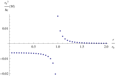
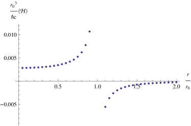
Figure 2: Energy density $\langle\cal H\rangle_{\rm ren}$, in units of $\displaystyle\frac{\hbar c}{r_{0}^{3}}$, as a function of $r$, in units of $r_{0}$, for $\displaystyle\theta_{0}=\frac{\pi}{3}$ in the ballpoint pen model. The left panel shows minimal coupling $\xi=0$, while the right panel shows conformal coupling $\displaystyle\xi=\frac{1}{8}$.

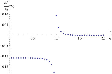
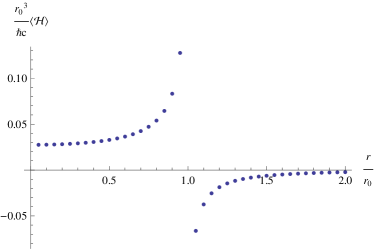
Figure 3: Energy density $\langle\cal H\rangle_{\rm ren}$, in units of $\displaystyle\frac{\hbar c}{r_{0}^{3}}$, as a function of $r$, in units of $r_{0}$, for $\displaystyle\theta_{0}=\frac{2\pi}{3}$ in the ballpoint pen model. The left panel shows minimal coupling $\xi=0$, while the right panel shows conformal coupling $\displaystyle\xi=\frac{1}{8}$. The energy shows a similar shape, but larger magnitude for a greater deficit angle.

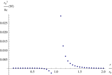
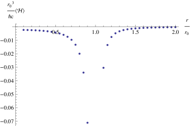
Figure 4: Energy density $\langle\cal H\rangle_{\rm ren}$, in units of $\displaystyle\frac{\hbar c}{r_{0}^{3}}$, as a function of $r$, in units of $r_{0}$, for $\displaystyle\theta_{0}=\frac{\pi}{3}$ in the flowerpot model. The left panel shows minimal coupling $\xi=0$, while the right panel shows conformal coupling $\displaystyle\xi=\frac{1}{8}$. The energy density for minimal coupling is small for $r<r_{0}$ because this case is close to the deficit angle where the inside energy density changes sign.

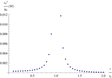
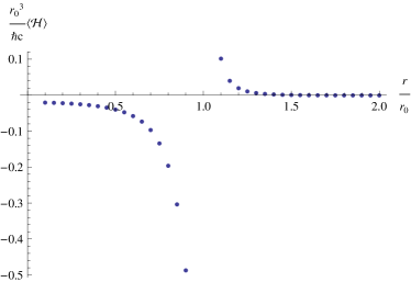
Figure 5: Energy density $\langle\cal H\rangle_{\rm ren}$, in units of $\displaystyle\frac{\hbar c}{r_{0}^{3}}$, as a function of $r$, in units of $r_{0}$, for $\displaystyle\theta_{0}=\frac{\pi}{6}$ (left panel) and $\displaystyle\theta_{0}=\frac{2\pi}{3}$ (right panel in the flowerpot model with $\xi=0$. The sign of the energy density for $r<r_{0}$ reverses at approximately $\theta_{0}\approx 1$.

Sample results are shown in Figs. 2 through 5, for both minimal and conformal coupling. We note that for the interior of the flowerpot, the sign of the energy density for $r<r_{0}$ is opposite at large and small deficit angles for minimal coupling, with the sign change occurring at $\theta_{0}\approx 1$. For the ballpoint pen, we see a discontinuity at $r=r_{0}$, corresponding to the discontinuity in the curvature. For the flowerpot, the energy density diverges at $r=r_{0}$, corresponding to the $\delta$-function curvature profile.

X Conclusions

We have shown how to use scattering data to compute the quantum energy density of a massless scalar field in the background on a nonzero width cosmic string background, using both the “flowerpot” and “ballpoint pen” string profiles in two space dimensions. Of particular interest is the interior of the ballpoint pen, where the background space time has nontrivial (but constant) curvature. We precisely specify counterterms corresponding to renormalization of both the cosmological constant and the gravitational coupling to the scalar curvature ${\cal R}$. In addition, to make the calculation tractable numerically, we subtract and then add back in the contribution of a “point string” with the same deficit angle and physical radius. We can then subtract the free space contribution, corresponding to the cosmological constant renormalization, by combining it with the point string result and using analytic continuation of the angular momentum sum to an integral over the imaginary axis. These results extend straightforwardly to three dimensions, but that case requires an additional subtraction of order ${\cal R}^{2}$.

XI Acknowledgments

It is a pleasure to thank K. Olum for sharing preliminary work on this topic and H. Weigel for helpful conversations and feedback. M. K., X. L., and N. G. were supported in part by the National Science Foundation (NSF) through grant PHY-2205708.

References

Dashen et al. [1974]
R. F. Dashen,
B. Hasslacher,
and A. Neveu,
Phys.Rev. D 10,
4114 (1974).
Rebhan and van Nieuwenhuizen [1997]
A. Rebhan and
P. van Nieuwenhuizen,
Nucl. Phys. B 508,
449 (1997).
Graham and Jaffe [1999]
N. Graham and
R. Jaffe,
Nucl. Phys. B 544,
432 (1999).
Dunne [1999]
G. V. Dunne,
Phys. Lett. B 467,
238 (1999).
Shifman et al. [1999]
M. Shifman,
A. Vainshtein,
and M. B.
Voloshin, Phys. Rev. D
59, 045016
(1999).
Witten and Olive [1978]
E. Witten and
D. I. Olive,
Phys. Lett. B 78,
97 (1978).
Weigel et al. [2011a]
H. Weigel,
M. Quandt, and
N. Graham,
Phys. Rev. Lett. 106,
101601 (2011a).
Weigel et al. [2011b]
H. Weigel,
M. Quandt, and
N. Graham,
Phys. Rev. Lett. 106,
101601 (2011b).
Graham and Weigel [2021]
N. Graham and
H. Weigel,
Phys. Rev. D 104,
L011901 (2021).
Helliwell and Konkowski [1986]
T. M. Helliwell
and D. A.
Konkowski, Phys. Rev. D
34, 1918 (1986).
Linet [1987]
B. Linet,
Phys. Rev. D 35,
536 (1987).
Frolov and Serebriany [1987]
V. P. Frolov and
E. M. Serebriany,
Phys. Rev. D 35,
3779 (1987).
Hiscock [1985]
W. A. Hiscock,
Phys. Rev. D 31,
3288 (1985).
Gott [1985]
I. Gott, J. R.,
Astrophys. J. 288, 422
(1985).
Allen and Ottewill [1990]
B. Allen and
A. C. Ottewill,
Phys. Rev. D 42,
2669 (1990).
Flanagan and Wald [1996]
E. E. Flanagan and
R. M. Wald,
Phys. Rev. D 54,
6233 (1996).
Schwartz-Perlov and Olum [2005]
D. Schwartz-Perlov
and K. D. Olum,
Phys. Rev. D 72,
065013 (2005).
Fliss et al. [2023]
J. R. Fliss,
B. Freivogel,
E.-A. Kontou,
and D. P. Santos
(2023), eprint 2309.10848.
Olum and Graham [2003]
K. D. Olum and
N. Graham,
Physics Letters B 554,
175 (2003).
Deutsch and Candelas [1979]
D. Deutsch and
P. Candelas,
Phys. Rev. D 20,
3063 (1979).
Brevik and Lygren [1996]
I. Brevik and
M. Lygren,
Annals of Physics 251,
157 (1996).
Oberhettinger [1954]
F. Oberhettinger,
Communications on Pure and Applied Mathematics
7, 551 (1954).
Maghrebi et al. [2011]
M. F. Maghrebi,
S. J. Rahi,
T. Emig,
N. Graham,
R. L. Jaffe, and
M. Kardar,
Proceedings of the National Academy of Sciences
108, 6867 (2011).
Graham [2023]
N. Graham,
Physics 5,
1003 (2023).
Khusnutdinov and Bordag [1999]
N. R. Khusnutdinov
and M. Bordag,
Phys. Rev. D 59,
064017 (1999).
Birrell and Davies [1982]
N. D. Birrell and
P. C. W. Davies,
Quantum Fields in Curved Space, Cambridge Monographs
on Mathematical Physics (Cambridge University Press,
Cambridge, 1982).
Davies et al. [1976]
P. C. W. Davies,
S. A. Fulling,
and W. G. Unruh,
Phys. Rev. D 13,
2720 (1976).
Davies and Fulling [1977]
P. C. W. Davies
and S. A.
Fulling, Proceedings of the Royal Society
of London Series A 354, 59
(1977).
Christensen and Fulling [1977]
S. M. Christensen
and S. A.
Fulling, Phys. Rev. D
15, 2088 (1977).