Kerr Geodesics in horizon-penetrating Kerr coordinates: description in terms of Weierstrass functions

Abstract

We revisit the theory of timelike and null geodesics in the (extended) Kerr spacetime. This work is a sequel to a recent paper by Cieślik, Hackmann, and Mach, who applied the so-called Biermann–Weierstrass formula to integrate Kerr geodesic equations expressed in Boyer–Lindquist coordinates. We show that a formulation based on the Biermann–Weierstrass theorem can also be applied in horizon-penetrating Kerr coordinates, resulting in solutions that are smooth across Kerr horizons. Horizon-penetrating Kerr coordinates allow for an explicit continuation of timelike and null geodesics between appropriate regions of the maximal analytic extension of the Kerr spacetime. A part of this work is devoted to a graphic visualisation of such geodesics.

I Introduction

The Kerr metric is usually written in Boyer–Lindquist coordinates BoyerLindquist1967 . They lead to a simple form of the metric tensor with a single off-diagonal term—an advantage allowed by the fact that the Kerr metric is circular (or orthogonally transitive)—but suffer a coordinate singularity at the black hole horizon. A system of coordinates on the Kerr spacetime regular at the horizon has already been proposed in the original paper of Kerr in 1963 Kerr1963 . Here we will work with its more popular variant, obtained by performing an additional transformation $t=u-r$ (in the original notation of Kerr Kerr1963 ) and a change in the convention regarding the black hole spin ($a\to-a$). These coordinates are often referred to simply as Kerr or Kerr–Schild coordinates rezzolla . Since the latter term is usually reserved for a popular Cartesian-type coordinate system on the Kerr spacetime, we prefer to use the term “horizon-penetrating Kerr coordinates.”

Separability of the geodesic motion in the Kerr spacetime was discovered in 1968 by Carter Carter1968 (see also carter_1968b ; walker_penrose_1970 ), who worked in the original coordinate system introduced by Kerr (save for the change $a\to-a$). Nowadays, the majority of works on Kerr geodesics use Boyer–Lindquist coordinates (a sample of papers published after 2000 includes schmidt_2002 ; glampedakis_kennefick_2002 ; Mino2003 ; teo_2003 ; drasco_hughes_2004 ; slezakova_2006 ; levin_perez_giz_2008 ; fujita_hikida_2009 ; levin_perez_giz_2009 ; perez_giz_levin_2009 ; hackmann_2010 ; hod_2013 ; grib_pavlov_vertogradov_2014 ; vertogradov_2015 ; lammerzahl_hackmann_2016 ; rana_mangalam_2019 ; tavlayan_tekin_2020 ; vandemeent_2020 ; stein_warburton_2020 ; gralla_lupsasca_2020 ; teo_2021 ; mummery_balbus_2022 ; mummery_balbus_2023 ; Dyson2023 ; gonzo_shi_2023 ). While algebraic simplicity is an obvious advantage, using Boyer–Lindquist coordinates for Kerr geodesics can be, in some cases, misleading, as it leads to a non-physical near-horizon behavior—generic geodesics tend to wind up around the horizon. Boyer–Lindquist coordinates were also used in a recent paper CHM2023 , which introduced a uniform description of all generic timelike and null Kerr geodesics, based on Weierstrass functions. The advantage of this work was three-fold: Solutions were given in a form depending explicitly on the constants of motion and initial positions. No a priori knowledge of radial turning points was needed. Finally, geodesics with no radial turning points were described by explicitly real formulas.

In this paper we extend the analysis of CHM2023 to horizon-penetrating coordinates, which allow us to remove the singular behavior of geodesics at the black hole horizon, depending on the direction of motion. Quite surprisingly, little of the original simplicity of the analysis presented in CHM2023 and based on Boyer–Lindquist coordinates is lost. Radial and polar equations and solutions remain unchanged. Additional terms appear in the azimuthal and time equations, which can readily be integrated. All solutions can still be written in terms of standard Weierstrass functions, and a single set of formulas remains applicable to all generic geodesics. As in CHM2023 , solutions are fully specified by the values of constants of motion—the energy, the angular momentum, the Carter constant—and the initial position.

We show explicit examples of Kerr geodesics, attempting to visualize the behavior of those geodesics that cross the horizons. Such a visualization is especially tricky for geodesics which continue to negative values of the radius, allowed in the maximal analytic extension of the Kerr spacetime.

We prove that a future-directed timelike geodesic originating outside the event horizon and plunging into the black hole can, in horizon-penetrating Kerr coordinates, be continued smoothly through the event horizon. We also show that if this coordinate system admits a smooth transition of a given geodesic trajectory through one of horizons in a given radial direction, such a smooth transition is not allowed in the opposite direction.

II Geodesic equations in the Kerr spacetime

II.1 Metric conventions

In this work, we employ standard geometric units in which the speed of light $c$ and the gravitational constant $G$ are set to $1$. The metric signature is $(-,+,+,+)$.

In Boyer–Lindquist coordinates $x^{\mu}=(t,r,\theta,\varphi)$ the Kerr metric can be written as

$$g=-\left(1-\frac{2Mr}{\rho^{2}}\right)dt^{2}-\frac{4Mar\sin^{2}\theta}{\rho^{2}}dtd\varphi+\frac{\rho^{2}}{\Delta}dr^{2}+\rho^{2}d\theta^{2}+\left(r^{2}+a^{2}+\frac{2Ma^{2}r\sin^{2}\theta}{\rho^{2}}\right)\sin^{2}\theta d\varphi^{2},$$ (1)

where

$$\Delta := r^{2}-2Mr+a^{2},$$ (2a)

$$\rho^{2} := r^{2}+a^{2}\cos^{2}\theta.$$ (2b)

We will only consider the case with $a^{2}<M^{2}$, due to its physical relevance. Kerr horizons are located at the zeros of $\Delta$, i.e., at $r_{\pm}=M\pm\sqrt{M^{2}-a^{2}}$. We will refer to horizons at $r=r_{-}$ and $r=r_{+}$ as the Cauchy and the event horizon, respectively.

The coordinate singularity at the horizons can be removed by a coordinate transformation to horizon-penetrating Kerr coordinates $(t^{\prime},r,\theta,\varphi^{\prime})$ defined in terms of one-forms

$$dt^{\prime}=dt+\frac{2Mr}{\Delta}dr,\quad d\varphi^{\prime}=d\varphi+\frac{a}{\Delta}dr,$$ (3)

or more explicitly, by setting

$$t^{\prime}=t+2M\int\frac{rdr}{r^{2}-2Mr+a^{2}},\qquad\varphi^{\prime}=\varphi+a\int\frac{dr}{r^{2}-2Mr+a^{2}}.$$ (4)

In horizon-penetrating Kerr coordinates the Kerr metric reads

$$g = -\left(1-\frac{2Mr}{\rho^{2}}\right){dt^{\prime}}^{2}-\frac{4Mr}{\rho^{2}}a\sin^{2}\theta dt^{\prime}d\varphi^{\prime}+\frac{4Mr}{\rho^{2}}dt^{\prime}dr-2a\left(1+\frac{2Mr}{\rho^{2}}\right)\sin^{2}\theta drd\varphi^{\prime}$$ (5)

$$+\left(1+\frac{2Mr}{\rho^{2}}\right)dr^{2}+\rho^{2}d\theta^{2}+\frac{\left[(r^{2}+a^{2})^{2}-a^{2}\Delta\sin^{2}\theta\right]\sin^{2}\theta}{\rho^{2}}{d\varphi^{\prime}}^{2}.$$

In this paper we will restrict ourselves to a region of the maximally extended Kerr spacetime covered by horizon-penetrating Kerr coordinates with the ranges $t^{\prime}\in\mathbb{R}$, $r\in\mathbb{R}$, $\theta\in[0,\pi]$, $\varphi\in[0,2\pi)$. It spans across three causal diamonds or Boyer–Lindquist blocks, numbered as I, II, and III, according to a convention used in Neill1995 . They are defined by the following ranges of the radius. Block I: $r>r_{+}$; Block II: $r_{-}<r<r_{+}$; Block III: $r<r_{-}$. We depict this region on a Penrose conformal diagram corresponding to the symmetry axis of the Kerr spacetime in Fig. 1. To show the properties of the time foliation defined by the horizon-penetrating Kerr coordinates, we also plot, in Fig. 1, hypersurfaces of constant time $t^{\prime}$. They remain regular across the event horizon $r=r_{+}$ joining Blocks I and II and across the Cauchy horizon $r=r_{-}$, joining Blocks II and III. Further details of the construction of the Penrose diagram shown in Fig. 1 are given in Appendix A.

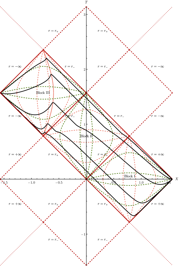
Figure 1: Penrose diagram of the symmetry axis of the Kerr spacetime for $a=M/2$. Hypersurfaces of constant time $t^{\prime}$ are plotted with solid black lines. We plot hypersurfaces corresponding to (from the bottom to the top) $t^{\prime}=-10M,-5M,0,5M,10M$. Surfaces of constant Boyer–Lindquist time $t$ are shown with green dashed lines. Orange dashed lines depict surfaces of constant tortoise radius $r_{\ast}$. A solid orange line within Block III depicts the surface with $r=0$. Details of the construction of this diagram are given in Appendix A.

II.2 Geodesic equations

Geodesic equations can be written in the Hamiltonian form as

$$\frac{dx^{\mu}}{{d\tilde{\tau}}}=\frac{\partial H}{\partial p_{\mu}},\quad\frac{dp_{\nu}}{{d\tilde{\tau}}}=-\frac{\partial H}{\partial x^{\nu}},$$ (6)

where $p^{\mu}=dx^{\mu}/d\tilde{\tau}$, $H(x^{\alpha},p_{\beta})=\frac{1}{2}g^{\mu\nu}(x^{\alpha})p_{\mu}p_{\nu}=-\frac{1}{2}m^{2}$, and $m$ is the particle rest mass. The four-velocity $u^{\mu}=dx^{\mu}/d\tau$ is normalised as $g_{\mu\nu}u^{\mu}u^{\nu}=-\delta_{1}$, where

$$\delta_{1}=\begin{cases}1&\text{for timelike geodesics},\\ 0&\text{for null geodesics}.\end{cases}$$ (7)

The above conventions imply that the affine parameter $\tilde{\tau}$ and the proper time $\tau$ are related by $\tilde{\tau}=\tau/m$.

Let the metric $g$ be given by Eq. (1) or (5). A standard reasoning shows that $H$, $E:=-p_{t}$ and $l_{z}:=p_{\varphi}$ are constants of motion. The fourth constant, referred to as the Carter constant $\mathcal{K}$, can be derived by a separation of variables in the corresponding Hamilton–Jacobi equation Carter1968 . This separation can be performed both in Boyer–Lindquist and in horizon-penetrating Kerr coordinates. Moreover, in both coordinate systems constants $H$, $E$, $l_{z}$, and $\mathcal{K}$ have the same numerical values. In particular, momentum components $p_{t}$ and $p_{\varphi}$ transform as $p_{t^{\prime}}=p_{t}=-E$ and $p_{\varphi^{\prime}}=p_{\varphi}=l_{z}$.

In Boyer–Lindquist coordinates geodesic equations can be written as

$$\rho^{2}\frac{dr}{{d\tilde{\tau}}} = \epsilon_{r}\sqrt{R(r)},$$ (8a)

$$\rho^{2}\frac{d\theta}{{d\tilde{\tau}}} = \epsilon_{\theta}\sqrt{\Theta(\theta)},$$ (8b)

$$\rho^{2}\frac{d\varphi}{{d\tilde{\tau}}} = \frac{a[(r^{2}+a^{2})E-al_{z}]}{\Delta}+\frac{1}{\sin^{2}\theta}(l_{z}-aE\sin^{2}\theta),$$ (8c)

$$\rho^{2}\frac{dt}{{d\tilde{\tau}}} = \frac{(r^{2}+a^{2})[(r^{2}+a^{2})E-al_{z}]}{\Delta}+a(l_{z}-aE\sin^{2}\theta),$$ (8d)

where we denoted

$$R(r) := [(r^{2}+a^{2})E-al_{z}]^{2}-\Delta(m^{2}r^{2}+\mathcal{K}),$$ (9a)

$$\Theta(\theta) := \mathcal{K}-m^{2}a^{2}\cos^{2}\theta-\left(\frac{l_{z}}{\sin\theta}-a\sin\theta E\right)^{2}.$$ (9b)

We will refer to $R(r)$ and $\Theta(\theta)$ as the radial and polar effective potentials, respectively. The signs $\epsilon_{r}=\pm 1$ and $\epsilon_{\theta}=\pm 1$ indicate the direction of motion with respect to the radial and polar coordinates.

There is a useful parametrization of Kerr geodesics, introduced by Mino in Mino2003 , which allows to partially decouple Eqs. (8). The so-called Mino time $\tilde{s}$ is defined by

$$\rho^{2}\frac{dx^{\mu}}{{d\tilde{\tau}}}=\frac{dx^{\mu}}{{d\tilde{s}}}$$ (10)

or

$$\tilde{\tau}=\int\limits_{0}^{\tilde{s}}\rho^{2}ds.$$ (11)

Using $\tilde{s}$ as the geodesic parameter, we obtain

$$\frac{dr}{{d\tilde{s}}} = \epsilon_{r}\sqrt{R(r)},$$ (12a)

$$\frac{d\theta}{{d\tilde{s}}} = \epsilon_{\theta}\sqrt{\Theta(\theta)},$$ (12b)

$$\frac{d\varphi}{{d\tilde{s}}} = \frac{a[(r^{2}+a^{2})E-al_{z}]}{\Delta}+\frac{1}{\sin^{2}\theta}(l_{z}-aE\sin^{2}\theta),$$ (12c)

$$\frac{dt}{{d\tilde{s}}} = \frac{(r^{2}+a^{2})[(r^{2}+a^{2})E-al_{z}]}{\Delta}+a(l_{z}-aE\sin^{2}\theta).$$ (12d)

Geodesic equations in the horizon-penetrating Kerr coordinates can be obtained simply by the following vector transformation

$$\frac{dt^{\prime}}{{d\tilde{s}}} = \frac{\partial t^{\prime}}{\partial t}\frac{dt}{d\tilde{s}}+\frac{\partial t^{\prime}}{\partial r}\frac{dr}{d\tilde{s}}=\frac{dt}{d\tilde{s}}+\frac{2Mr}{\Delta}\frac{dr}{d\tilde{s}},$$ (13a)

$$\frac{d\varphi^{\prime}}{{d\tilde{s}}} = \frac{\partial\varphi^{\prime}}{\partial\varphi}\frac{d\varphi}{d\tilde{s}}+\frac{\partial\varphi^{\prime}}{\partial r}\frac{dr}{d\tilde{s}}=\frac{d\varphi}{d\tilde{s}}+\frac{a}{\Delta}\frac{dr}{d\tilde{s}}.$$ (13b)

This gives

$$\frac{dr}{{d\tilde{s}}} = \epsilon_{r}\sqrt{R(r)},$$ (14a)

$$\frac{d\theta}{{d\tilde{s}}} = \epsilon_{\theta}\sqrt{\Theta(\theta)},$$ (14b)

$$\frac{d\varphi^{\prime}}{{d\tilde{s}}} = \frac{a[(r^{2}+a^{2})E-al_{z}]}{\Delta}+\frac{1}{\sin^{2}\theta}(l_{z}-aE\sin^{2}\theta)+\frac{a}{\Delta}\epsilon_{r}\sqrt{R(r)},$$ (14c)

$$\frac{dt^{\prime}}{{d\tilde{s}}} = \frac{(r^{2}+a^{2})[(r^{2}+a^{2})E-al_{z}]}{\Delta}+a(l_{z}-aE\sin^{2}\theta)+\frac{2Mr}{\Delta}\epsilon_{r}\sqrt{R(r)}.$$ (14d)

In the remainder of this paper we will use the following dimensionless variables:

$$a=M\alpha,\qquad t^{\prime}=MT^{\prime},\quad r=M\xi,\quad E=m\varepsilon,\quad\mathcal{K}=M^{2}m^{2}\kappa,\quad l_{z}=Mm\lambda_{z},\quad\tilde{s}=\frac{1}{Mm}s.$$ (15)

Dimensionless radii corresponding to Kerr horizons will be denoted by $\xi_{\pm}=1\pm\sqrt{1-\alpha^{2}}$. For null geodesics, for which $m=0$, the parameter $m$ in the above equations can be replaced with any mass parameter $\tilde{m}>0$.

In dimensionless variables (15), geodesic equations (14) have the form

$$\frac{d\xi}{{ds}} = \epsilon_{r}\sqrt{\tilde{R}},$$ (16a)

$$\frac{d\theta}{{ds}} = \epsilon_{\theta}\sqrt{\tilde{\Theta}},$$ (16b)

$$\frac{d\varphi^{\prime}}{{ds}} = \frac{\alpha[(\xi^{2}+\alpha^{2})\varepsilon-\alpha\lambda_{z}]}{\xi^{2}-2\xi+\alpha^{2}}+\frac{1}{\sin^{2}\theta}(\lambda_{z}-\alpha\varepsilon\sin^{2}\theta)+\frac{\alpha}{\xi^{2}-2\xi+\alpha^{2}}\epsilon_{r}\sqrt{\tilde{R}},$$ (16c)

$$\frac{dT^{\prime}}{{ds}} = \frac{(\xi^{2}+\alpha^{2})[(\xi^{2}+\alpha^{2})\varepsilon-\alpha\lambda_{z}]}{\xi^{2}-2\xi+\alpha^{2}}+\alpha(\lambda_{z}-\alpha\varepsilon\sin^{2}\theta)+\frac{2\xi}{\xi^{2}-2\xi+\alpha^{2}}\epsilon_{r}\sqrt{\tilde{R}},$$ (16d)

where

$$\tilde{R} := [(\xi^{2}+\alpha^{2})\varepsilon-\alpha\lambda_{z}]^{2}-(\xi^{2}-2\xi+\alpha^{2})(\delta_{1}\xi^{2}+\kappa),$$ (17a)

$$\tilde{\Theta} := \kappa-\delta_{1}\alpha^{2}\cos^{2}\theta-\frac{1}{\sin^{2}\theta}(\lambda_{z}-\alpha\varepsilon\sin^{2}\theta)^{2}.$$ (17b)

Note that the coordinate transformation from Boyer–Lindquist to horizon-penetrating Kerr coordinates affects only the equations for $\varphi^{\prime}$ and $T^{\prime}$, while the radial and polar equations remain unchanged. Equations (16) can also be obtained directly by working in the horizon-penetrating Kerr coordinates and by separating the variables in the Hamilton–Jacobi equation. We emphasise a connection with the Boyer–Lindquist form (12), in order to make use of solutions to Eqs. (12) derived in CHM2023 . In the next section, we review the solutions of the radial and polar equations obtained in CHM2023 and focus on equations for $\varphi^{\prime}$ and $T^{\prime}$.

III Solutions of geodesic equations

III.1 Biermann–Weierstrass formula

The form of solutions used in this work predominantly rely on the following result due to Biermann and Weierstrass biermann_1865 . Proofs of this theorem can be found in Greenhill_1892 ; Reynolds_1989 ; CM2022 .

Let $f$ be a quartic polynomial

$$f(x)=a_{0}x^{4}+4a_{1}x^{3}+6a_{2}x^{2}+4a_{3}x+a_{4},$$ (18)

and let $g_{2}$ and $g_{3}$ denote Weierstrass invariants of $f$:

$$g_{2} = a_{0}a_{4}-4a_{1}a_{3}+3a_{2}^{2},$$ (19a)

$$g_{3} = a_{0}a_{2}a_{4}+2a_{1}a_{2}a_{3}-a_{2}^{3}-a_{0}a_{3}^{2}-a_{1}^{2}a_{4}.$$ (19b)

Denote

$$z(x)=\int^{x}_{x_{0}}\frac{dx^{\prime}}{\sqrt{f(x^{\prime})}},$$ (20)

where $x_{0}$ can be any constant. Then $x$ can be expressed as

$$x=x_{0}+\frac{-\sqrt{f(x_{0})}\wp^{\prime}(z)+\frac{1}{2}f^{\prime}(x_{0})\left[\wp(z)-\frac{1}{24}f^{\prime\prime}(x_{0})\right]+\frac{1}{24}f(x_{0})f^{\prime\prime\prime}(x_{0})}{2\left[\wp(z)-\frac{1}{24}f^{\prime\prime}(x_{0})\right]^{2}-\frac{1}{48}f(x_{0})f^{(4)}(x_{0})},$$ (21)

where $\wp(z)=\wp(z;g_{2},g_{3})$ is the Weierstrass function with invariants (19). In addition

$$\wp(x) = \frac{\sqrt{f(x)f(x_{0})}+f(x_{0})}{2(x-x_{0})^{2}}+\frac{f^{\prime}(x_{0})}{4(x-x_{0})}+\frac{f^{\prime\prime}(x_{0})}{24},$$ (22a)

$$\wp^{\prime}(x) = -\left[\frac{f(x)}{(x-x_{0})^{3}}-\frac{f^{\prime}(x_{0})}{4(x-x_{0})}\right]\sqrt{f(x_{0})}-\left[\frac{f(x)}{(x-x_{0})^{3}}+\frac{f^{\prime}(x_{0})}{4(x-x_{0})}\right]\sqrt{f(x)}.$$ (22b)

III.2 Radial motion

The dimensionless radial potential $\tilde{R}$ can be written as

$$\tilde{R}(\xi)=a_{0}\xi^{4}+4a_{1}\xi^{3}+6a_{2}\xi^{2}+4a_{3}\xi+a_{4},$$ (23)

where

$$a_{0} = \varepsilon^{2}-\delta_{1},$$ (24a)

$$a_{1} = \frac{1}{2}\delta_{1},$$ (24b)

$$a_{2} = -\frac{1}{6}(\delta_{1}\alpha^{2}+\kappa-2\alpha^{2}\varepsilon^{2}+2\alpha\varepsilon\lambda_{z}),$$ (24c)

$$a_{3} = \frac{1}{2}\kappa,$$ (24d)

$$a_{4} = \alpha^{4}\varepsilon^{2}-\alpha^{2}\kappa-2\alpha^{3}\varepsilon\lambda_{z}+\alpha^{2}\lambda_{z}^{2}=-\alpha^{2}[\kappa-(\alpha\varepsilon-\lambda_{z})^{2}].$$ (24e)

Weierstrass invariants associated with the coefficients (24) will be denoted by

$$g_{\tilde{R},2} = a_{0}a_{4}-4a_{1}a_{3}+3a_{2}^{2},$$ (25a)

$$g_{\tilde{R},3} = a_{0}a_{2}a_{4}+2a_{1}a_{2}a_{3}-a_{2}^{3}-a_{0}a_{3}^{2}-a_{1}^{2}a_{4}.$$ (25b)

A direct application of the Biermann–Weierstrass theorem to Eq. (16a) yields the formula for $\xi=\xi(s)$,

$$\xi(s)=\xi_{0}+\frac{-\epsilon_{r,0}\sqrt{\tilde{R}(\xi_{0})}\wp^{\prime}_{\tilde{R}}(s)+\frac{1}{2}\tilde{R}^{\prime}\xi_{0})[\wp_{\tilde{R}}(s)-\frac{1}{24}\tilde{R}^{\prime\prime}(\xi_{0})]+\frac{1}{24}\tilde{R}(\xi_{0})\tilde{R}^{\prime\prime\prime}(\xi_{0})]}{2[\wp_{\tilde{R}}(s)-\frac{1}{24}\tilde{R}^{\prime\prime}(\xi_{0})]^{2}-\frac{1}{48}\tilde{R}(\xi_{0})\tilde{R}^{(4)}(\xi_{0})},$$ (26)

where $\wp_{\tilde{R}}(s)=\wp_{\tilde{R}}(s;g_{\tilde{R},2}g_{\tilde{R},3})$ is the Weierstrass function with invariants (25), and $\xi_{0}=\xi(0)$ is an arbitrarily selected initial radius corresponding to $s=0$. In Equation (26) the sign $\epsilon_{r,0}=\pm 1$ denotes a value of $\epsilon_{r}$ corresponding to the initial location $\xi_{0}$. In other words, $\epsilon_{r,0}$ is a part of initial data (initial parameter), while the sign $\epsilon_{r}$ can change along a given geodesic.

III.3 Polar motion

Equation (16b) can be transformed to the Biermann–Weierstrass form by a substitution $\mu=\cos\theta$, which provides a one to one mapping for $0\leq\theta\leq\pi$. Defining $g(\mu):=\sin^{2}\theta\tilde{\Theta}(\theta)$, we get

$$\frac{d\mu(s)}{ds}=-\epsilon_{\theta}\sqrt{g(\mu)}.$$ (27)

The function $g(\mu)$ is a polynomial with respect to $\mu$ given by

$$g(\mu)=b_{0}\mu^{4}+6b_{2}\mu^{2}+b_{4},$$ (28)

where the coefficients $b_{0}$, $b_{2}$, and $b_{4}$ can be expressed as

$$b_{0} = -\alpha^{2}\left(\varepsilon^{2}-\delta_{1}\right)=-\alpha^{2}a_{0},$$ (29a)

$$b_{2} = \frac{1}{6}\left(-\alpha^{2}\delta_{1}+2\alpha^{2}\varepsilon^{2}-\kappa-2\alpha\varepsilon\lambda_{z}\right)=a_{2},$$ (29b)

$$b_{4} = -\alpha^{2}\varepsilon^{2}+\kappa+2\alpha\varepsilon\lambda_{z}-\lambda_{z}^{2}=\kappa-(\alpha\varepsilon-\lambda_{z})^{2}=-\frac{a_{4}}{\alpha^{2}},$$ (29c)

and $a_{0}$, $a_{2}$, and $a_{4}$ are given by Eqs. (24). Weierstrass invariants associated with coefficients $b_{0}$, $b_{2}$, and $b_{4}$ can be written as

$$g_{g,2} = b_{0}b_{4}+3b_{2}^{2},$$ (30a)

$$g_{g,3} = b_{0}b_{2}b_{4}-b_{2}^{3}.$$ (30b)

Again, using the Biermann–Weierstrass formula, one can write the expression for $\mu=\mu(s)$ in the form

$$\mu(s)=\mu_{0}+\frac{\epsilon_{\theta,0}\sqrt{g(\mu_{0})}\wp^{\prime}_{g}(s)+\frac{1}{2}g^{\prime}(\mu_{0})[\wp_{g}(s)-\frac{1}{24}g^{\prime\prime}(\mu_{0})]+\frac{1}{24}g(\mu_{0})g^{\prime\prime\prime}(\mu_{0})]}{2[\wp_{g}(s)-\frac{1}{24}g^{\prime\prime}(\mu_{0})]^{2}-\frac{1}{48}g(\mu_{0})g^{(4)}(\mu_{0})},$$ (31)

where $\wp_{g}(s)=\wp_{g}(s;g_{g,2}g_{g,3})$ and $\mu_{0}=\mu(0)=\cos\theta_{0}=\cos\theta(0)$ represents an initial value corresponding to $s=0$. As in Eq. (26), the sign $\epsilon_{\theta,0}=\pm 1$ is a parameter equal to $\epsilon_{\theta}$ at $\theta=\theta_{0}$, and it remains constant along the entire geodesic. A more detailed discussion of solutions (26) and (31) can be found in CHM2023 .

III.4 Azimuthal motion

Equation (16c) consists of a component related to the azimuthal motion in Boyer–Lindquist coordinates and an additional term, dependent on $\xi(s)$, arising from transformation (4). We will first treat the two components separately and then discuss their sum, which may remain regular across the horizons. An integration with respect to the Mino time $s$ yields

$$\varphi^{\prime}(s)-\varphi^{\prime}(0) = \int_{0}^{s}\left\{\frac{\alpha[(\xi^{2}(\bar{s})+\alpha^{2})\varepsilon-\alpha\lambda_{z}]}{\xi^{2}(\bar{s})-2\xi(\bar{s})+\alpha^{2}}+\frac{1}{\sin^{2}\theta(\bar{s})}\left[\lambda_{z}-\alpha\varepsilon\sin^{2}\theta(\bar{s})\right]\right\}d\bar{s}+\int_{0}^{s}\frac{\alpha\epsilon_{r}\sqrt{\tilde{R}(\bar{s})}}{\xi^{2}(\bar{s})-2\xi(\bar{s})+\alpha^{2}}d\bar{s}$$

$$= \alpha\int_{0}^{s}\frac{2\xi(\bar{s})\varepsilon-\alpha\lambda_{z}}{\xi^{2}(\bar{s})-2\xi(\bar{s})+\alpha^{2}}d\bar{s}+\lambda_{z}\int_{0}^{s}\frac{d\bar{s}}{\sin^{2}\theta(\bar{s})}+\alpha\int_{0}^{s}\frac{\epsilon_{r}\sqrt{\tilde{R}(\bar{s})}}{\xi^{2}(\bar{s})-2\xi(\bar{s})+\alpha^{2}}d\bar{s}$$

$$= J_{\mathrm{BL}}(s)+J_{\xi}(s),$$ (33)

where $J_{\mathrm{BL}}(s):=\tilde{J}_{\mathrm{BL}}(s)+J_{\theta}(s)$ and

$$\tilde{J}_{\mathrm{BL}}(s) := \alpha\int_{0}^{s}\frac{2\xi(\bar{s})\varepsilon-\alpha\lambda_{z}}{\xi^{2}(\bar{s})-2\xi(\bar{s})+\alpha^{2}}d\bar{s},$$ (34)

$$J_{\theta}(s) := \lambda_{z}\int_{0}^{s}\frac{d\bar{s}}{\sin^{2}\theta(\bar{s})},$$ (35)

$$J_{\xi}(s) := \alpha\int_{0}^{s}\frac{\epsilon_{r}\sqrt{\tilde{R}(\bar{s})}}{\xi^{2}(\bar{s})-2\xi(\bar{s})+\alpha^{2}}d\bar{s}.$$ (36)

Integrals $\tilde{J}_{\mathrm{BL}}$ and $J_{\theta}$ were expressed in terms of Weierstrass functions in CHM2023 . To obtain a solution for Eq. (36), we write

$$J_{\xi}(s)=\alpha\int_{0}^{s}\frac{d\xi(\bar{s})/d\bar{s}}{\xi^{2}(\bar{s})-2\xi(\bar{s})+\alpha^{2}}d\bar{s}.$$ (37)

For a segment of a geodesic along which $\xi=\xi(s)$ is monotonic, one change the integration variable to $\xi$ and write

$$J_{\xi}(s)=\alpha\int_{\xi_{0}}^{\xi(s)}\frac{d\bar{\xi}}{\bar{\xi}^{2}-2\bar{\xi}+\alpha^{2}}=\alpha\left[\frac{\arctan\left(\frac{\xi(s)-1}{\sqrt{\alpha^{2}-1}}\right)}{\sqrt{\alpha^{2}-1}}-\frac{\arctan\left(\frac{\xi_{0}-1}{\sqrt{\alpha^{2}-1}}\right)}{\sqrt{\alpha^{2}-1}}\right],$$ (38)

which, together with Eq. (26), provides the solution. Note that due to the symmetry of Eq. (16a), expression (38) remains valid also for trajectories passing through radial turning points.

The integrals $J_{\mathrm{BL}}$ and $J_{\xi}$ are, generically, divergent at the horizons, i.e., for $s$ such that $\xi(s)=\xi_{\pm}$, but the sum $J_{\mathrm{BL}}+J_{\xi}$ can remain regular. A direct calculation shows that $J_{\text{BL}}(s)$ and $J_{\xi}(s)$ can be expressed in the form

$$\tilde{J}_{\mathrm{BL}}(s)+J_{\xi}(s)=\alpha\int_{0}^{s}\left\{\frac{\delta_{1}\xi^{2}(\bar{s})+\kappa}{[\xi^{2}(\bar{s})+\alpha^{2}]\varepsilon-\alpha\lambda_{z}-d\xi(\bar{s})/d\bar{s}}-\varepsilon\right\}d\bar{s}.$$ (39)

The integrand in Eq. (39) can be divergent, if

$$[\xi^{2}(s)+\alpha^{2}]\varepsilon-\alpha\lambda_{z}-\frac{d\xi(s)}{ds}=0$$ (40)

or, equivalently,

$$[\xi^{2}(s)+\alpha^{2}]\varepsilon-\alpha\lambda_{z}=\epsilon_{r}\sqrt{\tilde{R}}.$$ (41)

By computing the square of the above equation we see that this can only happen, if

$$[\xi^{2}(s)-2\xi(s)+\alpha^{2}][\delta_{1}\xi^{2}(s)+\kappa]=0,$$

that is at $\xi(s)=\xi_{\pm}$. On the other hand, the expression $[\xi^{2}(s)+\alpha^{2}]\varepsilon-\alpha\lambda_{z}-d\xi(s)/ds$ can be clearly non-zero at the horizon, depending on the sign $\epsilon_{r}$. In our examples discussed in Sec. IV this happens for $\epsilon_{r}=-1$, i.e., for incoming geodesics. In general, if the sign of $[\xi^{2}(s)+\alpha^{2}]\varepsilon-\alpha\lambda_{z}$ can be controlled, one can exclude the possibility that $\tilde{J}_{\mathrm{BL}}$ diverges at the horizon. For instance, for $[\xi^{2}(s)+\alpha^{2}]\varepsilon-\alpha\lambda_{z}>0$ and $\epsilon_{r}=-1$, the denominator in Eq. (39) remains strictly positive. We discuss this problem in more detail in Sec. III.6.

III.5 Time coordinate

Similarly to the equation for $\varphi^{\prime}$, the right-hand side of Eq. (16d) also consist of a Boyer–Lindquist term and a term associated with the transformation to horizon-penetrating Kerr coordinates. Integrating Eq. (16d) one gets

$$T^{\prime}(s)-T^{\prime}(0) = \int_{0}^{s}\left\{\frac{[\xi^{2}(\bar{s})+\alpha^{2}][(\xi^{2}(\bar{s})+\alpha^{2})\varepsilon-\alpha\lambda_{z}]}{\xi^{2}(\bar{s})-2\xi(\bar{s})+\alpha^{2}}+\alpha[\lambda_{z}-\alpha\varepsilon\sin^{2}\theta(\bar{s})]\right\}d\bar{s}$$ (42)

$$+\int_{0}^{s}\frac{2\xi(\bar{s})\epsilon_{r}\sqrt{\tilde{R}(\bar{s})}}{\xi^{2}(\bar{s})-2\xi(\bar{s})+\alpha^{2}}d\bar{s}$$

$$= N_{\text{BL}}(s)+N_{\xi}(s).$$

Here

$$N_{\text{BL}}(s) := \int_{0}^{s}\left\{\frac{[\xi^{2}(\bar{s})+\alpha^{2}][(\xi^{2}(\bar{s})+\alpha^{2})\varepsilon-\alpha\lambda_{z}]}{\xi^{2}(\bar{s})-2\xi(\bar{s})+\alpha^{2}}+\alpha(\lambda_{z}-\alpha\varepsilon\sin^{2}\theta(\bar{s}))\right\}d\bar{s}$$ (43)

$$= \tilde{N}_{\mathrm{BL}}(s)-\alpha^{2}\varepsilon N_{\theta}(s),$$

where

$$\tilde{N}_{\mathrm{BL}}(s) := \int_{0}^{s}\frac{\left[\xi^{2}(\bar{s})+\alpha^{2}\right]^{2}\varepsilon-2\alpha\lambda_{z}\xi(\bar{s})}{\xi^{2}(\bar{s})-2\xi(\bar{s})+\alpha^{2}}d\bar{s},$$ (44)

$$N_{\theta}(s) := \int_{0}^{s}\sin^{2}\theta(\bar{s})d\bar{s},$$ (45)

and

$$N_{\xi}(s):=2\int_{0}^{s}\frac{\xi(\bar{s})\epsilon_{r}\sqrt{\tilde{R}(\bar{s})}}{\xi^{2}(\bar{s})-2\xi(\bar{s})+\alpha^{2}}d\bar{s}.$$ (46)

The integrals $\tilde{N}_{\mathrm{BL}}(s)$ and $N_{\theta}(s)$ were computed in CHM2023 .

As before, we start by evaluating the integral in Eq. (46), which we write in the form

$$N_{\xi}(s)=2\int_{0}^{s}\frac{\xi(\bar{s})}{\xi^{2}(\bar{s})-2\xi(\bar{s})+\alpha^{2}}\frac{d\xi(\bar{s})}{d\bar{s}}d\bar{s}.$$ (47)

Changing the integration variable form $s$ to $\xi=\xi(s)$ we obtain

$$N_{\xi}(s)=2\int_{\xi_{0}}^{\xi(s)}\frac{\bar{\xi}}{\bar{\xi}^{2}-2\bar{\xi}+\alpha^{2}}d\bar{\xi}=\log\left[\frac{\xi^{2}(s)-2\xi(s)+\alpha^{2}}{\xi_{0}^{2}-2\xi_{0}+\alpha^{2}}\right]+2\left[\frac{\arctan\left(\frac{\xi(s)-1}{\sqrt{\alpha^{2}-1}}\right)}{\sqrt{\alpha^{2}-1}}-\frac{\arctan\left(\frac{\xi_{0}-1}{\sqrt{\alpha^{2}-1}}\right)}{\sqrt{\alpha^{2}-1}}\right],$$ (48)

which again together with Eq. (26) provides the solution.

A regularization of the sum $\tilde{N}_{\mathrm{BL}}(s)+N_{\xi}(s)$ can be done in many ways. One of them is, however, particularly convenient. Note that

$$\frac{(\xi^{2}+\alpha^{2})^{2}\varepsilon-2\alpha\lambda_{z}\xi}{\xi^{2}-2\xi+\alpha^{2}}=(\xi^{2}+\alpha^{2})\varepsilon+\frac{2\xi\left[(\xi^{2}+\alpha^{2})\varepsilon-\alpha\lambda_{z}\right]}{\xi^{2}-2\xi+\alpha^{2}}.$$ (49)

Therefore,

$$\tilde{N}_{\mathrm{BL}}(s)+N_{\xi}(s) = \int_{0}^{s}\left\{\frac{2\xi(\bar{s})\left[(\xi^{2}(\bar{s})+\alpha^{2})\varepsilon-\alpha\lambda_{z}+d\xi(\bar{s})/d\bar{s}\right]}{\xi^{2}(\bar{s})-2\xi(\bar{s})+\alpha^{2}}+[\xi^{2}(\bar{s})+\alpha^{2}]\varepsilon\right\}d\bar{s}$$ (50)

$$= \int_{0}^{s}\left\{\frac{2\xi(\bar{s})\left[\delta_{1}\xi^{2}(\bar{s})+\kappa\right]}{[\xi^{2}(\bar{s})+\alpha^{2}]\varepsilon-\alpha\lambda_{z}-d\xi(\bar{s})/d\bar{s}}+[\xi^{2}(\bar{s})+\alpha^{2}]\varepsilon\right\}d\bar{s}.$$

The advantage of this choice is that now a potentially problematic denominator in Eq. (50) has the same form as in Eq. (39).

III.6 Regularity at horizons

We see from preceding subsections that the regularity of the expressions for $\varphi^{\prime}$ and $T^{\prime}$ depends on the signs of

$$A:=(\xi^{2}+\alpha^{2})\varepsilon-\alpha\lambda_{z}$$ (51)

and $\epsilon_{r}$. It can be shown that for timelike future-directed geodesics at $\xi>\xi_{+}$ (in Boyer–Lindquist Block I), one has $A>0$. Thus, by continuity, for $\epsilon_{r}=-1$ (incoming geodesics) and $\tilde{R}>0$, we have $A-d\xi(s)/ds=A-\epsilon_{r}\sqrt{\tilde{R}}>0$ up to the horizon at $\xi_{+}$. Hence, for incoming future-directed timelike geodesics both $\varphi^{\prime}$ and $T^{\prime}$ remain regular at the event horizon joining Blocks I and II.

A proof that for a timelike future-directed geodesic at $\xi>\xi_{+}$, one must have $A>0$ can be found in Rioseco2024 , but we repeat it here for completeness. Note first that the vector

$$N=\left(1+\frac{2Mr}{\rho^{2}}\right)\partial_{t^{\prime}}-\frac{2Mr}{\rho^{2}}\partial_{r}$$ (52)

is normal to hypersurfaces of constant time $t^{\prime}$. Lowering the indices in $N$ one gets $N_{\mu}=(-1,0,0,0)$. Since $g(N,N)=-(1+2Mr/\rho^{2})$, it is also timelike, as long as $r>0$. This vector defines a time orientation. Consider a vector

$$X:=(r^{2}+a^{2})\partial_{t^{\prime}}+a\partial_{\varphi^{\prime}}.$$ (53)

O’Neill refers to $X$ as one of “the canonical Kerr vector fields” (Neill1995 , p. 60). It satisfies $g(X,X)=-\rho^{2}\Delta$, and thus it is timelike for $\Delta>0$, i.e., for $r<r_{-}$ or $r>r_{+}$ (in Blocks I and III). It is also future-directed, since $g(N,X)=-dt^{\prime}(X)=-(r^{2}+a^{2})<0$. On the other hand,

$$p(X)=(r^{2}+a^{2})p_{t^{\prime}}+ap_{\varphi^{\prime}}=-\left[(r^{2}+a^{2})E-al_{z}\right]=-M^{2}m\left[(\xi^{2}+\alpha^{2})\varepsilon-\alpha\lambda_{z}\right],$$ (54)

where $p$ denotes the momentum covector. A future-directed momentum $p$ has to satisfy $p(X)<0$, and hence $A=(\xi^{2}+\alpha^{2})\varepsilon-\alpha\lambda_{z}>0$. We emphasise that negative values of $\varepsilon$ are still allowed within the ergosphere.

In Block II, where $\Delta<0$, i.e., for $r_{-}<r<r_{+}$, Rioseco and Sarbach Rioseco2024 propose to use the vector

$$Y:=2Mr\partial_{t^{\prime}}+\Delta\partial_{r}+a\partial_{\varphi^{\prime}}.$$ (55)

It satisfies $g(Y,Y)=\rho^{2}\Delta$ and, consequently, it is timelike for $r_{-}<r<r_{+}$. Since $g(N,Y)=-dt^{\prime}(Y)=-2Mr$, it is also future-directed in $r_{-}<r<r_{+}$. On the other hand,

$$p(Y)=2Mrp_{t^{\prime}}+\Delta p_{r}+ap_{\varphi^{\prime}}=-2MrE+\Delta p_{r}+al_{z}.$$ (56)

Since $\Delta p_{r}=\epsilon_{r}\sqrt{R}+2MrE-al_{z}$, we get $p(Y)=\epsilon_{r}\sqrt{R}$. Thus in Block II, the momentum $p$ can be future-directed only for $\epsilon_{r}=-1$.

Turning to the “regularization” applied in Eqs. (39) and (50) note that it is based on the observation that

$$A^{2}-\tilde{R}=(\xi^{2}-2\xi+\alpha^{2})(\delta_{1}\xi^{2}+\kappa),$$ (57)

and hence $A^{2}-\tilde{R}$ has two real zeros, precisely at $\xi=\xi_{\pm}$. On the other hand

$$A^{2}-\tilde{R}=\left(A-\epsilon_{r}\sqrt{\tilde{R}}\right)\left(A+\epsilon_{r}\sqrt{\tilde{R}}\right)=\left(A-\frac{d\xi}{ds}\right)\left(A+\frac{d\xi}{ds}\right).$$ (58)

Thus, if $A-\epsilon_{r}\sqrt{\tilde{R}}$ remains non-zero at a given radius $\xi=\xi_{+}$ or $\xi=\xi_{-}$, then $A+\epsilon_{r}\sqrt{\tilde{R}}$ must be zero for the same radius, and vice versa. In other words, horizon-penetrating Kerr coordinates do not allow for a description in which a given trajectory can cross smoothly horizons at $\xi=\xi_{+}$ or $\xi=\xi_{-}$ in both radial directions $\epsilon_{r}=\pm 1$ at the same time. This is, of course, consistent with the behavior shown in Fig. 1. Suppose that a given trajectory passes from Block I to Block II, and then to Block III, where it encounters a radial turning point and continues further with $\epsilon_{r}=+1$. Such a trajectory will hit the Cauchy horizon at $\xi=\xi_{-}$ with $\epsilon_{r}=+1$, where both $T^{\prime}$ and $\varphi^{\prime}$ would diverge. We show this behavior in particular examples in Sec. IV. It would also be tempting to illustrate this situation directly in the Penrose diagram in Fig. 1, which is however plotted for points at the axis, and assuming that $d\theta=d\varphi=0$. An illustration of this kind should be possible in terms of projection diagrams defined in Chrusciel2012 . Unfortunately, from the computational point of view, such diagrams are much more difficult to draw exactly.

IV Examples

Table 1: Parameters of geodesics shown in Figs. 2 to 9. In all examples $\alpha=0.8$, $\theta_{0}=0.85$, $\varphi_{0}^{\prime}=0.33$.

Fig. No.	$\delta_{1}$	$\varepsilon^{2}$	$\kappa$	$\lambda_{z}$	$\alpha$	Real zeros of $\tilde{R}(\xi)$	Real zeros of $\tilde{\Theta}(\theta)$	$\xi_{0}$
2	1	1.1	12	$-1$	0.8	$-24.3351$,  0.254136	2.81429,  0.327303	8
3	1	0.95	12	3	0.8	$\begin{array}[]{c}0.22019,\,1.63896,\\ 8.44487,\,29.696\end{array}$	2.29552,  0.846071	10
4	1	1.1	12	3	0.8	$\begin{array}[]{c}-26.4861,\,0.230431,\\ 1.67987,\,4.57578\end{array}$	2.30596,  0.835636	10
5	1	30	12	$-0.05$	0.8	—	$\begin{array}[]{c}3.12646,\,2.2675,\\ 0.874094,\,0.0151329\end{array}$	10
6	0	1	60	4.47214	0.8	$\begin{array}[]{c}-8.927,\,0.296172,\\ 1.60191,\,7.02892\end{array}$	2.56341,  0.578185	10
7	0	1	0.6	$-0.111803$	0.8	$-0.721257$,  $-0.137167$	$\begin{array}[]{c}2.96415,\,2.22796,\\ 0.913634,\,0.177447\end{array}$	10
8	0	1	0.4	$-0.00912871$	0.8	—	$\begin{array}[]{c}3.12688,\,2.25351,\\ 0.88808,\,0.0147079\end{array}$	10
9	1	1.1	10	$-0.2$	0.8	$-3.59963$,  0.329668	3.0772,  0.0643885	12

In this section we discuss a collection of sample solutions obtained with the help of formulas derived in preceding sections.

We perform our computations using Wolfram Mathematica wolfram . The formulas for $\xi(s)$ and $\mu(s)$, or equivalently $\theta(s)$, can be encoded directly. The formulas for the azimuthal angle $\varphi^{\prime}(s)$ and the time $T^{\prime}(s)$ require a regularization, if a geodesic crosses one of the horizons. In practice, we substitute in Eq. (39) expressions for $\xi(s)$ and $\theta(s)$ given by Eqs. (26) and (31), and evaluate the resulting integral numerically. In principle, the derivative $d\xi(s)/ds$ in Eq. (39) could be expressed as $d\xi(s)/ds=\epsilon_{r}\sqrt{\tilde{R}}$, by virtue of Eq. (16a). Using this form turns out to be problematic, as it requires knowledge of the sign $\epsilon_{r}$, which changes at the radial turning points. To circumvent this difficulty, we use in Eq. (39) the derivative $d\xi(s)/ds$ obtained by a direct differentiation of Eq. (26). Although the integral (39) can be evaluated analytically, similarly to the calculation presented in CHM2023 , we find computing it numerically to be quite effective. In a sense, we try to combine in our implementation the best of the two approaches—elegant formulas for the radial and polar coordinates and relatively straightforward numerical integrals providing $\varphi^{\prime}$ and the time coordinate $T^{\prime}$.

Figures 2 to 9 depict our solutions obtained for various parameters, collected in Table 1. They show the orbits in $\xi$–$\theta$ and $\xi$–$\varphi^{\prime}$ planes and in the three-dimensional space. We use Cartesian coordinates $(x,y,z)$ defined as

$$x = \xi\cos\varphi^{\prime}\sin\theta,$$ (59a)

$$y = \xi\sin\varphi^{\prime}\sin\theta,$$ (59b)

$$z = \xi\cos\theta.$$ (59c)

In Table 1 we provide also real zeros of $\tilde{R}(\xi)$, corresponding to radial turning points, as well as zeros of $\tilde{\Theta}(\theta)$. The latter define the angular ranges available for the motion along a given geodesic. We illustrate these ranges by drawing appropriate cones in three-dimensional plots or lines in $\xi$–$\theta$ plane plots. Kerr horizons at $\xi=\xi_{\pm}$ are depicted as spheres or circles. Finally, as a double-check of our results, we plot solutions obtained by solving numerically the Kerr geodesic equations. These numerical solutions are depicted with dotted lines. For simplicity, we omit the prime in $\varphi^{\prime}$ in labels of all figures in this paper.

Figure 2 shows an unbound timelike trajectory, plunging into the black hole. The trajectory crosses smoothly both horizons at $\xi=\xi_{\pm}$ and encounters a radial turning point located at $0<\xi<\xi_{-}$. The solution for $\varphi^{\prime}$ can be continued smoothly up to the Cauchy horizon at $\xi=\xi_{-}$, where it diverges.

Figure 3 shows a standard timelike bound geodesic, corresponding to a “Keplerian” motion. In Fig. 4, we depict an unbound timelike orbit, which does not plunge into the black hole.

A very interesting case is shown in Fig. 5, depicting a timelike unbound trajectory crossing smoothly both horizons at $\xi=\xi_{\pm}$. This trajectory does not encounter a radial turning point and consequently it continues, in the extended Kerr spacetime, to negative radii $\xi$ (Boyer–Lindquist Block III, see also Hawking1973 , p. 163). In the terminology of Neill1995 such orbits are referred to as “transits”. We illustrate the transition from $\xi>0$ to $\xi<0$ by plotting a segment of the geodesic corresponding to $\xi>0$ in orange, and a segment corresponding to $\xi<0$ in purple. Note that Cartesian coordinates defined by Eq. (59) allow for a change from positive to negative values of the radius, which corresponds simply to the reflection $x\to-x$, $y\to-y$, $z\to-z$, or equivalently, to a change of angular coordinates. To avoid confusion, apart from using two colors in the graphs, we also provide a plot of the radius $\xi$ versus the Mino time $s$. Since no horizons occur for $\xi<0$, the trajectory can be continued smoothly to $\xi\to-\infty$. Note that the apparent reflection of Cartesian coordinates associated with the transition from $\xi>0$ to $\xi<0$ creates (in the plots) a false impression of a reflection in the polar angle $\theta$, as well as an impression that the trajectory leaves the bounds of the allowed polar motion, given by zeros of $\tilde{\Theta}(\theta)$. In reality, $\theta$ remains safely within the allowed range along the entire geodesic trajectory.

Figure 6 shows an example of an unbound null geodesic, scattered by the black hole. In Fig. 7, we also deal with a null geodesic, but it is much more interesting. This trajectory crosses smoothly both horizons and continues to negative values of $\xi$, where it encounters a radial turning point. It then re-enters the region with $\xi>0$ and can be continued up to the Cauchy horizon at $\xi=\xi_{-}$. In Fig. 7 a segment corresponding to negative radii is again marked in purple, while a segment with positive radii is plotted in orange.

Figure 8 illustrates a behavior similar to the one depicted in Fig. 5, but obtained for a null geodesic. The trajectory plunges into the black hole and continues to negative radii. Figure 9 shows another timelike geodesic with a behavior similar to the one illustrated in Fig. 2.

Finally, in Fig. 10 we plot a collection of more or less random timelike geodesics plunging into the black hole. In this case we only show segments of geodesics located outside the black hole horizon (although they can be continued into the black hole). With this plot we aim to show that, when visualized in horizon-penetrating Kerr coordinates, the geodesics plunging into the black hole do not make an impression of swirling around the horizon—a behavior present in the Boyer–Lindquist coordinates. Our Fig. 10 should be contrasted, e.g., with Fig. 6 in Dyson2023 .

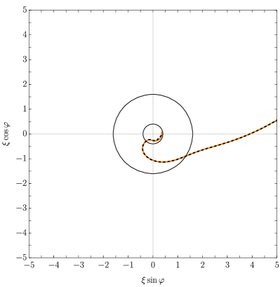
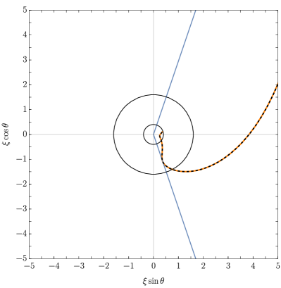
Figure 2: A timelike orbit with $\varepsilon^{2}=1.1$, $\lambda_{z}=-1$, $\alpha=0.8$, $\kappa=12$ and initial position at $\xi_{0}=8$, $\theta_{0}=0.85$, $\epsilon_{r,0}=-1$, $\epsilon_{\theta,0}=1$.

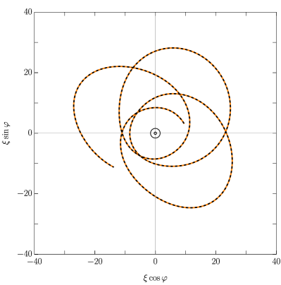
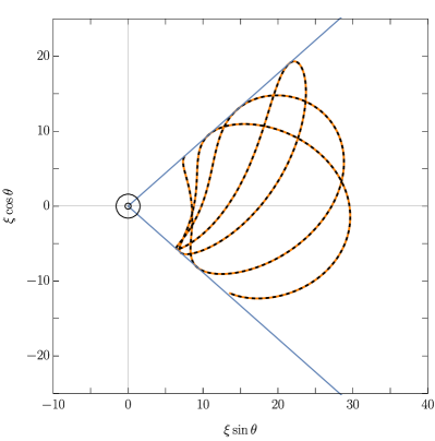
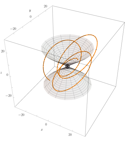
Figure 3: Same as in Fig. 2, but for a timelike bound orbit with $\varepsilon^{2}=0.95$, $\lambda_{z}=3$, $\alpha=0.8$, $\kappa=12$, and an initial position at $\xi_{0}=10$, $\theta_{0}=0.85$, $\epsilon_{r,0}=-1$, $\epsilon_{\theta,0}=1$.

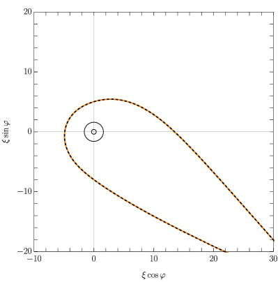
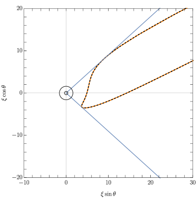
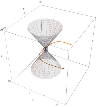
Figure 4: Same as in Fig. 2, but for a timelike unbound scattered orbit with $\varepsilon^{2}=1.1$, $\lambda_{z}=3$, $\alpha=0.8$, $\kappa=12$, and an initial position at $\xi_{0}=10$, $\theta_{0}=0.85$, $\epsilon_{r,0}=-1$, $\epsilon_{\theta,0}=1$.

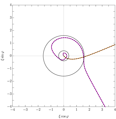
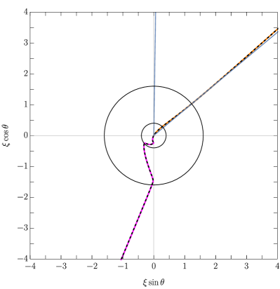
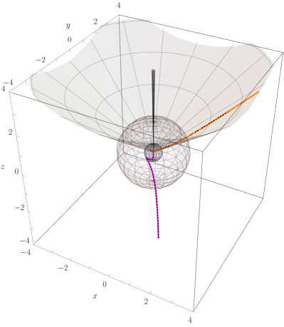
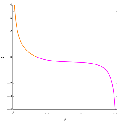
Figure 5: A timelike orbit with $\varepsilon^{2}=30$, $\lambda_{z}=-0.05$, $\alpha=0.8$, $\kappa=12$, and initial position at $\xi_{0}=10$, $\theta_{0}=0.85$, $\epsilon_{r,0}=-1$, $\epsilon_{\theta,0}=1$. A part of the trajectory with $\xi<0$ is marked in purple.

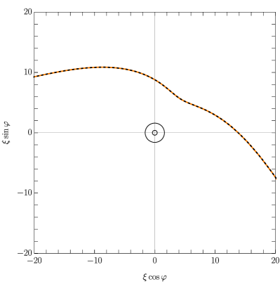
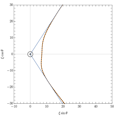
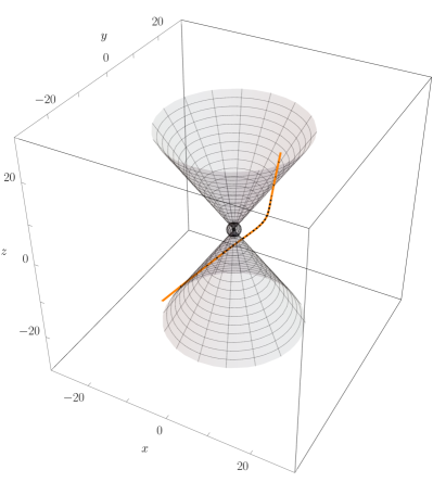
Figure 6: Same as in Fig. 2, but for a null unbound orbit with $\varepsilon^{2}=1$, $\lambda_{z}\approx 4.47214$, $\alpha=0.8$, $\kappa=60$, and an initial position at $\xi_{0}=10$, $\theta_{0}=0.85$, $\epsilon_{r,0}=-1$, $\epsilon_{\theta,0}=1$.

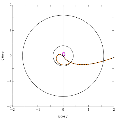
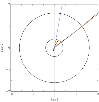
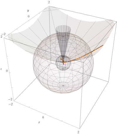
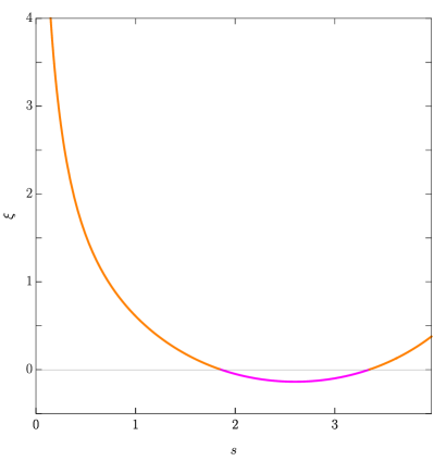
Figure 7: A null orbit with $\varepsilon^{2}=1$, $\lambda_{z}=-0.111803$, $\alpha=0.8$, $\kappa=0.6$ and initial position at $\xi_{0}=10$, $\theta_{0}=0.85$, $\epsilon_{r,0}=-1$, $\epsilon_{\theta,0}=1$.

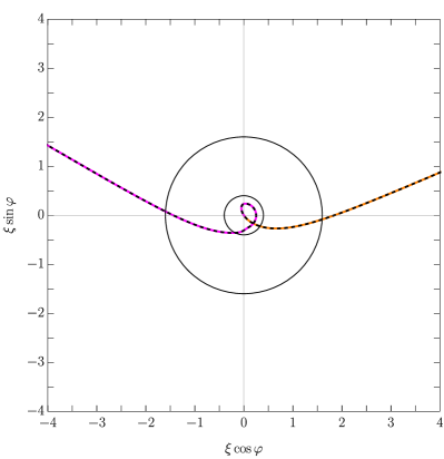
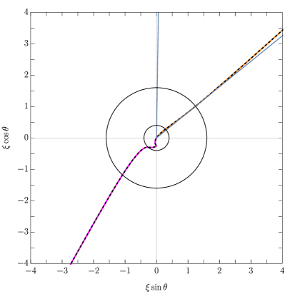
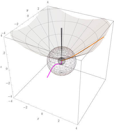
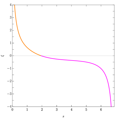
Figure 8: A null orbit with $\varepsilon^{2}=1$, $\lambda_{z}=-0.00912871$, $\alpha=0.8$, $\kappa=0.4$, and initial position at $\xi_{0}=10$, $\theta_{0}=0.85$, $\epsilon_{r,0}=-1$, $\epsilon_{\theta,0}=1$.

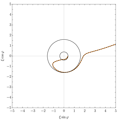
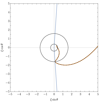
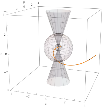
Figure 9: A timelike orbit with $\varepsilon^{2}=1.1$, $\lambda_{z}=-0.2$, $\alpha=0.8$, $\kappa=10$ and initial position at $\xi_{0}=12$, $\theta_{0}=0.85$, $\epsilon_{r,0}=-1$, $\epsilon_{\theta,0}=1$.

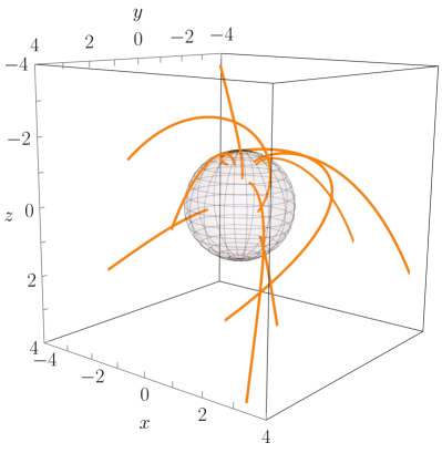
Figure 10: A sample of timelike geodesics plunging into the black hole. The event horizon is depicted as a gray sphere. Geodesics are only plotted up to the horizon. This plot can be compared with similar ones made in Boyer–Lindquist coordinates (see, e.g., Fig. 6 in Dyson2023 )

.

V Summary

We provided a description of timelike and null Kerr geodesics in horizon-penetrating Kerr coordinates, extending a recent analysis of CHM2023 . From the technical point of view, the change from Boyer–Lindquist coordinates used in CHM2023 to the horizon-penetrating Kerr coordinate system only slightly affects our formalism. The radial and polar equations remain unchanged, which allows us to use relatively compact formulas (26) and (31) for the radial and polar coordinates. Additional terms appear in equations for the azimuthal and time coordinates, but they can be integrated, once the solution to the radial equation is known. Our formulas (38) and (48) provide, together with Eq. (26), all necessary expressions.

The horizon-penetrating Kerr coordinate system allows for a continuation of geodesics across horizons within the region of the extended Kerr spacetime in which it is well-defined, i.e., within Boyer–Lindquist Blocks I, II, and III (Fig. 1). At the level of geodesic equations, regularity at the horizons depends explicitly on the radial direction of motion. A reasoning given in Sec. III.6 and our examples of Sec. IV provide the following generic picture. A future-directed timelike or null geodesic originating outside the black hole (in Block I) and moving inward ($\epsilon_{r}=-1$) can encounter a radial turning point at $r>r_{+}$ or it can pass smoothly through the event ($r=r_{+}$) and the Cauchy ($r=r_{-}$) horizons, transiting through Block II to Block III. In Block III a trajectory may continue smoothly to $r\to-\infty$ (the so-called transit orbit), or it may get reflected at a radial turning point. In the latter case, the Kerr coordinate system only allows for a continuation up to the Cauchy horizon at $r=r_{-}$, where both $t^{\prime}$ and $\varphi^{\prime}$ diverge. We leave aside an obvious case of a geodesic hitting the ring singularity at $\rho^{2}=0$. It is known (see a proof in Neill1995 , p. 288) that a timelike or null trajectory can only hit the ring singularity, if it is located entirely within the equatorial plane.

Appendix A Penrose diagram and hypersurfaces of constant Kerr time

The diagram shown in Fig. 1 is computed by a nearly standard Kruskal procedure, but a few details should be given in order to explain the plots of hypersurfaces of constant time $t^{\prime}$.

The conformal diagram at the symmetry axis is constucted for the two dimensional metric

$${}^{(2)}g=-\left.\frac{\Delta}{\rho^{2}}\right|_{\cos^{2}\theta=1}dt^{2}+\left.\frac{\rho^{2}}{\Delta}\right|_{\cos^{2}\theta=1}dr^{2}=-F(r)dt^{2}+\frac{1}{F(r)}dr^{2},$$ (60)

where

$$F(r):=\frac{r^{2}-2Mr+a^{2}}{r^{2}+a^{2}}.$$ (61)

The usual Kruskal construction starts by defining a new coordinate

$$r_{\ast}:=\int^{r}\frac{dr^{\prime}}{F(r^{\prime})}=\int^{r}\frac{{r^{\prime}}^{2}+a^{2}}{{r^{\prime}}^{2}-2Mr^{\prime}+a^{2}}dr^{\prime}.$$ (62)

The above integral can be evaluated analytically. In terms of dimensionless quantities, we get,

$$\xi_{\ast}=\xi+\frac{1}{\sqrt{1-\alpha^{2}}}\log\left|\frac{(\xi-\xi_{+})^{\xi_{+}}}{(\xi-\xi_{-})^{\xi_{-}}}\right|,$$ (63)

where $r_{\ast}=M\xi_{\ast}$. Expression (63) is well defined on $\xi\in\mathbb{R}$, except at $\xi=\xi_{\pm}$, where it diverges.

We will discuss some of the details, working for simplicity in Block I. A standard construction assumes the following coordinate transformations:

$$u:=t-r_{\ast},\quad v:=t+r_{\ast}$$ (64)

and

$$\hat{u}:=-\exp(-cu),\quad\hat{v}:=\exp(cv),$$ (65)

where $c$ is a constant. We choose $c=F^{\prime}(r_{+})/2$. This gives

$${}^{(2)}g=-Fdt^{2}+\frac{1}{F}dr^{2}=-\frac{F}{c^{2}\exp(2cr_{\ast})}d\hat{u}d\hat{v}.$$ (66)

Variables $\hat{u}$ and $\hat{v}$ can be compactified by setting

$$U:=\arctan(\hat{u}),\quad V:=\arctan(\hat{v}).$$ (67)

Finally, one defines Cartesian type coordinates $T$ and $X$ by

$$U=T-X,\quad V=T+X,$$ (68)

or, equivalently,

$$T:=\frac{U+V}{2},\quad X:=\frac{V-U}{2}.$$ (69)

so that

$$-d\hat{u}d\hat{v}=\frac{1}{\cos^{2}(T-X)\cos^{2}(T+X)}(-dT^{2}+dX^{2}).$$ (70)

This yields the metric in the form

$${}^{(2)}g=-Fdt^{2}+\frac{1}{F}dr^{2}=\frac{F}{c^{2}\exp(2cr_{\ast})\cos^{2}(T-X)\cos^{2}(T+X)}(-dT^{2}+dX^{2}).$$ (71)

Combining these transformations, we get

$$-\tanh\left(cr_{\ast}\right)=\frac{\cos(2X)}{\cos(2T)},\quad\tanh(ct)=\frac{\sin(2T)}{\sin(2X)}.$$ (72)

Equations (72) allow for drawing the lines of constant $r_{\ast}$ and $t$. We use these formulas to plot Blocks I and III, assuming the following ranges of $X$ and $T$: In Block I: $X\in(0,\pi/2)$, $T\in(-\pi/4,\pi/4)$. In Block III: $X\in(-\pi/2,0)$, $T\in(\pi/4,3\pi/4)$.

In Block II, formulas (72) have to be defined in a slightly different way. We set

$$-\tanh(cr_{\ast})=\frac{\cos(2T)}{\cos(2X)},\quad\tanh(ct)=\frac{\sin(2X)}{\sin(2T)},$$ (73)

while the ranges of $X$ and $T$ are $X\in(-\pi/4,\pi/4)$, $T\in(0,\pi/2)$.

Plotting the lines of constant $t^{\prime}$ is more involved. From Eq. (4), we have $t^{\prime}=t-r+r_{\ast}$. We plot the lines $t^{\prime}=\mathrm{const}$ by inverting, numerically, the relation $r_{\ast}=r_{\ast}(r)$, defined by Eq. (63).

References

• (1) R. H. Boyer and R. W. Lindquist, Maximal Analytic Extension of the Kerr Metric, J. Math. Phys. 8, 265 (1967).
• (2) R. Kerr, Gravitational Field of a Spinning Mass as an Example of Algebraically Special Metrics, Phys. Rev. Lett. 11, 237 (1963).
• (3) O. Zanotti and L. Rezzolla, Relativistic hydrodynamics, Oxford University Press, Oxford 2013.
• (4) B. Carter, Global Structure of the Kerr Family of Gravitational Fields, Phys. Rev. 174, 1559 (1968).
• (5) B. Carter, Hamilton-Jacobi and Schrodinger Separable Solutions of Einstein’s Equations, Comm. Math. Phys. 10, 280 (1968).
• (6) M. Walker and R. Penrose, On Quadratic First Integrals of the Geodesic Equations for Type $\{22\}$ Spacetimes, Commun. Math. Phys. 18, 265 (1970).
• (7) W. Schmidt, Celestial mechanics in Kerr spacetime, Class. Quantum Grav. 19, 2743 (2002).
• (8) K. Glampedakis and D. Kennefick, Zoom and whirl: Eccentric equatorial orbits around spinning black holes and their evolution under gravitational radiation reaction, Phys. Rev. D 66, 044002 (2002).
• (9) Y. Mino, Perturbative approach to an orbital evolution around a supermassive black hole, Phys. Rev. D, 67 (2003).
• (10) E. Teo, Spherical Photon Orbits Around a Kerr Black Hole, Gen. Rel. Gravit. 35, 1909 (2003).
• (11) S. Drasco and S. A. Hughes, Rotating black hole orbit functionals in the frequency domain, Phys. Rev. D 69, 044015 (2004).
• (12) G. Slezáková, Geodesic Geometry of Black Holes, PhD thesis, University of Waikato 2006.
• (13) J. Levin and G. Perez-Giz, A periodic table for black hole orbits, Phys. Rev. D 77, 103005 (2008).
• (14) R. Fujita and W. Hikida, Analytical solutions of bound timelike geodesic orbits in Kerr spacetime, Class. Quantum Grav. 26, 135002 (2009).
• (15) J. Levin and G. Perez-Giz, Homoclinic orbits around spinning black holes, I. Exact solution for the Kerr separatrix, Phys. Rev. D 79, 124013 (2009).
• (16) G. Perez-Giz and J. Levin, Homoclinic orbits around spinning black holes II: The phase space portrait, Phys. Rev. D 79, 124014 (2009).
• (17) E. Hackmann, Geodesic equations in black hole space-times with cosmological constant, PhD thesis, Bremen 2010.
• (18) S. Hod, Marginally bound (critical) geodesics of rapidly rotating black holes, Phys. Rev. D 88, 087502 (2013).
• (19) A. A. Grib, Yu. V. Pavlov, and V. D. Vertogradov, Geodesics with negative energy in the ergosphere of rotating black holes, Mod. Phys. Lett. A 29, 1450110 (2014).
• (20) V. D. Vertogradov, Geodesics for Particles with Negative Energy in Kerr’s Metric, Gravitation Cosmol. 21, 171 (2015).
• (21) C. Lämmerzahl and E. Hackmann, Analytical solutions for geodesic equation in black hole spacetimes, Springer Proc. Phys. 170, 43 (2016).
• (22) P. Rana and A. Mangalam, Astrophysically relevant bound trajectories around a Kerr black hole, Class. Quantum Grav. 36, 045009 (2019).
• (23) A. Tavlayan and B. Tekin, Exact formulas for spherical photon orbits around Kerr black holes, Phys. Rev. D 102, 104036 (2020).
• (24) M. van de Meent, Analytic solutions for parallel transport along generic bound geodesics in Kerr spacetime, Class. Quantum Grav. 37, 145007 (2020).
• (25) L. C. Stein and N. Warburton, Location of the last stable orbit in Kerr spacetime, Phys. Rev. D 101, 064007 (2020).
• (26) S. E. Gralla and A. Lupsasca, Null geodesics of the Kerr exterior, Phys. Rev. D 101, 044032 (2020).
• (27) E. Teo, Spherical orbits around a Kerr black hole, Gen. Rel. Gravit. 53, 10 (2021).
• (28) A. Mummery and S. Balbus, Inspirals from the Innermost Stable Circular Orbit of the Kerr Balck Holes: Exact Solutions and Universal Radial Flow, Phys. Rev. Lett. 129, 161101 (2022).
• (29) A. Mummery, S. Balbus, Complete characterization of the orbital shapes of the noncircular Kerr geodesic solutions with circular orbit constants of motion, Phys. Rev. D 107, 124058 (2023).
• (30) C. Dyson, M. van de Meent, Kerr-fully diving into the abyss: analytic solutions to plunging geodesics in Kerr, Class. Quantum Grav. 40, 195026 (2023).
• (31) R. Gonzo and C. Shi, Boundary to bound dictionary for generic Kerr orbits, Phys. Rev. D 108, 084065 (2023).
• (32) A. Cieślik, E. Hackmann, and P. Mach, Kerr Geodesics in Terms of Weierstrass Elliptic Functions, Phys. Rev. D 108, 024056 (2023).
• (33) B. O’Neill, The Geometry of Kerr Black Holes (A. K. Peters, Ltd., Wellesley, Massachusetts 1995).
• (34) W. Biermann, Problemata quaedam mechanica functionum ellipticarum ope soluta, PhD thesis, Berlin 1865.
• (35) A. G. Greenhill, The applications of elliptic functions (Macmillan, London 1892).
• (36) M. J. Reynolds, An exact solution in non-linear oscillations, J. Phys. A: Math. Gen. 22, L723 (1989).
• (37) A. Cieślik and P. Mach, Revisiting timelike and null geodesics in the Schwarzschild spacetime: general expressions in terms of Weierstrass elliptic functions, Class. Quantum Grav. 39, 225003 (2022).
• (38) P. Rioseco and O. Sarbach, Phase Space Mixing of a Vlasov Gas in the Exterior of a Kerr Black Hole, Commun. Math. Phys. 405, 105 (2024).
• (39) P. T. Chruściel, Ch. R. Ölz, S. J. Szybka, Space-time diagrammatics, Phys. Rev. D 86, 124041 (2012).
• (40) Wolfram Research, Inc., Mathematica, Version 13.2.1, Champaign, IL (2023).
• (41) S. W. Hawking and G. F. R. Ellis, The large scale structure of space-time (Cambridge Univeristy Press, Cambridge 1973).