The Gaia Ultracool Dwarf Sample – IV. GTC/OSIRIS optical spectra of Gaia late-M and L dwarfs

Abstract

As part of our comprehensive, ongoing characterisation of the low-mass end of the main sequence in the Solar neighbourhood, we used the OSIRIS instrument at the 10.4 m Gran Telescopio Canarias to acquire low- and mid-resolution (R${\approx}$300 and R${\approx}$2500) optical spectroscopy of 53 late-M and L ultracool dwarfs. Most of these objects are known but poorly investigated and lacking complete kinematics. We measured spectral indices, determined spectral types (six of which are new) and inferred effective temperature and surface gravity from BT-Settl synthetic spectra fits for all objects. We were able to measure radial velocities via line centre fitting and cross correlation for 46 objects, 29 of which lacked previous radial velocity measurements. Using these radial velocities in combination with the latest Gaia DR3 data, we also calculated Galactocentric space velocities. From their kinematics, we identified two candidates outside of the thin disc and four in young stellar kinematic groups. Two further ultracool dwarfs are apparently young field objects: 2MASSW J1246467$+$402715 (L4$\beta$), which has a potential, weak lithium absorption line, and G 196–3B (L3$\beta$), which was already known as young due to its well-studied primary companion.

1 Introduction

Ultracool dwarfs (UCDs) are objects with effective temperatures $T_{\mathrm{eff}}\lessapprox 2700$ K (spectral type $\gtrsim$ M7 V, 1999ApJ...519..802K) continuing on from the low-mass tail of the main sequence, that consist of spectral types late-M, L, T and Y dwarfs. These UCDs consist of a combination of low-mass stars and brown dwarfs. Brown dwarfs are sub-stellar objects incapable of hydrogen fusion and are defined by mass, between the deuterium minimum mass burning limit, ${\sim}13$ Jupiter masses (1996ApJ...460..993S; 2000ApJ...542L.119C) and the hydrogen minimum mass burning limit, ${\sim}72$ Jupiter masses (1997A&A...327.1039C; 1997A&A...327.1054B). The majority of known UCDs are within the Solar neighbourhood (e.g.  GUCDS2; 2021ApJS..253....7K; 2023A&A...669A.139S) with typically dim apparent optical magnitudes (Gaia $G\gtrapprox 17$ mag). The closest stars to the Sun have been catalogued throughout the history of astronomy. For example, the Catalogue of Nearby Stars (CNS) from 1957MiABA...8....1G has been updated with every all-sky photometric and astrometric survey, including the most recent release using Gaia DR3 data (CNS5, 2023A&A...670A..19G). This Solar neighbourhood has been further described in the ‘The Solar Neighborhood’ series by the Research Consortium on Nearby Stars (RECONS ) team with publications from 1994AJ....108.1437H to 2022AJ....163..178V. Specifically, M dwarfs within 30 pc were covered in another series of articles from 1999A&A...344..897D to 2005A&A...441..653C. Volume limited samples such as the recent 2021A&A...649A...6G, 2021ApJS..253....7K and 2021A&A...650A.201R works provide important constraints on the initial mass function (1955ApJ...121..161S; 1986FCPh...11....1S; 2001MNRAS.322..231K; 2003PASP..115..763C), which underpins all aspects of astrophysics from stars to galaxies to cosmology.

Spectral features of low mass stars, M, L and T dwarfs, and their definitions were initially described by 1998MNRAS.301.1031T, 1999ApJ...519..802K, 1999AJ....118.2466M, 2002ApJ...564..421B,  2002ApJ...564..466G and 2005ARA&A..43..195K. The bulk of the flux emitted by L dwarfs lies in the near infrared (NIR) and continues strongly towards the mid-infrared spectral regions for later spectral type UCDs. However, several features of youth, e.g. a weak sodium doublet, $\lambda\lambda$8183,8195 Å (1997ApJ...479..902S), are apparent in mid- to high-resolution optical spectra. Additionally, in the optical regime features such as the $\lambda$9850–10200 Å FeH Wing-Ford band (1997ApJ...484..499S) can be seen, which can be indicative of low or high metallicity. Optical spectra have an advantage in that there are fewer and weaker telluric absorption bands than in ground-based infrared spectra, where water and oxygen bands can dominate (2007AandA...473..245R; 2015AandA...576A..77S). However, only the closest and brightest UCDs can be observed with optical spectroscopy due to the low relative flux; further and fainter UCDs require large aperture telescopes and long exposure times.

UCDs have typically been selected from photometric criteria using optical and near- to mid-infrared imaging surveys, supported by proper motion analysis. Examples of optical surveys include SuperCOSMOS (2001MNRAS.326.1279H), Gaia (2016A&A...595A...1G), Pan-STARRS (PS1, 2016arXiv161205560C) and the SDSS (2000AJ....120.1579Y; 2009ApJS..182..543A), in which UCDs appear red. Notable infrared surveys and catalogues include 2MASS (2003yCat.2246....0C; 2006AJ....131.1163S), DENIS (1997Msngr..87...27E), VISTA’s VVV/VIRAC/VHS (2010NewA...15..433M; 2018MNRAS.474.1826S; 2021yCat.2367....0M) and UKIDSS (2007MNRAS.379.1599L). Further infrared is the WISE (2010AJ....140.1868W) survey, which was expanded upon in the unWISE/catWISE (2019ApJS..240...30S; 2021ApJS..253....8M; 2023AJ....165...36M) catalogues. These NIR surveys are complemented by additional surveys constraining UCDs in open clusters such as the Pleiades (1995MNRAS.272..630S; 2000MNRAS.313..347P; 2012yCat..74221495L), or elsewhere (2000MNRAS.314..858L; 2000Sci...290..103Z; 2013MNRAS.433..457B).

The photometry of UCDs is important because the change in colour across the optical and NIR regime (2002ApJ...564..452L) correlates with physical and atmospheric properties. These changing processes, such as dust, condensate cloud formation and subsequent clearing as an atmosphere cools, are well covered in the literature (e.g.  2002ApJ...568..335M; 2002AJ....124.1170D; 2008ApJ...689.1327S). Understanding a changing atmosphere for different ages with a range of masses has allowed the computing of ‘cooling tracks’ (1997ApJ...491..856B; 2015A&A...577A..42B). Accounting for theoretical atmospheric physics has been used in model grids such as BT-Settl (2011ASPC..448...91A), or Sonora (2021ApJ...920...85M; 2021ApJ...923..269K), and when interpreting the results of retrieval techniques (e.g.  2017MNRAS.470.1177B; 2022ApJ...940..164C). Being able to constrain the mass and/or age has underpinned modern observational UCD astronomy, but is challenging due to the mass/age degeneracy (1997ApJ...491..856B). For example, benchmark systems (e.g.  2006MNRAS.368.1281P; 2009ApJ...692..729D) allow us to constrain the age of a brown dwarf with the coeval main sequence primary. The metallicity and surface gravity of an object of a given spectral type are the major variables affecting the photometric colour (2009ApJ...702..154S), see references to ‘blue’ and ‘red’ L dwarfs (e.g.  2009AJ....137....1F; 2010AJ....139.1808S). Any works that infer spectral type, surface gravity and effective temperature must take into account the atmospheric physics, as these directly correlate with observable features.

Gaia is a European Space Agency mission, launched in 2013 to make high-precision measurements of positions, parallaxes, and proper motions of well over a billion sources and photometry in three different photometric filters ($G_{\mathrm{BP}}$, $G$, $G_{\mathrm{RP}}$). The third Gaia data release (EDR3 and DR3 – GDR3; 2023A&A...674A...1G, respectively) containing astrometric and photometric measurements, was in December 2021, with the remaining measurements and inferred parameters, including spectra, in June 2022.

Obtaining the full 6D (right ascension, declination, proper motions, parallax, radial velocity: $\alpha,\delta,\mu_{\alpha}\cos{\delta},\mu_{\delta},\varpi,v_{r}$) positional and kinematic information is fundamental to fully characterise the populations of UCDs within a volume limited sample (e.g.  2021AJ....161...42B). Precise measurements of radial velocities (RVs) are obtained from high signal-to-noise observations taken with high resolution spectrographs with resolving powers of R${\sim}$100 000, leading to uncertainties ${\sim}$1–5 m s${}^{-1}$. This has only been achievable for the nearest, brightest UCDs (e.g.  2019A&A...627A..49Z). 2010ApJ...723..684B achieved $\delta v_{r}\approx$ 50–200 m s${}^{-1}$ with the Keck Near-Infrared Spectrometer (NIRSPEC), which had a resolution of R${\approx}$25 000. The ‘Brown Dwarf Kinematics Project’ has gathered further UCD RVs (2015ApJS..220...18B; 2021ApJS..257...45H) with both the NIRSPEC and the Magellan Echellette (MagE, R${\sim}4100$, $\delta v_{r}\approx$ 2–3 $\mathrm{km\,s}^{-1}$) spectrographs. By comparison, the lower-resolution spectroscopy such as those discussed in this work (R${\approx}$2500) is only capable of theoretical minimum uncertainties of ${\gtrsim}$5 $\mathrm{km\,s}^{-1}$; this is still useful when constraining the kinematics of the Solar neighbourhood. Parallaxes and proper motions of UCDs were historically gathered from ground based time-domain campaigns (e.g. PARSEC: 2011AJ....141...54A; 2013AJ....146..161M; 2018MNRAS.481.3548S) that have been generally superseded by Gaia for the brightest objects, $G\lessapprox 20$ mag. In the case of most late-L and T dwarfs, ground-based astrometry is still the predominant source (e.g.  2004AJ....127.2948V; 2012ApJS..201...19D; 2016ApJ...833...96L; 2018ApJS..234....1B). For dimmer objects, beyond mid-L dwarfs, parallaxes and proper motions are gathered by space-based infrared surveys and are analysed in-depth by 2021ApJS..253....7K. Young moving groups are constrained using these complete kinematics. See the BANYAN $\Sigma$ series and references therein for detail on nearby young moving groups and clusters (2014ApJ...783..121G, to 2018ApJ...862..138G) or similarly, the LACEwING code (2017AJ....153...95R), designed around young objects in the Solar neighbourhood. Subdwarfs, meanwhile, are characterised by their statistically higher space velocities indicative of the older population (e.g.  2005A&A...440.1061L; 2007ApJ...657..494B; 2017A&A...598A..92L; 2017MNRAS.464.3040Z).

This is the fourth item in the Gaia UltraCool Dwarf Sample series (GUCDS, GUCDS1; GUCDS2; GUCDS3) and is an ongoing, international, multi-year programme aimed at characterising all of the UCDs visible to Gaia. Gaia DR3 produced astrophysical parameters for ${\approx}470$ million sources (2023A&A...674A..26C), including effective temperatures, $T_{\mathrm{eff}}$. The ${\approx}$94 000 Gaia DR3 $T_{\mathrm{eff}}$ values relating to UCDs by 2023A&A...674A..26C were provided under the teff_espucd keyword. The full sample of UCDs detected by Gaia with Gaia DR3 $T_{\mathrm{eff}}$ values were documented and analysed by 2023A&A...669A.139S. In our analysis, we will use the values from these Gaia DR3 derivative works to compare with the equivalent values directly measured by us. There is significant overlap between the 2023A&A...669A.139S sample and the GUCDS, although the majority of UCD sources as seen by Gaia are as yet not characterised through spectroscopic follow-up. A subset of this 2023A&A...669A.139S sample has public Gaia RP spectra (see the Gaia xp_summary table), which covers the $G_{\mathrm{RP}}$ passband ($\Delta\lambda\approx 6200\text{--}10420\,\textup{\AA}$, 2021A&A...649A...3R). This subset from 2023A&A...669A.139S was further analysed for spectroscopic outliers by 2024MNRAS.527.1521C. The internally calibrated Gaia RP spectra and processing were discussed thoroughly by 2021A&A...652A..86C, 2023A&A...674A...2D and 2023A&A...674A...3M.

The aim of this work is to complement the literature population with measurements and inferences from low- and mid-resolution optical spectroscopy. In Section $\S$2 we explain the target selection ($\S$2.1) and observation strategy ($\S$2.2). Different reduction techniques with a test case are discussed in Section $\S$3. Section $\S$4 explains our techniques for determining spectral types ($\S$4.1), astrophysical parameters ($\S$4.2), and kinematics ($\S$4.3) including membership in moving groups ($\S$4.4). Section $\S$5 follows a discussion of our results for spectral types ($\S$5.1), kinematics ($\S$5.2) and astrophysical parameters ($\S$LABEL:subsec:astrophysical_parametersresults). We also discuss individual objects ($\S$LABEL:subsubsec:individuals) before summarising the overall conclusions in Section $\S$LABEL:sec:gtcdiscussion.

2 Data collection

We obtained optical spectroscopy of 53 unique UCDs using the OSIRIS (Optical System for Imaging and low-intermediate Resolution Integrated Spectroscopy – osiris) instrument on the 10.4 m Gran Telescopio Canarias (GTC) at El Roque de los Muchachos in the island of La Palma, Spain, under proposal IDs GTC54-15A and GTC8-15ITP (PIs Caballero and Marocco, respectively). The objects were observed in semesters 2015A, 2015B and 2016A.

The observed data from the GTC were complemented with Gaia DR3. Gaia also carries a radial velocity spectrometer, although this was unsuitable for our purposes as all of our targets were fainter than the Gaia selection limit (2023A&A...674A...5K, $G<14$ mag,).

Table 1: The 53 targets observed at the GTC with OSIRIS and presented in this work.

Object	Gaia DR3	$\alpha$	$\delta$	$\varpi$	$G$	$J$	Grism/VPHG
short name	source ID	[hms]	[dms]	[mas]	[mag]	[mag]
J0028$-$1927	2363496283669200768	0 28 55.6	-19 27 16	25.742	18.97	14.19	R2500I
J0235$-$0849	5176990610359832576	2 35 47.5	-8 49 20	21.742	20.35	15.57	R2500I
J0428$-$2253	4898159654173165824	4 28 51.1	-22 53 20	39.398	18.72	13.51	R2500I
J0453$-$1751	2979566285233332608	4 53 26.5	-17 51 55	33.064	20.14	15.14	R2500I
J0502$+$1442	3392546632197477248	5 02 13.5	+14 42 36	21.746	18.90	14.27	R2500I
J0605$-$2342	2913249451860183168	6 05 01.9	-23 42 25	30.185	19.31	14.51	R2500I
J0741$+$2316	867083081644418688	7 41 04.4	+23 16 38	13.019	20.83	16.16	R2500I
J0752$+$4136	920980385721808128	7 52 59.4	+41 36 47	11.734	17.71	14.00	R2500I
J0809$+$2315	…	8 09 10.71	+23 15 161	…	…	16.72	R2500I
J0823$+$0240	3090298891542276352	8 23 03.1	+2 40 43	…	21.18	16.06	R2500I
J0823$+$6125	1089980859123284864	8 23 07.3	+61 25 17	39.467	19.66	14.82	R2500I
J0847$-$1532	5733429157137237760	8 47 28.9	-15 32 41	57.511	18.38	13.51	R300R
J0918$+$2134	…	9 18 38.22	+21 34 062	…	…	15.66	R2500I
J0935$-$2934	5632725432610141568	9 35 28.0	-29 34 58	29.969	19.00	14.04	R2500I
J0938$+$0443	3851468354540078208	9 38 58.9	+4 43 43	15.448	19.89	15.24	R2500I
J0940$+$2946	696581955256736896	9 40 47.7	+29 46 52	17.961	20.30	15.29	R2500I
J0953$-$1014	3769934860057100672	9 53 21.2	-10 14 22	28.022	18.44	13.47	R2500I
J1004$+$5022	824017070904063488	10 04 20.4	+50 22 56	46.195	20.13	14.83	R300R & R2500I
J1004$-$1318	3765325471089276288	10 04 40.2	-13 18 22	40.438	19.84	14.68	R2500I
J1047$-$1815	3555963059703156224	10 47 30.7	-18 15 57	35.589	19.01	14.20	R300R & R2500I
J1058$-$1548	3562717226488303360	10 58 47.5	-15 48 17	55.098	19.24	14.16	R300R & R2500I
J1109$-$1606	3559504797109475328	11 09 26.9	-16 06 56	24.161	19.65	14.97	R2500I
J1127$+$4705	785733068161334656	11 27 06.5	+47 05 48	23.758	19.94	15.20	R2500I
J1213$-$0432	3597096309389074816	12 13 02.9	-4 32 44	59.095	19.86	14.68	R2500I
J1216$+$4927	1547294197819487744	12 16 45.5	+49 27 45	…	20.92	15.59	R2500I
J1221$+$0257	3701479918946381184	12 21 27.6	+2 57 19	53.812	17.86	13.17	R2500I
J1222$+$1407	…	12 22 59.33	+14 07 503	…	…	…	R300R
J1232$-$0951	3579412039247581824	12 32 18.1	-9 51 52	34.54	18.74	13.73	R2500I
J1246$+$4027	1521895105554830720	12 46 47.0	+40 27 13	44.738	20.28	15.09	R300R & R2500I
J1331$+$3407	1470080890679613696	13 31 32.6	+34 07 55	34.791	19.01	14.33	R300R & R2500I
J1333$-$0215	3637567472687103616	13 33 45.1	-2 16 02	26.599	20.10	15.38	R2500I
J1346$+$0842	3725064104059179904	13 46 07.2	+8 42 33	23.339	20.47	15.74	R2500I
J1412$+$1633	1233008320961367296	14 12 24.5	+16 33 10	31.278	18.67	13.89	R300R & R2500I
J1421$+$1827	1239625559894563968	14 21 30.6	+18 27 38	52.862	17.84	13.23	R2500I
J1439$+$0039	…	14 39 15.11	+0 39 421	…	…	18.00	R300R
J1441$-$0945	6326753222355787648	14 41 36.9	-9 46 00	32.505	19.22	14.02	R300R & R2500I
J1527$+$0553	…	15 27 22.51	+5 53 161	…	…	17.63	R300R
J1532$+$2611	1222514886931289088	15 32 23.3	+26 11 19	…	21.08	16.12	R2500I
J1539$-$0520	4400638923299410048	15 39 42.6	-5 20 41	59.266	18.98	13.92	R2500I
J1548$-$1636	6260966349293260928	15 48 58.1	-16 36 04	37.535	18.54	13.89	R2500I
J1617$+$7733B	1704566318127301120	16 17 06.5	+77 34 03	13.705	16.55	13.10	R300R & R2500I
J1618$-$1321	4329787042547326592	16 18 44.9	-13 21 31	21.865	19.34	14.25	R2500I
J1623$+$1530	4464934407627884800	16 23 21.8	+15 30 39	10.301	20.59	15.94	R2500I
J1623$+$2908	…	16 23 07.42	+29 08 282	…	…	16.08	R2500I
J1705$-$0516	4364462551205872000	17 05 48.5	-5 16 48	53.122	18.19	13.31	R300R
J1707$-$0138	4367890618008483968	17 07 25.3	-1 38 10	25.976	19.25	14.29	R300R & R2500I
J1717$+$6526	1633752714121739264	17 17 14.5	+65 26 20	45.743	20.26	14.95	R300R & R2500I
J1724$+$2336	4569300467950928768	17 24 37.4	+23 36 50	14.625	20.19	15.68	R300R
J1733$-$1654	4124397553254685440	17 33 42.4	-16 54 51	54.935	18.50	13.53	R300R
J1745$-$1640	4123874907297370240	17 45 34.8	-16 40 56	50.918	18.44	13.65	R2500I
J1750$-$0016	4371611781971072768	17 50 24.4	-0 16 12	108.581	18.29	13.29	R2500I
J2155$+$2345	1795137592033253888	21 55 58.6	+23 45 30	…	20.93	15.99	R2500I
J2339$+$3507	2873220249284763392	23 39 25.5	+35 07 16	36.230	20.46	15.36	R2500I
References – Positions all at 2016.5 except at the indicated epochs: 1.  2007MNRAS.379.1599L – 2008, 2.  2006AJ....131.1163S – 1998–2000, 3.  2016arXiv161205560C – 2012–2013, 4.  2020AJ....159..257B – 2014–2018, 5.  2016AJ....152...24W – 2007–2013.

Table 1: *

We acquired 63 spectra in which we observed 53 unique objects, shown in Table LABEL:table:target_list. These 63 observations are shown in Table LABEL:table:obslog, including the air mass and humidity of the observation. Of the 63 spectra, 46 were observed with the R2500I volume phased holographic grating (hereafter VPHG), whilst 17 were observed with the R300R grism. Ten of the 53 objects were observed with both dispersive elements.

Twenty of the 53 objects already had full 6D positional and kinematic information in the literature. Fifty-one had proper motions, 43 had parallaxes, and two had only $\alpha\ \text{and}\ \delta$. All values along with their provenance are given in Table LABEL:table:target_list. In the next sub-sections we discuss the target list selection and observations.

2.1 Target selection

Our targets were drawn from a combination of two samples: benchmark systems (system with a star and a UCD, 2006MNRAS.368.1281P) and known L dwarfs with poor or no available spectroscopy. The targets were selected by 2017MNRAS.470.4885M and GUCDS3, and here we briefly summarise their selection criteria. Both samples were chosen with the aim of gathering low- and mid-resolution spectra, mostly to achieve radial velocities and to confirm their status as L dwarfs. Benchmark system selection used the procedure of 2017MNRAS.470.4885M. To summarise, primary systems consisting of possibly metal-rich or metal-poor stars were selected with metallicity cuts of [Fe/H] $<-0.3$ and [Fe/H] $>0.2$ dex from a number of catalogues (2017MNRAS.470.4885M, their table 2). If more than one value of [Fe/H] was available, the one with the smallest uncertainty was used; 2017MNRAS.470.4885M did not investigate if there were any systematic offsets between different catalogues, as this was beyond the scope of that work. The companions to these systems were filtered by a series of colour, absolute magnitude and photometric quality cuts from 2MASS, SDSS (the Sloan Digital Sky Survey, 2000AJ....120.1579Y) and ULAS (United Kingdom Infrared Telescope Deep Sky Survey, Large Area Survey, 2007MNRAS.379.1599L) photometry in equation (1). These colour cuts in equation (1) are taken directly from 2017MNRAS.470.4885M as that work created part of the target list used in this work. Magnitudes from 2MASS were converted into UKIRT/WFCAM magnitudes via the equations of 2004PASP..116....9S.

$$Y-J>0.85;$$ (1)

$$J-H>0.50;$$

$$z-J>2.1;$$

$$\sigma_{J}<0.1;$$

$$[2.5\times(z-J)+4]<M_{J}<[5\times(z-J)+1];$$

$$M_{J}>11.5;$$

$$1.6<i-z<6.0;$$

$$11.5<M_{z}<[3.5714\times(i-z)+9.286];$$

$$M_{z}\geq 15;$$

$$M_{z}\geq[3.5714\times(i-z)+6.5];$$

$$i-z\leq 2.1.$$

These companions were determined as being candidate benchmark systems with a maximum matching radius of 3 arcmin, i.e. the maximum separation to the primary object. The remaining targets, known L dwarfs, were already spectroscopically confirmed bright L dwarfs that were predicted to be visible to the astrometry and photometry in (at the time, upcoming) Gaia data releases. These known L dwarfs should be single systems. They would, however, not be bright enough for the Gaia radial velocity spectrometer (2023A&A...674A...5K), and thus were chosen to determine radial velocities for, as a complement to the 30 pc volume-limited sample. This list was complemented with additional targets too dim for Gaia photometry and astrometry, which were detected in UKIDSS, and by a few well-known L dwarfs, such as G 196–3B, which could serve as template standards.

2.1.1 Cross-matching

All observed targets (Table LABEL:table:target_list) were cross-matched with Gaia, 2MASS, and AllWISE. These surveys were chosen because they are all-sky and we were aiming for completeness in this process. The targets were also cross-matched with Pan-STARRS (50/53 successful matches), for the additional optical components for those sources within the Pan-STARRS footprint. This sample of 53 objects was then also cross-matched against the astrophysical parameter and xp_summary tables from Gaia DR3. Thirty-eight of these objects had a teff_espucd value, and 28 had a public RP spectrum. Internally calibrated Gaia RP spectra were then extracted from the Gaia archive with a linearly dispersed grid from 6000 Å to 10500 Å using the gaiaxpy.convert (daniela_ruz_mieres_2022_6674521) and gaiaxpy-batch (Cooper_gaiaxpy-batch_2022) codes. We also searched for common proper motion systems within Simbad (2000A&AS..143....9W) with the selection criteria given in the GUCDS, specifically equation (1) of GUCDS3:

$$\rho<100\varpi;$$ (2)

$$\Delta\varpi<\max[3\sigma_{\varpi},1];$$

$$\Delta\mu<0.1\mu;$$

$$\Delta\theta<15\,\deg.$$

In equation (2), $\rho$ is the separation in arcseconds, $\theta$ is the proper motion position angle in degrees, whilst $\varpi$ (milli-arcseconds) and $\mu$ (milli-arcseconds per year) are our target list’s Gaia DR3 parallax and proper motion, respectively. Like with the photometric selection, equation (1), the common proper motion selection was taken directly from GUCDS3. This is because the target list in this work is drawn from the same wider target list used in the GUCDS. In effect, this selection is creating a widest possible physical separation of 100 000 AU (see the discussion on binding energies by 2009A&A...507..251C).

2.2 Observations

The OSIRIS instrument used a $2\times 1$ mosaic of 2048 $\times$ 4096 pixel (photosensitive area) red-optimised CCDs (Marconi MAT-44-82 type) with a $7.8\times 7.8$ arcmin${}^{2}$ unvignetted field of view. We used the standard operational mode of $2\times 2$ binning, which has a physical pixel size of 0.254 arcsec pixel${}^{-1}$. For our purposes, we used the 7.4 arcmin long slit with a width of 1.2 arcsec. We had variable seeing between 0.6 and 2.5 arcsec, with the vast majority having seeing ${<}1.2\text{--}1.5$. The undersampling of the Full Width at Half-Maximum (FWHM) when the seeing is significantly less than the slit width would cause uncertainty in the wavelength calibration. In the worst cases, this can approach the resolution element. This was then included in the systematic uncertainty estimate on the radial velocities. We used the R300R and R2500I grisms and purely read off CCD 2 due to the instrument calibration module having a strong gradient from CCD 1 to 2 in the flat fields. The R300R grism has a wavelength range of ${\approx}4800\text{--}10\,000\,\textup{\AA}$ with a dispersion of ${\approx}7.74$ Å pix${}^{-1}$ for a resolution of ${\approx}350$ whilst the R2500I VPHG has a wavelength range of ${\approx}7330\text{--}10\,000\,\textup{\AA}$ with a dispersion of ${\approx}1.36$ Å pix${}^{-1}$ for a resolution of ${\approx}2500$, as per the online documentation. Both dispersive elements experience an increase in fringing at wavelengths ${\gtrsim}9200\,\textup{\AA}$ to ${\geq}5$ per cent. The R300R grism however, had second order light from $4800$ to $4900\,\textup{\AA}$ contaminating the $9600$ to $9800\,\textup{\AA}$ region. This is because standards, but not UCDs, have flux in the blue regime, hence affecting the flux calibration in the red regime. As a result, the R300R spectra were conservatively truncated to $9000\,\textup{\AA}$. Our standards were a selection of white dwarfs plus two well-studied bright main sequence dwarf stars, all with literature flux calibrated spectra and spectral types: Ross 640 (DZA6, 1974ApJS...27...21O; 2020MNRAS.499.1890M); Hilt 600 (B1, 1992PASP..104..533H; 1994PASP..106..566H); GD 153 (DA1, 1995AJ....110.1316B; 2014PASP..126..711B); G191-B2B (DA1, 1990AJ.....99.1621O; 1995AJ....110.1316B; 2014PASP..126..711B); GD 248 (DC5, 2011ApJ...730..128T; 2020MNRAS.499.1890M), GD 140 (DA2, 2011ApJ...730..128T; 2020MNRAS.499.1890M) and G 158-100 (dG-K, 1990AJ.....99.1621O). We took a series of short exposures for the brightest objects to avoid saturation and non-linearity. The majority of observations had a bright moon whilst the sky condition varied from photometric to clear with humidity typically ${\lesssim}50$ per cent. All calibration frames were taken at the start and end of each night, the arc lamps being used to solve the wavelength solution were: Hg-Ar, Ne and Xe. The full observing log is given in Table LABEL:table:obslog.

3 Data reduction

We aimed to determine spectral types, spectral indices and radial velocities from directly measuring the GTC spectra. Furthermore, we inferred astrophysical parameters (effective temperature, $T_{\mathrm{eff}}$ [K]; surface gravity, $\log g$ [dex]; and metallicity, [Fe/H] [dex]) from comparisons with atmospheric models.

Our adopted PypeIt (pypeit:zenodo; pypeit:joss_pub) reduction procedure applied to every object was as follows: master calibration files were created by median stacking the relevant flat, bias and arc frames. Basic image processing was performed including bias subtraction, flat fielding, spatial flexure correction and cosmic ray masking via the L.A. Cosmic Rejection algorithm (2001PASP..113.1420V). We then manually identified the arc lines using the median stacked master arc. These arc lines were used to manually create a wavelength solution through pypeit_identify with typical RMS values of ${\approx}0.0804\,\textup{\AA}$ for the R2500I VPHG and ${\approx}0.1394\,\textup{\AA}$ for the R300R grism. The R2500I wavelength calibration solution was a 6^thorder polynomial, whilst the R300R solution was only 3^rd. The information inside the object headers (observation date, object sky position, longitude and latitude of the observatory) was used to heliocentric correct the wavelength solution. The PypeIt wavelength solution was defined in vacuum.

The standard frames were median stacked before the global sky was subtracted and corrected for spectral flexure (to account for fringing). Both the stacked standard and object were then extracted using both boxcar (5 pixel) and optimal (1986PASP...98..609H) extraction methods, with the latter being the presented spectra.

We then fitted a function to account for the sensitivity, CCD quantum efficiency and zeropoint. The telluric regions listed by 2007AandA...473..245R and 2015AandA...576A..77S were masked out. We divided each standard by its corresponding flux calibrated spectrum from the literature, as listed above. This sensitivity function was then applied to the reduced standard and object to flux calibrate the extracted spectra. If an observation had more than one science frame, those were co-added after wavelength and flux calibration.

The standards observed under the R2500I VPHG were used to create a telluric model from a high resolution atmospheric grid derived at Las Campanas. This grid was interpolated through to find the best match across airmass and precipitable water vapour. The telluric model was applied back to the flux calibrated standard and object. This telluric corrected standard was visually checked to confirm that the telluric model was behaving appropriately. The configuration files used in our reduction procedure are given in Appendix LABEL:sec:pypeit.

It is important to mention here that we made a comparison between this PypeIt reduction and that of a customised reduction (both the full basic image and spectral reductions) using standard IRAF tasks. This was done with the aim of validating the quality of the PypeIt data against that from a well proven reference source. In Appendices LABEL:subsec:comparisonroutines and LABEL:subsubsec:meth_val we describe this procedure in detail for one suitably chosen test object from our selection sample, and which is common to both independent reductions: J1745$-$1640.

A comparison between the PypeIt reduction, and that which used standard IRAF routines, is shown in the normalised spectra of J1745$-$1640 in Figure 1. We show good agreement in the flux profile up to ${\sim}8900\,\textup{\AA}$. The IRAF reduced spectra is brighter in the broad H${}_{2}$O region, due to the differing telluric correction methods. The MagE spectrum was not telluric corrected whilst the IRAF spectrum was telluric corrected using a blackbody, instead of Ross 640 (the corresponding white dwarf standard). This difference does not affect the model fitting of the spectra, as this is done in localised, small, chunks. All spectra then agree at wavelengths ${\gtrapprox}9800\,\textup{\AA}$.

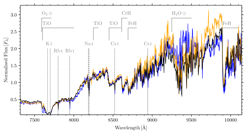
Figure 1: R2500I spectra for J1745$-$1640, normalised at $8100\text{--}8200\,\textup{\AA}$, comparing two independent reduction procedures: PypeIt in black and IRAF in orange. In blue, the heliocentric corrected MagE spectra (2015ApJS..220...18B) for the same object is shown (which is not telluric corrected). The Earth symbol indicates the telluric bands present in the spectra.

4 Analysis

Here, we discuss the analysis of the reduced spectra, in order to produce spectral types, astrophysical parameters and kinematics. We discuss our measurements of astrophysical parameters first because the cross-correlation technique used to measure RV requires the use of a best-fitting model derived template, obtained from the best fit of astrophysical parameters. The code used for both estimating astrophysical parameters and calculating RV is rvfitter (Cooper_rvfitter_2022). This program was developed to effectively recreate in python older codes (e.g. IRAF.Fxcorr, IRAF.Splot, IDL.gaussfit) designed for allowing a user to manually cross-correlate spectra and fit line centres with different profiles. All wavelengths discussed in this Section are in standard air, hence we converted our PypeIt spectra from vacuum to air. This was performed via the specutils package, using the corrections by 1953JOSA...43..339E.

4.1 Spectral typing

We spectral typed both the R300R and R2500I spectra using the classifyTemplate method of the kastredux (kastredux) package. This compared each spectrum against SDSS standards (2007AJ....133..531B; 2010AJ....139.1808S; 2017ApJS..230...16K), from M0–T0, and selected the spectral type with the minimum difference in scaled fluxes ($\Delta F$: equations (3 - 4)) with equally weighted ($W$) points.

$$\Delta F=\sum\frac{W(F_{\mathrm{object}}-KF_{\mathrm{standard}})^{2}}{\sigma_{\mathrm{object}}^{2}}$$ (3)

$$\left.K=\sum\frac{WF_{\mathrm{object}}F_{\mathrm{standard}}}{\sigma_{\mathrm{object}}^{2}}\middle/\right.\sum\frac{WF_{\mathrm{standard}}F_{\mathrm{standard}}}{\sigma_{\mathrm{object}}^{2}}$$ (4)

The spectra had all been smoothed in wavelength with a Gaussian $5\sigma$ kernel, and we only compared the regions from $8000$ to $8500\,\textup{\AA}$ for R2500I and $7000$ to $8000\,\textup{\AA}$ for R300R. This was decided through experimentation, which deliberately excluded regions with telluric features, as those features can cause poorer solutions. Each object was also visually checked against known standards (1999ApJ...519..802K), the spectral sub-types by which we refer to as ‘by eye’. Any spectra with indicators of youth are given optical gravity classes as defined by 2009AJ....137.3345C, from $\beta,\gamma,\delta$ in order of decreasing surface gravity. The kastredux spectral types were our adopted spectral types.

4.1.1 GTC spectral sequence

The 46 spectra from the R2500I VPHG, ordered by our adopted spectral type, are shown in Figures 2 and 3. All spectra are heliocentric corrected, such that the relative motion of the Earth has been removed. Each spectrum shown had an outlier masking routine applied such that points within a rolling ${\approx}15\,\textup{\AA}$ (ten data points) chunk are removed if they had a difference greater than the standard deviation from the median. Additionally, some objects had problematic O${}_{2}$ A-band tellurics. In those cases, we interpolated over the region $7540\text{--}7630\,\textup{\AA}$ from the maximum of the first ${\approx}7.5\,\textup{\AA}$ to minimum of the last ${\approx}7.5\,\textup{\AA}$. Where appropriate, spectra were co-added. All spectra appear noisy in the primary H${}_{2}$O band of ${\approx}9200\text{--}9600\,\textup{\AA}$. The 17 heliocentric corrected, reduced spectra from the R300R grism are shown in Figure 4. The R300R spectra were trimmed from $6500<\lambda<9000\,\textup{\AA}$ due to (a) the lack of signal in the blue regime and (b) to constrain to purely the first order light. Unlike the R2500I spectra, the R300R spectra were not telluric corrected.

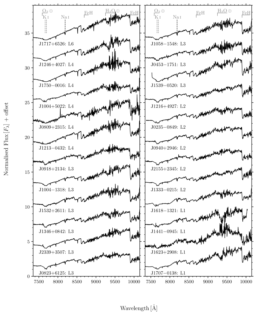
Figure 2: The first 24 of the R2500I VPHG spectra with a linear offset applied, sorted by spectral sub-type. We show the short names and the spectral sub-types from this work, attached to each spectrum. At the top of the figure are grey lines denoting a selection of spectral features typical to L dwarfs, plus the two main telluric bands.

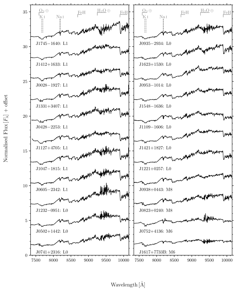
Figure 3: Same as Figure 2 but for the second half of the R2500I VPHG sample.

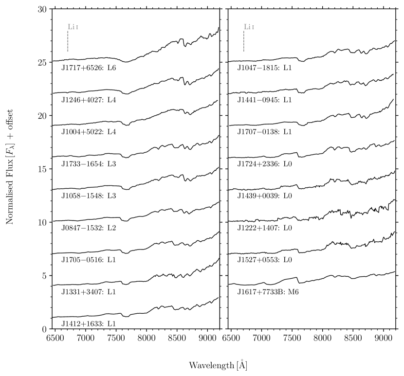
Figure 4: Same as Figure 2 but for the R300R grism spectra. Instead of the spectral features visible in Figures 2 and 3, we only show where any lithium detection would be.

4.2 Fundamental astrophysical parameters

We used the rvfitter.crosscorrelate code on our R300R and R2500I spectra with BT-Settl CIFIST model grids from $1200\leq T_{\mathrm{eff}}\leq 4000$ K and $4.5\leq\log g\leq 5.5$ dex (2011ASPC..448...91A). Lower surface gravity grids were available but not routinely used as the focus was on RV measurement with an a priori expectation of field surface gravity, ${\approx}5$ dex. These models assume a solar metallicity with no variation and are linearly dispersed in steps of $100$ K and $0.5$ dex. This code allowed us to visually select the best fitting model from the array of model grids and for each spectral line from Table 2.

Line	$\lambda$ [Å]
K i-a	7664.8991
K i-b	7698.9646
Rb i-a	7800.268
Rb i-b	7947.603
Na i-a	8183.2556
Na i-b	8194.824
Cs i-a	8521.13165
Cs i-b	8943.47424

Table 2: The list of atomic alkali metal lines used when estimating astrophysical parameters and calculating radial velocities. Wavelengths are as measured by nistdb and are defined in standard air.

We used these chosen lines rather than correlating against the entire model because the models do not exactly match the flux profile of ground based spectra. It was also known that the BT-Settl grids were generated using a different line list to our selected alkali lines, taken from the NIST database (nistdb). For efficiency purposes, each model when being loaded into the code, was interpolated onto the wavelength array of the object being compared against. The models could optionally be Gaussian smoothed, which was helpful for fitting any ‘messy’ regions of models (e.g. telluric bands in models with $T_{\mathrm{eff}}\ \gtrapprox 2000$ K). We normalised the model and data by their respective medians in a given variably sized ‘chunk’ around each spectral line. We noted that around certain lines, particular models appeared almost identical to each other, e.g. around 7000–8000 Å, the $1900$ and $2000$ K models are not visually distinct. This means there is a higher uncertainty for effective temperatures within the 1900–2000 K region. Not every spectral line was used for each object as some have poorly resolved features or low signal-to-noise. Our selected $T_{\mathrm{eff}}$ was the mean $T_{\mathrm{eff}}$ from each line measurement, as was $\log g$. To determine the error on each $T_{\mathrm{eff}}$ and $\log g$ final value, we chose to use the standard deviation from each independent line fit divided by square root of the number of lines used. This error was added in quadrature with half of the separation between each grid, i.e. $50$ K for $T_{\mathrm{eff}}$ and $0.25$ dex for $\log g$.

Additionally, we created an ‘expected’ effective temperature, $\widehat{T_{\mathrm{eff}}}$, using the Filippazzo, sixth order field $T_{\mathrm{eff}}$ relation (2015ApJ...810..158F) and our adopted spectral types. The errors on $\widehat{T_{\mathrm{eff}}}$ correspond with the mean difference in $T_{\mathrm{eff}}$ across $\pm 0.5$ spectral sub-types (our spectral sub-type uncertainty), plus the quoted relation RMS of 113 K.

4.3 Calculating the radial velocities

Only our R2500I spectra were used to determine RVs as the features in R300R spectra are mostly blended/unresolved. We used two methods by which to measure an adopted RV: line centre fitting and cross correlation. We note that our seeing (Table LABEL:table:obslog, corrected for airmass) was almost always smaller than the slit width, which affects the RV offset as the slit is not fully illuminated. The full width at half-maximum was typically 3–4 pixels, corresponding to ${\approx}0.75\text{--}1$ arcseconds. Most observations were seeing-limited, whilst a few, taken in poorer conditions, were slit-limited. The following methods were performed only on heliocentric corrected spectra, hence any quoted RV values are heliocentric corrected.

4.3.1 Line centre fitting

Using the same atomic absorption lines listed in Table 2, we applied the rvfitter.linecentering code to interactively fit Gaussian, Lorentzian and Voigt profiles with the minimum possible width. This minimum possible width is equal to the number of free parameters plus one (although this does not guarantee a successful fit). We used these different profiles to obtain the best fit for a particular line given its underlying absorption characteristics and the available signal-to-noise of the spectral region. The fitting technique used was least-mean-square minimisation. For each spectral line, we subtracted a linear continuum from the data. The continuum corresponds to the medians of selected regions to the blueward and redward sides of the spectral line. Each continuum region is chosen to follow the shape of the spectra with a minimum width of ${\approx}50\,\textup{\AA}$ within 100–200 Å of the spectral line. Also shown during the fitting routine is a fifth order spline, as a visual aid; the minima of the spline does not necessarily correspond to the line position. A example of this routine is given for J1745$-$1640 in Figure 5. The fits were only accepted if they appeared to accurately represent the spectral lines profile upon visual inspection. In general, the most consistently reliable lines were the rubidium lines, sodium doublet and first caesium line. The potassium doublet often was affected by rotational broadening whilst the second caesium line was often affected by neighbouring features. The uncertainty for each line, was the value in the diagonal of the covariance matrix corresponding to centroid position from the least-squares fit, plus the wavelength calibration RMS for that object, Doppler shifted into RV space.

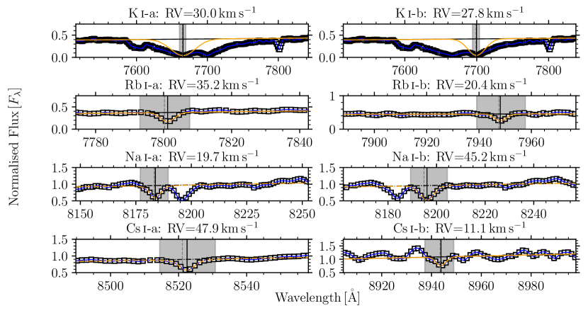
Figure 5: J1745$-$1640 RV calculation via different line profiles (orange: solid – Gaussian; dash-dot – Voigt) against the data (black squares) and fifth order spline fit (blue) in the regime around the eight listed line centres. The flux uncertainty is smaller than the height of each square. The shift from the laboratory line position (vertical dashed grey line) is shown as the vertical solid black line. The horizonal black line (solid or dash-dot, depending on the fitted line profile as above) is the continuum, as is subtracted from the data. A grey band is given, corresponding to the region of data the line profiles are fitted to. The shown region is between the inner edges of the continuum regions.

After measuring every line, we then calculated the overall weighted mean ($\mu_{\text{LC}}$) and weighted standard deviation ($\sigma_{\text{LC}}$), the weights were the inverse of the uncertainties of each line used, squared. The uncertainty from the vacuum to air conversion was negligible (${\ll}0.1$ $\mathrm{km\,s}^{-1}$) compared to the fitting uncertainties calculated from the eight (or less, if rejected) aforementioned lines. The final line centre RV standard error was the weighted standard deviation divided by the square root of the number of lines fit.

4.3.2 Cross-correlation

In addition to estimating the astrophysical parameters with rvfitter.crosscorrelate in Section $\S$4.2, we also used the same package to measure RV by manually shifting the best fitting BT-Settl model as a template. No smoothing was applied to the model template to match the spectral resolution of the object spectrum. This was because smoothing could confuse where the centroid of a line was, when looking by-eye. Likewise, there was no continuum subtraction applied to the object spectrum. The RV shift was in steps of $5,\ 10,\ 100$ $\mathrm{km\,s}^{-1}$, which in turn defined the RV uncertainty on each line ($2.5,\ 5,\ 50$ $\mathrm{km\,s}^{-1}$, i.e. the margin of error). These RV errors are added to the wavelength calibration RMS for the given object (Doppler shifted into an RV error). Not all atomic lines were always used, only in the cases where the model appeared to closely match the apparent line profile. The typical technique was to select a broad region ($\Delta\lambda=100\text{--}200\,\textup{\AA}$) around each spectral line, find the best fitting template in terms of $T_{\mathrm{eff}}$ and $\log g$, then narrow that region ($\Delta\lambda\approx 50\,\textup{\AA}$) to then find an RV. This was a predominantly by-eye technique, although root-mean-square deviation divided by interquartile range (RMSDIQR) values were computed as a numerical guide when comparing models. We also show a fifth order spline, as with the line centering method, as a visual aid. This initial broad region is shown for J1745$-$1640 in Figure 6.

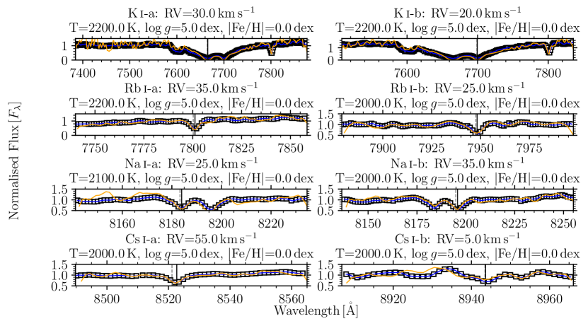
Figure 6: J1745$-$1640 RV calculation via the manually shifted BT-Settl model (orange) against the data (black squares) and fifth order spline fit (blue). The flux uncertainty is smaller than the height of each square. The laboratory line position (vertical dashed grey line) has been manually shifted by the RV given on the sub-plot title (vertical solid black line). Effective temperature, gravity and metallicity are also indicated on each features title.

As in Section $\S$4.3.1, the overall cross-correlated weighted mean RV value ($\mu_{\text{XC}}$) and weighted standard deviation ($\sigma_{\text{XC}}$) was calculated using all of the manually selected lines. We used the same method to estimate the uncertainty in final cross-correlation derived RVs as for the line centre results, by finding the standard error of the mean.

4.3.3 Adopted RV

We created an adopted RV by constructing a weighted mean, using the deviation in each method as the weighting. The different RV values for each line, method and the corresponding probability distribution functions (PDFs) are shown in Figure 7, for J1745$-$1640. We also note that our final adopted RV for J1745$-$1640 obtained from combining the results of the two measurement techniques ($32.7\pm 6.5$ $\mathrm{km\,s}^{-1}$) is in agreement with the values obtained from both the customised IRAF reduced data and the value reported by 2015ApJS..220...18B, within their respective uncertainties. See Appendix LABEL:subsubsec:meth_val for a full description.

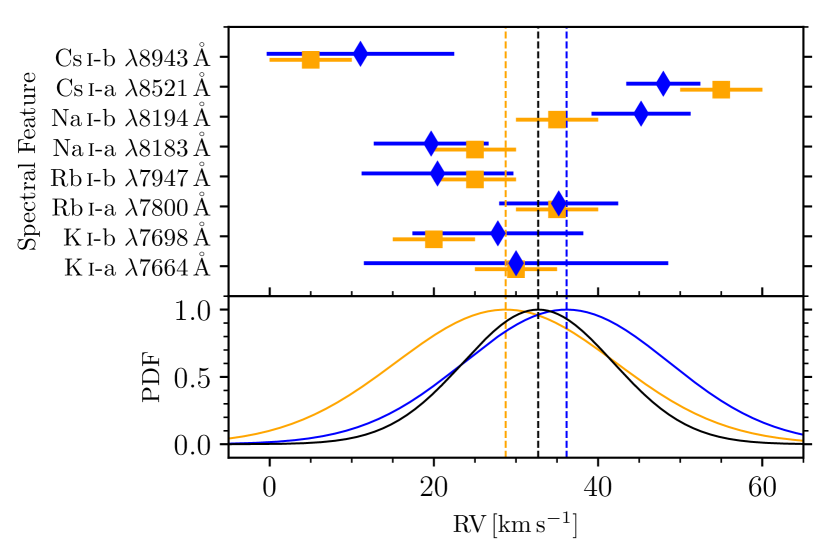
Figure 7: J1745$-$1640 RV values for each given line. In the top panel, orange squares are cross-correlated RVs, blue diamonds are line centre RVs; each spectral feature has been indicated on the $y$ axis. In the bottom panel, the orange curve is the cross-correlated PDF; the blue curve is the line centre PDF; and the black curve is the adopted PDF. The dotted vertical lines are the mean RV values as associated with each PDF.

The adopted RV was the mean ($\mu_{\text{RV}}$) whilst the standard error ($\delta_{\text{RV}}$) was equal to the standard deviation ($\sigma_{\text{RV}}$) divided by $\sqrt{2}$. The mean and standard deviation was calculated through the inverse variance weighting equations (5 and 6). Typically, we found that the cross-correlation technique was more precise (being more controlled by-eye) and robust. The line centre fitting was often more accurate, however, and performed best on the higher quality spectra.

$$\mu_{\text{RV}}=\frac{\mu_{\text{LC}}\sigma_{\text{XC}}^{2}+\mu_{\text{XC}}\sigma_{\text{LC}}^{2}}{\sigma_{\text{LC}}^{2}+\sigma_{\text{XC}}^{2}}$$ (5)

$$\sigma_{\text{RV}}=\sqrt{\frac{\sigma_{\text{LC}}^{2}\sigma_{\text{XC}}^{2}}{\sigma_{\text{LC}}^{2}+\sigma_{\text{XC}}^{2}}}$$ (6)

4.4 Kinematics

Galactic UVW velocities were calculated using our adopted RVs plus Gaia astrometric measurements, using the equations from astrolibpy. We corrected for the Local Standard of Rest (LSR) using the values from 2011MNRAS.412.1237C where U, V, W = ($-8.50,+13.38,+6.49$) $\mathrm{km\,s}^{-1}$. These equations follow the work by 1987AJ.....93..864J, except that U is orientated towards the Galactic anti-centre. We also used BANYAN $\Sigma$ (2015ApJS..219...33G; 2018ApJ...856...23G), which provided moving group classification with associated probability. When using BANYAN $\Sigma$, we checked the resultant probabilities both with and without RV. This was because RV has by far the lowest precision, thus could reduce a likely membership candidate into a field object in error. Our final values are the ones which include RV. Notably, when using velocities in the Galactic reference frame, one can select a Galactic component with $V_{\text{total}}$ (where $V_{\text{total}}$ is the total space velocity, $V_{\text{total}}=\sqrt{U^{2}+V^{2}+W^{2}}$). We followed the work by 2010A&A...511L..10N and define thick disc and halo objects as having $V_{\text{total}}>70\,\mathrm{km\,s}^{-1}$ and $V_{\text{total}}>180\,\mathrm{km\,s}^{-1}$ respectively. This definition, especially for separating the thin and thick disc, is indicative of metallicity; see the Besançon Galaxy models (2014A&A...564A.102C; 2021A&A...654A..13L).

5 Results

In this Section, we present the spectral types, radial velocities and astrophysical parameters. In Table LABEL:table:photometry, we provide photometry from the Gaia, 2MASS and ALLWISE catalogues. We discuss individually interesting objects and objects where our measured results differ significantly from published values.

5.1 Spectral types

In Table 3 we list published spectral types based on optical spectra, near-infrared spectra and the ‘by eye’ and kastredux methods discussed in Section $\S$4.1. This work has produced the first spectral type estimates for six of the 53 objects.

Table 3: Our spectral types compared with the literature optical and near-infrared types for each object.

Object	Lit Opt	Lit NIR	By eye	kastredux	Object	Lit Opt	Lit NIR	By eye	kastredux
short name	sp. type	sp. type	sp. type	sp. type	short name	sp. type	sp. type	sp. type	sp. type
J0028$-$1927	L0:1	L0.52	L0.5	L1	J0235$-$0849	L23	L2:2	L2	L2
J0428$-$2253	L0.54	L02	L0.5	L1	J0453$-$1751	L3:5	L32	L3$\beta$	L3
J0502$+$1442	L06	M92	M9$\beta$	L0	J0605$-$2342	L0:7	L1:2	L0.5	L1
J0741$+$2316	L18	…	L0	L0	J0752$+$4136	M79	…	M6	M6
J0809$+$2315	…	…	L4:	L4	J0823$+$0240	…	…	M9	M8
J0823$+$6125	L2:1	L2.52	L3	L3	J0847$-$1532	L25	…	L2	L2
J0918$+$2134	L2.510	L2.52	L3	L3	J0935$-$2934	L01	L0.52	L0	L0
J0938$+$0443	L06	M82	M9	M8	J0940$+$2946	L16	L0.52	…	L2
J0953$-$1014	L07	M9.52	M9.5$\beta$	L0	J1004$+$5022	L3Vl-G11	L3Int-G12	L3$\beta$	L4
J1004$-$1318	L013	L1:14	L3.5$\beta$	L3	J1047$-$1815	L2.515	L0.52	L1	L1
J1058$-$1548	L310	L316	L3$\beta$	L3	J1109$-$1606	L06	…	L1	L0
J1127$+$4705	L16	…	L1	L1	J1213$-$0432	L55	L42	L5$\beta$	L4
J1216$+$4927	L16	…	L2:	L2	J1221$+$0257	L0.517	M9p18	M9.5	L0
J1222$+$1407	M98	…	M9::	L0	J1232$-$0951	L01	M9.52	M9.5	L0
J1246$+$4027	L419	L42	L4 w/ Li	L4	J1331$+$3407	L01	L1p(red)20	L0	L1
J1333$-$0215	L36	L22	…	L2	J1346$+$0842	L26	…	L2.5	L3
J1412$+$1633	L0.519	L02	L0	L1	J1421$+$1827	L01	M92	M9.5	L0
J1439$+$0039	…	…	…	L0	J1441$-$0945	L0.511	L0.52	L0.5	L1
J1527$+$0553	…	…	…	L0	J1532$+$2611	L16	…	…	L3
J1539$-$0520	L4:11	L221	L4.5	L3	J1548$-$1636	…	L2:22	M9.5	L0
J1617$+$7733B	…	…	…	M6	J1618$-$1321	L0:11	M9.52	L0	L1
J1623$+$1530	L06	…	M9	L0	J1623$+$2908	L16	…	L1::	L1
J1705$-$0516	L0.51	L112	L1	L1	J1707$-$0138	L0.513	L223	L1	L1
J1717$+$6526	L43	L62	L6	L5	J1724$+$2336	…	…	…	L0
J1733$-$1654	L0.5:24	L12	L2	L3	J1745$-$1640	L1.5:24	L1.52	L1	L1
J1750$-$0016	…	L5.522	L5.5	L4	J2155$+$2345	…	L220	L3	L2
J2339$+$3507	L3.51	…	L3.5	L3

Literature Spectral Types: 1.  2008AJ....136.1290R, 2.  2014ApJ...794..143B, 3.  2002AJ....123.3409H, 4.  2003A&A...403..929K, 5.  2003AJ....126.2421C, 6.  2010AJ....139.1808S, 7.  2007AJ....133..439C, 8.  2017MNRAS.470.4885M, 9.  2011AJ....141...97W, 10.  1999ApJ...519..802K, 11.  2008ApJ...689.1295K, 12.  2013ApJ...772...79A, 13.  2010A&A...517A..53M, 14.  2013AJ....146..161M, 15.  1999AJ....118.2466M, 16.  2004AJ....127.3553K, 17.  2014AJ....147...34S, 18.  2015ApJS..219...33G, 19.  2000AJ....120..447K, 20.  2010ApJS..190..100K, 21.  2004A&A...416L..17K, 22.  2007A&A...466.1059K, 23.  2011ApJ...735...14P, 24.  2008MNRAS.383..831P.

The ‘:’ after a spectral type indicates uncertainty of $\pm 1$ whilst ‘p’ indicates peculiarity. The surface gravity flag $\beta$ is given when appropriate, and is discussed in Section $\S$LABEL:subsubsec:individuals. The adopted spectral type is the kastredux method, only overwritten where there are gravity flags in the ‘by eye’ method. In addition, J1246$+$4027 has been typed as having a potential Li i detection ($\lambda 6708\,\textup{\AA}$), which can only be seen in the R300R spectra.

The 47 objects with known spectral types have a standard deviation of 0.5 sub-types between the published values and the ‘by eye’/kastredux results, which we adopt as the error on the new spectral sub-types. When the literature values for a given object differ we adopted the optical spectral type. Our spectral types across the two methods are displayed against the adopted literature spectral types in Figure 8.

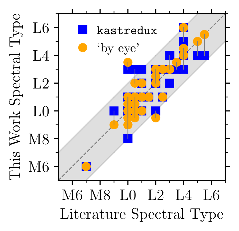
Figure 8: Comparison between this works spectral types and the literature spectral types. Blue squares are spectral types from our adopted, kastredux method whilst orange circles are from the manual ‘by eye’ method. Grey lines connect these two methods and we show a one-to-one dashed grey line with associated $\pm 2$ spectral sub-types confidence bands.

All objects except J1004$-$1318 have sub-type differences between the spectral type derived in this work and the adopted literature spectral type of less than two sub-types. J1004$-$1318, has an optical (Opt) spectral sub-type of L0 (2010A&A...517A..53M) whilst 2013AJ....146..161M found a sub-type of L1 using near-infrared (NIR) spectra; we find a sub-type of L3. However, a more recent study, 2016ApJ...830..144R, found a sub-type of L4 (NIR), which is more consistent with our result. The fit statistic from kastredux is about twice larger for L1 than for L3. In Figure 2, J1004$-$1318 does not seem dissimilar to the neighbouring objects, whereas the L0/L1 spectra appear different (e.g. weaker alkali lines). The different spectral typing of J1004$-$1318 may be due to lower signal-to-noise (S/N) ratios of some observations. For example, 2010A&A...517A..53M exposed for 2400 s at the 2.56 m Nordic Optical Telescope, while we exposed for 1500 s, and with moderately good seeing and low airmass, with a telescope with an aperture over 16 times larger.

5.2 Radial velocity analysis

We have derived RVs for 46 of the observed 53 objects, the seven objects that we did not measure RVs were only observed with the R300R grism. For 20 of the 53 objects, there are published RVs and for 17 of these we have measured RVs. The objects J1004$+$5022, J1441$-$0945 and J1617$+$7733B are candidate members of benchmark systems (Section $\S$2.1), and we adopt the RVs of their primary stars as a comparison with our measured values for the secondary, for a total of 20 comparison RVs. In Figure 9, we plot histograms of the 20 published and the 46 measured values. We also show the difference between the published and measured values of the 20 overlapping objects. If there is more than one literature value, we take the weighted mean RV and standard error on the mean, to compare against the adopted RV from this work. We show literature measurements with respect to their resolutions and define these as: low, $R<2\,500$; mid, $2\,500\leq R\leq 25\,000$; high, $R>25\,000$. The error used to define $\sigma$ are the quadrature summed errors from the literature and our adopted RV.

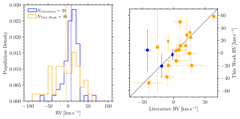
Figure 9: [Left Panel]: Histograms of the RVs calculated in this work (orange) and from the literature (blue) to show the relevant population densities. The dashed vertical lines indicate the means of the associated distributions. [Right Panel]: The RV values from the literature on the $x$ axis with our adopted RV values, on the $y$. We show a one-to-one relation, over which our 20 comparison RVs are plotted. Squares are from low-resolution literature measurements, whereas circles and diamonds are mid- and high-resolution literature measurements respectively. Orange points are like-for-like comparisons and blue points are for the three benchmark systems, i.e., comparisons between our measured secondary RV against the literature RV of the primary.

Our 46 RVs in the heliocentric reference frame are presented in Table 4. This reference frame has been experimented with, in that the heliocentric/barycentric correction via pypeit has been compared with a manual barycentric correction using barycorrpy (2018RNAAS...2....4K). Resultant RV differences from the manual barycentric correction to the pipeline barycentric correction differ by ${\approx}0.1$ $\mathrm{km\,s}^{-1}$. The difference between heliocentric and barycentric correction is $0.5$ $\mathrm{km\,s}^{-1}$ in the case of J1745$-$1640.

Table 4: RVs measured in this work and compared to the literature.

Object	Literature RV	Line Centre RV	Cross Correlation RV	Adopted RV
short name	[kms${}^{-1}$]	[kms${}^{-1}$]	[kms${}^{-1}$]	[kms${}^{-1}$]
J0028$-$1927	…	$18.6\pm 7.7^{\mathrm{11111110}}$	$26.3\pm 13.2^{\mathrm{11111111}}$	$20.4\pm 14.9$
J0235$-$0849	$15.3\pm 11.2\hyperlink{litrvs}{{}^{1}}$, $22.8\pm 6.1\hyperlink{litrvs}{{}^{2}}$	$30.9\pm 27.8^{\mathrm{00110111}}$	$26.7\pm 21.0^{\mathrm{00111111}}$	$28.4\pm 29.1$
J0428$-$2253	…	$69.3\pm 36.3^{\mathrm{11111110}}$	$16.0\pm 6.1^{\mathrm{00011111}}$	$17.0\pm 12.3$
J0453$-$1751	…	$15.1\pm 2.3^{\mathrm{00010110}}$	$13.3\pm 5.9^{\mathrm{00111111}}$	$15.0\pm 8.3$
J0502$+$1442	…	$41.3\pm 5.8^{\mathrm{11101110}}$	$41.2\pm 5.4^{\mathrm{11111111}}$	$41.3\pm 10.7$
J0605$-$2342	…	$23.4\pm 6.3^{\mathrm{00011110}}$	$25.0\pm 8.8^{\mathrm{11111111}}$	$23.7\pm 11.1$
J0741$+$2316	…	$31.1\pm 0.2^{\mathrm{00011000}}$	$38.0\pm 3.3^{\mathrm{11001110}}$	$31.1\pm 7.8$
J0752$+$4136	$8.5\pm 10.1\hyperlink{litrvs}{{}^{1}}$	$-3.0\pm 19.9^{\mathrm{01001100}}$	$14.2\pm 15.7^{\mathrm{11111100}}$	$4.7\pm 19.7$
J0809$+$2315	…	$-48.2\pm 3.2^{\mathrm{00011110}}$	$-38.0\pm 9.5^{\mathrm{00011111}}$	$-47.4\pm 8.9$
J0823$+$0240	…	$-26.6\pm 3.8^{\mathrm{00001110}}$	$-4.3\pm 4.5^{\mathrm{11111110}}$	$-21.4\pm 8.8$
J0823$+$6125	…	$-22.6\pm 11.3^{\mathrm{00011110}}$	$-12.9\pm 12.7^{\mathrm{10111111}}$	$-19.6\pm 15.4$
J0918$+$2134	…	$-92.9\pm 7.3^{\mathrm{00001110}}$	$-80.0\pm 7.5^{\mathrm{00111110}}$	$-88.2\pm 10.6$
J0935$-$2934	…	$-3.7\pm 13.2^{\mathrm{10001110}}$	$-22.5\pm 6.1^{\mathrm{11111111}}$	$-16.9\pm 12.8$
J0938$+$0443	$25.4\pm 13.3\hyperlink{litrvs}{{}^{1}}$	$2.7\pm 7.2^{\mathrm{00011110}}$	$-5.7\pm 6.7^{\mathrm{11111101}}$	$-0.7\pm 11.1$
J0940$+$2946	$27.3\pm 11.8\hyperlink{litrvs}{{}^{1}}$, $4.1\pm 7.1\hyperlink{litrvs}{{}^{2}}$	$51.6\pm 5.1^{\mathrm{00011110}}$	$35.0\pm 9.2^{\mathrm{11111111}}$	$49.4\pm 10.3$
J0953$-$1014	…	$63.2\pm 7.9^{\mathrm{01000011}}$	$10.0\pm 7.5^{\mathrm{11111111}}$	$47.6\pm 11.3$
J1004$+$5022	$-1.7\pm 1.5{}^{†}\text{<span class="ltx\_ref ltx\_ref\_self">litrvs</span>}$