The loop equations for
noncommutative geometries on quivers

Abstract.

We define a path integral over Dirac operators that averages over noncommutative geometries on a fixed graph, as the title reveals, using quiver representations. We prove algebraic relations that are satisfied by the expectation value of the respective observables, computed in terms of integrals over unitary groups, with weights defined by the spectral action. These equations generalise the Makeenko-Migdal equations—the constraints of lattice gauge theory—from lattices to arbitrary graphs. As a perspective, our loop equations are combined with positivity conditions (on a matrix parametrised by composition of Wilson loops). On a simple quiver this combination known as ‘bootstrap’ is fully worked out. The respective partition function boils down to an integral known as Gross-Witten-Wadia model; their solution confirms the solution bootstrapped by our loop equations.

1. Introduction

Before discussing our problem in its due context, we describe it aridly, postponing its motivation for Section 1.1. For integers $N$ and $n$ satisfying $N>n>1$, fix a polynomial $S\in\mathbb{C}_{\langle 2n\rangle}=\mathbb{C}{\langle u_{1},u_{1}^{*},u_{2},u_{2}^{*},\ldots,u_{n},u_{n}^{*}\rangle}$ in noncommutative $u$-variables satisfying $u_{j}u_{j}^{*}=1=u_{j}^{*}u_{j}$ for $j=1,\ldots,n$. Consider a family of integrals of the type

$$I_{\beta}=\int_{\mathrm{U}(N)^{n}}\operatorname{Tr}\beta(U_{1},U^{*}_{1},\ldots,U_{n},U_{n}^{*})\mathrm{e}^{N\operatorname{Tr}S(U_{1},U^{*}_{1},\ldots,U_{n},U_{n}^{*})}{\mathrm{d}}U_{1}{\mathrm{d}}U_{2}\cdots{\mathrm{d}}U_{n},\quad\beta\in\mathbb{C}_{\langle 2n\rangle},$$ (1.1)

with each factor ${\mathrm{d}}U_{i}$ being the Haar measure on $\mathrm{U}(N)$. Assuming that $\operatorname{Tr}S$ is real-valued over the whole integration domain, we derive the loop equations, that is to say, algebraic relations among the integrals $\{I_{\beta}\}_{\beta\in\mathcal{I}}$ parametrised by a certain family $\mathcal{I}\subset\mathbb{C}_{\langle 2n\rangle}$. This type of integrals has been considered by physicists in the context of lattice gauge field theory. In mathematics, integrals over the unitary group are relevant in the context of Weingarten-calculus [Col03], developed mainly by Collins and collaborators (e.g. [CŚ06, CGL24]).

1.1. Motivation: Random matrix theory and noncommutative geometry

Our interest in integrals of the type (1.1) emerges from Connes’ noncommutative geometrical [Conn94] approach to fundamental interactions, in which geometric notions are mainly governed by a self-adjoint operator $D$ named after Dirac. In this setting, the physical action $S(D)$ is claimed to depend only on (the spectrum of) $D$ and is known as spectral action [CC97]. The problem that motivates this article is the evaluation of the moments that the spectral action yields via

$$\mathbb{E}[h(D)]=\frac{1}{\mathcal{Z}}\int_{\text{Dirac}}h(D)\mathrm{e}^{-S(D)}{\mathrm{d}}D,\qquad\mathbb{E}[1]=1,\quad h(D)\in\mathbb{R},$$ (1.2)

for an ensemble of Dirac operators $D$ (the normalisation condition defines $\mathcal{Z}$). Of course, this requires to have defined the measure ${\mathrm{d}}D$ on such ensemble, as well as the ensemble itself. (In the problem originally formulated in [CM08, Sec. 19] the spectral action contains fermions, as it has been recently addressed in [KPV24], but which we do not include here.)

Part of the relatively vivid interest in the problem (1.2) during the last decade is due to the reformulation [Bar15] of fuzzy spaces as finite-dimensional spectral triples. This led to the application of tools related to random matrix theory [AK24, Pér22a, KP21, Pér21, Pér22b, HKPV22] that followed to the first numerical results [BG16]. All these works deal with multimatrix interactions that include a product of traces (as opposed to the ordinary interactions that are a single trace of a noncommutative polynomial).

Independently, in [vS11, Cor. 19] the Taylor expansion of the spectral action yields a hermitian one-matrix model of the form $V(M)=\sum_{l=1}^{\infty}\sum_{i_{1},i_{2},\ldots,i_{l}}F_{i_{1},i_{2},\ldots,i_{l}}M_{i_{1},i_{2}}M_{i_{2},i_{3}}\cdots M_{i_{l},i_{1}}$, with $F_{i_{1},i_{2},\ldots,i_{l}}\in\mathbb{R}$. This series was shown in [vNvS21] to be convergent under certain conditions and, combining some elements of [CC06] with own techniques, to possess a neat reorganisation in terms of a series expansion in universal Chern-Simons forms and Yang-Mills forms integrated against $(B,b)$-cocycles that do depend on the geometry. Each monomial of the model $V(M)$ above breaks unitarity and thus goes beyond the solved generalisations [GHW20, BHGW22] of the Kontsevich matrix model [Kon92] (in which unitary invariance is broken only by the propagator) known as Grosse-Wulkenhaar model [GW14].

These two independent approaches portend a symbiosis between random matrix theory and noncommutative geometry. Both the multiple trace interactions and the unitary-broken interactions could motivate (if they have not yet) new developments in random matrix theory. And vice versa, the path-integral quantisation (1.2) of noncommutative geometries seems hopeless without the intervention of random matrix theory.

1.2. Ensembles of unitary matrices in noncommutative geometry

The interaction between these two disciplines has taken place in hermitian grounds. In this article, integrals over Dirac operators boil down to ensembles of unitary matrices (they are also unitary-invariant, like ordinary hermitian matrix ensembles, but unitary ensembles integrate over unitary random matrices). These can be considered as an approach to average over ‘noncommutative geometries on a graph’. When the graph is provided with additional structure, it might be grasped as a discretisation of space. For instance, edges would carry a representation while vertices equivariant maps; at least so in the spin network approach. Here, we refrain from including information associated to gravitational degrees of freedom and address exclusively the problem of gauge interactions. The background geometry is therefore fixed and the finiteness of the unitary groups appearing is not a shortage of the theory; as a caveat, they are not to be interpreted as a truncation of infinite-dimensional symmetries (but to be compared with the unitary structure group of Yang-Mills, for example).

Representation theory does still play a role, but rather in the context of quiver representations in a certain category that emerges from noncommutative geometry, as exposed in [Pér24] after the pioneering ideas of [MvS14].

We can now restate the aim of this article as follows:

Define a partition function for noncommutative geometries on a graph—that is, define a measure over all ‘compatible’ Dirac operators—and prove algebraic relations that the respective observables shall satisfy. Such quantities have the form $I_{\beta}$ as in eq. (1.1) and are called Wilson loops (although not each $I_{\beta}$ is a Wilson loop on a given graph).

Proper definitions follow in the main text. Such relations generalise the Makeenko-Migdal equations, the loop equations in lattice gauge theory. After introducing the setting in Section 2, we prove the main result in Section 3 and conclude with a fully worked-out application that mixes the loop equations with positivity conditions of a certain matrix (‘bootstrap’) in Section 4.

2. Quiver representations and noncommutative geometry

We call quiver $Q$ a directed multigraph. Since $Q$ is directed, there are maps $s,t:Q_{1}\rightrightarrows Q_{0}$ (from the edge-set $Q_{1}$ to the vertex-set $Q_{0}$) determining the vertex $s(e)$ at which an edge $e$ begins, and the one $t(e)$ where it ends. Multiple edges $e,e^{\prime}\in Q_{1}$ and self-loops $o_{v}\in Q_{0}$ at a certain vertex $v\in Q_{0}$ are allowed, namely $\{s(e),t(e)\}=\{s(e^{\prime}),t(e^{\prime})\}$ as sets, and $s(o_{v})=t(o_{v})=v$, respectively.

One interprets a quiver $Q$ as a category whose objects are $Q_{0}$. The morphisms $\hom_{Q}(v,w)$ are the paths from $v$ to $w$, namely edge-sequences $\gamma=(e_{1}e_{2}\cdots e_{n})$ with $e_{1},\ldots,e_{n}\in Q_{1}$ and $s(\gamma)=s(e_{1})=v$, and $t(\gamma)=t(e_{n})=w$ as well as $t(e_{j})=s(e_{j+1})$ for $j=1,\ldots,n-1$. We shall write $\gamma:v\to w$ if $v=s(\gamma)$ and $w=t(\gamma)$ and call $\ell(\gamma)=n$ the length of $\gamma$. The path $\gamma$ with reversed order is denoted by $\bar{\gamma}=(e_{n}e_{n-1}\cdots e_{2}e_{1})$ (not to be confused with the inverse morphism of $\gamma$). Obviously, unless otherwise stated, paths are directed, but it will prove useful to consider also paths in $\Gamma Q$, the underlying graph of the quiver ($Q$ with forgotten orientations). If $s(\gamma)=t(\gamma)$ we say that a path $\gamma$ is a loop. The space of loops at $v$, is denoted here $\Omega_{v}(Q)$, that is $\Omega_{v}(Q)=\hom_{Q}(v,v)$, and $\Omega Q$ will denote the space $\cup_{v\in{Q_{0}}}\Omega_{v}(Q)$ of all loops.

A quiver exists essentially to be represented (otherwise one would say multidigraph) in a category $\mathcal{C}$. A $\mathcal{C}$-representation of $Q$ is by definition a functor from $Q$ to $\mathcal{C}$.

2.1. The spectral triple associated to a quiver representation

We restrict the discussion to finite dimensions and introduce the setting of [Pér24]. We dedicated Section 2.4 to examples of the new constructions that appear here. By definition, an object in the category ${\mathscr{pS}}$ of prespectral triples is a pair $(A,H)$ of a unital $*$-algebra $A$ faithfully $*$-represented, $\lambda:A\curvearrowright H$, in an inner product $\mathbb{C}$-vector space $H$ ($*$-represented means here, that $\lambda(a^{*})$ is the adjoint operator of $\lambda(a)$ for all $a\in A$). A morphisms in $\hom_{{\mathscr{pS}}}(A_{s},H_{s}\,;\,A_{t},H_{t})$ is a couple $(\phi,U)$ of an involutive unital algebra map $\phi:A_{s}\to A_{t}$ as well as a unitary map $U:H_{s}\to H_{t}$. As part of the definition, a morphism should in addition satisfy $U\lambda_{s}(a)U^{*}=\lambda_{t}[\phi(a)]$ for all $a\in A$.

In other words, a ${\mathscr{pS}}$-representation of $Q$ associates with each vertex $v$ of $Q$ a prespectral triple $(A_{v},H_{v})\in{\mathscr{pS}}$ and with any path $\gamma:v\to w$ a morphism $(\phi_{\gamma},\operatorname{\mathrm{hol}}\gamma):(A_{v},H_{v})\to(A_{w},H_{w})$ in such a way that if $\gamma=(e_{1}\cdots e_{n})$, then $\operatorname{\mathrm{hol}}\gamma=U_{e_{n}}\cdots U_{e_{1}}$ and $\phi_{\gamma}=\phi_{e_{n}}\circ\phi_{e_{n-1}}\circ\cdots\circ\phi_{e_{1}}$, where $\phi_{e_{j}}:A_{s(e_{j})}\to A_{t(e_{j})}$ and $U_{e_{j}}:H_{s(e_{j})}\to H_{t(e_{j})}$ form a ${\mathscr{pS}}$-morphism. We refer to $\operatorname{\mathrm{hol}}\gamma$ as the holonomy of $\gamma$. (If $\gamma$ is not a loop, parallel transport would be the precise term; for sake of notation, we call this ‘holonomy’ too.)

If two vertices are connected by a path $\gamma$, notice that $\operatorname{\mathrm{hol}}\gamma$ is a unitarity and $\dim H_{s(\gamma)}=\dim H_{t(\gamma)}$. If $Q$ is connected, there might be no (directed) path between two given vertices $v$ and $w$; it is however easy—if necessary after inverting some subpaths of a path $\tilde{\gamma}$ in $\Gamma Q$ that connects $v$ with $w$—to establish the constancy of the map $Q_{0}\ni v\mapsto\dim H_{v}:=N$; we call such constant $N=\dim R$, the dimension of the representation $R$, somehow abusively.

A spectral triple $(A,H,D)$ is a prespectral triple $(A,H)$ together with a self-adjoint element $D\in\operatorname{\mathrm{End}}(H)$, referred to as Dirac operator. (This terminology comes from the non-trivial statement that $D$ is the spin geometry Dirac operator [Conn13], if certain operators are added to the [in that case, infinite-dimensional] spectral triple and if, together with $D$, such operators satisfy a meticulous list of axioms; see also [vS15] for an introduction geared to physicists).

Remark 2.1.

As a side note, it is possible to compute the space of all ${\mathscr{pS}}$-representations of $Q$. It was proven in [Pér24] that such space—which in fact forms the category of representations—can be described in terms of products of unitary groups subordinated to combinatorial devices called Bratteli networks (Sec. 2.3). At this point, it is important to observe that, in stark contrast with ordinary $\textsc{Vect}_{\mathbb{C}}$-quiver representations, providing labels to the vertices is not enough to determine a ${\mathscr{pS}}$-quiver representation. The lifts of whole paths should exist, and this requires the compatibility of the maps $\phi_{v}$ at all vertices $v$, which in turn is what the so-called Bratteli networks guarantee (concretely unital $*$-algebra maps for $M_{m}(\mathbb{C})\to M_{n}(\mathbb{C})$ for $m>n$ do not exist, and if a representation yields $A_{s(e)}=M_{m}(\mathbb{C})$ and $A_{t(e)}=M_{n}(\mathbb{C})$ for some edge $e$, a lift fails, cf. [Pér24, Ex. 3.16]). Despite this, we denote representations of quivers as $R=\{(A_{v},H_{v}),(\phi_{e},U_{e})\}_{v\in Q_{0},e\in Q_{1}}$ instead of $R=\{(A_{v},H_{v}),(\phi_{\gamma},\operatorname{\mathrm{hol}}\gamma)\}_{v\in Q_{0},\gamma\in\Omega Q}$, meanwhile under the tacit assumption that lifts of whole paths exist. A characterization follows in next the section.

We associate now a spectral triple to a given ${\mathscr{pS}}$-representation $R=\{(A_{v},H_{v}),(\phi_{e},U_{e})\}_{v\in Q_{0},e\in Q_{1}}$ of a connected quiver $Q$. We define the Dirac operator associated to $R$ as the matrix $D_{Q}(R)\in M_{\#Q_{0}}(\mathbb{C})\otimes M_{N}(\mathbb{C})$ with matrix entries $[D_{Q}(R)]_{v,w}\in M_{N}(\mathbb{C})$ in the second factor given by

$$[D_{Q}(R)]_{v,w}=\bigg{(}\sum_{e\in s^{-1}(v)\cap t^{-1}(w)}U_{e}\bigg{)}+\bigg{(}\sum_{e\in t^{-1}(v)\cap s^{-1}(w)}U_{e}^{*}\bigg{)}\qquad(v,w\in Q_{0}).$$ (2.1)

By construction, this operator is self-adjoint, and crucially for our purposes, the objects form a spectral triple,

$$\big{(}A_{Q}(R),H_{Q}(R),D_{Q}(R)\big{)}=\bigg{(}\bigoplus_{v\in Q_{0}}A_{v},\bigoplus_{v\in Q_{0}}H_{v},D_{Q}(R)\bigg{)}.$$ (2.2)

2.2. The spectral action

Given a polynomial $f(x)=f_{0}+f_{1}x^{1}+f_{2}x^{2}+\ldots+f_{d}x^{d}$ in real variables $f_{0},f_{1},\ldots,f_{d}\in\mathbb{R}$, and a quiver representation, the spectral action on a quiver reads $S(D)=\operatorname{Tr}_{H}f(D)$, where we abbreviate $D=D_{Q}(R)$ and $H=H_{Q}(R)$. It is possible to compute the spectral action as a loop expansion in terms of generalised plaquettes $\gamma$ as follows

$$\operatorname{Tr}_{H}f(D)=\sum_{k=1}^{d}f_{k}\,\sum_{v\in Q_{0}}\,\,\sum_{\begin{subarray}{c}\gamma\in\Omega_{v}(Q)\\ \ell(\gamma)=k\end{subarray}}\operatorname{Tr}\operatorname{\mathrm{hol}}\gamma,$$ (2.3)

where $\operatorname{Tr}$ in the rhs is the trace of $M_{N}(\mathbb{C})$ with $\operatorname{Tr}1=\dim R=N$. The proof of eq. (2.3) is given in [Pér24], but the reader will recognise this formula as a noncommutative generalisation of the following well-known fact in graph theory: if $C_{G}$ denotes the adjacency matrix of a graph $G$, then the number of length-$n$ paths in $G$ between two of its vertices, $i$ and $j$, is the entry $[C_{G}^{n}]_{i,j}$ of the matrix $(C_{G})^{n}$.

2.3. The measure on the space of Dirac operators and the partition function

Now we break down the space of ${\mathscr{pS}}$-representations of $Q$,

$$\operatorname{\mathrm{Rep}_{{\mathscr{pS}}}}(Q):=[Q,{\mathscr{pS}}]=\{\text{functors }Q\to{\mathscr{pS}}\}.$$ (2.4)

Let $A_{v}=\oplus_{j=1}^{l_{v}}M_{n_{v,j}}(\mathbb{C})$ denote the algebra associated by $R$ to the vertex $v$ (so $l_{v}$ is the number of simple subalgebras of $A_{v}$). Let $r_{v,j}$ be the multiplicity of the action of the factor $M_{n_{v,j}}(\mathbb{C})\subset A_{v}$ on the Hilbert space $H_{v}$, that is $H_{v}=\oplus_{j=1}^{l_{v}}\mathbb{C}^{r_{v,j}}\otimes\mathbb{C}^{n_{v,j}}$ where $M_{n_{v,j}}(\mathbb{C})$ only acts non-trivially on $\mathbb{C}^{n_{v,j}}$ via the fundamental representation. These integers are not arbitrary, since clearly the totality of the $\{n_{v,1},\ldots,n_{v,l_{v}}\}_{v}$ should be such that unital $*$-algebra maps between vertices connected by an edge exist. The next definition, reformulated from [Pér24], captures this requirements.

Definition 2.2.

A Bratteli network $B$ on a connected quiver $Q$ consists of the following data:

1. an integer $l_{v}>0$ for each vertex $v\in Q_{0}$

2. a $l_{v}$-tuple $\mathbf{r}_{v}\in\mathbb{Z}_{>0}^{l_{v}}$ for each vertex

3. another $l_{v}$-tuple $\mathbf{n}_{v}\in\mathbb{Z}_{>0}^{l_{v}}$for each $v\in Q_{0}$

4. for each edge $e\in Q_{1}$, a matrix $C_{e}\in M_{l_{s(e)}\times l_{t(e)}}(\mathbb{Z}_{\geq 0})$ such that

   $$\mathbf{r}_{s(e)}=C_{e}\mathbf{r}_{t(e)}\quad\text{ and }\quad\mathbf{n}_{t(e)}=C^{\text{\tiny{$\mathrm{T}$}}}_{e}\mathbf{n}_{s(e)}.$$ (2.5)

For sake of notation, we denote Bratteli networks with the variables $B$ or $(\mathbf{n},\mathbf{r})$ leaving the rest of data implicit. If $\langle\mathbf{a},\mathbf{b}\rangle=\sum_{i}a_{i}b_{i}$ is the standard bilinear form on $\mathbb{Z}^{\infty}\times\mathbb{Z}^{\infty}$, it is essential to observe that Conditions (2.5) guarantee that

$$\langle\mathbf{n}_{s(e)},\mathbf{r}_{s(e)}\rangle=\langle\mathbf{n}_{s(e)},C^{\text{\tiny{$\mathrm{T}$}}}_{e}\mathbf{r}_{t(e)}\rangle=\langle C_{e}\mathbf{n}_{s(e)},\mathbf{r}_{t(e)}\rangle=\langle\mathbf{n}_{t(e)},\mathbf{r}_{t(e)}\rangle,\qquad e\in Q_{1},$$ (2.6)

is a constant integer $N$, whenever a quiver is connected. A representation determines a Bratteli network by inserting the integer variables of the first paragraph of this subsection into Def. 2.2 (notations coincide on purpose, and $N$ is the dimension of the representation).

The next question arises:

what is missing a Bratteli network $B$ in order to determine a quiver ${\mathscr{pS}}$-representation?

In the light of the spectral triple $(\oplus_{v\in Q_{0}}A_{v},\oplus_{v\in Q_{0}}H_{v},D_{Q}(R))$ that is associated to a quiver representation, since a Bratteli network is equivalent to the first pair of objects, $(\oplus_{v\in Q_{0}}A_{v},\oplus_{v\in Q_{0}}H_{v})$, the relevant answer is that the missing piece is the Dirac operator associated to the quiver. They exist in abundance and we are interested in their probability distribution.

Definition 2.3.

Given a Bratteli network $B=\{A_{v},H_{v}\}_{v\in Q_{0}}$ on a connected quiver $Q$, the space of Dirac operators $\operatorname{\mathscr{D}}({B})$ is defined as the set of ${\mathscr{pS}}$-maps between vertices

$$D=\big{\{}(\phi_{e},U_{e})\in\hom_{\mathscr{pS}}(A_{s(e)},H_{s(e)}\,;\,\,A_{t(e)},H_{t(e)})\big{\}}_{e\in Q_{1}}$$ (2.7)

that complete $B$ and make it a ${\mathscr{pS}}$-representation of $Q$, that is

$$\operatorname{\mathscr{D}}({B}):=\{\,D\text{ as in }\eqref{C}\mid\,(B,D)\in\operatorname{\mathrm{Rep}_{{\mathscr{pS}}}}(Q)\}.$$

Once labels to the vertices are consistently assigned by the Bratteli network $B$, the possible labels of an edge $e$ are parametrised by $\prod_{j=1,\ldots,l_{t(e)}}\mathrm{U}(n_{t(e),j})$ [Pér24, Lemma 3.5]. Therefore

$$\operatorname{\mathscr{D}}({B})=\coprod_{e\in Q_{1}}\prod_{j=1,\ldots,l_{t(e)}}\mathrm{U}(n_{t(e),j}).$$

The overlapping notation was then on purpose, as $D\in\operatorname{\mathscr{D}}({B})$, and $D_{Q}(R)$ as the Dirac operator of the spectral triple associated to a quiver ${\mathscr{pS}}$-representation, entail the same information. This in turn motivates the following measure.

Definition 2.4.

Given a Bratteli network $B$ on a connected quiver $Q$, we define the Dirac operator measure ${\mathrm{d}}D$ on the space of Dirac operators $\operatorname{\mathscr{D}}(B)$ by

$${\mathrm{d}}D:=\prod_{(v,w)\in Q_{0}\times Q_{0}}{\mathrm{d}}[D_{Q}(R)]_{v,w},\quad\text{ where }\quad{\mathrm{d}}[D_{Q}(R)]_{v,w}:=\prod_{e\in s^{-1}(v)\cap t^{-1}(w)}\prod_{j=1}^{l_{t(e)}}{\mathrm{d}}u_{e,j},$$ (2.8)

being ${\mathrm{d}}u_{e,j}$ the Haar measure on $\mathrm{U}({{n_{t(e),j}}})$, where $u_{e,j}$ sits in the matrix $U_{e}$ associated to $e$ by $R$ in the respective block-diagonal entry in

$$U_{e}=\operatorname{\mathrm{diag}}(1_{r_{t(e),1}}\otimes u_{e,1},1_{r_{t(e),2}}\otimes u_{e,2},\ldots,1_{r_{t(e),l_{t(e)}}}\otimes u_{e,l_{t(e)}}).$$ (2.9)

Definition 2.5.

Given a Bratteli network $B$ on a quiver $Q$, the partition function reads

$$\mathcal{Z}_{Q,B}(f)=\int_{\operatorname{\mathscr{D}}(B)}\mathrm{e}^{-N\operatorname{Tr}_{H}f(D)}{\mathrm{d}}D,\qquad$$ (2.10)

where $D\in\operatorname{\mathscr{D}}(B)$ complements the initial Bratteli network making of it a representation $R=(B,D)$ of dimension $\dim R=N$ given by the integer (2.6). In the Boltzmann weight, the spectral action $\operatorname{Tr}_{H}f(D)$ is given by eq. (2.3).

Remark 2.6.

Some remarks related to the meaning of the partition function:

1. The Dirac operator measure ${\mathrm{d}}D$ is the product Haar measure on $\prod_{e\in Q_{1}}\prod_{i=1}^{l_{t(e)}}\mathrm{U}({{n_{t(e),i}}})\hookrightarrow\mathrm{U}(N)^{\#Q_{1}}$ since $\langle\mathbf{n}_{v},\mathbf{r}_{v}\rangle=\sum_{i=1,\ldots,l_{v}}r_{v,j}\times n_{{v,i}}=N$ holds at each vertex, by eq. (2.6).

2. In the gauge theory picture, $Q$ is a coarse set of data for the base manifold (of a principal bundle). A Bratteli network on $Q$ predetermines a ‘local field of gauge groups’, that is $Q_{0}\ni v\mapsto\mathcal{U}(A_{v})$. The holonomies of paths will therefore gather unitarities that can be multiplied thanks to the embedding (2.9). It would be interesting to explore whether the present structures relate to lifts of Krajewski diagrams (that classify finite spectral triples [Kra98, PS98]) in the sense of [MN23] in some special cases of one or both theories.

3. Due to (2) of this remark and because of the previous identification of a Bratteli network $B$ with fixed data $(A_{Q}(R),H_{Q}(R),\,\raisebox{1.9pt}{\text{$\bullet$\hskip 0.7pt}}\,)$ of the spectral triple in (2.2), if $S(D)$ the spectral action (2.3), the partition function in (2.10) is of the form

   $$\mathcal{Z}_{A_{Q},H_{Q}}(f)=\int_{\begin{subarray}{c}\phantom{nix}\\ D\text{ makes }(A_{Q},H_{Q},D)\\ \text{into a spectral triple}\end{subarray}}\mathrm{e}^{-NS(D)}{\mathrm{d}}D.$$ (2.11)

4. According to the definition of $D_{Q}(R)$ in eq. (2.1), the Dirac operators’ entries determine self-adjoint matrices $\mathsf{A}_{e}\in(A_{t(e)})_{{}_{\text{\tiny s.a.}}}$, interpreted as connections, given by $\mathsf{A}_{e}=\operatorname{\mathrm{diag}}(\mathsf{a}_{e,1},\mathsf{a}_{e,2},\ldots,\mathsf{a}_{e,l_{t(e)}})$ along the edges by $u_{e,i}=:\exp(\sqrt{-1}\mathsf{a}_{e,i})$ for $i=1,\ldots,l_{t(e)}$, cf. eqs (2.9).

5. For fixed $N$, the partition function $\mathcal{Z}_{Q}=\sum_{R\text{ ${\mathscr{pS}}$-rep of $Q$}}^{\dim R=N}\mathcal{Z}_{Q,R}$ is also an interesting quantity, or even more so the sum over a class of quivers $Q$ encoding different background geometries, $\mathcal{Z}=\sum_{Q}\sum_{R\text{ ${\mathscr{pS}}$-rep of $Q$}}^{\dim R=N}\mathcal{Z}_{Q,R}$. For the moment we content ourselves with the partition function (2.10) for a fixed Bratteli network $B$ and a fixed quiver $Q$.

Definition 2.7.

For any $\beta\in\Omega(\Gamma Q)$, a Wilson loop is by definition

$$\mathbb{E}[\operatorname{Tr}(\operatorname{\mathrm{hol}}\beta)]:=\frac{1}{\mathcal{Z}_{Q,B}}\int_{\operatorname{\mathscr{D}}(B)}\operatorname{Tr}\operatorname{\mathrm{hol}}(\beta)\mathrm{e}^{-NS(D)}{\mathrm{d}}D.$$

2.4. Illustrating the previous section

Let us pick an example quiver $Q={\includegraphics[width=34.44434pt]{quiver_HCIZ}}$, whose self-loops are denoted by $o$-variables, as before. The concepts introduced the last subsection are exemplified in the following list.

1. Bratteli network, Def. 2.2. On $Q$ as above, an example of data of a Bratteli network is

   $$l_{v} =2 l_{w} =1 C_{e} =(2,1)^{\text{\tiny{$\mathrm{T}$}}}$$

   $$\mathbf{n}_{v} =(2,3)^{\text{\tiny{$\mathrm{T}$}}} \mathbf{n}_{w} =8 C_{o_{v}} =\operatorname{\mathrm{diag}}(1,1)$$

   $$\mathbf{r}_{v} =(4,2)^{\text{\tiny{$\mathrm{T}$}}} \mathbf{r}_{w} =2 C_{o_{w}} =1.$$

2. Why is $B$ a Bratteli ‘network’? In the illustration an integer $n$ in a green (or circular) nodes over a vertex represents the simple algebra $M_{n}(\mathbb{C})$. The whole algebra associated to the vertex is the sum over all green circles above it. Inside gray rectangles the Hilbert spaces acted on by each simple subalgebra are represented; the non-trivial action takes place only on the second factor.

   $$H_{v} =(\mathbb{C}^{4}\otimes\mathbb{C}^{3})\oplus(\mathbb{C}^{2}\otimes\mathbb{C}^{2})$$

   $$A_{v} =M_{3}(\mathbb{C})\oplus M_{2}(\mathbb{C})$$

   $$H_{w} =\mathbb{C}^{2}\otimes\mathbb{C}^{8}$$

   $$A_{w} =M_{8}(\mathbb{C})$$

   The network arises when all the lines that $\{C_{e}\}_{e\in Q_{1}}$ represent are composed. The $C$-matrices associated to the self-loops are the identity and therefore not worth depicting. Each unital $*$-algebra map is given by block embeddings of the simple algebras into the target algebra (up to unitary conjugations that parametrise the space of Dirac $\operatorname{\mathscr{D}}(B)$ operators for $B$ below). The entry $(C_{e})_{i,j}\in\mathbb{Z}_{\geq 0}$ represents how many blocks from the $i$-th factor of $A_{s(e)}$ are embedded into the $j$-th factor of $A_{t(e)}$. For this example, $\phi_{e}:A_{v}\to A_{w}$ is $\phi_{e}(a,a^{\prime})=\operatorname{\mathrm{diag}}(a,a,a^{\prime})$, $a\in M_{3}(\mathbb{C})$, $a^{\prime}\in M_{2}(\mathbb{C})$. This way the network emerges, which is named after Bratteli due to his work on AF-algebras [Bra72]. The information associated to each edge is known as Bratteli diagram, but a Bratteli network is not an arbitrary labelling of edges by Bratteli diagrams. They should be also composable and this is guaranteed by the conditions that Def. 2.2 imposes on the labels of the vertices.

3. Space of Dirac operators, Def. 2.3. If $B$ is the previous data, the space of Dirac operators corresponding to $B$ is $\operatorname{\mathscr{D}}(B)=[\mathrm{U}(2)\times\mathrm{U}(3)]_{o_{v}}\times\mathrm{U}(8)_{e}\times\mathrm{U}(8)_{o_{w}}$ where the subindices refer to the edge that the groups label.

4. How a Bratteli network and a Dirac operator determine a quiver ${\mathscr{pS}}$-representation and the spectral triple for the quiver. The representation $R$ of $Q$ corresponding to $B$ and to an element in $(u,u^{\prime},u^{\prime\prime},u^{\prime\prime\prime})\in\operatorname{\mathscr{D}}(B)$ is determined by the following labels of vertices and edges:

   $$U_{o_{v}} =\bigg{(}\begin{matrix}1_{4}\otimes u&0\\ 0&1_{2}\otimes u^{\prime}\end{matrix}\bigg{)} U_{e} =1_{2}\otimes u^{\prime\prime} U_{o_{w}} =1_{2}\otimes u^{\prime\prime\prime}\,\,.$$ (2.12)

   These, in turn, determine the spectral triple of the eq. (2.2), namely

   $$\big{[}A_{Q},H_{Q},D_{Q}(R)\big{]}=\bigg{[}A_{v}\oplus A_{w},H_{v}\oplus H_{w},\bigg{(}\begin{matrix}\varphi_{v}&U_{e}\\ U^{*}_{e}&\varphi_{w}\end{matrix}\bigg{)}\bigg{]}\,,$$

   whose Dirac operator is constructed according to eq. (2.1). The entries abbreviated $\varphi_{v}=U_{o_{v}}+U_{o_{v}}^{*}$ and $\varphi_{w}=U_{o_{w}}+U_{o_{w}}^{*}$ are (hermitian) matrices, and the four entries are square matrices of size $\dim R=16$, as they should be.

5. Spectral action, Eq. 2.3. Choosing $f(z)=z^{4}$, the spectral action reads

   $$\operatorname{Tr}_{H}f(D)=\operatorname{Tr}_{H}\bigg{[}\begin{matrix}\varphi_{v}&U_{e}\\ U^{*}_{e}&\varphi_{w}\end{matrix}\bigg{]}^{4}=\operatorname{Tr}q(\varphi_{v})+\operatorname{Tr}q(\varphi_{w})+4\operatorname{Tr}(\varphi_{v}U_{e}\varphi_{w}U^{*}_{e}).\qquad$$

   in terms of $q(z):=z^{4}+4z^{2}+1$. One arrives at this expression by counting paths on $\Gamma Q$.

6. The Dirac operator measure, Def. 2.4, is the Haar measure on $\operatorname{\mathscr{D}}(B)=\mathrm{U}(2)\times\mathrm{U}(3)\times\mathrm{U}(8)^{2}$.

7. Partition function, Def. 2.5. Taking into account the embeddings (2.12),

   $$\mathcal{Z}_{\!\raisebox{-0.1pt}{\includegraphics[width=18.08331pt]{quiver_HCIZbez}}\!\!,\,B} =\int_{\operatorname{\mathscr{D}}(B)}\mathrm{e}^{-\dim R\operatorname{Tr}_{H}(D)}{\mathrm{d}}D$$

   $$=\int_{\mathrm{U}(2)\times\mathrm{U}(3)\times\mathrm{U}(8)^{2}}\mathrm{e}^{-16\cdot\operatorname{Tr}[q(\varphi_{v})+q(\varphi_{w})+4\varphi_{v}U_{e}\varphi_{w}U^{*}_{e}]}{\mathrm{d}}u\,\,{\mathrm{d}}u^{\prime}\,{\mathrm{d}}u^{\prime\prime}\,{\mathrm{d}}u^{\prime\prime\prime}\,.$$

8. Wilson loop, Def. 2.7. For $\beta=o_{v}^{2}eo_{w}^{2}\bar{e}$ , the corresponding expectation value

   $$\qquad\mathbb{E}[\operatorname{Tr}\operatorname{\mathrm{hol}}\beta]=\frac{1}{\mathcal{Z}_{\raisebox{-0.1pt}{\includegraphics[width=18.08331pt]{quiver_HCIZbez}}\!\!,\,B}}\int_{\operatorname{\mathscr{D}}(B)}\operatorname{Tr}_{\mathbb{C}^{16}}\big{(}\varphi_{v}^{2}U_{e}\varphi_{w}^{2}U_{e}^{*}\big{)}\mathrm{e}^{-16\cdot\operatorname{Tr}[q(\varphi_{v})+q(\varphi_{w})+4\varphi_{v}U_{e}\varphi_{w}U^{*}_{e}]}{\mathrm{d}}D$$

   is an example of a Wilson loop.

The next section verses on how to tackle this kind of integrals without integration.

3. The Makeenko-Migdal loop equations for the spectral action

3.1. Notation

We now derive the constraints on the set of Wilson loops. With this aim, we pick an edge ${e_{\circ}}\in Q_{1}$ which we assume not to be a self-loop, $s({e_{\circ}})\neq t({e_{\circ}})$.

Assume that along a given path $\gamma$ the combinations $e\bar{e}$ and $\bar{e}e$ are absent for each edge $e\in\gamma$. We call this type of paths reduced (Fig. 1) and it is trivial to see that reduction of a path (i.e. removing those pairs) yields a new one with unaltered holonomy. Consider then a reduced loop $\gamma$ that appears in the spectral action and contains the rooted edge ${e_{\circ}}$. This assumption allows (w.l.o.g. due to cyclic reordering) the decomposition

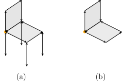
Figure 1. (a) An arbitrary (non-reduced, length-16) loop on a rectangular lattice is shown. The ‘chair legs’ are edges present in the combination $e\bar{e}$. (b) Its reduced version. Notice that both paths have the same holonomy, though the path in (a) is larger than (b) in eight (the four removed combinations $e_{i}\bar{e}_{i}$ at the legs).

$$\gamma=e_{\circ}^{\epsilon_{1}}\alpha_{1}e_{\circ}^{\epsilon_{2}}\alpha_{2}\cdots e_{\circ}^{\epsilon_{m}}\alpha_{m}=:\textstyle\prod_{i=1}^{m}e_{\circ}^{\epsilon_{i}}\alpha_{i}$$ (3.1a)

(cf. Fig. 2) where each of $$\epsilon_{1},\epsilon_{2},\ldots,\epsilon_{m}\in\{+1,-1\} e_{\circ}^{\epsilon}={{\bar{e}_{\circ}}} {e_{\circ}} \epsilon=-1 e_{\circ}^{\epsilon} {e_{\circ}} \epsilon=1 \gamma {e_{\circ}} \epsilon_{1}=1 \alpha_{1},\ldots,\alpha_{m}\subset\gamma {e_{\circ}} {{\bar{e}_{\circ}}} \alpha_{j} \beta {e_{\circ}} {e_{\circ}} {{\bar{e}_{\circ}}} \beta$$ is a sign. This convention means that is the edge backwards if , while of course is itself if . (The condition that starts with implies above, but leaving this implicit is convenient.) By asking that each subpath does not contain neither nor , one uniquely determines the ’s. For another loop , which also starts with , under the same assumption that and do not appear consecutively in in any order, a similar decomposition holds

$$\beta =e_{\circ}^{\sigma_{1}}\mu_{1}e_{\circ}^{\sigma_{2}}\mu_{2}\cdots e_{\circ}^{\sigma_{p}}\mu_{p}$$ (3.1b)

in terms of signs $\sigma_{j}\in\{-1,+1\}$ and paths $\mu_{j}$ not containing neither the rooted edge ${e_{\circ}}$ nor ${{\bar{e}_{\circ}}}$. The only difference in notation —which we will keep throughout— is that $\gamma$ will refer to generalised plaquettes (i.e. contribution to the spectral action) while $\beta$ will be the path of a Wilson loop.

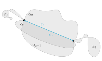
Figure 2. The most general reduced path $\gamma=e_{\circ}^{\epsilon_{1}}\alpha_{1}e_{\circ}^{\epsilon_{2}}\alpha_{2}\cdots e_{\circ}^{\epsilon_{m}}\alpha_{m}$ containing $e_{\circ}$ and/or ${{\bar{e}_{\circ}}}$ is shown here (omitting orientations for sake of simplicity). The most general Wilson loop can also be decomposed in subpaths in a similar way, cf. eqs. (3.1).

Take again the polynomial $f(x)=f_{0}+f_{1}x+f_{2}x^{2}+\ldots+f_{d}x^{d}$, and rephrase the spectral action of eq. (2.3) as

$$S(D_{Q})=\operatorname{Tr}f(D_{Q})=\sum_{\begin{subarray}{c}\gamma\in\Omega Q\\ \gamma\text{ reduced }\end{subarray}}g_{\gamma}\operatorname{Tr}\operatorname{\mathrm{hol}}\gamma.\qquad$$ (3.2)

Now $g_{\gamma}$ is a function of $f_{\ell(\gamma)}$ but possibly also of $f_{\ell(\gamma)+2},f_{\ell(\gamma)+4},\ldots$, whenever these last coefficients are non-zero. The contribution of the higher coefficients is owed to the appearance in larger paths of a contiguous pair of edges $e,\bar{e}$ for which the respective unitarities will satisfy $U_{e}U^{*}_{e}=1=U_{e}^{*}U_{e}$. These cancellations are not detected by the holonomy, which is the criterion used in (3.2) to collect all terms (instead of using, as in eq. (2.3), the $f_{0},\ldots,f_{d}$ coefficients and performing directly the sum over paths). For instance, if $\gamma$ is the path in Fig. 1 (b), then $g_{\gamma}$ depends on $f_{\ell(\gamma)}$ and $f_{\ell(\gamma)+8}$, since Fig. 1 (a) contributes the same to the spectral action. The function $g_{\gamma}=g_{\gamma}(f_{0},f_{1},\ldots,f_{d})$ is of course quiver-dependent.

3.2. Main statement

The Makeenko-Migdal or loop equations we are about to generalise appeared first in lattice quantum chromodynamics [MM79]. They have been a fundamental ingredient in the construction of Yang-Mills theory in [Lév17, DGHK17, CPS23] in rigorous probabilistic terms.

Theorem 3.1 (Makeenko-Migdal equations for the spectral action on quivers).

Let $R$ be a representation of a connected quiver $Q$ and let $N=\dim R$. Root an edge ${e_{\circ}}$ of $Q$ that is not a self-loop and abbreviate by $U=U_{{e_{\circ}}}$ the unitarity that $R$ determines for ${e_{\circ}}$. Then for any reduced loop $\beta$, decomposed as $\beta=e_{\circ}^{\sigma_{1}}\mu_{1}e_{\circ}^{\sigma_{2}}\mu_{2}\cdots e_{\circ}^{\sigma_{p}}\mu_{p}$ according to eq. (3.1b), the following relation among Wilson loops holds:

$$\mathbb{E}\bigg{[}\sum_{\begin{subarray}{c}j=1\\ \sigma_{j}=+1\end{subarray}}^{p}\frac{1}{N}\operatorname{Tr}(U^{\sigma_{1}}\operatorname{\mathrm{hol}}\mu_{1}\cdots U^{\sigma_{j-1}}\operatorname{\mathrm{hol}}\mu_{j-1})\frac{1}{N}\operatorname{Tr}(U^{\sigma_{j}}\operatorname{\mathrm{hol}}\mu_{j}\cdots U^{\sigma_{p}}\operatorname{\mathrm{hol}}\mu_{p})$$

$$\,\,-\sum_{\begin{subarray}{c}j=1\\ \sigma_{j}=-1\end{subarray}}^{p}\frac{1}{N}\operatorname{Tr}(\operatorname{\mathrm{hol}}\mu_{1}U^{\sigma_{2}}\operatorname{\mathrm{hol}}\mu_{2}\cdots U^{\sigma_{j-1}}\operatorname{\mathrm{hol}}\mu_{j-1})\frac{1}{N}\operatorname{Tr}(\operatorname{\mathrm{hol}}\mu_{j}U^{\sigma_{j+1}}\cdots U^{\sigma_{p}}\operatorname{\mathrm{hol}}\mu_{p})\bigg{]}$$

$$=\sum_{\begin{subarray}{c}\gamma\in S(D)\\ \gamma\text{ \scriptsize reduced }\\ \gamma=\prod_{i=1}^{m(\gamma)}e_{\circ}^{\epsilon_{i}}\alpha_{i}\end{subarray}}g_{\gamma}\mathbb{E}\bigg{[}\sum_{\begin{subarray}{c}j=1\\ \epsilon_{j}=+1\end{subarray}}^{m(\gamma)}\frac{1}{N}\operatorname{Tr}(\operatorname{\mathrm{hol}}\beta\cdot U^{\epsilon_{j}}\operatorname{\mathrm{hol}}\alpha_{j}\cdots\operatorname{\mathrm{hol}}\alpha_{m}U^{\epsilon_{1}}\operatorname{\mathrm{hol}}\alpha_{1}\cdots U^{\epsilon_{j-1}}\operatorname{\mathrm{hol}}\alpha_{j-1})$$ (3.3)

$$\qquad\qquad\qquad\qquad\!-\sum_{\begin{subarray}{c}j=1\\ \epsilon_{j}=-1\end{subarray}}^{m(\gamma)}\frac{1}{N}\operatorname{Tr}(\operatorname{\mathrm{hol}}\beta\cdot\operatorname{\mathrm{hol}}\alpha_{j}U^{\epsilon_{j+1}}\cdots\operatorname{\mathrm{hol}}\alpha_{m}U^{\epsilon_{1}}\operatorname{\mathrm{hol}}\alpha_{1}\cdots\operatorname{\mathrm{hol}}\alpha_{j-1}U^{\epsilon_{j}})\bigg{]},$$

where the dependence $\gamma=e_{\circ}^{\epsilon_{1}(\gamma)}\alpha_{1}e_{\circ}^{\epsilon_{2}(\gamma)}\alpha_{2}\cdots e_{\circ}^{\epsilon_{m(\gamma)}}\alpha_{m(\gamma)}$ on the signs $\epsilon_{i}$ and the subpaths $\alpha_{i}$ on $\gamma$ is left implicit for sake of notation.

Remark 3.2.

Some special cases of eqs. (3.3) are commented on:

1. The second line (lhs) takes the expectation value of $\tfrac{1}{N}\operatorname{Tr}(U^{\sigma_{1}}\operatorname{\mathrm{hol}}\mu_{1}\cdots U^{\sigma_{j-1}}\operatorname{\mathrm{hol}}\mu_{j-1}U^{\sigma_{j}})$ $\times\frac{1}{N}\operatorname{Tr}(\operatorname{\mathrm{hol}}\mu_{j}\cdots U^{\sigma_{p}}\operatorname{\mathrm{hol}}\mu_{p})$, but $\sigma_{j}$ being $-1$ allows for a cancellation, hence the apparent lack of harmony between the first two lines of the lhs.

2. We also stress that the first term in the lhs, which corresponds to $j=1=\sigma_{1}$, yields the input Wilson loop $\beta$ in the first trace and a constant path in the second; the latter yields a factor of $N$, which is cancelled by its prefactor.

3. If neither ${{\bar{e}_{\circ}}}$ nor ${e_{\circ}}$ are along $\gamma$, then $m(\gamma)=0$ and the respective sum is empty (the rhs is zero).

4. Similarly, if neither ${{\bar{e}_{\circ}}}$ nor ${e_{\circ}}$ are on $\beta$, which is the case of the constant loop, $p=0$ and the sum in question is empty (the lhs is zero).

5. Suppose that the plaquettes in the action $S(D)=\sum_{\gamma}^{\text{\tiny reduced}}\tilde{g}_{\gamma}[\operatorname{Tr}\operatorname{\mathrm{hol}}\gamma+\operatorname{Tr}\operatorname{\mathrm{hol}}\bar{\gamma}]$, intersect each either ${e_{\circ}}$ or ${{\bar{e}_{\circ}}}$ exactly once. Notice that this time we have rewritten it as sum over pairs $\gamma$ and $\bar{\gamma}$ (which is always possible since the paths are in $\Gamma Q$ and the spectral action is real valued). Then

   $$\mathbb{E}\bigg{[}\sum_{\begin{subarray}{c}j=1\\ \sigma_{j}=+1\end{subarray}}^{p}\frac{1}{N}\operatorname{Tr}(U\operatorname{\mathrm{hol}}\mu_{1}\cdots U^{\sigma_{j-1}}\operatorname{\mathrm{hol}}\mu_{j-1})\frac{1}{N}\operatorname{Tr}(U^{\sigma_{j}}\operatorname{\mathrm{hol}}\mu_{j}\cdots U^{\sigma_{p}}\operatorname{\mathrm{hol}}\mu_{p})$$

   $$\,\,-\sum_{\begin{subarray}{c}j=1\\ \sigma_{j}=-1\end{subarray}}^{p}\frac{1}{N}\operatorname{Tr}(\operatorname{\mathrm{hol}}\mu_{1}\cdots U^{\sigma_{j-1}}\operatorname{\mathrm{hol}}\mu_{j-1})\frac{1}{N}\operatorname{Tr}(\operatorname{\mathrm{hol}}\mu_{j}\cdots U^{\sigma_{p}}\operatorname{\mathrm{hol}}\mu_{p})\,\bigg{]}$$

   $$=\sum_{\begin{subarray}{c}\gamma\in S(D)\\ \gamma=(U,\alpha)\text{ \scriptsize reduced }\end{subarray}}\tilde{g}_{\gamma}\mathbb{E}\bigg{[}\frac{1}{N}\operatorname{Tr}(\operatorname{\mathrm{hol}}\beta\cdot U\operatorname{\mathrm{hol}}\alpha)-\frac{1}{N}\operatorname{Tr}(\operatorname{\mathrm{hol}}\beta\operatorname{\mathrm{hol}}\bar{\alpha}\cdot U^{*})\bigg{]}.$$ (3.4)

Proof.

Consider the unitarity $U_{e_{\circ}}$ associated to the rooted edge ${e_{\circ}}\in Q_{1}$, and consider as given by a fixed ${\mathscr{pS}}$-representation $R=\{(A_{v},H_{v}),(\phi_{e},U_{e})\}_{v,e}$ of $Q$. Next, consider the infinitesimal variation of the spectral action by the change of variable exclusively for the unitarity $U_{e_{\circ}}$ at the edge ${e_{\circ}}$ as follows. Let

$$U_{e_{\circ}}\mapsto U_{e_{\circ}}^{\prime}=\mathrm{e}^{\imath Y}U_{e_{\circ}},\qquad\imath Y\in\mathfrak{su}(N),\qquad\imath=\sqrt{-1},$$ (3.5)

where $Y$ is given in terms of arbitrary matrices $\imath y_{k}\in\mathfrak{su}(n_{t(e),k})$ for $k=1,2,\ldots,l_{t({e_{\circ}})}=:L$ by

$$\mathrm{e}^{\imath Y}:=\operatorname{\mathrm{diag}}\big{[}1_{r_{t(e),1}}\otimes\exp({\imath y_{1}}),1_{r_{t(e),2}}\otimes\exp({\imath y_{2}}),\ldots,1_{r_{t(e),{L}}}\otimes\exp(\imath y_{L})\big{]}.$$

(Recall Sec. 2.3 for notation). One should keep in mind that this implies also the substitution $U_{e_{\circ}}^{*}\mapsto(U_{e_{\circ}}^{\prime})^{*}=U_{e_{\circ}}^{*}\mathrm{e}^{-\imath Y}$, as it follows from the change (3.5). This rule defines a new representation $R^{\prime}$ differing from $R$ only by the value of the unitarities at the edge ${e_{\circ}}$, that is

$$R^{\prime}=\{(A_{v},H_{v}),(\phi_{e},\exp(\delta_{e,{e_{\circ}}}\imath Y)U_{e}\}_{v\in Q_{0},e\in Q_{1}},$$ (3.6)

where $\delta_{e,e^{\prime}}$ is the indicator function on the edge-set.

The loop or Dyson-Schwinger or (in the unitary case) Makeenko-Migdal equations follow from

$$\int\sum_{a,b=1}^{N}(\partial_{Y})_{a,b}\{(\operatorname{\mathrm{hol}}_{R^{\prime}}\beta)_{b,a}\times\mathrm{e}^{-NS(D^{\prime})}\}{\mathrm{d}}D=0,\qquad D^{\prime}=D_{Q}{(R^{\prime})}.$$ (3.7)

(The entries of the matrix derivative are $(\partial_{Y})_{a,b}=\partial/\partial Y_{b,a}$ when $Y$ is hermitian.) This follows from the invariance of the Haar measure at the rooted edge under the transformation (3.5), yielding ${\mathrm{d}}D^{\prime}={\mathrm{d}}D$. Below, we show that this implies

$$\mathbb{E}\bigg{[}\Big{(}\frac{1}{N}\operatorname{Tr}\otimes\frac{1}{N}\operatorname{Tr}\Big{)}(\partial_{Y}\operatorname{\mathrm{hol}}\beta)\bigg{]}=\mathbb{E}\bigg{[}\frac{1}{N}\operatorname{Tr}(\partial_{Y}S\operatorname{\mathrm{hol}}\beta)\bigg{]},$$ (3.8)

and compute each quantity inside the trace(s). On the lhs, the matrix derivative acts on a noncommutative polynomial and is then the Rota-Stein-Turnbull noncommutative derivation

$$\partial_{Y}Y^{k+1}=\sum_{l=0}^{k}Y^{l}\otimes Y^{k-l}\qquad(Y^{*}=Y\in M_{N}(\mathbb{C}),k\in\mathbb{Z}_{\geq 0})$$ (3.9)

while on the rhs, the matrix yields Voiculescu’s cyclic derivation $\mathcal{D}_{Y}$, since the quantity it derives, $S$, contains a trace. Such derivative $\mathcal{D}_{Y_{j}}$ is defined, say for $q\in\mathbb{Z}_{>0}$, on the free algebra $\mathbb{C}_{\langle q\rangle}=\mathbb{C}\langle Y_{1},\ldots,Y_{q}\rangle$ on a monic noncommutative monomial $\psi$ by

$$\mathcal{D}_{Y_{j}}\psi(Y_{1},\ldots,Y_{q})=\sum_{\begin{subarray}{c}P,\Lambda\in\mathbb{C}_{\langle q\rangle}\\ \psi=\Lambda Y_{j}P\end{subarray}}P\Lambda.$$ (3.10)

(The sum is performed over all splittings by $Y_{j}$ of the word $\psi$ [Gui09, Sec. 7.2.2], wherein $P$ or $\Lambda$ might be empty).

Recalling that holonomies are multiplicative, one has $\operatorname{\mathrm{hol}}\gamma=U^{\epsilon_{1}}\operatorname{\mathrm{hol}}\alpha_{1}U^{\epsilon_{2}}\operatorname{\mathrm{hol}}\alpha_{2}U^{\epsilon_{3}}\cdots\operatorname{\mathrm{hol}}\alpha_{m-1}$ $U^{\epsilon_{m}}\operatorname{\mathrm{hol}}\alpha_{m}$. With respect to the transformed representation $R^{\prime}$ we can compute the holonomy $\operatorname{\mathrm{hol}}_{R^{\prime}}\delta$ of any path $\delta$. This depends on $Y$ and ${e_{\circ}}$ but we use a prime in favor of a light notation and write $\operatorname{\mathrm{hol}}^{\prime}\delta$. Since none of the subpaths $\alpha_{j}$ contains the transformed edges ${e_{\circ}}$ and ${{\bar{e}_{\circ}}}$, one has $\operatorname{\mathrm{hol}}^{\prime}\alpha_{j}=\operatorname{\mathrm{hol}}\alpha_{j}$, so

$$\operatorname{\mathrm{hol}}^{\prime}(\gamma)=U^{{}^{\prime}\epsilon_{1}}\operatorname{\mathrm{hol}}\alpha_{1}U^{{}^{\prime}\epsilon_{2}}\operatorname{\mathrm{hol}}\alpha_{2}U^{{}^{\prime}\epsilon_{3}}\cdots U^{{}^{\prime}\epsilon_{m}}\operatorname{\mathrm{hol}}\alpha_{m}$$ (3.11)

where $U^{{}^{\prime}\epsilon}$ is $\mathrm{e}^{\imath Y}U$ if $\epsilon=1$ and $U^{*}\mathrm{e}^{-\imath Y}$ if $\epsilon=-1$. Therefore the variation of the loop $\gamma$ writes

$$[\partial_{Y}\operatorname{Tr}\operatorname{\mathrm{hol}}^{\prime}\gamma]\big{|}_{Y=0} =\imath\sum_{\begin{subarray}{c}j=1\\ \epsilon_{j}=+1\end{subarray}}^{m}U\operatorname{\mathrm{hol}}\alpha_{j}U^{\epsilon_{j+1}}\operatorname{\mathrm{hol}}\alpha_{j+1}\cdots U^{\epsilon_{n}}\operatorname{\mathrm{hol}}\alpha_{n}U^{\epsilon_{1}}\operatorname{\mathrm{hol}}\alpha_{1}\cdots U^{\epsilon_{j-1}}\operatorname{\mathrm{hol}}\alpha_{j-1}$$

$$-\imath\sum_{\begin{subarray}{c}j=1\\ \epsilon_{j}=-1\end{subarray}}^{m}\operatorname{\mathrm{hol}}\alpha_{j}U^{\epsilon_{j+1}}\operatorname{\mathrm{hol}}\alpha_{j+1}\cdots U^{\epsilon_{n}}\operatorname{\mathrm{hol}}\alpha_{n}U^{\epsilon_{1}}\operatorname{\mathrm{hol}}\alpha_{1}\cdots U^{\epsilon_{j-1}}\operatorname{\mathrm{hol}}\alpha_{j-1}U^{*}.$$

The cyclic wandering of any fix holonomy, say $\operatorname{\mathrm{hol}}\alpha_{1}$, in the rhs of the main result is due to Voiculescu’s cyclic derivation (3.10).

We now compute the variation of the Wilson line $\beta$, whose holonomy writes for the representation $R^{\prime}$ as $\operatorname{\mathrm{hol}}^{\prime}\beta=\prod_{j=1}^{p}(U^{\prime})^{\sigma_{j}}\operatorname{\mathrm{hol}}^{\prime}\mu_{j}=\prod_{j=1}^{p}(U^{\prime})^{\sigma_{j}}\operatorname{\mathrm{hol}}\mu_{j}$. To take the variation observe that $\operatorname{\mathrm{hol}}^{\prime}\beta$ is not inside a trace. For any $A,B\in M_{N}(\mathbb{C})$, and $a,b,c,d=1,\ldots,N$, due to eq. (3.9),

$$(\partial_{Y})_{a,b}[A\exp(\imath Y)B]_{c,d}\bigg{|}_{Y=0} =\sum_{k=0}^{\infty}\frac{\imath^{k}}{k!}\sum_{l=0}^{k}A_{c,r}[Y^{l}\otimes Y^{k-1-l}]_{r,a|b,s}\bigg{|}_{Y=0}B_{s,d}=\imath A_{c,r}\delta_{r,a}\delta_{b,s}B_{s,d}.$$

Using this rule for the previous expression of $\operatorname{\mathrm{hol}}^{\prime}\beta$, one obtains a summand for each occurrence of $U^{\pm 1}$ and the result follows after equating the indices $c=a$, and $b=d$, which is the initial situation in the initial identity (3.7). ∎

3.3. Graphical representation of the Makeenko-Migdal equations

We illustrate graphically the meaning of the Makeenko-Migdal equations. Let us place ${e_{\circ}}$ and the reversed edge ${{\bar{e}_{\circ}}}$ along a fixed axis of the picture. To represent a Wilson loop $\beta$ or a reduced generalised plaquette $\gamma$, we choose the following notation. In order to avoid drawings with several intersections, for each time that $\gamma$ or $\beta$ walks along either ${e_{\circ}}$ or ${{\bar{e}_{\circ}}}$, we jump to the next ‘plane’ in anti-clockwise direction around the fixed axis. Thus each of these planes represents abstractly the subpath $\mu_{j}\subset\beta$ or $\alpha_{j}\subset\gamma$ according to the decompositions (3.1a) and (3.1b), that is:

We kept a rectangular appearance for sake of visual simplicity, but the subpaths $\mu_{j}$ and $\alpha_{j}$ are arbitrary (as far as they have positive length). In fact, the depicted situation is due to a second reason still oversimplified: the theorem describes the more general case that $\mu_{j}$ or $\alpha_{j}$ might be loops themselves (as $\alpha_{3}$ in Fig. 2), but this would render the pictures unreadable. The representation of the Makeenko-Migdal equations reads then as follows:

$$\text{ $\frac{1}{N^{2}}\times$}\bBigg@{18.30}(\raisebox{-0.5pt}{ \includegraphics[width=173.35933pt]{MM_LHS}}\bBigg@{18.30})\,\text{ $=\sum_{\gamma}g_{\gamma}$ }\bBigg@{14.030}(\!\!\!\raisebox{-0.5pt}{ \includegraphics[width=157.4069pt]{MM_RHS}}\bBigg@{14.030}$$

In the rhs, the very similar upper and lower terms need a word of notation. The blue arrow denotes an insertion of $U$ and is executed right after the green part of the path, while the red arrow inserts $U^{*}$ and follows only after the purple set of paths.

4. Applications

This last section aims at illustrating the power of the equations derived here when combined with the positivity conditions. This combination, sometimes known as ‘bootstrap’, appeared in [AK17] for lattice gauge theory and [Lin20] in a string context (for hermitian multimatrix models).

4.1. Positivity constraints

Let $v\in Q_{0}$ be fixed for this subsection and fix a representation $R$ of $Q$ of dimension $N$. Consider a complex variable $z_{\beta}$ for each loop $\beta$ based at a fixed vertex $v\in Q_{0}$, $z=\{z_{\beta}:\beta\in\Omega_{v}(Q)\}$, as well as the matrix

$$P(z):=\sum_{\begin{subarray}{c}\beta\in\Omega_{v}(Q)\end{subarray}}z_{\beta}\operatorname{\mathrm{hol}}\beta,\qquad P(z)\in M_{N}(\mathbb{C}).$$ (4.1)

It follows that $\operatorname{Tr}\big{[}P(z)P(z)^{*}\big{]}=\sum_{\beta,\alpha}z_{\beta}z^{*}_{\alpha}\operatorname{\mathrm{hol}}\beta\cdot(\operatorname{\mathrm{hol}}\alpha)^{*}=\sum_{\beta,\alpha\in\Omega_{v}(Q)}z_{\beta}z^{*}_{\alpha}\operatorname{\mathrm{hol}}(\beta\bar{\alpha})\geq 0$ independently of the $z$-tuple; this is preserved by expectation values, i.e.

$$\sum_{\beta,\alpha\in\Omega_{v}(Q)}z_{\beta}z^{*}_{\alpha}\mathbb{E}[\operatorname{\mathrm{hol}}(\beta\bar{\alpha})]\geq 0,\qquad\text{for all }z\in\mathbb{C}^{\Omega_{v}(Q)},$$ (4.2)

which is an equivalent way to state the positivity $\mathcal{M}\succeq 0$ of the matrix $\mathcal{M}\in\mathbb{C}[\![N,f_{0},f_{1},\ldots,f_{d}]\!]$ whose entries are given by

$$(\mathcal{M})_{i,j}:=\mathbb{E}[\operatorname{\mathrm{hol}}(\beta_{i}\bar{\beta}_{j})]$$ (4.3)

for any ordering of the loops $\{\beta_{1},\beta_{2},\ldots\}\subset\Omega_{v}(Q)$ at the fixed vertex $v$. The positivity of $\mathcal{M}$ is clearly independent of the way we order these loops, as a conjugation by a permutation matrix (which is a unitary transformation) will not change the eigenvalues of $\mathcal{M}$.

Figure 3. The matrix entries for a $2\times 2$ submatrix of $\mathcal{M}$ (before taking expectation values) are shown in this figure. On the diagonal the trivial entries one sees result from the (holonomy of both) loops cancelling, which has the holonomy of the constant path. On the off-diagonal entries, one sees a non-trivial loop composition that goes first around the orange arrows and then along the green ones.

The paths $\beta_{i}$ and $\beta_{j}$ feeding the matrix (4.3) need only to satisfy $s(\beta_{i})=s(\beta_{j})$ and $t(\beta_{j})=t(\beta_{i})$ so that $\beta_{i}\bar{\beta}_{j}$ is a loop; the assumption that $\beta_{i}$ and $\beta_{j}$ themselves are loops is not essential. The choice for the matrix (4.3) with loop entries is originally from [KZ24], who pushed forward the bootstrap for lattice Yang-Mills theory. The techniques of [Lin20] were implemented for fuzzy spectral triples for an interesting kind of hermitian matrix [HKP22] and a hermitian 2-matrix model [KP24]. The loop equations of [MM79] have been extended here to include arbitrary plaquettes that whirl around any edge more than once, and Wilson loops that are allowed to do the same.

4.2. A complete example

Consider the triangle quiver $Q=\raisebox{-3.48747pt}{\includegraphics[height=29.02193pt]{triangulo_blau}}$ with a rooted edge ${e_{\circ}}$, and let $\zeta={e_{\circ}}\mu$ be the only loop of length 3 starting with ${e_{\circ}}$ ($\mu$ is the path $v_{2}\to v_{3}\to v_{1}$, of course). Fix the the Bratteli network $B$ given by $A_{v_{i}}=M_{N}(\mathbb{C}),H_{v_{i}}=\mathbb{C}^{N}$ for the three vertices, $i=1,2,3$ (the transition matrices $C_{e}$ have all one entry equal to 1, for the three vertices). The space $\operatorname{\mathscr{D}}(B)$ of Dirac operators is therefore three copies of $\mathrm{U}(N)$, and the corresponding partition function

$$\mathcal{Z}_{Q,B}=\int_{\mathrm{U}(N)^{3}}\mathrm{e}^{-NS(D(U_{1},U_{2},U_{3}))}{\mathrm{d}}U_{1}{\mathrm{d}}U_{2}{\mathrm{d}}U_{3}.$$ (4.4)

The action $S(D)=\operatorname{Tr}f(D)$ for $f(t)=f_{0}+f_{1}t+f_{2}t^{2}+f_{3}t^{3}$ with real coefficients reads

$$S(D)=(f_{0}+2f_{2})N+x[\operatorname{Tr}\operatorname{\mathrm{hol}}\zeta+\operatorname{Tr}\operatorname{\mathrm{hol}}\zeta^{-1}],$$ (4.5)

where we set $x=3f_{3}$. The terms in the even coefficients are just constants that disappear when evaluating Wilson loops; we therefore set $f_{0}=f_{2}=0$.

4.2.1. Loop equations

Now pick a loop $\beta=\zeta^{n}$ for positive $n\in\mathbb{Z}$. According to the loop equations (3.4), one has

$$\mathbb{E}\bigg{[}\sum_{k=0}^{n-1}(\frac{1}{N}\operatorname{Tr}\otimes\frac{1}{N}\operatorname{Tr})(\operatorname{\mathrm{hol}}\zeta^{k}\otimes\operatorname{\mathrm{hol}}\zeta^{n-k})\bigg{]}=\frac{x}{N}(\mathbb{E}\operatorname{Tr}\operatorname{\mathrm{hol}}\zeta^{n+1}-\mathbb{E}\operatorname{Tr}\operatorname{\mathrm{hol}}\zeta^{n-1}).$$ (4.6)

Defining the large-$N$ moments by $m_{j}:=\lim_{N\to\infty}\mathbb{E}[\tfrac{1}{N}\operatorname{Tr}\operatorname{\mathrm{hol}}\zeta^{j}]$ for each $j\in\mathbb{Z}$, this means

$$\sum_{l=0}^{n-1}m_{l}\cdot m_{n-l}=x(m_{n+1}-m_{n-1}),\qquad(N\to\infty),$$ (4.7)

since large-$N$ factorisation holds, $N^{-2}\mathbb{E}[\operatorname{Tr}\operatorname{\mathrm{hol}}\zeta^{i}\operatorname{Tr}\operatorname{\mathrm{hol}}\zeta^{j}]\to m_{i}\cdot m_{j}$, as $N\to\infty$. For the loop $\beta=\zeta^{-n}$ with $n\in\mathbb{Z}_{>0}$, one has

$$-\sum_{j=0}^{n-1}m_{-(n-j)}\cdot m_{-j}=x(m_{-(n-1)}-m_{-(n+1)}),\qquad(N\to\infty).$$ (4.8)

Finally, going through the derivation of the loop equations for the constant Wilson loop, one obtains the vanishing of the lhs, so $0=x(m_{1}-m_{-1})$, hence $\bar{m}_{1}=\overline{\mathbb{E}[\operatorname{Tr}\operatorname{\mathrm{hol}}\zeta]}={\mathbb{E}[\operatorname{Tr}\operatorname{\mathrm{hol}}\bar{\zeta}]}={\mathbb{E}[\operatorname{Tr}\operatorname{\mathrm{hol}}\zeta^{-1}]}=m_{-1}=m_{1}$, so $m_{1}$ is real (this can be derived by other means, but the loop equations yield this explicitly). Together with eq. (4.8), this implies $m_{-j}=m_{j}$ for all $j=1,2,\ldots$ and the moments can be arranged in the following (due to $\mathcal{M}_{i,j}=\mathcal{M}_{i+k,j+k}$, Toeplitz-)matrix:

$$\mathcal{M}=\begin{bmatrix}1&m_{1}&m_{2}&m_{3}&\ldots&\\ m_{-1}&1&m_{1}&m_{2}&\ldots&\\ m_{-2}&m_{-1}&1&m_{1}&\ldots&\\ m_{-3}&m_{-2}&m_{-1}&1&\ldots&\\ \vdots&\vdots&\vdots&\vdots&\ddots\end{bmatrix}=\begin{bmatrix}1&m_{1}&m_{2}&m_{3}&\ldots&\\ m_{1}&1&m_{1}&m_{2}&\ldots&\\ m_{2}&m_{1}&1&m_{1}&\ldots&\\ m_{3}&m_{2}&m_{1}&1&\ldots&\\ \vdots&\vdots&\vdots&\vdots&\ddots\end{bmatrix}.$$ (4.9)

4.2.2. Bootstrap

Thanks to Theorem 3.1, $\mathcal{M}$ can be computed recursively in terms of $y:=m_{1}$ and the coupling $x$,

$$m_{1} =y m_{4} =\frac{4y}{x}+\frac{3y^{2}}{x^{2}}+\frac{1}{x^{2}}+\frac{y}{x^{3}}+1$$

$$m_{2} =\frac{y}{x}+1 m_{5} =y+\frac{3y^{2}}{x}+\frac{2y^{3}}{x^{2}}+\frac{3}{x}+\frac{9y}{x^{2}}+\frac{6y^{2}}{x^{3}}+\frac{1}{x^{3}}+\frac{y}{x^{4}}$$

$$m_{3} =y+\frac{y^{2}}{x}+\frac{1}{x}+\frac{y}{x^{2}} m_{6} =\frac{9y}{x}+\frac{18y^{2}}{x^{2}}+\frac{10y^{3}}{x^{3}}+\frac{6}{x^{2}}+\frac{16y}{x^{3}}+\frac{10y^{2}}{x^{4}}+\frac{1}{x^{4}}+\frac{y}{x^{5}}+1.$$

The positivity condition $\mathcal{M}(x,y)\succeq 0$ can be plotted on the first moment vs. coupling plane in terms of the simultaneous positivity of its minors $\mathcal{M}_{n}(x,y):=[\mathcal{M}(x,y)_{a,b}]_{a,b=1,\ldots,n}$. as done in Figure 4 for $n=1,\ldots,6$.

         

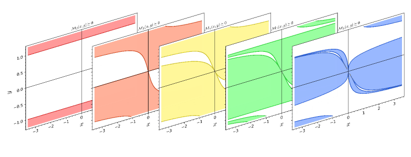
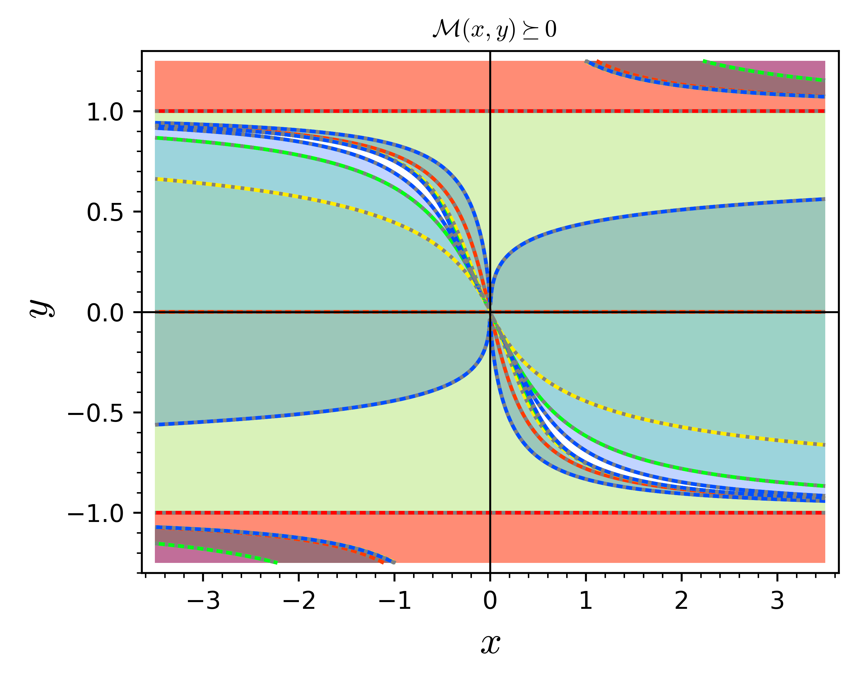
Figure 4. On the panel above, the colored regions violate $\mathcal{M}(x,y)\succeq 0$ as a consequence of the minors $\mathcal{M}_{n}(x,y)$ satisfying $\det\mathcal{M}_{n}(x,y)<0$ for $n=1$ (tautological, not drawn), $n=2$ (the complement to the stripe $|y|<1$), $n=3$ (orange), $n=4$ (yellow), $n=5$ (green) and $n=6$ (blue). Superposition of all these plots yields the plot below, in which only in the narrow white region satisfies the simultaneous conditions $\det\mathcal{M}_{n}(x,y)>0$, $n=1,2,\ldots,6$. Fig. 6 goes further, but due to readability shows only the seventh minor, which narrows down even more the white space. Script and plots use SageMath [S⁺09].

4.2.3. Exact solution

Let us contrast this strategy with the analytic solution. The partition function (4.4) can be simplified by integrating over a single unitary group, $U=U_{1}U_{2}U_{3}$,

$$\mathcal{Z}_{Q,B} =\int_{\mathrm{U}(N)^{3}}\mathrm{e}^{-Nx\operatorname{Tr}(U_{1}U_{2}U_{3}+U_{3}^{*}U_{2}^{*}U_{1}^{*})}{\mathrm{d}}U_{1}{\mathrm{d}}U_{2}{\mathrm{d}}U_{3}$$

$$=\Bigg{(}\int_{\mathrm{U}(N)}{\mathrm{d}}U_{1}\Bigg{)}\Bigg{(}\int_{\mathrm{U}(N)}{\mathrm{d}}U_{2}\Bigg{)}\int_{\mathrm{U}(N)}\mathrm{e}^{-Nx\operatorname{Tr}(U+U^{*})}{\mathrm{d}}U$$

$$=\int_{\mathrm{U}(N)}\mathrm{e}^{-Nx\operatorname{Tr}(U+U^{*})}{\mathrm{d}}U=:\mathcal{Z}_{N}(x).$$ (4.10)

We now contrast the positivity constraints with the exact solution by Wadia and Grosse-Witten (GWW). Their strategy was to diagonalise the integration variable as $U=V\Theta V^{*}$, by a $V\in\mathrm{U}(N)$, being $\Theta=\operatorname{\mathrm{diag}}(\mathrm{e}^{\imath\theta_{1}},\mathrm{e}^{\imath\theta_{2}},\ldots,\mathrm{e}^{\imath\theta_{N}})\in\mathrm{U}(1)^{N}$. This yields an integral over the torus $\mathrm{U}(1)^{N}$ of $\prod_{j=1}^{N}\mathrm{e}^{-2Nx\cos\theta_{j}}\times\prod_{1\leq i<k\leq N}|\mathrm{e}^{\imath\theta_{i}}-\mathrm{e}^{\imath\theta_{k}}|^{2}$. The last factor is of the form $\det(\Delta)\det(\Delta^{*})$, where $\Delta_{m,n}=\exp(n\imath\theta_{m})$ is the Vandermonde matrix from the change of variable. The explicit expression solution is [Wad79, GW80]

$$\mathcal{Z}_{N}(x) =\det[I_{k-m}(-2xN)]_{k,m=1,\ldots,N}:=\det\begin{pmatrix}I_{0}(z)&I_{1}(z)&\cdots&I_{N-1}(z)\\ I_{-1}(z)&I_{0}(z)&\cdots&I_{N-2}(z)\\ \vdots&\vdots&\ddots&\vdots\\ I_{-(N-1)}(z)&I_{-(N-2)}(z)&\cdots&I_{0}(z)\end{pmatrix}_{z=-2xN}$$

for the partition function as the determinant of a Toeplitz matrix of Bessel $I$-functions,

$$I_{q}(z):=\frac{1}{2\pi}\int_{0}^{2\pi}\mathrm{e}^{\imath q\alpha+z\cos\alpha}{\mathrm{d}}\alpha,$$ (4.11)

evaluated at $z=-2xN$. Armed with this explicit solution, the exact moment $y_{N}=\mathbb{E}[\frac{1}{N}\operatorname{Tr}\operatorname{\mathrm{hol}}\zeta]$ by eq. (4.10) reads (the expectation values of $\operatorname{Tr}\operatorname{\mathrm{hol}}\zeta$ and $\operatorname{Tr}\operatorname{\mathrm{hol}}\zeta^{-1}$ coincide, hence the factor $\tfrac{1}{2}$)

$$y_{N}(x)=-\frac{1}{2\mathcal{Z}_{N}(x)N^{2}}\frac{\partial}{\partial x}\mathcal{Z}_{N}(x).$$ (4.12)

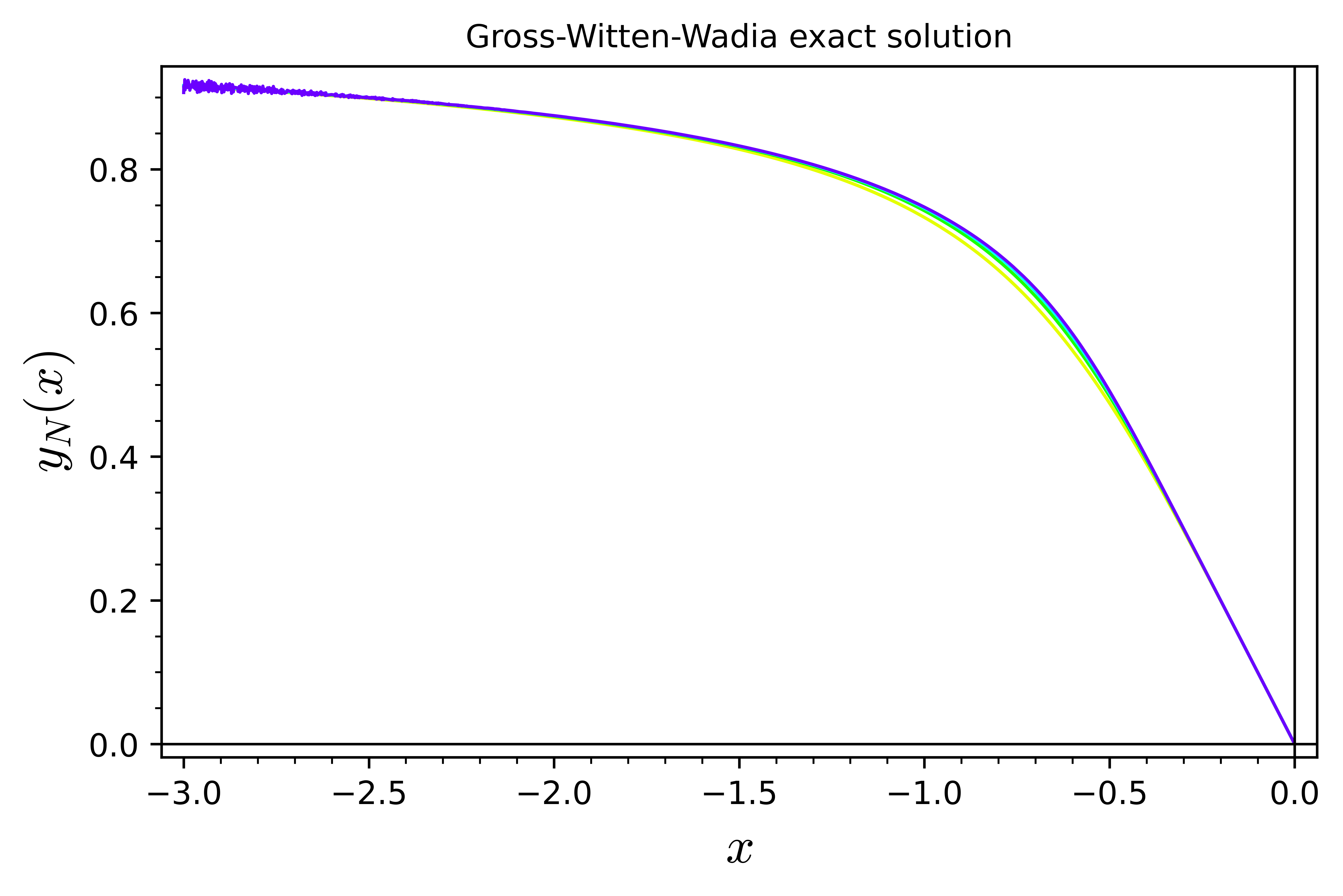
Figure 5. The expectation value of $\frac{1}{N}\operatorname{Tr}\operatorname{\mathrm{hol}}\zeta=\frac{1}{N}\operatorname{Tr}[U_{1}U_{2}U_{3}]$ computed from the exact partition function $\mathcal{Z}_{N}(x)$ via $y_{N}(x)=(-1/2\mathcal{Z}_{N}(x)N^{2})\partial_{x}\mathcal{Z}_{N}(x)$ at finite $N$, namely for $N\in\{\color[rgb]{0.78,1,0.13}2,\color[rgb]{0,1,0.4}3,\color[rgb]{0,1,1}4,\color[rgb]{0.25,0.1,1}5\color[rgb]{0,0,0}\}$. Cf. comparison with the bootstrap solution in Fig. 6.

This was plotted for different values of $N$ in Figure 5. If our loop equations are correct, then the curve $y_{N}(x)$ should lie inside the region where $\mathcal{M}(x,y)$ is non-negative for large enough $N$ (agreement only at large $N$ is expected since freeness or factorisation of the expectation values was used to compute the matrix of moments and $\mathcal{M}$). Luckily, this is what clearly happens in the plots of Figure 6: the highest technically feasible computation for $\mathcal{M}(x,y)$ yielded a very tight constraint where the expectation value $y_{N}$ computed from the GWW partition function embeds.

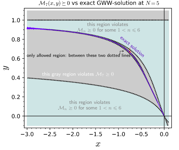
Figure 6. Comparison of the darker gray region that violates $\mathcal{M}_{7}(x,y)\succeq 0$ with the exact GWW-solution at $N=5$ in solid color line. The large light blue regions around the gray bulk are excluded by testing the minors $\mathcal{M}_{n}(x,y)$ for $n\leq 6$. This leaves only a narrow allowed region between the ‘parallel’ paths tagged with an arrow; there sits the exact solution, plotted here for $N=5$.

4.3. Concluding remarks and outlook

The results of this article can be summarised as follows. Given the two first elements of the spectral triple $A_{Q},H_{Q}$ associated to a quiver $Q$ (equivalent to a Bratteli network on $Q$), we characterised the ensemble of Dirac operators $D$ that complete $(A_{Q},H_{Q},D)$ into a spectral triple, as well as the mesure ${\mathrm{d}}D$ on such ensemble. The partition function

$$\mathcal{Z}_{A,H}(f)=\int_{\!\!\!\!\begin{subarray}{c}\phantom{nictu}\\[3.01389pt] (A,H,D)\text{ \scriptsize is}\\ \text{ \scriptsize spectral triple}\end{subarray}}\mathrm{e}^{-NS(D)}{\mathrm{d}}D,\quad S(D)=\operatorname{Tr}f(D),\quad N=\dim H.$$ (4.13)

is made concrete here. Since ${\mathrm{d}}D$ is a Haar measure, unitarity invariance leads to constraints for the Wilson loops of this theory. Such loop equations were proven and applied in combination with positivity conditions in the case of a simple example.

As happened above, the observed situation for a large class of hermitian matrix integrals are tight constraints for the first moment (or for a finite set of moments) in terms of the coupling, which, by increasing the size of the minors, typically determine a curve $y=y(x)$—and by the respective loop equations, all the moments and thus the solution of the model. In this article we do not claim the convergence of a ‘bootstrapped’ solution in all ensembles of unitary matrices. The aim of this example was to illustrate the usefulness of the loop equations proven here. But the results of this example do encourage us to explore this combination in future works, including also a hermitian (‘Higgs scalar’) field that arises from the self-loops of the quiver.

References

- [AK17] Peter D. Anderson and Martin Kruczenski. Loop Equations and bootstrap methods in the lattice. Nucl. Phys. B, 921:702–726, 2017.
- [AK24] Shahab Azarfar and Masoud Khalkhali. Random finite noncommutative geometries and topological recursion. Ann. Inst. Henri Poincaré D, Comb. Phys. Interact., 11(3):409–451, 2024.
- [Bar15] John W. Barrett. Matrix geometries and fuzzy spaces as finite spectral triples. J. Math. Phys., 56(8):082301, 2015.
- [BG16] John W. Barrett and Lisa Glaser. Monte Carlo simulations of random non-commutative geometries. J. Phys. A, 49(24):245001, 2016.
- [BHGW22] Johannes Branahl, Alexander Hock, Harald Grosse, and Raimar Wulkenhaar. From scalar fields on quantum spaces to blobbed topological recursion. J. Phys. A, Math. Theor., 55(42):30, 2022. Id/No 423001.
- [Bra72] Ola Bratteli. Inductive limits of finite dimensional C∗-algebras. Trans. Am. Math. Soc., 171:195–234, 1972.
- [CC97] Ali H. Chamseddine and Alain Connes. The Spectral action principle. Commun. Math. Phys., 186:731–750, 1997.
- [CC06] Alain Connes and Ali H. Chamseddine. Inner fluctuations of the spectral action. J. Geom. Phys., 57:1–21, 2006.
- [CGL24] Benoît Collins, Răzvan Gurău, and Luca Lionni. The tensor Harish-Chandra–Itzykson–Zuber integral I: Weingarten calculus and a generalization of monotone Hurwitz numbers. J. Eur. Math. Soc., 26(5):1851–1897, 2024.
- [CM08] Alain Connes and Matilde Marcolli. Noncommutative geometry, quantum fields and motives, volume 47 of Texts Read. Math. New Delhi: Hindustan Book Agency, 2008.
- [Col03] Benoît Collins. Moments and cumulants of polynomial random variables on unitarygroups, the Itzykson-Zuber integral, and free probability. Int. Math. Res. Not., 2003(17):953–982, 2003.
- [Conn94] Alain Connes. Noncommutative geometry. 1994.
- [Conn13] Alain Connes. On the spectral characterization of manifolds. J. Noncommut. Geom., 7:1–82, 2013.
- [CPS23] Sky Cao, Minjae Park, and Scott Sheffield. Random surfaces and lattice Yang-Mills. 7 2023. arXiv:2307.06790.
- [CŚ06] Benoît Collins and Piotr Śniady. Integration with Respect to the Haar Measure on Unitary, Orthogonal and Symplectic Group. Commun. Math. Phys., 264(3):773–795, 2006.
- [CvS21] Alain Connes and Walter D. van Suijlekom. Spectral truncations in noncommutative geometry and operator systems. Commun. Math. Phys., 383(3):2021–2067, 2021.
- [CvS22] Alain Connes and Walter D. van Suijlekom. Tolerance relations and operator systems. Acta Sci. Math., 88(1-2):101–129, 2022.
- [DGHK17] Bruce K. Driver, Franck Gabriel, Brian C. Hall, and Todd Kemp. The Makeenko-Migdal equation for Yang-Mills theory on compact surfaces. Commun. Math. Phys., 352(3):967–978, 2017.
- [DLL22] Francesco D’Andrea, Giovanni Landi, and Fedele Lizzi. Tolerance relations and quantization. Lett. Math. Phys., 112(4):28, 2022. Id/No 65.
- [DW17] Harm Derksen and Jerzy Weyman. An introduction to quiver representations, volume 184 of Grad. Stud. Math. Providence, RI: American Mathematical Society (AMS), 2017.
- [GHW20] Harald Grosse, Alexander Hock, and Raimar Wulkenhaar. Solution of the self-dual QFT-model on four-dimensional Moyal space. J. High Energy Phys., 2020(1):17, 2020. Id/No 81.
- [GNS22] James Gaunt, Hans Nguyen, and Alexander Schenkel. BV quantization of dynamical fuzzy spectral triples. J. Phys. A, 55(47):474004, 2022.
- [GW80] D. J. Gross and Edward Witten. Possible Third Order Phase Transition in the Large N Lattice Gauge Theory. Phys. Rev. D, 21:446–453, 1980.
- [GW14] Harald Grosse and Raimar Wulkenhaar. Self-dual noncommutative -theory in four dimensions is a non-perturbatively solvable and non-trivial quantum field theory. Commun. Math. Phys., 329(3):1069–1130, 2014.
- [Gui09] Alice Guionnet. Large random matrices: Lectures on macroscopic asymptotics. École d’Été des Probabilités de Saint-Flour XXXVI – 2006, volume 1957 of Lect. Notes Math. Berlin: Springer, 2009.
- [HKP22] Hamed Hessam, Masoud Khalkhali, and Nathan Pagliaroli. Bootstrapping Dirac ensembles. J. Phys. A, 55(33):335204, 2022.
- [HKPV22] Hamed Hessam, Masoud Khalkhali, Nathan Pagliaroli, and Luuk S. Verhoeven. From noncommutative geometry to random matrix theory. J. Phys. A, 55(41):413002, 2022.
- [IvS17] Roberta A. Iseppi and Walter D. van Suijlekom. Noncommutative geometry and the BV formalism: application to a matrix model. J. Geom. Phys., 120:129–141, 2017.
- [Kon92] Maxim Kontsevich. Intersection theory on the moduli space of curves and the matrix Airy function. Commun. Math. Phys., 147(1):1–23, 1992.
- [KP21] Masoud Khalkhali and Nathan Pagliaroli. Phase Transition in Random Noncommutative Geometries. J. Phys. A, 54(3):035202, 2021.
- [KP24] Masoud Khalkhali and Nathan Pagliaroli. Coloured combinatorial maps and quartic bi-tracial 2-matrix ensembles from noncommutative geometry. JHEP, 05:186, 2024.
- [KPV24] Masoud Khalkhali, Nathan Pagliaroli, and Luuk S. Verhoeven. Large N limit of fuzzy geometries coupled to fermions. 2024. arXiv:2405.05056.
- [Kra98] Thomas Krajewski. Classification of finite spectral triples. J. Geom. Phys., 28:1–30, 1998.
- [KZ24] Vladimir Kazakov and Zechuan Zheng. Bootstrap for Finite N Lattice Yang-Mills Theory. 4 2024. arXiv:2404.16925.
- [Lév17] Thierry Lévy. The master field on the plane, volume 388 of Astérisque. Paris: Société Mathématique de France (SMF), 2017.
- [Lin20] Henry W. Lin. Bootstraps to strings: solving random matrix models with positivity. JHEP, 06:090, 2020.
- [MM79] Yu. M. Makeenko and Alexander A. Migdal. Exact Equation for the Loop Average in Multicolor QCD. Phys. Lett. B, 88:135, 1979. [Erratum: Phys.Lett.B 89, 437 (1980)].
- [MN23] Thierry Masson and Gaston Nieuviarts. Lifting Bratteli diagrams between Krajewski diagrams: Spectral triples, spectral actions, and AF algebras. J. Geom. Phys., 187:104784, 2023.
- [MvS14] Matilde Marcolli and Walter D. van Suijlekom. Gauge networks in noncommutative geometry. J. Geom. Phys., 75:71–91, 2014.
- [NSS21] Hans Nguyen, Alexander Schenkel, and Richard J. Szabo. Batalin-Vilkovisky quantization of fuzzy field theories. Lett. Math. Phys., 111:149, 2021.
- [PS98] Mario Paschke and Andrzej Sitarz. Discrete sprectral triples and their symmetries. J. Math. Phys., 39:6191–6205, 1998.
- [Pér21] Carlos I. Pérez-Sánchez. On Multimatrix Models Motivated by Random Noncommutative Geometry I: The Functional Renormalization Group as a Flow in the Free Algebra. Annales Henri Poincare, 22(9):3095–3148, 2021.
- [Pér22a] Carlos I. Pérez-Sánchez. Computing the spectral action for fuzzy geometries: from random noncommutative geometry to bi-tracial multimatrix models. J. Noncommut. Geom., 16(4):1137–1178, 2022.
- [Pér22b] Carlos I. Pérez-Sánchez. On Multimatrix Models Motivated by Random Noncommutative Geometry II: A Yang-Mills-Higgs Matrix Model. Annales Henri Poincare, 23(6):1979–2023, 2022.
- [Pér24] Carlos I. Pérez-Sánchez. The Spectral Action on quivers. 2024. arXiv:2401.03705.
- [Rie10] Marc A. Rieffel. Leibniz seminorms for “Matrix algebras converge to the sphere”. Clay Math. Proc., 11:543–578, 2010.
- [Rie23] Marc A. Rieffel. Dirac Operators for Matrix Algebras Converging to Coadjoint Orbits. Commun. Math. Phys., 401(2):1951–2009, 2023.
- [S+09] SageMath, the Sage Mathematics Software System (Version 9.5), The Sage Developers, 2024, https://www.sagemath.org.
- [StSz08] Harold Steinacker and Richard J. Szabo. Localization for Yang-Mills theory on the fuzzy sphere. Commun. Math. Phys., 278:193–252, 2008.
- [vNvS21] Teun D. H. van Nuland and Walter D. van Suijlekom. Cyclic cocycles in the spectral action. J. Noncommut. Geom., 16(3):1103–1135, 2021.
- [vS11] Walter D. van Suijlekom. Perturbations and operator trace functions. J. Funct. Anal., 260(8):2483–2496, 2011.
- [vS15] Walter D. van Suijlekom. Noncommutative geometry and particle physics. Mathematical Physics Studies. Springer, Dordrecht, 2015.
- [Wad79] Spenta Wadia. A study of U lattice gauge theory in two-dimensions. 1979. arXiv:1212.2906 (TeX’ed from the ‘79 original).