Fair Minimum Representation Clustering via Integer Programming

Abstract

Clustering is an unsupervised learning task that aims to partition data into a set of clusters. In many applications, these clusters correspond to real-world constructs (e.g., electoral districts, playlists, TV channels) whose benefit can only be attained by groups when they reach a minimum level of representation (e.g., 50% to elect their desired candidate). In this paper, we study the k-means and k-medians clustering problems with the additional constraint that each group (e.g., demographic group) must have a minimum level of representation in at least a given number of clusters. We formulate the problem through a mixed-integer optimization framework and present an alternating minimization algorithm, called MiniReL, that directly incorporates the fairness constraints. While incorporating the fairness criteria leads to an NP-Hard assignment problem within the algorithm, we provide computational approaches that make the algorithm practical even for large datasets. Numerical results show that the approach is able to create fairer clusters with practically no increase in the clustering cost across standard benchmark datasets.

1 Introduction

Clustering is an unsupervised learning task that aims to partition data points into sets of similar data points called clusters (Xu and Wunsch,, 2005). Clustering is widely used due to its broad applicability in domains such as customer segmentation (Kansal et al.,, 2018), grouping content together for entertainment platforms (Daudpota et al.,, 2019), and identifying subgroups within a clinical study (Wang et al.,, 2020) amongst others. However the wide-spread application of clustering, and machine learning broadly, to human-centric applications has raised concerns about its disparate impact on minority groups and other vulnerable demographics. Motivated by a flurry of recent results highlighting bias in many automated decision making tasks such as facial recognition (Buolamwini and Gebru,, 2018) and criminal justice (Mehrabi et al.,, 2019), researchers have begun focusing on mechanisms to ensure machine learning algorithms are fair to all those affected. One of the challenges of fairness in an unsupervised learning context, compared to the supervised setting, is the lack of ground truth labels. Consequently, instead of enforcing approximately equal error rates across groups, fair clustering generally aims to ensure that composition of the clusters or their centers (for settings like $k$-means and $k$-medians clustering) represent all groups fairly.

A common approach to fair clustering is to require each cluster to have a fair proportion of itself represented by each group (i.e., via balance (Chierichetti et al.,, 2017) or bounded representation (Ahmadian et al.,, 2019)). This approach aims to balance the presence of each group in each cluster and therefore tries to spread each group uniformly across the clusters. Notice that this approach might not be desirable in settings where a group only gains a significant benefit from the cluster when they reach a minimum level of representation in that cluster. Consider the problem of clustering a set of media (e.g., songs, tv shows) into cohesive segments (e.g., playlists, channels). A natural fairness consideration in designing these segments would be to ensure that there is sufficient representation for different demographic groups. In these settings the benefit of the representation is only realized when a large percentage of the segment is associated with a demographic group (i.e., so that listeners can consistently watch or hear programming that speaks to them). This is even legislated in some countries, for example Canadian television channels are required to have at least 50% Canadian programming (Brownwell,, 2015). Note that, in this setting, spreading a minority demographic group across all clusters ensures that the demographic group will never have majority representation in any segment.

As another example, consider a simple voting system for a committee where the goal is to first cluster voters (e.g., employees, faculty) into different constituencies that can then elect a committee representative. Here, a proportionally fair clustering would assign a minority group that represents 30% of the vote equally among each cluster. However, the minority group only gets a benefit (i.e., the ability to elect a candidate of their choice) if they have at least 50% representation in the cluster. In this paper we introduce a new notion of fairness in clustering that addresses this issue. Specifically, we introduce minimum representation fairness (MR-fairness) which requires each group to have a certain number of clusters where they cross a given minimum representation threshold (i.e., 50% in the voting example).

Arguably the most popular algorithms for clustering is Lloyd’s algorithm for $k$-means clustering (Jain et al.,, 1999), and the associated alternating minimization approach for $k$-medians (Park and Jun,, 2009). These iterative algorithms alternate between fixing cluster centers and assigning each point to the closest cluster center. Both algorithms are guaranteed to return a locally optimal solution (i.e., no perturbation of the cluster centers around the solution leads to a better clustering cost). However, using these algorithms can lead to clusters that violate MR-fairness. As an example, consider the Adult dataset which contains census data for 48842 individuals in 1994 (Dua et al.,, 2017). Suppose we wanted to cluster these individuals into groups that represent different stakeholder groups for a local committee and geographic contiguity was not a concern. A natural fairness criteria in this setting would be to ensure that there are a sufficient number of groups where minority groups (i.e., non-white in this dataset) have majority voting power. Despite the fact that only approximately 85% of the dataset is white, every cluster produced by Lloyd’s algorithm is dominated by white members even when the number of clusters is as high as twenty. This highlights the need for a new approach to address fair minority representation.

In this paper we introduce a modified version of Lloyd’s algorithm for $k$-means and $k$-medians that ensures minimum representation fairness, henceforth referred to as MINIimum REpresentation fair Lloyd’s algorithm (MiniReL for short). The key modification behind our approach is to replace the original greedy assignment step with a new optimization problem that finds the minimum cost assignment while ensuring fairness. In contrast to the standard clustering setting, we show that finding a minimum cost clustering that respects MR-fairness is NP-Hard even when the cluster centers are already fixed. We show that this optimization problem can be solved via integer programming (IP) in practice and introduce a number of computational approaches to improve the run-time. We empirically show that our approach is able to construct fair clusters which have nearly the same clustering cost as those produced by Lloyd’s algorithm.

1.1 Minimum Representation Fair Clustering Problem

The input to the standard clustering problem is a set of $n$ $m$-dimensional data points $\mathcal{X}=\{x^{i}\in\mathbbm{R}^{m}\}_{i=1}^{n}$. Note that assuming the data points to have real-valued features is not a restrictive assumption as categorical features can be converted to real-valued features through the one-hot encoding scheme. The goal of the clustering problem is to partition the data points into a set of $K$ clusters $\mathcal{C}=\{C_{1},\dots,C_{K}\}$ in such a way that some measure of clustering cost is minimized. Let ${\cal K}=\{1,\dots,K\}$ be the set of clusters.

In the fair clustering setting, each data point $x^{i}$ has a (small) number of sensitive features such as gender and race associated with it. Each sensitive feature can take a finite number of possible values (e.g., male, female, or non-binary for gender). We denote the set of sensitive features with ${\cal F}$ and possible values of a feature $f\in{\cal F}$ with the set ${\cal G}_{f}$. We use ${\cal G}=\cup_{f\in{\cal F}}{\cal G}_{f}$ to be the set of all possible values of all features, and call each $g\in{\cal G}$ a group. With this notation, each data point $x^{i}$ is associated with $|{\cal F}|$ many groups, one for each $f\in\mathcal{F}$ (i.e., gender, race). Let $X_{g}$ be the set of data points associated with group $g\in\mathcal{G}$ and note that unlike other fair machine learning work, we do not assume that $\{X_{g}\}_{g\in{\cal G}}$ form a partition of $\mathcal{X}$ when $|{\cal F}|>1$. Instead, $\{X_{g}\}_{g\in{\cal G}_{f}}$ forms a partition of $\mathcal{X}$ for each sensitive feature $f\in{\cal F}$.

The key intuition behind MR-fair clustering is that individuals belonging to a group gain material benefit only when they have a minimum level of representation in their cluster. We denote this minimum representation threshold $\alpha\in(0,1]$, and define the associated notion of an $\alpha$-representation as follows:

Definition 1 ($\alpha$-representation).

A group $g\in\mathcal{G}$ is said to be $\alpha$-represented in a cluster $C_{k}$ if

$$|C_{k}\cap X_{g}|\geq\alpha|C_{k}|$$

Note that $\alpha$ represents the minimum threshold needed for a given group to receive benefit from a cluster and thus depends on the application. For instance, most voting systems require majority representation (i.e., $\alpha=0.5$). Our framework also allows for $\alpha$ to be group-dependent (i.e., $\alpha_{g}$ for each group $g$), however in most applications of interest $\alpha$ is a fixed threshold regardless of group. For a given clustering $\mathcal{C}$, group $g\in{\cal G}$, and $\alpha\in(0,1]$, let $\Lambda(\mathcal{C},X_{g},\alpha)$ be the number of clusters where group $g$ has $\alpha$-represention. In MR-fairness, each group $g$ has a parameter $\beta_{g}$ that specifies a minimum number of clusters where that group should have $\alpha$-represention.

Definition 2 (Minimum representation fairness).

A given clustering $\mathcal{C}=\{C_{1},\dots,C_{K}\}$ is said to be an ($\alpha,\boldsymbol{\beta}$)-minimum representation fair clustering if for every group $g\in{\mathcal{G}}$:

$$\Lambda(\mathcal{C},X_{g},\alpha)\geq\beta_{g}$$

for a given $\boldsymbol{\beta}=\{\beta_{g}\in\mathbb{Z}^{+}\}_{g\in\mathcal{G}}$.

The definition of MR-fairness is flexible enough that the choice of $\boldsymbol{\beta}$ can (and should) be specialized to each application as well as the choice of $\alpha$. Also note that up to $\lfloor 1/\alpha\rfloor$ groups corresponding to a single feature $f$ can be $\alpha$-represented in a cluster. In the remainder of the paper we explore two different natural choices for $\boldsymbol{\beta}$ that mirror fairness definitions in the fair classification literature. The first sets $\beta_{g}$ to be equal for all groups corresponding to the same feature:

$$\beta_{g}=\Big{\lfloor}\frac{1}{|\mathcal{G}_{f}|}\big{\lfloor}\alpha^{-1}\big{\rfloor}K\Big{\rfloor}\quad\forall g\in\mathcal{G},f\in{\cal F}$$

which we denote cluster statistical parity. The second set choice sets $\beta_{g}$ to be proportional to the size of the group:

$$\beta_{g}=\Big{\lfloor}\frac{|X_{g}|}{n}\big{\lfloor}\alpha^{-1}\big{\rfloor}K\Big{\rfloor}\quad\forall g\in\mathcal{G}$$

which we denote cluster equality of opportunity. Note that in both cases, $\beta_{g}$ should be at most $K$ (i.e., if $\alpha$ is very small, we set $\beta_{g}=K$).

We integrate MR-fairness into two popular clustering paradigms: $k$-means and $k$-medians. In both settings the aim is to find a clustering together with a set of cluster centers $\{c_{k}\in{\cal L}_{k}\}_{k=1}^{K}$. In the $k$-means setting the center of a cluster can be located anywhere in the feature space (i.e., ${\cal L}_{k}=\mathbbm{R}^{m}~{}~{}\forall k$), whereas in $k$-medians it must be at one of the data points assigned to the cluster (i.e., ${\cal L}_{k}=C_{k}$). Note that in the standard $k$-medians setting it is not necessary to explicitly require $c_{k}\in C_{k}$ as any (local) optimal solution would satisfy this. However, this is no longer true in the MR-fairness setting and thus we explicitly constraint the center to belong to the cluster. We denote the cost of assigning a data point $x^{i}$ to a cluster with center $c$ with $D(x^{i},c)$ and the objective of the problem is to minimize the total cost of the clustering over all data points. In the $k$-means setting the cost is equal to the squared distance between the data point and the center (i.e., $D(x^{i},c)=\|x^{i}-c\|^{2}$), whereas in $k$-medians one can use any distance function. Combining the standard clustering problem with MR-fairness requirement leads to the following optimization problem:

Definition 3 (Minimum representation fair $k$-means and $k$-medians problem).

For a given $\alpha\in(0,1]$ and $\boldsymbol{\beta}=\{\beta_{g}\in\mathbb{Z}^{+}\}_{g\in\mathcal{G}}$, the minimum representation fair $k$-means and $k$-medians problems are:

$$\min_{\mathcal{C},c_{1},\ldots,c_{K}}\sum_{k\in\mathcal{K}}\sum_{x^{i}\in C_{k}}D(x^{i},c_{k})\quad\textbf{s.t.}\quad\Lambda(\mathcal{C},X_{g},\alpha)\geq\beta_{g}~{}~{}\forall g\in\mathcal{G},c_{k}\in{\cal L}_{k}~{}~{}\forall k\in{\cal K}$$

where ${\cal L}_{k}=\mathbbm{R}^{m}~{}~{}\forall k$, $D(x^{i},c)=\|x^{i}-c\|_{2}^{2}$  for $k$-means, and ${\cal L}_{k}=C_{k}$, $D(x^{i},c)$ is any given distance function for $k$-medians problem.

The main difference between the fair and the standard versions of the $k$-means and $k$-medians clustering problem is that greedily assigning data points to their closest cluster center may no longer be feasible for the fair version (i.e., assigning some data points to farther cluster centers may be necessary to meet the fairness criteria). Thus the problem can no longer be viewed as an optimization problem over cluster centers.

1.2 Related Work

A recent flurry of work in fair clustering has given rise to a number of different notions of fairness. One broad line of research, started by the seminal work of Chierichetti et al., (2017), puts constraints on the proportion of each cluster that comes from different groups. This can be in the form of balance (Chierichetti et al.,, 2017; Bera et al.,, 2019; Schmidt et al.,, 2018; Bercea et al.,, 2018; Backurs et al.,, 2019; Kleindessner et al., 2019b, ; Ahmadian et al.,, 2020; Böhm et al.,, 2020; Chhabra et al.,, 2020; Liu and Vicente,, 2021; Ziko et al.,, 2021; Le Quy et al.,, 2021) which ensures each group has relatively equal representation, or a group specific proportion such as the bounded representation criteria (Ahmadian et al.,, 2019; Bera et al.,, 2019; Ahmadian et al.,, 2020; Schmidt et al.,, 2018; Esmaeili et al.,, 2020; Jia et al.,, 2020; Huang et al.,, 2019; Bandyapadhyay et al.,, 2020; Harb and Lam,, 2020) or maximum fairness cost (Chhabra et al.,, 2020). MR-fairness bares a resemblance to this line of work as it puts a constraint on the proportion of a group in a cluster, however instead of constraining a fixed proportion across all clusters it looks holistically across all clusters and ensures that threshold is met in a baseline number of clusters. Another line of work tries to minimize the worst case average clustering cost (i.e., $k$-means cost) over all the groups, called social fairness (Ghadiri et al.,, 2021; Abbasi et al.,, 2021; Makarychev and Vakilian,, 2021; Goyal and Jaiswal,, 2021). Most similar to our algorithmic approach is the Fair Lloyd algorithm introduced in (Ghadiri et al.,, 2021) which studies social fairness. They also present a modified version of Lloyd’s algorithm that converges to a local optimum. As a consequence of the social fairness criterion their approach requires a modified center computation step that can be done in polynomial time. MR-fairness, however, requires a modified cluster assignment step that is NP-hard which we solve via integer programming.

Most similar to MR-fairness is diversity-aware fairness introduced in (Thejaswi et al.,, 2021) and the related notion of fair summarization (Kleindessner et al., 2019a, ; Chiplunkar et al.,, 2020; Jones et al.,, 2020). These notions of fairness require that amongst all the cluster centers selected, a minimum number comes from each group. MR-fairness differs in that our criteria is not tied to the group membership of the cluster center selected but the proportion of each group in a given cluster. Our notion of fairness is more relevant in settings where the center cannot be prescribed directly, but is only a function of its composition (i.e., in voting where members of a ‘cluster’ elect an official).

There is also a long line of research that looks at fairness in the context of gerrymandering (Kueng et al.,, 2019; Gurnee and Shmoys,, 2021; Benade et al.,, 2022; Levin and Friedler,, 2019; Mehrotra et al.,, 1998; Ricca et al.,, 2013). While our notion of fairness shares some similarity with different notions of fairness in gerrymandering, the gerrymandering problem places different constraints on the construction of the clusters such as contiguity. Consequently the algorithmic approaches to tackle gerrymandering generally require more computationally intensive optimization procedures that do not readily transfer to the machine learning setting.

1.3 Main Contributions

We summarize our main contributions as follows:

• We introduce a novel definition of fairness for clustering of practical importance called MR-fairness, which requires that a specified number of clusters should have at least $\alpha$ percent members from a given group.

• We formulate the problem of finding a MR-fair $k$-means or $k$-medians clustering in a mixed integer optimization framework, and introduce a new heuristic algorithm MiniReL, based on Lloyd’s algorithm for clustering, to find a local optimum.

• We show that unlike other notions of proportional fairness, this problem can not be approximated by adjusting unfair cluster centers.

• We show that incorporating MR-fairness into Lloyd’s algorithm leads to a NP-Hard sub-problem to assign data points to fixed cluster centers, which we call the Fair Minimum Representation Assignment (FMRA) Problem.

• We introduce a two-stage decomposition approach to solving the FMRA problem that includes a polynomial time bi-criteria approximation algorithm based on a network flow formulation. We also introduce a polynomial time heuristic for setting the first-stage variables.

• We present numerical results to demonstrate that MiniReL is able to construct MR-fair clusterings with only a modest increase in run-time and with little to no increase in clustering cost compared to the standard $k$-means or $k$ -medians clustering algorithm.

An initial version of this paper was published in a conference publication (Lawless and Günlük,, 2024) which introduced MR-fairness and a basic version of the MiniReL algorithm with pre-fixing. In this work we extend MiniReL to the $k$-medians setting and present new computational studies to show its efficacy. In addition, we build upon MiniReL’s algorithmic framework and introduce a two-stage decomposition framework to solve the FMRA including a polynomial time heuristic for solving the FMRA under pre-fixing built around a network flow model. We also provide additional theoretic results on the total unimodularity of the heuristic pre-fixing IP presented in the conference version, and additional NP-hardness results on variants of the FMRA problem.

The remainder of the paper is organized as follows. In Section 2 we present a mixed integer optimization formulation for the MR-fair clustering problem and introduce MiniReL. In Section 3 we introduce computational approaches to help our algorithm scale to large datasets. Finally Section 4 presents a numerical study of MiniReL compared to the standard Lloyd’s algorithm.

2 Mixed Integer Optimization Framework

We start by formulating the MR-fair $k$-means clustering problem as a mixed-integer program with a non-linear objective. We use binary variable $z_{ik}$ to denote if data point $x^{i}$ is assigned to cluster $k$, and variable $c_{k}\in\mathbb{R}^{d}$ to denote the center of cluster $k$. The binary variable $y_{gk}$ indicates whether group $g$ is $\alpha$-represented in cluster $k$. Let ${\cal L}_{k}(\textbf{z})$ be the set of allowable cluster center locations for cluster $k$ as a function of the current cluster assignments, (i.e., ${\cal L}_{k}(\mathbf{z})=\mathbbm{R}^{m}$ for $k$-means). To represent ${\cal L}_{k}$ in the $k$-medians case, we introduce additional binary decision variables $d_{ik}$ to denote if data point $i$ is selected as the center for cluster $k$. The set ${\cal L}_{k}(\mathbf{z})$ is the set defined by the following constraints:

$${\cal L}_{k}(\mathbf{z})~{}=~{}\mathopen{}\mathclose{{}\left\{c_{k}\in{\mathcal{R}}^{m}\;:\>c_{k}=\sum_{x^{i}\in{\cal X}}d_{ik}x^{i},\quad d_{ik}\leq z_{ik}~{}~{}\forall x^{i}\in{\cal X},\quad\sum_{x^{i}\in{\cal X}}d_{ik}=1,\quad d_{ik}\in\{0,1\}~{}~{}\forall x^{i}\in{\cal X}}\right\}$$

We can now formulate the MR-fair clustering problem as follows:

min $$\sum_{x^{i}\in{\mathcal{X}}}\sum_{k\in\mathcal{K}}D(x^{i},c_{k})z_{ik}$$ (1)

s.t. $$\sum_{k\in\mathcal{K}}z_{ik} =1~{}~{} \forall x^{i}\in{\mathcal{X}}$$ (2)

$$\sum_{x^{i}\in X_{g}}z_{ik}+M(1-y_{gk}) \geq\alpha\sum_{x^{i}\in{\mathcal{X}}}z_{ik}~{}~{} \forall g\in{\mathcal{G}},k\in{\mathcal{K}}$$ (3)

$$\sum_{k\in\mathcal{K}}y_{gk} \geq\beta_{g} \forall g\in{\mathcal{G}}$$ (4)

$$u\geq\sum_{x^{i}\in{\mathcal{X}}}z_{ik} \geq l \forall k\in{\mathcal{K}}$$ (5)

$$z_{ik} \in\{0,1\} \forall x^{i}\in\mathcal{X},k\in{\mathcal{K}}$$ (6)

$$y_{gk} \in\{0,1\} \forall g\in{\mathcal{G}},k\in{\mathcal{K}}$$ (7)

$$c_{k} \in{\cal L}_{k}(z) \forall k\in\mathcal{K}$$ (8)

The objective (1) is to minimize the cost of the clustering. Constraint (2) ensures that each data point is assigned to exactly one cluster. Constraint (3) tracks whether a cluster $k$ is $\alpha$-represented by a group $g$, and includes a big-$M$ which can be set to $\alpha n$. Finally, constraint (4) tracks that each group $g$ is $\alpha$-represented in at least $\beta_{g}$ clusters. In many applications of interest, it might also be worthwhile to add a constraint on the size of the clusters to ensure that each cluster has a minimum/maximum number of data points. Constraint (5) captures this notion of a cardinality constraint where $l$ and $u$ represent the lower and upper bound for the cardinality of each cluster respectively. Note that in cases where the cardinality constraint is used, the big-$M$ in constraint (3) can be reduced to $\alpha u$. In all our experiments we make sure that $l\geq 1$ so that exactly $k$ clusters are returned by the algorithm. This ensures that each group is $\alpha$-represented in non-trivial clusters. Note that every group would be trivially $\alpha$-represented in an empty cluster according to Definition 1 but would provide little practical use.

To solve problem (1)-(8) in practice, we introduce a modified version of Lloyd’s algorithm called MiniReL, which requires solving a fair assignment problem, in Section 2.1. In Section 2.2 we show that, unlike other notions of fairness in clustering, first solving the clustering problem without fairness constraints and then finding a fair assignment of the data points to these centers can lead to arbitrarily poor results under MR-fairness which further justifies the use of an iterative approach such as MiniReL.

2.1 MiniReL Algorithm for Fair Clustering

Solving the optimization problem outlined in the preceding section to optimality is computationally challenging as it is a large scale integer optimization problem with a non-convex objective function. To solve the problem in practice, we introduce a modified version of Lloyd’s algorithm which we call the Minimum Representation Fair Lloyd’s Algorithm (MiniReL) that alternates between adjusting cluster centers and fairly assigning data points to clusters to converge to a local optimum, see Algorithm 1.

Algorithm 1 (Minimum Representation Fair Lloyd’s Algorithm (MiniReL)
).

Input: Data $\mathcal{X}$, Number of clusters $K$, Fairness parameters $\boldsymbol{\beta}$, $\alpha$

Output: Cluster assignments $\{C_{k}\}_{k\in\mathcal{K}}$ and cluster centers $\{c_{k}\}_{k\in\mathcal{K}}$

1:  Initialize $\{c_{k}\}_{k\in\mathcal{K}}$ (for example by uniformly at random sampling $K$ data points).

2:  repeat

3:     Solve fair assignment problem (1)-(6) for fixed cluster centers $\{c_{k}\}_{k\in\mathcal{K}}$ to get optimal $\mathbf{z}$

4:     Compute the cost of solution current_cost

5:     for $k=1,2,\dots,K$ do

6:        if $k$-means then

7:           Set $N_{k}=\sum_{x^{i}\in\mathcal{X}}z_{ik}$, $c_{k}=\frac{1}{N_{k}}\sum_{x^{i}\in\mathcal{X}}z_{ik}x^{i}$.

8:        else if $k$-medians then

9:           Set $c_{k}=\operatorname{\arg\min}_{c\in{\cal X}}\sum_{x^{i}\in C_{k}}D(x^{i},c)$

10:        end if

11:     end for

12:     Compute the cost of solution improved_cost

13:  until improved_cost=current_cost

14:  Set $C_{k}=\{x^{i}\in\mathcal{X}:z_{ik}=1\}\quad\forall k\in\mathcal{K}$

15:  return $\{C_{k}\}_{k=1}^{K}$ and $\{c_{k}\}_{k\in\mathcal{K}}$

Note that the only difference between Lloyd’s algorithm for $k$-means and $k$-medians is how centers are computed. Given a fixed set of cluster assignments (i.e., when variables $z$ are fixed in (1)-(6)) the optimal choice of $c_{k}$ is the mean value of data points assigned to $C_{k}$ for $k$-means whereas it is found by searching across all data points in the cluster for $k$-medians (Park and Jun,, 2009). In the case of multiple centers with the same cost in the $k$-medians setting we use deterministic tie-breaking and chose the center corresponding to the data point that comes first in the lexicographic ordering of the dataset which we set-up at the beginning of the algorithm. For simplicity, we will refer to both algorithms (with separate center computation approaches) as Lloyd’s algorithm for the remainder of the paper. For a given (fixed) set of cluster centers $c_{k}$ we denote the problem (1)-(6) the fair minimum representation assignment (FMRA) problem which is a linear integer program. While the optimal assignment step in Lloyd’s algorithm can be done in polynomial time, the following result shows that the FMRA problem is NP-Hard.

Theorem 1.

The fair minimum representation assignment problem is NP-Hard.

See Appendix A for proof. Note that if the FMRA problem is infeasible (for any given collection of cluster centers), it provides a certificate that no MR-fair clustering with the given $\alpha$, $\beta$ exists. While integer programs do not always scale well to large datasets, in our computational experiments we observed that FMRA can be solved to optimality in a reasonable amount of time even for datasets with tens of thousands of data points. In Section 3 we describe the computational techniques that help scale our algorithm.

A natural question is whether MiniReL converges to a locally optimal solution as Lloyd’s algorithm does. When discussing local optimality, it is important to formally define the local neighborhood of a solution. In the absence of fairness constraints, data points must be assigned to the closest centers to minimize cost. Consequently, a clustering is locally optimal if perturbing the centers does not improve the clustering cost. In our setting, we define a local change as any perturbation to a cluster center, or an individual change to cluster assignment (i.e., moving a data point from one cluster to another). With this notion of a local neighborhood, the following result shows that the MiniReL converges to a local optimum in finite time. Note that while MiniReL converges to a local optimum, the solution may be arbitrarily worse than the global optimum as is the case for Lloyd’s algorithm.

Theorem 2.

MiniReL converges to a local optimum in finite time.

For proof please see Appendix B.

2.2 A Natural Solution Approach and an Inapproximability Result

One natural approach (Bera et al.,, 2019; Esmaeili et al.,, 2021, 2022) used for other notions of fairness in clustering is to first obtain cluster centers by solving the clustering problem without fairness constraints and then find a fair assignment of the data points to these centers. This has been shown to provide an overall approximation guarantee for the full optimization problem in some settings even when the centers are only approximately optimal for the clustering problem without fairness constraints (Bera et al.,, 2019; Esmaeili et al.,, 2021, 2022). Unfortunately, we show that in our MR-fairness setting this approach, which we call one-shot fair adjustment, can lead to arbitrarily bad solutions. Let $z^{*},c^{*}$ be the optimal solution to the MR-fair clustering problem. Let $c^{*}_{UF}$ be the optimal centers for the clustering problem without fairness constraints and $z^{*}_{FA}$ be the optimal (fair) assignment of data points to centers $c^{*}_{UF}$. Note both $z^{*}$ and $z^{*}_{FA}$ are feasible fair assignments. Let $COST(z,c)=\sum_{x^{i}\in{\mathcal{X}}}\sum_{k\in\mathcal{K}}D(x^{i},c_{k})z_{ik}$ be the objective for the clustering problem.

Theorem 3.

There does not exist a constant $M>0$ such that:

$$COST(z^{*}_{FA},c^{*}_{UF})\leq M\cdot COST(z^{*},c^{*})$$

In other words, fairly assigning data points to (approximately) optimal unfair centers can lead to arbitrarily bad performance relative to the optimal solution of the MR-fair clustering problem.

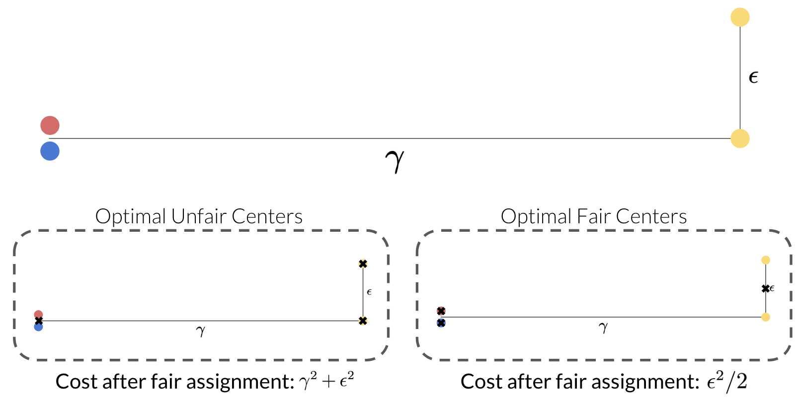
Figure 1: (Top) Bad instance of MR-fair clustering problem with four data points and three groups (represnted by colors). (Bottom Left) Optimal centers for the unfair clustering prioblem. (Bottom Right) Optimal centers for the MR-fair clustering problem.

Proof.

Proof of Theorem 3 To prove the claim we will construct an instance of the MR-fair $k$-means problem in two dimensions with four data points and three groups (Red, Blue, and Yellow). The first two points are located at $(0,0)$ and belong to the red and blue groups, respectively. The next two data points belong to the yellow group and are located at $(\gamma,0)$ and $(\gamma,\epsilon)$ for some $\gamma,\epsilon>0$. For the fair clustering problem, we set $K=3$, $\alpha>0.5$, and $\beta_{R}=\beta_{Y}=\beta_{B}=1$.

Note that any optimal solution to the clustering problem without fairness constraints will place the cluster centers $c^{*}_{UF}$ at $(0,0),(\gamma,0),(\gamma,\epsilon)$ with cost $0$. It is straightforward to see that fairly assigning points to these fixed centers requires assigning either the red or blue data point to the center at $(\gamma,0)$ and assigning the yellow data point at $(\gamma,0)$ to the center at $(\gamma,\epsilon)$ yielding a cost of $\gamma^{2}+\epsilon^{2}$. Now consider the optimal solution to the fair clustering problem which selects centers at $(0,0),(0,0),(\gamma,\epsilon/2)$. It assigns the red data point to the first center at $(0,0)$, the blue data point to the second center at $(0,0)$, and both yellow data points to the center at $(\gamma,\epsilon/2)$ which satisfies the fairness constraints and gives a total cost of $\epsilon^{2}/2$. The ratio of the costs of the two solutions is $\frac{\gamma^{2}+\epsilon^{2}}{\epsilon^{2}/2}$ which can be made arbitrarily large by increasing $\gamma$, completing the proof. Note that the same construction, with the same unfair centers and optimal fair centers at $(0,0),(0,0),(\gamma,0)$ proves the same result in the $k$-medians setting. Figure 1 shows both the bad instance and the optimal centers for the fair and unfair problems. ∎∎

Note that using the simple example constructed above, one can argue that the cost of the optimal fair clustering can be arbitrarily larger than the cost of the optimal clustering without fairness. Also note that the above proof also shows that one can get an arbitrarily bad solution when the (unfair) cluster centers are chosen using a constant factor approximation algorithm.

3 Scaling MiniReL: Two-Stage Decomposition

The main computational bottleneck of the MiniReL algorithm is solving the FMRA problem, which simultaneously selects which groups are $\alpha$-represented in which clusters (i.e., set $y_{gk}$ variables) and assigns data points to clusters in a way that satisfies said constraints (i.e. sets $z_{ik}$ variables). It is a computationally demanding problem to solve in practice both due to its scale (i.e., as the number of binary variables scales with the number of data points), symmetry, and its use of big-M constraints (i.e., that lead to weak linear relaxations (Conforti et al.,, 2014)). To alleviate these computational challenges, we introduce a heuristic two-stage decomposition scheme that separates setting the $y$ variables and $z$ variables into two sequential problems.

The first stage problem, which we call the Representation Assignment Problem  (RAP), sets the $y_{gk}$ variables. The second stage problem, which we call the Assignment Problem under Fixed Representation Constraints (APFRC), sets the $z_{ik}$ variables. One approach to solve the first-stage problem RAP is to solve the FMRA problem with relaxed $z$ variables (i.e., problem (1)-(8) with fixed centers, $y_{gk}$ binary and $z_{ik}\in[0,1]$). This dramatically reduces the number of binary variables (relaxing $nK$ binary variables), making the problem much faster to solve than FMRA in practice. While this approach does not guarantee the feasibility of an integral second-stage solution, in Section 3.2 we show that this fractional assignment can be rounded to an integer assignment with only small violation to the fairness constraints. In Section 3.1 we present an alternative heuristic approach to find a solution to the first-stage problem in polynomial time without the accompanying feasible fractional assignment of data points.

The second stage problem (APFRC) is akin to solving the FMRA problem with a fixed set of $y_{gk}$ variables. This removes the need for the $y$ variables and the associated big-M constraints in the model formulation and breaks symmetry in the IP (i.e., removes permutations of feasible cluster assignments), dramatically improving the computation time. However, despite this simplification, the following result shows that the second-stage problem is still NP-Hard.

Theorem 4.

The Assignment Problem under Fixed Representation Constraints Problem (APFRC) is NP-Hard.

See Appendix C for proof. Despite this negative result, in Section 3.2 we present a polynomial time algorithm that solves APFRC with a small additive fairness violation. We emphasize that this two-stage decomposition scheme is a heuristic which is not guaranteed to solve the FMRA problem to optimality. However, we found in practice this two-stage approach is able to find solutions that have similar objectives in a fraction of the time of solving the full IP (see Section 4.1 for an empirical evaluation). While both stages of the two-stage decomposition scheme can be solved sequentially at every iteration of the MiniReL algorithm, we found in practice the first stage solution changed infrequently during the execution of the algorithm. To further improve the computation time, we also present a pre-fixed version of the algorithm where we only set the $y_{gk}$ variables once at the beginning of the algorithm. In problems where only a single group can have $\alpha$-represention in a cluster (i.e., a data point can only be part of one group and $\alpha>0.5$), pre-fixing preserves an optimal solution to the full problem. However, in more complicated settings pre-fixing may remove all optimal solutions and becomes a heuristic for improving run-time. It is worth noting that the MiniReL algorithm is itself a heuristic, and thus the pre-fixing scheme has ambiguous effects on the cost of the solution as it may cause the algorithm to converge to a better local optimum. Figure 2 presents a visual summary of the three different control flows for the MiniReL algorithm.

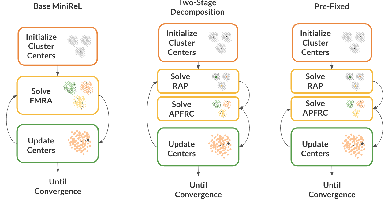
Figure 2: (Left) Base MiniReL algorithm where the assignment is doing by solving the full FMRA problem. (Center) MiniReL Algorithm with two-stage decomposition approach for solving the FMRA problem where we sequentially set $y_{gk}$ variables and $z_{ik}$ variables. (Right) Pre-fixed approach where the first stage problem to set $y_{gk}$ variables is only done once at beginning of algorithm.

3.1 Solving RAP via Polynomial Time Heuristic

Recall that the goal of the first stage problem is to find an assignment of groups to be $\alpha$-represented in clusters to meet the MR-fairness constraints. In this section we present a polynomial time heuristic to find good performing settings of the $y_{gk}$ variables.

To find a good pre-fixing of the $y$ variables, we use a fixed set of cluster centers and formulate a small integer program to find the lowest cost way to greedily meet the MR-fairenss constraints. There are multiple ways to formulate the cost of setting the $y$ variables - we look at the myopic increase in clustering cost needed to meet the constraints (see Appendix D for a computational comparison of different objectives). For a given cluster $k$ and group $g$, let $q_{kg}\geq 0$ be the additional number of points from group $g$ needed to make this group $\alpha$-represented in cluster $k$ (i.e., smallest integer $q_{kg}\geq 0$ that satisfies $q_{kg}+|C_{k}\cap X_{g}|\geq\alpha(q_{kg}+|C_{k}|)$). Let $c_{(x)}=\operatorname{\arg\min}_{c\in\{c_{1},\dots,c_{K}\}}\{\|x-c\|_{2}^{2}\}$ denote the closest center for point $x\in{\cal X}$. To find a good pre-fixing, we estimate the (myopic) increase in cost $m_{gk}$ to make group $g$ $\alpha$-represented in cluster $k$ as follows:

$$m_{gk}=\min_{X\subset X_{g}\setminus C_{K}:|X|=q_{kg}}\sum_{x\in X}\big{(}D(x^{i},c_{k})-D(x^{i},c_{(x)}))\big{)}$$

Note that this objective is a heuristic that does not take into account the impact of moving data points on the satisfaction of $\alpha$-representation constraints from the cluster in which it is being moved from. We can now formulate the problem of performing the pre-fix assignment as follows:

min $$\sum_{(g,k)\in{\mathcal{W}}}m_{gk}y_{gk}$$ (9)

s.t. $$\sum_{k\in\mathcal{K}:(g,k)\in\mathcal{W}}y_{gk} \geq\beta_{g}~{}~{} \forall g\in{\mathcal{G}}$$ (10)

$$\sum_{g\in\mathcal{G}_{f}}y_{gk} \leq\Big{\lfloor}\frac{1}{\alpha}\Big{\rfloor}~{}~{} \forall k\in\mathcal{K},f\in{\cal F}$$ (11)

$$y_{gk} \in\{0,1\}~{}~{} \forall g\in\mathcal{G},k\in\mathcal{K}$$ (12)

where $y_{g,k}$ is a binary variable indicating whether group $g$ will be $\alpha$-represented in cluster $k$. The objective (9) is a proxy for the cost of pre-fixing. Constraint (10) ensures enough clusters are allocated to each group to meet the MR-fairness constraint. Finally constraint (11) ensures no cluster is assigned more groups corresponding to the same feature than can simultaneously have $\alpha$-representation.

Note that the size of this formulation does not depend on the size of the dataset and it has only $|\mathcal{K}|\times|\mathcal{G}|$ variables. As mentioned earlier, when $\alpha>0.5$ and the groups are disjoint (i.e., no group can be in multiple groups) then this pre-fixing scheme simply removes symmetry. In other cases, this operation is a heuristic that leads to substantial speedups to the overall solution time. We now show that the constraint matrix for the pre-fixing problem (9)-(12) is totally unimodular, and thus can be solved in polynomial time.

Theorem 5.

The constraint matrix for the pre-fixing problem is totally unimodular.

Proof.

Proof of Theorem 5 Note that every variable $y_{gk}$ only appear in exactly two constraints - one constraint 10 for $g$ and one constraint 11 for $k$. Thus it suffices to show that there exists an equitable row bi-coloring for the full constraint matrix (Conforti et al.,, 2014). Set all constraints 10 to one color, and all constraints 11 to another color. Note that this is an equitable bi-coloring as the difference in row sums between the two colors will all be 0, completing the proof. ∎

3.2 Solving APFRC via Network Flow Rounding

In this section, we introduce a polynomial time algorithm to solve the second-stage APFRC problem while approximately meeting the fairness constraints. The key intuition behind our approach is that we take the fractional assignment of data points coming from the first stage RAP problem (or from solving the linear relaxation of the second stage problem) and round it to an integer assignment using a min-cost network flow model. Recall that in the APFRC problem, clusters have already been assigned groups that must be $\alpha$-represented in them (i.e., the $y_{gk}$ variables are fixed).

Given a fractional solution $\mbox{\boldmath$z$}^{LP}$, we construct a graph $G=(V,E)$ as follows. $V$ consists of three sets of vertices $V_{x}$, $V_{HK}$, $V_{K}$ which we define below. For every data point $x^{i}\in{\cal X}$ we construct a vertex $v_{i}\in V_{X}$ with a supply of 1. For every cluster $k$ we create a set of vertices $V_{HK}$ that partition the dataset (i.e., every data point can be mapped to exactly one vertex) and allow us to track how many data points of each group with $y_{gk}=1$ are assigned to cluster $k$. Let ${\cal G}_{k}$ be the set of groups $g$ such that $y_{gk}=1$. We create one vertex for every possible combination of attributes in the dataset such that the attribute corresponds to a group $g\in{\cal G}_{k}$ plus one ‘remainder’ vertex that corresponds to any other data point. For instance, consider a dataset with two sensitive features : Gender (Male, Female, Non-binary) and Age (Youth, Adult, Senior), and a cluster $k$ that was pre-fixed to have the Female, Youth, and Adult groups $\alpha$-represented. A set of combinations for the cluster are (Female, Youth), (Female, Adult), (Female, NOT {Youth or Adult}), (NOT Female, Youth), (NOT Female, Adult), and (NOT Female, NOT {Youth or Adult}). Let $H_{k}$ be the set of such combinations for a cluster $k$. For each combination of groups $c\in H_{k}$ we create create one node $v_{ck}\in V_{HK}$ with demand $d_{ck}=\lfloor\sum_{x^{i}\in\bigcap_{g\in c}X_{g}}z_{ik}^{LP}\rfloor$. We create an edge with capacity one between data point $x^{i}$ and every node $v_{ck}$ if $x^{i}\in\cap_{g\in c}X_{g}$. The cost for these edges is equal to the clustering cost of assigning $x^{i}$ to the fixed center $c_{k}$ (i.e., $D(x^{i},c_{k})$). The costs of all other edges in this graph are 0.

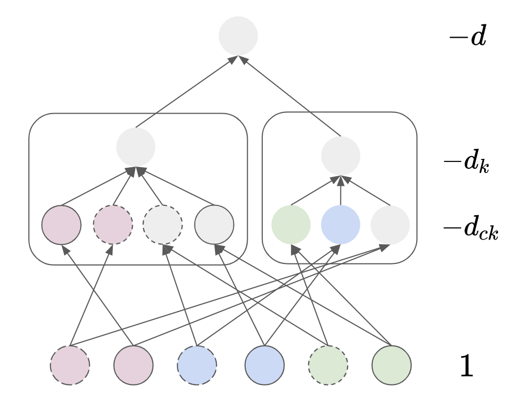
Figure 3: Sample network flow formulation for rounding the FMRA problem under pre-fixing with six data points, two clusters, and two sensitive attributes: Color (Purple, Blue or Green) and Border Type (Dashed or Solid). After pre-fixing, cluster 1 has to $\alpha$-represent both the Red and Dashed groups, and cluster 2 has to represent the green and blue groups. Vertex supplies (positive) and demand (negative) are indicated on the right hand side.

For every cluster $k$ we also create a node $v_{k}\in V_{K}$ with demand $d_{k}=\lfloor\sum_{x^{i}\in{\cal X}}z_{ik}^{LP}\rfloor-\sum_{c\in H_{k}}d_{ck}$. We create an edge with capacity one between every node $v_{k}$ and every node $v_{ck}$ corresponding to the same cluster. Finally, we add a sink note $v_{t}$ with demand $d=|{\cal X}|-\sum_{k}(d_{k}+\sum_{c\in H_{k}}d_{ck})$ to capture any residual supply. For every node $v_{k}\in V_{k}$ with fractional weight assigned to it in the LP solution (i.e., $\sum_{x^{i}\in{\cal X}}z^{LP}_{ik}\notin\mathbb{Z}$) we create an edge with capacity one between it and the node $v_{t}$. Figure 3 shows a sample network flow formulation. Note that this min-cost flow problem can be solved in polynomial time via standard min-cost flow algorithms (Williamson,, 2019). We denote the minimum cost flow problem associated with this graph the Flow-APFRC problem. We now show that by solving the Flow-APFRC problem we can generate a good assignment of data points to clusters:

Theorem 6.

Solving the Flow-APFRC problem yields a binary assignment of data points to clusters that respects the cardinality constraints and has a cost that does not exceed the cost of the LP relaxation of the APFRC problem.

Proof.

Proof Recall $\mbox{\boldmath$z$}^{LP}$ is the optimal fractional assignment of the APFRC problem (found by solving the LP relaxation or as the output of the RAP problem). We now construct an integer solution $\bar{\mbox{\boldmath$z$}}$ via solving the Flow-APFRC problem. Note that since all capacities and demands in the Flow-APFRC problem are integer, the optimal solution to the FMRA-problem is an integer flow. We can interpret this flow as a binary assignment of data points to clusters by setting $\bar{z}_{ik}=1$ if there is a unit of flow between vertex $v_{i}\in V_{\cal X}$ and any vertex $v\in V_{Hk}$, and 0 otherwise. By construction of the Flow-APFRC problem and the integrality of the optimal flow, we know every data point will be assigned to exactly one cluster. Since the LP solution is feasible for the network flow problem, we know that the cost of the solution $\bar{\textbf{z}}$ is lower or equal to the cost of the LP solution.

Note that at least $\lfloor\sum_{x^{i}\in{\cal X}}z_{ik}\rfloor$ and at most $\lceil\sum_{x^{i}\in{\cal X}}z_{ik}\rceil$ data points are assigned to cluster $k$. This follows from the fact that a total of $d_{k}+\sum_{c\in H_{k}}d_{ck}=\lfloor\sum_{x^{i}\in{\cal X}}z_{ik}\rfloor$ demand is consumed in nodes corresponding to cluster $k$ and the edge capacity of the edge of 1 between $v_{k}$ and $v_{t}$ ensures at most one additional point is allotted to cluster $k$. We now claim that the solution to the FMRA-flow problem satisfies the cardinality constraints. Suppose it did not, then $\lfloor\sum_{x^{i}\in{\cal X}}z_{ik}\rfloor<l$ or $\lceil\sum_{x^{i}\in{\cal X}}z_{ik}\rceil>u$. This implies that $\sum_{x^{i}\in{\cal X}}z_{ik}<l$ or $\sum_{x^{i}\in{\cal X}}z_{ik}>u$, which would violate constraints (5) and contradicts $\mbox{\boldmath$z$}^{LP}$ being a solution to the LP relaxation of the FMRA problem. ∎

It remains to show the impact of this rounding scheme on the fairness of the final solution. Specifically, we look at the impact of this network flow rounding procedure on the satisfaction of the $\alpha$-representation fairness constraints (i.e., constraints (3) for group $g$ and cluster $k$ where $y_{gk}=1$). Recall the following definition for an additive constraint violation:

Definition 4 (Additive Constraint Violation).

For a given constraint $g(x)\leq 0$, a solution $\bar{x}$ is said to have an additive constraint violation of $\delta$ for $\delta\geq 0$ such that $g(\bar{x})\leq\delta$.

We now show that the assignment produced by the Flow-APFRC problem has a small additive violation of the MR-fairness constraints.

Theorem 7.

Let $\gamma=\min(\lceil\alpha^{-1}\rceil,\max_{f\in{\cal F}}|{\cal G}_{f}|)$. The binary assignment from the Flow-APFRC problem has at most an additive fairness violation of:

$$\gamma^{|{\cal F}|-1}+\alpha\mathbb{I}(\gamma>2)$$

Proof.

Proof Let $\delta\geq 0$ be the additive fairness violation of the constraint for group $g$ in cluster $k$ by binary assignment $\bar{\mbox{\boldmath$z$}}$. We can re-write this violation as:

$$\delta=\alpha\sum_{x^{i}\in{\cal X}}\bar{z}_{ik}-\sum_{x^{i}\in X_{g}}\bar{z}_{ik}=\alpha\sum_{x^{i}\notin X_{g}}\bar{z}_{ik}-(1-\alpha)\sum_{x^{i}\in X_{g}}\bar{z}_{ik}$$

The worst-case scenario when rounding the LP solution, with respect to the fairness constraint, is to round down the number of data points in $g$ assigned to the cluster and to round up the number of data points outside $g$ assigned to the cluster. Let $f_{g},f_{g^{\prime}}\geq 0$ be the difference between the fractional and integer assignment for the group $g$ and data points outside $g$ respectively:

$$f_{g}=\sum_{x^{i}\in X_{g}}z_{ik}^{LP}-\sum_{x^{i}\in X_{g}}\bar{z}_{ik}\quad\quad f_{g^{\prime}}=\sum_{x^{i}\notin X_{g}}\bar{z}_{ik}-\sum_{x^{i}\notin X_{g}}z_{ik}^{LP}$$

Rewriting the fairness constraint we get:

$$\delta =\alpha\sum_{x^{i}\notin X_{g}}z_{ik}^{LP}+\alpha f_{g^{\prime}}-(1-\alpha)\sum_{x^{i}\in X_{g}}z_{ik}^{LP}-(1-\alpha)f_{g}$$

$$=(1-\alpha)f_{g}+\alpha f_{g^{\prime}}+(\alpha\sum_{x^{i}\notin X_{g}}z_{ik}^{LP}-(1-\alpha)\sum_{x^{i}\in X_{g}}z_{ik}^{LP})$$

$$\leq(1-\alpha)f_{g}+\alpha f_{g^{\prime}}$$

with the final inequality coming from the feasibility of the LP solution for the fairness constraint. Let ${\cal F}_{k}$ be the set of sensitive features $f$ with at least one group $g\in{\cal G}_{f}$ $\alpha$-represented in cluster $k$, and let $\eta_{fk}=\max(1+\sum_{g\in{\cal G}_{f}}y_{gk},|{\cal G}_{f}|)$. Note that there are a total of $\prod_{f\in{\cal F}_{k}}\eta_{fk}$ vertices for each cluster $k$. Let $V_{gk}\subset V_{HK}$ be the set of nodes $v_{ck}$ such that $g\in c$, and note $|V_{gk}|=\prod_{f\in{\cal F}_{k}:\\ g\notin{\cal G}_{f}}\eta_{fk}$. Note that the $V_{gk}$ sets do not for a partition of $V_{HK}$ as a node $v_{ck}$ can correspond to multiple groups. Similarly let $V_{g^{\prime}k}$ be the set of nodes $v_{ck}$ such that $g\notin c$. Note that $V_{gk}\leq V_{g^{\prime}k}$, with the comparison being strict only when $|{\cal G}_{f}|>2$. By construction we know that for every node $v_{ck}\in V_{gk}$ at least $d_{ck}=\lfloor\sum_{x^{i}\in\cap_{g\in c}X_{g}}z_{ik}^{LP}\rfloor$ units of flow are routed to it. Thus $f_{g}\leq\sum_{v_{ck}\in V_{gk}}\sum_{x^{i}\in\cap_{g\in c}X_{g}}z_{ik}^{LP}-d_{ck}\leq|V_{gk}|$. By a similar argument we also have $f_{g^{\prime}}\leq|V_{g^{\prime}k}|$. By construction the total number of data points assigned to cluster $k$ is at most $\lceil\sum_{x^{i}\in{\cal X}}z_{ik}^{LP}\rceil$, which means $f_{g^{\prime}}-f_{g}\leq 1$. Therefore the worst-case fairness violation from rounding can be seen as the following optimization problem:

$$\max_{f_{g},f_{g^{\prime}}\geq 0}(1-\alpha)f_{g}+\alpha f_{g^{\prime}}\quad\textbf{s.t.}~{}~{}~{}~{}f_{g^{\prime}}-f_{g}\leq 1,~{}~{}f_{g^{\prime}}\leq|V_{g^{\prime}k}|,~{}~{}f_{g}\leq|V_{gk}|$$

Recall that $V_{gk}\leq V_{g^{\prime}k}$ and thus by inspection, the optimal solution is $(1-\alpha)|V_{gk}|+\alpha\min(1+|V_{gk}|,|V_{g^{\prime}k}|)$. Note that $|V_{g^{\prime}k}|>|V_{gk}|$ only if $\max_{f\in{\cal F}}|{\cal G}_{f}|>2$ AND $\lceil\alpha^{-1}\rceil>2$ (i.e., there can be $\geq 3$ nodes corresponding to the same sensitive feature). This condition is equivalent to saying $\gamma>2$. Finally, we complete the proof by bounding $|V_{gk}|$. Recall that by construction:

$$|V_{gk}|~{}=\prod_{f\in{\cal F}_{k}:g\notin{\cal G}_{f}}\eta_{fk}~{}\leq\prod_{f\in{\cal F}_{k}:g\notin{\cal G}_{f}}\gamma~{}\leq~{}\gamma^{|{\cal F}|-1}$$

∎

We now show that this result generalizes the earlier result of (Bercea et al.,, 2018) and gives an additive fairness violation of 1 in the special case of two disjoint groups.

Corollary 1.

In the special case when $|{\cal G}|=2$ and $|{\cal F}|=1$, the FMRA-flow problem guarantees of an additive fairness violation of at most 1.

Proof.

Proof of Corollary 1 Follows from the fact that in the two group case $|{\cal F}|=1$ and $\gamma=2$.

One limitation of Theorem 7 is the the worst-case fairness violation scales exponentially in the number of sensitive features $|{\cal F}|$. In the following result, we show that the fairness violation is also upper bounded by $K$ and the number of $\alpha$-representation constraints and thus scales linearly with $|{\cal F}|$:

Theorem 8.

The binary assignment from the Flow-APFRC problem has at most an additive fairness violation of:

$$K+\sum_{g\in{\cal G}}\beta_{g}\leq K+K\gamma|{\cal F}|$$

Proof.

Proof We prove this result via a counting argument based on the linear relaxation of the APFRC problem. Start by solving this linear relaxation to generate $\mbox{\boldmath$z$}^{LP}$. Take all $z_{ik}$ variables with values in $\{0,1\}$ and fix them, then re-solve the LP. We now have a LP where all basic $z_{ik}$ variables are fractional. We now bound the number of data points with fractional variables, denoted $\hat{{\cal X}}$. Let $n_{frac}$ be the number of fractional basic $z_{ik}$ variables. Note that for every data point $x^{i}\in{\cal X}$ there must be at least two basic fractional variables $z_{ik}$ associated with it, implying $2|\hat{{\cal X}}|\leq n_{frac}$.

Also note that the LP has at most the following tight constraints:

• $|\hat{{\cal X}}|$ constraints corresponding to constraint (2).

• $\sum_{g\in{\cal G}}\beta_{g}\leq K\gamma|{\cal F}|$ constraints of type (3) corresponding to the pre-fixed $\alpha$-representation constraints.

• $K$ active upper or lower bound constraints of type (5).

In total there are at most $K+K\gamma_{MAX}+\hat{{\cal X}}$ tight constraints, implying $n_{frac}\leq K+K\gamma_{MAX}+\hat{{\cal X}}$. Combining both the upper and lower bound for $n_{frac}$ and re-arranging terms we get that $\hat{{\cal X}}\leq K+\sum_{g\in{\cal G}}\beta_{g}$. The worst-case fairness violation is upper-bounded by the number of fractional variables, completing the result. ∎

4 Numerical Results

To benchmark our approach, we evaluate it on three datasets that have been used in recent work in fair clustering: adult ($n=48842$, $m=14$) (Dua et al.,, 2017), default ($n=30000$, $m=24$) (Dua et al.,, 2017), and Brunswick County voting data ($n=49190$, $m=2$) (NCSBE,, 2020) where $n$ denotes the number of data points and $m$ denotes the initial number of features. We pre-process the Brunswick County voting data by geocoding the raw addresses to latitude and longitude using the US census bureau geocoding tool and retain all data with a successful geocoding that belong to white and Black voters. For each dataset we use one sensitive feature to represent group membership - namely gender for both adult (67% Male, 33% Female) and default (60% Male, 40% Female), and race for voting (92% white, 8% Black). We also report results for the Adult dataset with two sensitive features (Adult-2F) where the second sensitive feature is marital status (47% married, 33% never married, 20% divorced or widowed). For all datasets we normalize all real-valued features to be between $[0,1]$ and convert all categorical features to be real-valued via the one-hot encoding scheme. For datasets that were originally used for supervised learning, we remove the target variable and do not use the sensitive attribute as a feature for the clustering itself. The $k$-medians algorithms require computing a distance matrix between all pairs of points leading to a large memory requirement ($O(n^{2})$). To circumvent memory issues for large datasets, we sub-sample all datasets to have $10,000$ data points. We use the same random sub-sample for all algorithms to provide a fair comparison.

We implemented MiniReL in Python with Gurobi 10.0 (Gurobi Optimization, LLC,, 2022) for solving all IPs. We warm-start MiniReL with the output from the baseline version of Lloyd’s algorithm (details and evaluation of this warm-starting is included in Appendix E). All experiments were run on a computing environment with 16 GB of RAM and 2.7 GHz Quad-Core Intel Core i7 processor. For the following experiments we set $\alpha=0.51$ to represent majority representation in a cluster. We experiment with different settings of $\alpha$ in Appendix F. We also set $\ell=1,u=n$ to provide a fair comparison to Lloyd’s algorithm with no cardinality constraints. We provide some additional experiments with balanced clusters (i.e., $l\approx\frac{n}{k}$) in Appendix G.

We benchmark MiniReL against Lloyd’s algorithm for $k$-means and its associated alternating minimization algorithm for $k$-medians (Park and Jun,, 2009). For the $k$-means setting we use the implementation available in scikit-learn (Pedregosa et al.,, 2011) with a $k$-means++ initialization. For the $k$-medians setting we compare MiniReL against the alternating minimization approach for $k$-medians using the implementation available in scikit-learn extra package (scikit-learn-extra development team,, 2020) with a $k$-mediods++ initialization. We use euclidean distance to compute distances between points. For both settings, we run the algorithm with 100 different random seeds. We report the clustering with the lowest clustering cost, which we denote $k$-means/$k$-medians respectively, and the fairest clustering with respect clustering statistical parity ($k$-means-SP/$k$-medians-SP) and cluster equality of opportunity( $k$-means-EqOp/ $k$-medians-EqOp).

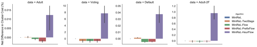
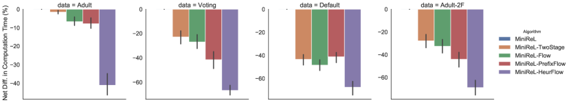
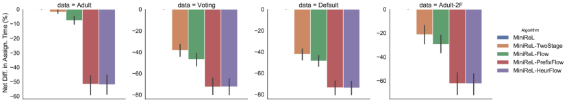
Figure 4: Impact of algorithmic components on cluster quality, computation time and average time to solve assignment problem in $k$-means setting. Amounts are normalized to show the percent change with respect to the base MiniReL algorithm that solves the full FMRA problem at each iteration, and averaged over $k\in[2,14]$. Negative values indicate an improvement over the base algorithm. Bars report the standard error.

4.1 Comparing different variants of the MiniReL

We evaluate the following 5 different variants of the MiniReL algorithm to show the impact of different algorithmic components on its performance:

• MiniReL: The baseline algorithm that solves the full FMRA at each iteration.

• MiniReL-TwoStage: Decomposes the FMRA by sequentially solving the RAP , by relaxing the $z$ variables and solving the problem via IP, and APFRC , using IP.

• MiniReL-TwoStageFlow: Uses the two-stage decomposition and solves the second stage using the network flow approach introduced in section 3.2.

• MiniReL-PrefixFlow: Uses the two-stage decomposition with pre-fixing (i.e., solves the RAP via IP once) and solves the second stage using the network flow approach introduced in section 3.2.

• MiniReL-PrefixHeurFlow: Uses the two-stage decomposition with pre-fixing with the polynomial time heuristic introduced in section 3.1 and solves the second stage using the network flow approach introduced in section.

For the sake of brevity we report results for this ablation study in the $k$-means setting, but the results were similar in the $k$-medians setting. Figure 4 shows the performance of these five different variants with respect to cluster quality, computation time, and average time to solve the assignment stage of the algorithm. All the amounts presented are normalized to show the percent change with respect to the base MiniReL algorithm, and averaged over $k\in[2,14]$. Negative values indicate an improvement over the baseline algorithm. Overall, the results show that the two-stage decomposition (MiniReL-TwoStage) approach leads to a decrease in computation time over the baseline algorithm leading to as much as a 20% percentage reduction in computation time on the Adult data set with two sensitive features. Solving the second stage problem via network flow (MiniReL-TwoStageFlow) also gives a small additional reduction in computation time over the the two-stage decomposition alone. Both approaches have no large impact on the objective (i.e., clustering cost) of the final solutions). Adding pre-fixing (Minirel-PrefixFlow) while still solving the RAP problem via IP yields an additional reduction in computation time in most of the datasets - the exception being the Default that had on average only 1.2 iterations that needed to use IP. Solving the RAP problem via the polynomial time heuristic led to a large additional reduction in computation time (an additional 30% in the adult dataset) but comes with a slight reduction to the quality of the clusters found. In most datasets this increase in cluster cost is small (under 1% on average) but in the voting dataset this led to a 7% point increase.

4.2 k-means results

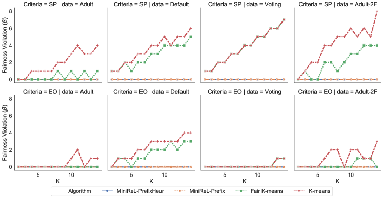
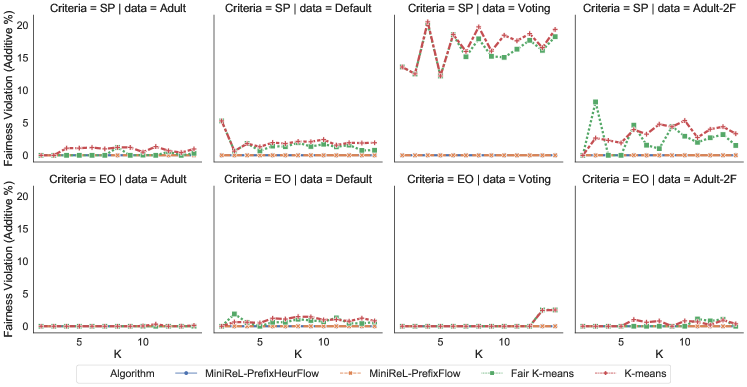
Figure 5: (Top 2 Rows) Maximum deviation from $\beta_{g}$ for Lloyd’s algorithm and MiniReL with IP assignment in $k$-means setting under both notions of fairness. (Bottom 2 Rows) Normalized Additive Fairness Violation (additive fairness violation divided by dataset size) for Lloyd’s algorithm and MiniReL with network flow assignment under both notions of fairness.

We compare the full version of MiniReL with heuristic pre-fixing and network flow assignment in the $k$-means setting with the standard Lloyd’s algorithm for $k$-means. We evaluate both algorithms with respect to cluster statistical parity (i.e., every group must be $\alpha$-represented in the same number of clusters), and cluster equality of opportunity (i.e., every every group must be $\alpha$-represented in a number of clusters proportional to the size of the group).

Figure 5 (top 2 rows) shows the maximum deviation from the fairness parameters $\beta_{g}$ (i.e., $\max_{g}\max(\beta_{g}-\Lambda(C,X_{g},\alpha),0)$) for the k-means algorithms and the variants of MiniReL that use IP to strictly enforce fairness. Figure 5 (bottom 2 rows) shows the total additive fairness violation normalized by the size of the dataset for the k-means algorithms and the variant of MiniReL that uses network flow to approximately enforce fairness. Across all three datasets we can see that $k$-means can lead to outcomes that violate MR-fairness constraints significantly, and that selecting the fairest clustering has only marginal improvement. This is most stark in the default dataset where there is as much as an 11 cluster gap (6 cluster fairness violation) between the two groups despite having similar proportions in the dataset. In contrast, the MiniReL algorithm is able to generate fair clusters under both notions of fairness and for all three datasets. This result also applies in the additive fairness violation setting, where the k-means algorithms generate large constraint violations (as much as 20% of the dataset size for the voting dataset) whereas the MiniReL algorithms with flow assignment have normalized additive fairness violations close to 0%. Table 1 shows the average computation time in seconds for Lloyd’s algorithm and MiniReL-PrefixHeurFlow under cluster statistical parity. We display results for the cluster statistical parity as it was the more computationally demanding setting requiring more MiniReL iterations than cluster equality of opportunity. As expected, the harder assignment problem in MiniReL leads to higher overall computation times when compared to the standard Lloyd’s algorithm. However, MiniReL is still able to solve large problems in under 200 seconds demonstrating that the approach is of practical use.

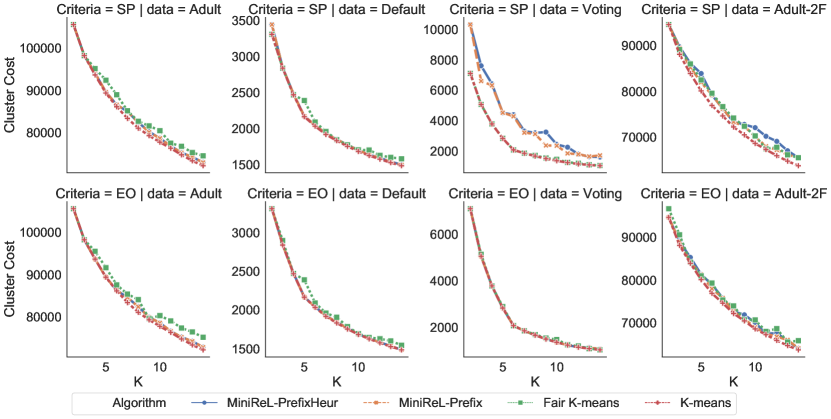
Figure 6: $k$-means clustering cost of Lloyd’s algorithm and MiniReL.

One remaining question is whether fairness comes at the expense of the cost of the clustering. Figure 6 shows the $k$-means clustering cost for Lloyd’s algorithm and MiniReL under both definitions of fairness. Although there is a small increase in the cost when using MiniReL the overall cost closely matches that of the standard $k$-means algorithm in 5 out of 6 instances, with the sole exception being the voting dataset under statistical parity, showing that we can gain fairness at practically no additional increase to clustering cost.

Table 1: Average computation time (standard deviation) in seconds for MiniReL-PrefixHeurFlow under Statistical Parity in the $k$-means setting. Final row includes average computation time over all settings of K for each dataset.

. data Adult Adult-2F Default Voting k K-means MiniReL K-means MiniReL K-means MiniReL K-means MiniReL 2 2.38 (0.28) 4.07 (0.35) 2.76 (0.49) 4.03 (0.26) 0.7 (0.08) 7.8 (2.34) 0.6 (0.14) 29.11 (3.37) 3 2.47 (0.19) 4.66 (0.69) 2.93 (0.67) 10.45 (3.27) 0.99 (0.27) 4.03 (1.03) 0.72 (0.1) 67.39 (89.39) 4 2.59 (0.12) 10.11 (2.06) 3.24 (0.64) 31.34 (14.36) 1.17 (0.27) 4.39 (1.27) 1.1 (0.33) 72.44 (20.78) 5 2.76 (0.24) 9.72 (2.02) 3.52 (0.68) 27.02 (11.7) 1.35 (0.42) 5.03 (1.9) 1.17 (0.33) 50.19 (16.16) 6 2.94 (0.27) 11.62 (2.57) 3.72 (0.74) 47.13 (39.03) 1.49 (0.32) 4.96 (1.37) 1.09 (0.2) 133.03 (58.33) 7 3.13 (0.33) 11.4 (0.77) 3.98 (0.81) 36.94 (18.13) 1.89 (0.79) 5.34 (1.39) 1.19 (0.22) 64.99 (37.16) 8 3.38 (0.28) 12.46 (3.7) 4.38 (0.78) 37.82 (19.45) 2.26 (0.67) 5.39 (0.64) 1.58 (0.36) 152.75 (118.6) 9 3.55 (0.51) 12.95 (3.58) 4.38 (0.77) 46.91 (18.71) 2.1 (0.67) 5.62 (0.43) 1.87 (0.42) 95.03 (82.51) 10 4.11 (0.53) 13.37 (2.95) 4.17 (0.75) 56.99 (31.76) 2.21 (0.75) 6.09 (0.61) 1.97 (0.61) 99.07 (83.35) 11 4.17 (0.57) 14.9 (3.88) 4.93 (2.34) 55.57 (17.95) 2.43 (0.67) 6.5 (1.13) 2.34 (0.85) 170.01 (82.46) 12 4.01 (0.43) 15.2 (2.36) 5.54 (2.11) 66.25 (31.31) 2.77 (0.82) 6.62 (0.44) 2.48 (0.61) 95.17 (25.11) 13 4.39 (0.5) 15.18 (3.89) 6.36 (2.41) 71.58 (35.91) 3.04 (0.96) 7.2 (1.06) 2.78 (0.67) 197.8 (51.53) 14 4.49 (0.58) 15.91 (5.23) 5.01 (5.74) 57.52 (15.32) 3.34 (1.11) 7.65 (1.26) 2.93 (0.69) 158.76 (42.36) mean 3.44 13.31 3.8 42.04 1.78 7.73 1.57 163.15

4.3 k-medians results

In this section we benchmark MiniReL against the Lloyd-style $k$-medians algorithm Park and Jun, (2009). The results closely parallel those in the $k$-means section and thus in the interest of brevity we present a subset of results for the algorithm under statistical parity and include the extended results in Appendix H. Figure 7 shows the maximum fairness violation and normalized additive fairness violation for MiniReL and the baseline $k$-medians algorithm. Similar to the $k$-means setting, the $k$-medians algorithm without fairness constraints can lead to unfair outcomes across all datasets, whereas MiniReL constructs fair clusters by design. Figure 8 shows the cluster cost for both algorithms in the same setting. Adding fairness in these settings again leads to only moderate increase in cluster cost, with the only notable increase coming on the voting dataset under statistical parity. Table 2 shows the runtime of both algorithms under statistical parity. MiniReL still leads to a modest increase in runtime compared to the baseline algorithm but is able to solve all datasets (10,000 data points after sub-sampling) in under 60 seconds in most instances.

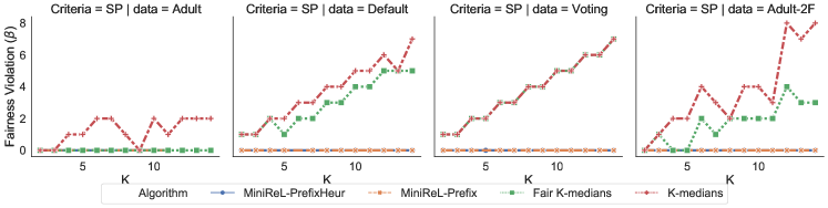
Figure 7: Maximum deviation from $\beta_{g}$ for Lloyd’s algorithm and MiniReL in $k$-medians setting with IP assignment under Statistical Parity.

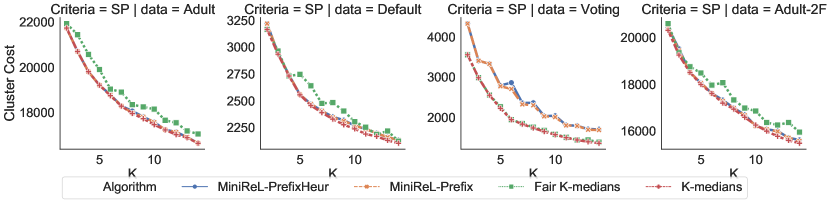
Figure 8: $k$-medians clustering cost of Lloyd’s algorithm and MiniReL under statistical parity.

Table 2: Average computation time (standard deviation) in seconds for MiniReL-PrefixHeurFlow under Statistical Parity in $k$-medians setting. Final row includes average computation time over all settings of K for each dataset. Note all datasets are sub-sampled to 10,000 points

. data Adult Adult-2F Default Voting k K-medians MiniReL K-medians MiniReL K-medians MiniReL K-medians MiniReL 2 2.5 (0.87) 7.77 (0.9) 2.72 (1.29) 8.17 (2.32) 3.46 (1.14) 9.73 (1.92) 7.03 (2.44) 16.24 (3.38) 3 2.52 (0.46) 7.43 (0.64) 3.98 (1.45) 9.03 (1.25) 2.58 (0.4) 7.37 (0.97) 8.2 (2.23) 15.33 (3.32) 4 2.76 (0.4) 7.11 (0.59) 3.04 (1.19) 8.01 (1.25) 3.32 (0.99) 8.55 (2.16) 10.7 (4.9) 18.79 (5.69) 5 2.8 (0.55) 7.1 (0.94) 3.58 (2.67) 7.96 (2.94) 3.09 (0.44) 7.91 (1.26) 14.27 (10.95) 31.64 (14.15) 6 2.93 (0.6) 7.29 (0.62) 4.36 (2.57) 8.97 (2.27) 3.1 (0.3) 8.11 (0.96) 13.27 (5.87) 20.23 (3.24) 7 2.93 (0.78) 7.27 (0.56) 3.58 (1.79) 7.66 (1.16) 3.57 (1.43) 8.49 (1.28) 12.05 (7.75) 16.96 (4.47) 8 2.99 (0.89) 7.69 (0.79) 3.74 (1.84) 8.2 (1.7) 3.48 (1.84) 8.65 (2.4) 36.0 (84.44) 22.16 (7.55) 9 3.01 (1.1) 7.61 (0.39) 5.01 (2.86) 8.81 (2.74) 4.27 (3.45) 9.03 (2.78) 25.45 (26.51) 27.1 (12.65) 10 3.49 (1.61) 8.15 (1.06) 5.5 (3.54) 10.09 (3.52) 4.68 (4.65) 8.22 (1.29) 24.76 (34.03) 23.84 (6.25) 11 3.31 (1.44) 8.18 (0.84) 5.6 (3.86) 11.42 (3.92) 3.76 (1.43) 8.36 (0.94) 31.0 (57.99) 29.17 (10.21) 12 3.48 (1.53) 8.57 (1.1) 5.68 (3.49) 9.72 (1.95) 3.63 (1.38) 8.8 (1.38) 20.23 (15.83) 25.84 (7.77) 13 3.53 (1.58) 8.71 (1.02) 6.04 (3.87) 11.04 (3.52) 5.04 (3.67) 10.38 (3.51) 30.36 (59.47) 29.45 (15.25) 14 3.74 (1.64) 9.15 (1.29) 6.58 (4.2) 12.0 (3.84) 4.2 (2.22) 9.17 (1.48) 64.83 (115.41) 39.16 (15.45) mean 2.97 7.35 1.91 11.37 2.64 8.65 13.45 19.63

5 Conclusion

In this this paper we introduce a novel definition of group fairness for clustering that requires each group to have a minimum level of representation in a specified number of clusters. This definition is a natural fit for a number of real world examples, such as voting and entertainment segmentation. To create fair clusters we introduce a modified version of Lloyd’s algorithm called MiniReL that solves an assignment problem in each iteration via integer programming. While solving the integer program remains a computational bottleneck, we note that our approach is able to solve problems of practical interest, including datasets with tens of thousands of data points, and provides a mechanism to design fair clusters when Lloyd’s algorithm fails.

Appendix A Proof of Theorem 1

Proof.

Proof The reduction is from the exact cover by 3 sets (X3C) problem, with $3q$ elements ${\cal U}=\{u_{1},\dots,u_{3q}\}$ and $t=q+r$ subsets ${\cal W}=\{W_{1},\dots,W_{t}\}$ where each subset $W_{i}\subseteq{\cal U}$ and $|W_{i}|=3$. Recall that X3C is one of Karps 21 NP-Complete problems and its goal is to select a collection of subsets ${\cal W}^{*}\subseteq{\cal W}$ such that all elements of ${\cal U}$ are covered exactly once.

Given an instance of the X3C problem, we first construct an undirected bipartite graph $G=({{\cal U}\cup{\cal W}},E)$ which we then convert into a FMRA instance following a similar construction as (Esmaeili et al.,, 2022). Graph $G$ has a node for each $u_{i}\in{\cal U}$ and a node $w_{j}$ for each $W_{j}\in{\cal W}$. There is an edge $\{u_{i},w_{j}\}$ between nodes $u_{i}$ and ${w_{j}}$ provided that $u_{i}\in W_{j}$. Note that with slight abuse of notation, we use ${\cal W}$ both for the subsets in the X3C instance and the nodes corresponding to them in the graph $G$.

Using graph $G$, we construct an instance of the FMRA problem with two groups by interpreting each vertex in the graph as a data point where points corresponding to vertices in ${\cal U}$ and ${\cal W}$ belong to separate groups. We set $K=t$ (i.e., one cluster for each subset), $\alpha=0.75$, $\beta_{W}=t-q$ and $\beta_{U}=q$ (minimum number of $\alpha$-represented clusters for each group). We place the (fixed) $K$ centers at the data points associated with $\cal W$. The distances between pairs of data points are set to be the length of the shortest path distances between the corresponding vertices in the graph.

We now argue that the optimal solution to the FMRA instance has a cost of $3q$ if and only if there exists a feasible solution to the X3C instance. First note that any feasible solution to the FMRA instance has a cost of at least $3q$ as each point $u_{i}\in{\cal U}$ incurs a cost of at least 1 and there are $3q$ such points. Next, note that given a feasible solution ${\cal W}^{*}\subseteq{\cal W}$ to the X3C instance, we can construct a solution to the corresponding FMRA instance with cost $3q$ by creating one cluster for each $W_{j}\in{\cal W}^{*}$ in the solution. These $q$ clusters contain $w_{j}$ together with the 3 elements $u_{i}\in W_{j}$. The remaining $t-q$ clusters contain a single point $w_{j}$, one for for each $W_{j}\in{\cal W}\setminus{\cal W}^{*}$. Note that these clusters satisfy the fairness constraints. Furthermore, letting the center of each cluster to be the $w_{j}$ that it contains gives a cost of $3q$.

Finally we argue that if the FMRA instance has a cost of $3q$, then the X3C instance is feasible. If the solution to the FMRA has cost $3q$, then $(i)$ each point $u_{i}\in{\cal U}$ must be assigned to a center $w_{j}\in{\cal W}$ such that $u_{i}\in W_{j}$, and, $(ii)$ each point $w_{j}\in{\cal W}$ must be assigned to the center $w_{j}$ and consequently, each cluster must contain exactly one $w_{j}\in{\cal W}$. In addition, the fairness constraint for the ${\cal W}$ group requires that at least $t-q$ clusters must have 75% of its points belonging to the ${\cal W}$ group. As there is exactly one $w_{j}\in{\cal W}$ in each cluster, this can only happen if at least $t-q$ clusters have no points from ${\cal U}$ group in them. Consequently all $3q$ points form the ${\cal U}$ group are assigned to at most $q$ clusters. As all $u_{i}\in{\cal U}$ must be assigned to a center $w_{j}\in{\cal W}$ such that $u_{i}\in W_{j}$, and $|W_{j}|=3$, the solution to the FMRA instance must have exactly $t-q$ clusters with no points from ${\cal U}$ group and $q$ clusters with one $w_{j}$ and three $u_{i}\in W_{j}$, which gives a feasible solution to the X3C instance. ∎∎

Appendix B Proof of Theorem 2

Proof.

Proof.We start by noting that given an assignment of data points to clusters, the optimal cluster centers for this assignment are precisely the ones computed as in Step 7 (9).Consequently, if improved_cost = current_cost in Step 13, then the cluster centers used in Step 3 and the ones computed in Step 7 or 9 (in the last iteration) must be identical. This follows from the uniqueness of the optimal centers in the $k$-means setting and the deterministic tie-breaking in the $k$-medians setting. Therefore, if Algorithm 1 terminates, then the current assignment of the data points to the current cluster centers is optimal and the cost cannot improve by changing their assignment due to Step 3. In addition, Steps 7 and 9 guarantees that perturbing cluster centers cannot not improve the cost for the current assignment.

It remains to show that the algorithm will terminate after a finite number of iterations. Similar to the proof for Lloyd’s algorithm, we leverage the fact that there are only a finite number of partitions of the data points. By construction, the objective value decreases in each iteration of the algorithm, and thus can never cycle through any partition multiple times as for a given partition we use the optimal cluster centers when computing improved_cost in Step 12. Thus the algorithm can visit each partition at most once and thus must terminate in finite time. ∎

∎

Appendix C Proof of Theorem 4

Proof.

Proof Given an instance of a 3-SAT problem, one of Karp’s 21 NP-Complete problems, we construct an instance of the APFRC problem as follows. We start with a 3-SAT problem with $n$ variables and $m$ clauses $K_{1},\dots,K_{m}$. Each clause $K_{i}$ takes the form $v_{i1}\vee v_{i2}\vee v_{i3}$ where $v_{ij}$ is either one of the original variables or its negation.

To construct the instance of the APFRC problem, start by creating two new data points $x_{v_{i}},x_{\bar{v}_{i}}$, corresponding to each original variable $v_{i}$ and its negation respectively. We construct two clusters $C_{1}$ and $C_{2}$ that each variable can be assigned to. Let ${\cal W}$ represent the set of allowable group-cluster assignments (i.e., $(g,k)\in{\cal W}$ if $y_{gk}=1$). For each original variable $v_{i}$ we create one group $g_{i}=\{x_{v_{i}},x_{\bar{v}_{i}}\}$ that can be $\alpha$-represented in either cluster (i.e. $(g_{i},1),(g_{i},2)\in\mathcal{W}$). For each group $g_{i}$ we set $\beta_{g_{i}}=2$ - ensuring that both clusters must be $\alpha$-represented by the group. We also create one group for each clause $K_{i}$ corresponding to its three conditions $g_{K_{i}}=\{x_{v_{i1}},x_{v_{i2}},x_{v_{i3}}\}$ that must be $\alpha$-represented in cluster $1$ (i.e. $(g_{K_{i}},1)\in\mathcal{W},(g_{K_{i}},2)\notin\mathcal{W}$). For these groups we set $\beta_{K_{i}}=1$. Finally, we set $\alpha=\frac{1}{2n}$ - this ensures that any assignment of a group’s data point to a cluster will satisfy the $\alpha$-representation constraint (as there are $2n$ data points and thus at most $2n$ data points in a cluster). We also add a cardinality lower bound on both clusters of 1. Clearly the above scheme can be set-up in polynomial time.

We now claim that a feasible solution to the aforementioned APFRC problem corresponds to a solution to the original 3-SAT instance. We start by taking the variable settings by looking at $C_{1}$. We start by claiming that for each variable exactly one of $x_{v_{i}},x_{\bar{v}_{i}}$ are included in $C_{1}$. Suppose this weren’t true, either both variables were included in $C_{1}$ or $C_{2}$. However, whichever cluster has neither of the variables would not be $\alpha$-represented by group $g_{i}$, thereby contradicting the fairness constraints. Since $C_{1}$ contains either $x_{v_{i}}$ or $x_{\bar{v}_{i}}$ we set $v_{i}=T$ if $x_{v_{i}}$ is included and $v_{i}=F$ otherwise. We now claim that such a setting of the variables satisfies all the clauses. Assume it did not, then there exists a clause $K_{i}$ such that none of $x_{v_{i1}},x_{v_{i2}},x_{v_{i3}}$ are included in $C_{1}$. However, this violates the $\alpha$-representation constraint for $g_{K_{i}}$ providing a contradiction to the feasibility of the fair assignment problem. Note that since the feasibility problem does not consider the objective or the location of the centers the proof applies for both the $k$-means and $k$-medians setting. ∎

Appendix D Experiments with different objectives for RAP heuristic

To test the efficacy of the myopic cost for pre-fixing we perform a computational study. We experiment with three different choices of cost function:

• Proportion: Set the cost to the proportion of the cluster that needs to be changed for $g$ to be $\alpha$-represented in cluster $k$:

  $$c_{gk}=\max(\alpha-p_{gk},0)$$

  where $p_{gk}$ is the current proportion of cluster $k$ that belongs to group $g$.

• Weighted Proportion: Set the cost to the proportion weighted by the size of the cluster:

  $$c_{gk}=|C_{k}|\max(\alpha-p_{gk},0).$$

• Local Cost: The myopic (i.e. one-shot) increase in cost of moving additional data points to cluster $k$ to meet the fairness constraints. Let $q$ be the additional number of points from group $g$ needed for $g$ to be $\alpha$-represented in this cluster (i.e. $q+p_{gk}|C_{k}|\geq\alpha(q+|C_{k}|)$). Let $c_{(x)}=\operatorname{\arg\min}_{c\in\{c_{1},\dots,c_{K}\}}\{D(x,c)\}$ be the closest center for $x\in{\cal X}$. The myopic cost $c_{gk}$ associated with $\alpha$-representing group $g$ in cluster $k$ then becomes:

  $$c_{gk}=\min_{X\subset X_{g}\setminus C_{K}:|X|=q}\sum_{x\in X}\big{(}D(x,c_{k})-D(x,c_{(x)})\big{)}$$

Figure 9 shows the impact of different choices of the objective in IP model (8)-(11) on run-time for MiniReL on three different datasets. For these experiments we focused on the $k$-means setting (though $k$-medians showed a similar result) and ran 10 trials with different random initial seeds, and warm-start the algorithm with the standard Lloyd’s algorithm. We benchmark using the IP model to perform pre-fixing with naively pre-fixing the group cluster assignments (i.e. random assignment). In the small 150 data point iris dataset, the pre-fixing scheme has little impact on the total run-time of the algorithm as the overhead of running the IP model outweighs any time savings from a reduced number of iterations. However, for larger datasets (i.e. adult and default which both have over 30K data points), using the IP model to perform pre-fixing outperforms the naive approach - leading to as large as a 3x speed-up. However, there is a relatively small difference in performance between the three choices for the objective, with the local cost objective reducing the speed by approximately $0.1\%$ compared to the other two when averaged across all three datasets.

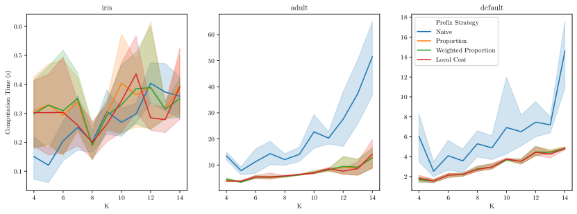
Figure 9: Impact of pre-fixing strategy on the run-time of the MiniReL algorithm. Proportion, Weighted Proportion, and Local Cost are pre-fixing strategies that use the pre-fix IP model with different objectives. Naive denotes random assignments of groups to clusters. Results averaged over 10 random seeds, widths indicate standard error.

Figure 10 shows the impact of pre-fixing strategy on the number of iterations needed for MiniReL to converge. For iris, pre-fixing has practically no impact on on the number of iterations, however for larger datasets like adult and default using the pre-fix IP model with any objective leads to substantially fewer iterations. The same holds for cluster cost as shown in Figure 11 where the IP model leads to solutions with slightly better clustering cost in both adult and default. Both results show that the choice of objective function has relatively little impact on the performance of pre-fixing, but outperform random assignment.

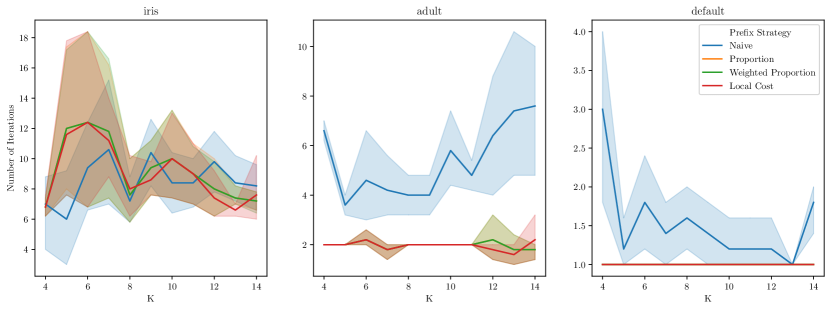
Figure 10: Impact of pre-fixing strategy on the on the number of iterations to convergence for MiniReL. Results averaged over 10 random seeds. Bars indicate standard error.

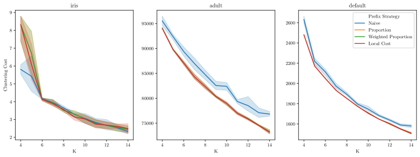
Figure 11: Impact of pre-fix strategy on the clustering cost of the solution output by MiniReL. Results averaged over 10 random seeds. Bars indicate standard error.

Appendix E Warm-Starting MiniReL

To reduce the number of iterations needed to converge in MiniReL, we warm-start the initial cluster centers with the final centers of the unfair variants of Lloyd’s algorithm. The key intuition behind this approach is that it allows us to leverage the polynomial time assignment problem for the majority of iterations, and only requires solving the fair assignment problem to adjust the locally optimal unfair solution to a fair one. To incorporate warm-starting into MiniReL, we replace step 1 in Algorithm (1) with centers generated from running Lloyd’s algorithm. For the sake of brevity, we report results in the $k$-means setting. We benchmark this approach against two baselines: $(i)$ randomly sampling the center points, and $(ii)$ using the $k$-means++ initialization scheme without running Lloyd’s algorithm afterwards. We also compare using the $k$-means warm-start with 1 initialization and 100 initializations. Figure 12 shows the impact of these initialization schemes on the total computation time including time to perform the initialization. Each initialization scheme was tested on three datasets. For each dataset we randomly sub-sample 2000 data points (if $n>2000$), and re-run MiniReL with 10 random seeds. The results show that using Lloyd’s algorithm to warm-start MiniReL can lead to a large reduction in computation time, even taking into account the cost of running the initialization. However, there are diminishing returns. Namely running 100 different initialization for $k$-means and selecting the best leads to slightly larger overall run-times.

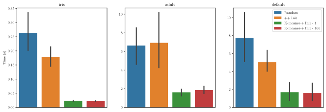
Figure 12: Average computation time in seconds over 10 random seeds for MiniReL with different initialization schemes. Bars indicate standard error.

Appendix F Experiments with different values of $\alpha$

In this section we explore the impact of $\alpha$ on the fairness and runtime of the different algorithms. For these experiments we replicate the experimental set-up of Section 4.2 but vary $\alpha$. For brevity we focus on the $k$-means setting, but $k$-medians showed similar results. Figures 13 and 14 show the normalized fairness violation (the number of $\alpha$-represented clusters away from meeting the required amount $\beta_{g}$ normalized by $K$) and normalized additive fairness violation (the number of data points away from meeting the fairness constraints normalized by $n$). In both cases, lower value of $\alpha$ lead to much laxer fairness requirements that are easier to meet. Both the standard $k$-means and the heuristic fair $k$-means algorithms are able to generate fair clusters for $\alpha\leq 0.3$ for both statistical parity and equality of opportunity settings of $\beta_{g}$. However for larger values of $\alpha$ both struggle to generate fair clusters having normalized (additive) violations close to 100% (25%). In constrast, by design MiniReL with IP-based assignment (MiniRel-Prefix) is able to generate fair clusters at all levels of $\alpha$. While the version of MiniReL with network flow rounding (MiniReL-PrefixFlow) can lead to fairness violations, the size of the violations are consistently small (in line with our theoretical results) - violating the constraints by close to 0% of the size of the dataset. Figure 15 shows the impact of $\alpha$ and $K$ on the computation time of all algorithms. As expected, both $k$-means and fair $k$-means run very quickly regardless of $K$ (and $\alpha$ evidently has no impact on the runtime). In contrast, the runtime of MiniReL increases with both $K$ and $\alpha$ showing that harder assignment problems lead to larger runtimes overall.

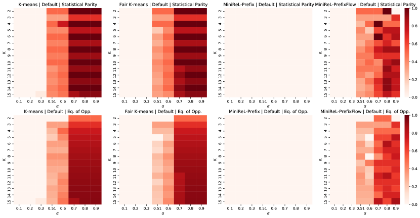
Figure 13: Impact of $\alpha$ and $K$ on the normalized fairness violation $\max_{g}\max(\beta_{g}-\Lambda(C,X_{g},\alpha),0)/K$. Higher values (closer to one) indicate larger fairness violations.

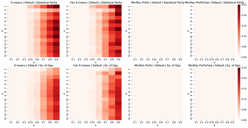
Figure 14: Impact of $\alpha$ and $K$ on the normalized additive fairness violation (normalized by number of data points). Higher values (closer to one) indicate larger fairness violations.

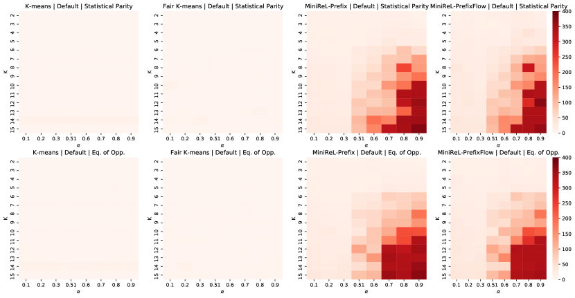
Figure 15: Impact of $\alpha$ and $k$ on the runtime (s) of the different algorithms.

Appendix G Experiments with balanced clusters

In this section we explore the impact of constructing balanced clusters (i.e., clusters with approximately equal size) on the objective and computation time of MiniReL. For these experiments we require each cluster to have at least 80% of the balanced allocation of data points to clusters (i.e., $\ell=0.8*\frac{n}{K}$. Figure 16 shows the $k$-means clustering cost of both Lloyd’s algorithm (with no cardinality constraints) and the cost of MiniReL with balanced clusters. The first thing to note is that under balanced clusters, not every dataset and setting for $\alpha$, $\beta$ remains feasible. For the voting dataset under statistical parity, MiniReL certifies that no fair clustering exists (and thus has no associated objective or runtime). Overall, requiring balance leads to a modest increase in cluster cost across all instances - exceeding the deviation that occurs from enforcing fairness alone. Table 3 shows the average runtime over 10 random seeds for $K$-Means and MiniReL-HeurFlow under balanced clusters for statistical parity. Adding the requirement that clusters are balanced leads to a small increase in runtime for MiniReL on all datasets. The one exception is the voting dataset, which is an infeasible problem, where MiniReL can certify infeasibility in under 30 seconds for all settings of $K$.

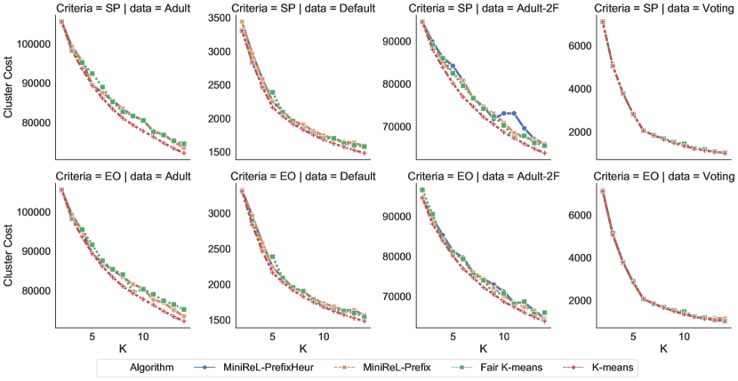
Figure 16: $k$-means clustering cost of Lloyd’s algorithm and MiniReL with balanced clusters.

Table 3: Average computation time in seconds for MiniReL-HeurFlow under Statistical Parity with balanced clusters. Final row includes average computation time over all settings of K for each dataset.

. data Adult Adult-2F Default Voting k K-means MiniReL K-means MiniReL K-means MiniReL K-means MiniReL 2 2.22 9.41 3.04 8.80 0.65 11.21 0.48 8.64 3 2.40 15.08 3.03 13.47 0.82 11.72 0.56 9.23 4 2.80 26.29 3.00 27.71 0.79 12.79 1.30 10.24 5 2.58 18.27 3.59 30.41 1.25 13.85 0.84 13.31 6 2.87 19.00 2.65 22.79 1.42 15.03 0.92 13.22 7 3.10 39.18 3.66 23.63 2.36 16.10 1.07 14.37 8 3.08 41.11 5.70 25.51 1.50 17.83 1.48 15.27 9 3.15 29.61 6.07 76.04 1.53 18.57 1.53 13.64 10 4.57 31.00 6.33 70.21 1.88 20.45 2.76 15.12 11 4.02 24.87 3.79 46.01 2.01 33.05 1.90 15.94 12 3.53 42.30 5.24 72.27 2.66 34.49 2.93 17.71 13 4.09 36.90 4.08 81.45 3.21 30.42 3.23 23.77 14 4.33 27.62 2.91 46.12 8.42 24.61 3.21 22.37 mean 3.29 27.74 4.08 41.88 2.19 20.01 1.71 14.83

Appendix H Full $k$-medians results

The following section includes the extended empirical results for MiniReL in the $k$-medians section. Figure 17 shows both the maximum fairness violation and normalized additive fairness violation of both algorithms under both notions of fairness. Regardless of the setting, the baseline $k$-medians algorithm and its fair heuristic analog are unable to generate fair clusters - whereas MiniReL can construct fair clusters or clusters with negligible additive fairness violations by design. Figure 18 shows the clustering objective of both sets of algorithms. With the exception of the voting dataset under statistical parity, MiniReL is able to generate fair clusters with practically no increase in the cluster cost - showing that in practical settings achieving minimum representation fairness comes at little cost over Lloyd’s algorithm.

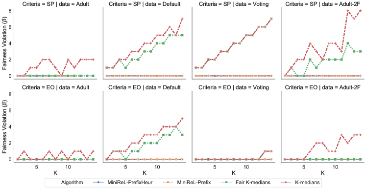
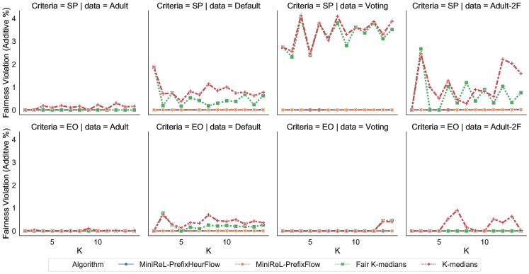
Figure 17: (Top 2 Rows) Maximum deviation from $\beta_{g}$ for Lloyd’s algorithm and MiniReL in the $k$-medians setting with IP assignment under both notions of fairness. (Bottom 2 Rows) Normalized Additive Fairness Violation (additive fairness violation divided by dataset size) for Lloyd’s algorithm and MiniReL with network flow assignment under both notions of fairness.

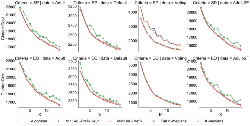
Figure 18: $k$-medians clustering cost of Lloyd’s algorithm and MiniReL.

References

- Abbasi et al., (2021) Abbasi, M., Bhaskara, A., and Venkatasubramanian, S. (2021). Fair clustering via equitable group representations. In Proceedings of the 2021 ACM Conference on Fairness, Accountability, and Transparency, pages 504–514, New York. ACM.
- Ahmadian et al., (2020) Ahmadian, S., Epasto, A., Knittel, M., Kumar, R., Mahdian, M., Moseley, B., Pham, P., Vassilvitskii, S., and Wang, Y. (2020). Fair hierarchical clustering. Advances in Neural Information Processing Systems, 33:21050–21060.
- Ahmadian et al., (2019) Ahmadian, S., Epasto, A., Kumar, R., and Mahdian, M. (2019). Clustering without over-representation. In Proceedings of the 25th ACM SIGKDD International Conference on Knowledge Discovery & Data Mining, pages 267–275, New York. ACM.
- Backurs et al., (2019) Backurs, A., Indyk, P., Onak, K., Schieber, B., Vakilian, A., and Wagner, T. (2019). Scalable fair clustering. In International Conference on Machine Learning, pages 405–413, Long Beach, California USA. PMLR, PMLR.
- Bandyapadhyay et al., (2020) Bandyapadhyay, S., Fomin, F. V., and Simonov, K. (2020). On coresets for fair clustering in metric and euclidean spaces and their applications. arXiv:2007.10137.
- Benade et al., (2022) Benade, G., Ho-Nguyen, N., and Hooker, J. (2022). Political districting without geography. Operations Research Perspectives, 9:100227.
- Bera et al., (2019) Bera, S., Chakrabarty, D., Flores, N., and Negahbani, M. (2019). Fair algorithms for clustering. In Wallach, H., Larochelle, H., Beygelzimer, A., d'Alché-Buc, F., Fox, E., and Garnett, R., editors, Advances in Neural Information Processing Systems, volume 32, Vancouver, CA. Curran Associates, Inc.
- Bercea et al., (2018) Bercea, I. O., Groß, M., Khuller, S., Kumar, A., Rösner, C., Schmidt, D. R., and Schmidt, M. (2018). On the cost of essentially fair clusterings. arXiv:1811.10319.
- Böhm et al., (2020) Böhm, M., Fazzone, A., Leonardi, S., and Schwiegelshohn, C. (2020). Fair clustering with multiple colors. arXiv:2002.07892.
- Brownwell, (2015) Brownwell, C. (2015). Crtc relaxes quotas on canadian content for tv broadcasters.
- Buolamwini and Gebru, (2018) Buolamwini, J. and Gebru, T. (2018). Gender shades: Intersectional accuracy disparities in commercial gender classification. In Conference on fairness, accountability and transparency, pages 77–91, New York City, USA. PMLR, PMLR.
- Chhabra et al., (2020) Chhabra, A., Vashishth, V., and Mohapatra, P. (2020). Fair algorithms for hierarchical agglomerative clustering. arXiv:2005.03197.
- Chierichetti et al., (2017) Chierichetti, F., Kumar, R., Lattanzi, S., and Vassilvitskii, S. (2017). Fair clustering through fairlets. In Guyon, I., Luxburg, U. V., Bengio, S., Wallach, H., Fergus, R., Vishwanathan, S., and Garnett, R., editors, Advances in Neural Information Processing Systems, volume 30, Long Beach, USA. Curran Associates, Inc.
- Chiplunkar et al., (2020) Chiplunkar, A., Kale, S., and Ramamoorthy, S. N. (2020). How to solve fair k-center in massive data models. In International Conference on Machine Learning, pages 1877–1886, Remote. PMLR, PMLR.
- Conforti et al., (2014) Conforti, M., Cornuéjols, G., Zambelli, G., et al. (2014). Integer Programming, volume 271. Springer.
- Daudpota et al., (2019) Daudpota, S. M., Muhammad, A., and Baber, J. (2019). Video genre identification using clustering-based shot detection algorithm. Signal, Image and Video Processing, 13(7):1413–1420.
- Dua et al., (2017) Dua, D., Graff, C., et al. (2017). Uci machine learning repository.
- Esmaeili et al., (2021) Esmaeili, S., Brubach, B., Srinivasan, A., and Dickerson, J. (2021). Fair clustering under a bounded cost. Advances in Neural Information Processing Systems, 34:14345–14357.
- Esmaeili et al., (2020) Esmaeili, S., Brubach, B., Tsepenekas, L., and Dickerson, J. (2020). Probabilistic fair clustering. Advances in Neural Information Processing Systems, 33:12743–12755.
- Esmaeili et al., (2022) Esmaeili, S. A., Duppala, S., Dickerson, J. P., and Brubach, B. (2022). Fair labeled clustering. In Proceedings of the 28th ACM SIGKDD Conference on Knowledge Discovery and Data Mining, pages 327–335.
- Ghadiri et al., (2021) Ghadiri, M., Samadi, S., and Vempala, S. (2021). Socially fair k-means clustering. In Proceedings of the 2021 ACM Conference on Fairness, Accountability, and Transparency, pages 438–448, Online. ACM.
- Goyal and Jaiswal, (2021) Goyal, D. and Jaiswal, R. (2021). Tight fpt approximation for socially fair clustering. arXiv:2106.06755.
- Gurnee and Shmoys, (2021) Gurnee, W. and Shmoys, D. B. (2021). Fairmandering: A column generation heuristic for fairness-optimized political districting. In SIAM Conference on Applied and Computational Discrete Algorithms (ACDA21), pages 88–99, Virtual. SIAM, SIAM.
- Gurobi Optimization, LLC, (2022) Gurobi Optimization, LLC (2022). Gurobi Optimizer Reference Manual.
- Harb and Lam, (2020) Harb, E. and Lam, H. S. (2020). Kfc: A scalable approximation algorithm for - center fair clustering. Advances in neural information processing systems, 33:14509–14519.
- Huang et al., (2019) Huang, L., Jiang, S., and Vishnoi, N. (2019). Coresets for clustering with fairness constraints. Advances in Neural Information Processing Systems, 32.
- Jain et al., (1999) Jain, A. K., Murty, M. N., and Flynn, P. J. (1999). Data clustering: a review. ACM computing surveys (CSUR), 31(3):264–323.
- Jia et al., (2020) Jia, X., Sheth, K., and Svensson, O. (2020). Fair colorful k-center clustering. In Integer Programming and Combinatorial Optimization: 21st International Conference, IPCO 2020, London, UK, June 8–10, 2020, Proceedings, pages 209–222, London. Springer, Springer.
- Jones et al., (2020) Jones, M., Nguyen, H., and Nguyen, T. (2020). Fair k-centers via maximum matching. In International Conference on Machine Learning, pages 4940–4949, Virtual. PMLR, PMLR.
- Kansal et al., (2018) Kansal, T., Bahuguna, S., Singh, V., and Choudhury, T. (2018). Customer segmentation using k-means clustering. In 2018 international conference on computational techniques, electronics and mechanical systems (CTEMS), pages 135–139, Belgaum, India. IEEE, IEEE.
- (31) Kleindessner, M., Awasthi, P., and Morgenstern, J. (2019a). Fair k-center clustering for data summarization. In International Conference on Machine Learning, pages 3448–3457, Long Beach, USA. PMLR, PMLR.
- (32) Kleindessner, M., Samadi, S., Awasthi, P., and Morgenstern, J. (2019b). Guarantees for spectral clustering with fairness constraints. In International Conference on Machine Learning, pages 3458–3467, Long Beach, USA. PMLR, PMLR.
- Kueng et al., (2019) Kueng, R., Mixon, D. G., and Villar, S. (2019). Fair redistricting is hard. Theoretical Computer Science, 791:28–35.
- Lawless and Günlük, (2024) Lawless, C. and Günlük, O. (2024). Fair minimum representation clustering. In Dilkina, B., editor, Integration of Constraint Programming, Artificial Intelligence, and Operations Research, pages 20–37, Cham. Springer Nature Switzerland.
- Le Quy et al., (2021) Le Quy, T., Roy, A., Friege, G., and Ntoutsi, E. (2021). Fair-capacitated clustering. In EDM, Paris, France. EDM.
- Levin and Friedler, (2019) Levin, H. A. and Friedler, S. A. (2019). Automated congressional redistricting. Journal of Experimental Algorithmics (JEA), 24:1–24.
- Liu and Vicente, (2021) Liu, S. and Vicente, L. N. (2021). A stochastic alternating balance -means algorithm for fair clustering. arXiv:2105.14172.
- Makarychev and Vakilian, (2021) Makarychev, Y. and Vakilian, A. (2021). Approximation algorithms for socially fair clustering. In Conference on Learning Theory, pages 3246–3264, Boulder, USA. PMLR, PMLR.
- Mehrabi et al., (2019) Mehrabi, N., Morstatter, F., Saxena, N., Lerman, K., and Galstyan, A. (2019). A survey on bias and fairness in machine learning. arXiv:1908.09635.
- Mehrotra et al., (1998) Mehrotra, A., Johnson, E. L., and Nemhauser, G. L. (1998). An optimization based heuristic for political districting. Management Science, 44(8):1100–1114.
- NCSBE, (2020) NCSBE (2020). North carolina voter registration data. https://www.ncsbe.gov/results-data/voter-registration-data.
- Park and Jun, (2009) Park, H.-S. and Jun, C.-H. (2009). A simple and fast algorithm for k-medoids clustering. Expert systems with applications, 36(2):3336–3341.
- Pedregosa et al., (2011) Pedregosa, F., Varoquaux, G., Gramfort, A., Michel, V., Thirion, B., Grisel, O., Blondel, M., Prettenhofer, P., Weiss, R., Dubourg, V., Vanderplas, J., Passos, A., Cournapeau, D., Brucher, M., Perrot, M., and Duchesnay, E. (2011). Scikit-learn: Machine learning in Python. Journal of Machine Learning Research, 12:2825–2830.
- Ricca et al., (2013) Ricca, F., Scozzari, A., and Simeone, B. (2013). Political districting: from classical models to recent approaches. Annals of Operations Research, 204:271–299.
- Schmidt et al., (2018) Schmidt, M., Schwiegelshohn, C., and Sohler, C. (2018). Fair coresets and streaming algorithms for fair k-means clustering. arXiv:1812.10854.
- scikit-learn-extra development team, (2020) scikit-learn-extra development team, T. (2020). scikit-learn-extra: a python module for machine learning that extends scikit-learn.
- Thejaswi et al., (2021) Thejaswi, S., Ordozgoiti, B., and Gionis, A. (2021). Diversity-aware -median: Clustering with fair center representation. arXiv:2106.11696.
- Wang et al., (2020) Wang, Y., Zhao, Y., Therneau, T. M., Atkinson, E. J., Tafti, A. P., Zhang, N., Amin, S., Limper, A. H., Khosla, S., and Liu, H. (2020). Unsupervised machine learning for the discovery of latent disease clusters and patient subgroups using electronic health records. Journal of biomedical informatics, 102:103364.
- Williamson, (2019) Williamson, D. P. (2019). Network flow algorithms. Cambridge University Press.
- Xu and Wunsch, (2005) Xu, R. and Wunsch, D. (2005). Survey of clustering algorithms. IEEE Transactions on neural networks, 16(3):645–678.
- Ziko et al., (2021) Ziko, I. M., Yuan, J., Granger, E., and Ayed, I. B. (2021). Variational fair clustering. In Proceedings of the AAAI Conference on Artificial Intelligence, volume 35, pages 11202–11209, Virtual. AAAI.