Quantum wavepackets: Proofs (almost) without words

Abstract

We present a geometrical way of understanding the dynamics of wavefunctions in a free space, using the phase-space formulation of quantum mechanics. By visualizing the Wigner function, the spreading, shearing, the so-called “negative probability flow” of wavefunctions, and the long-time asymptotic dispersion, are intuited visually. These results are not new, but previous derivations were analytical, whereas this paper presents elementary geometric arguments that are almost “proofs without words”, and suitable for a first course in quantum mechanics.

I Introduction

Phase-space quantum mechanics is a formulation of quantum mechanics that is mathematically equivalent to the standard ones (Schrödinger picture, Heisenberg picture, etc.), but offers a way of visualizing the dynamics of quantum systems that is closer to the classical intuition. In it, instead of wavefunctions that are vectors in a Hilbert space, quantum states are represented by quasiprobability distributions in phase space, called Wigner functions.

This paper does not review phase-space quantum mechanics in detail, for which one may consult Refs Case, 2008; Curtright, Fairlie, and Zachos, 2014 and references therein. To understand the paper, one only needs to know a few things about phase-space quantum mechanics.

For any pure state with position-space wavefunction $\psi(t,q)$ in $\mathbb{R}^{n}$, its corresponding Wigner quasiprobability function is defined as

$$W(t,q,p)=\frac{1}{(2\pi)^{n}}\int d^{n}ye^{-ip\cdot y}~{}\psi(t,q+y\hbar/2)\psi(t,q-y\hbar/2)^{*}$$ (1)

and for mixed states, the Wigner function is the linear sum of the Wigner functions of the pure states.

This allows us to calculate the probability density of finding a particle at a position in space $|\psi(t,q)|^{2}=\int_{\mathbb{R}}W(t,q,p)dp$ by integration, and similarly, also its momentum-space probability density $|\psi(t,p)|^{2}=\int_{\mathbb{R}}W(t,q,p)dq$.

The time-evolution is described by how $W(t,q,p)$ changes as $t$ increases, with a generalization of the classical Liouville equation:

$$\partial_{t}W=\{\{H,W\}\}$$

where $H(t,q,p)$ is a function, called the Hamiltonian of the system. Unlike the Hamiltonian operator in the Schrödinger picture, here the Hamiltonian is just a real-valued function.

If Hamiltonian $H$ is a sum of kinetic and potential energies, as $H=T(p)+V(q)$, and if both $T,V$ are quadratic polynomials, then one can show that $\partial_{t}W=\{H,W\}$, which is exactly the same as the classical Liouville equation of probability flow in phase space: $\partial_{t}\rho=\{H,\rho\}$, where $\rho$ is the (classical) probability density in phase space.

In other words, we can picture the phase-space evolution of such a Wigner function as if it is just the classical flow of probability density in phase space, as in classical statistical mechanics. The only difference is that there are both regions of positive and negative ”probability” densities (thus the name ”quasi-probability”).

There are essentially only three examples of such quadratic Hamiltonians. A particle in free space has Hamiltonian $H=\frac{\|p\|^{2}}{2m}$. Thus, the Wigner function $W$ evolves by a simple shearing flow in phase space:

$$W(t,q,p)=W(0,q-pt/m,p)$$

A particle under constant force $F$ has Hamiltonian $H=\frac{\|p\|^{2}}{2m}-F\cdot q$. Its Wigner function evolves by a parabolic translation in phase space:

$$W(t,q,p)=W(0,q-(Ft^{2})/(2m),p-Ft)$$

For example, in one dimensional space, the Airy wavepacket has a Wigner function whose contour lines are parabolas. Thus, with the right constant force, its Wigner function would remain unchanging.Berry and Balazs (1979) This makes it intuitively clear why the Airy wavepacket spontaneously accelerates, without dispersing.

Finally, a quantum harmonic oscillator in one dimension has Hamiltonian $H=\frac{p^{2}}{2m}+\frac{1}{2}m\omega^{2}q^{2}$, and so its Wigner function evolves by

$$W(t,q,p)=W\left(0,q\cos(\omega t)-\frac{p}{m\omega}\sin(\omega t),qm\omega\sin(\omega t)+p\cos(\omega t)\right)$$

Its generalization to $n$ dimensions is immediate.

II Particles in free space

II.1 Gaussian wavepacket

Consider the simplest case of a gaussian wavepacket on a line, centered at $q=0$, with zero total momentum. Over time, it contracts, until its width $\sigma_{q}$ reaches a minimum, before spreading out again. Let $t=0$ be the time of minimal width, so its wavefunction satisfies

$$\psi(0,q)=\sqrt{\rho_{N(0,\sigma_{q}^{2})}(q)}$$

where $\rho_{N(0,\sigma_{q}^{2})}$ denotes the probability density function of the gaussian with mean $0$ and variance $\sigma_{q}^{2}$. By direct calculation with Equation 1, its Wigner function is the probability density function of the gaussian with mean $(0,0)$ and variance $\operatorname*{diag}(\sigma_{q}^{2},\sigma_{p}^{2})$, satisfying the uncertainty principle $\sigma_{q}\sigma_{p}=\hbar/2$.

More generally, a gaussian wavepacket with initial peak position $q_{0}$ and momentum $p_{0}$ has a Wigner function with mean $(q_{0},p_{0})$ and variance $\operatorname*{diag}(\sigma_{q}^{2},\sigma_{p}^{2})$. For concreteness, let $q_{0}>0,p_{0}<0$. As time $t$ increases from $-\infty$ to $t=0$, the Wigner function shears to the right more and more, until it becomes an ellipse with major axes parallel to the $p$-axis and the $q$-axis right at $t=0$. The center of mass on the $q$-axis is the projection of the center of the Wigner function, which moves at constant velocity $p_{0}/m$. The $q$-marginal distribution of the Wigner function first shrinks, reaching a minimum at $t=0$, before growing again. Its $p$-axis marginal remains unchanged. This is shown in Figure 1.

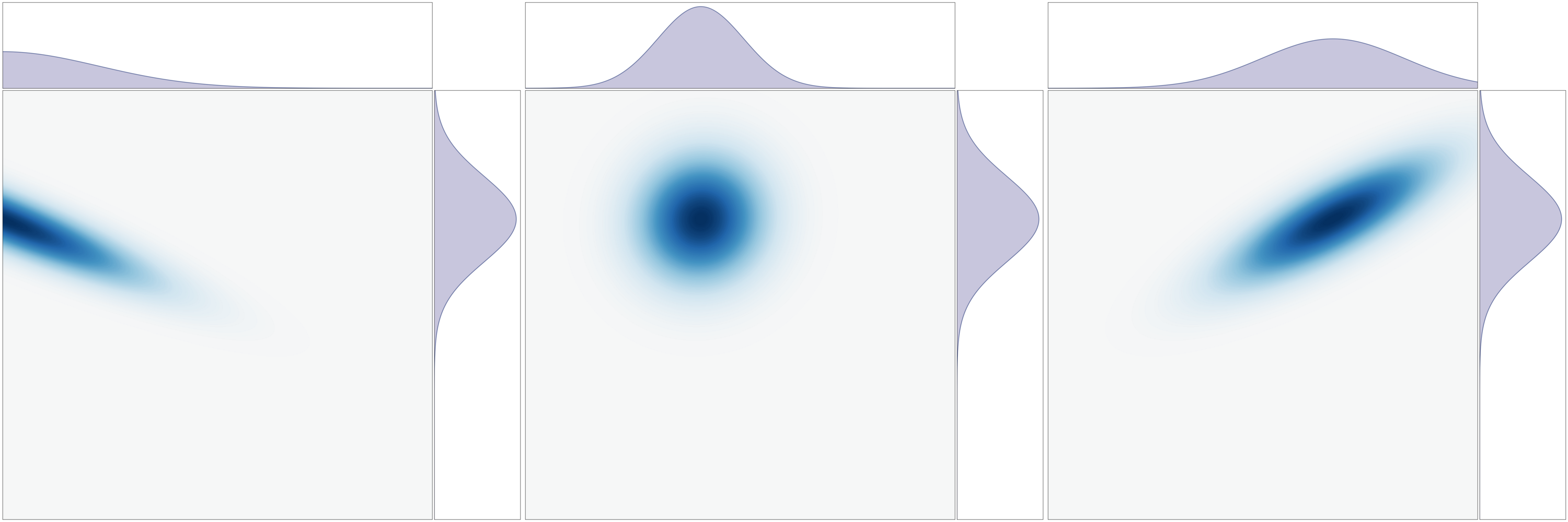
Figure 1: As time increases, a gaussian wavepacket shrinks, then spreads, on the $q$-axis marginal. Its $p$-axis marginal remains unchanged. Colors and animation online.

II.2 Negative probability flow

Refs Villanueva, 2020; Goussev, 2020 noted that for a gaussian wavepacket with positive group velocity $p_{0}/m>0$, it is often the case that there is a paradoxical “negative probability flow”. Specifically, it was found that, if we stand at a point $q_{1}>q_{0}$, and plot $Pr(q>q_{1}|t)$, the probability that the particle is found at $q>q_{1}$ at time $t$, then as time passes, that probability first decreases, before it increases, even though the wavepacket always has positive group velocity. This is immediate in the phase space picture.

Consider a gaussian wavepacket with $W(0,q,p)=\rho_{N((q_{0},p_{0}),\operatorname*{diag}(\sigma_{q}^{2},\sigma_{p}^{2}))}$, with $q_{0}<0$ and $p_{0}>0$. Geometrically, $Pr(q>q_{1}|t)$ is the integral of $W(t,q,p)$ on the region to the right of the vertical line $q=q_{1}$. Instead of shearing the gaussian, we can shear the vertical line instead. Thus, the probability is equal to the integral of $W(0,q,p)$ on the region to the right of the sheared line $q=-\frac{t}{m}p$. The sheared line rotates counterclockwise over time.

From the geometry of gaussian distributions, this integral can be visually calculated by finding the contour-ellipse of $W(0,q,p)$ that is tangent to the sheared line. At $t\to-\infty$, the sheared line is just the $q$-axis. As $t$ increases, the sheared line rotates counterclockwise, and the tangent ellipse grows, until it hits the maximal size at some extremum time $t=t_{\text{extremum}}$, at which point the tangent ellipse is equal to

$$\frac{(q-q_{0})^{2}}{\sigma_{q}^{2}}+\frac{(p-p_{0})^{2}}{\sigma_{p}^{2}}=\frac{(q_{1}-q_{0})^{2}}{\sigma_{q}^{2}}+\frac{(0-p_{0})^{2}}{\sigma_{p}^{2}}$$

It is a simple exercise to show $t_{\text{extremum}}=-\frac{mp_{0}\sigma_{q}^{2}}{(q_{1}-q_{0})\sigma_{p}^{2}}$.

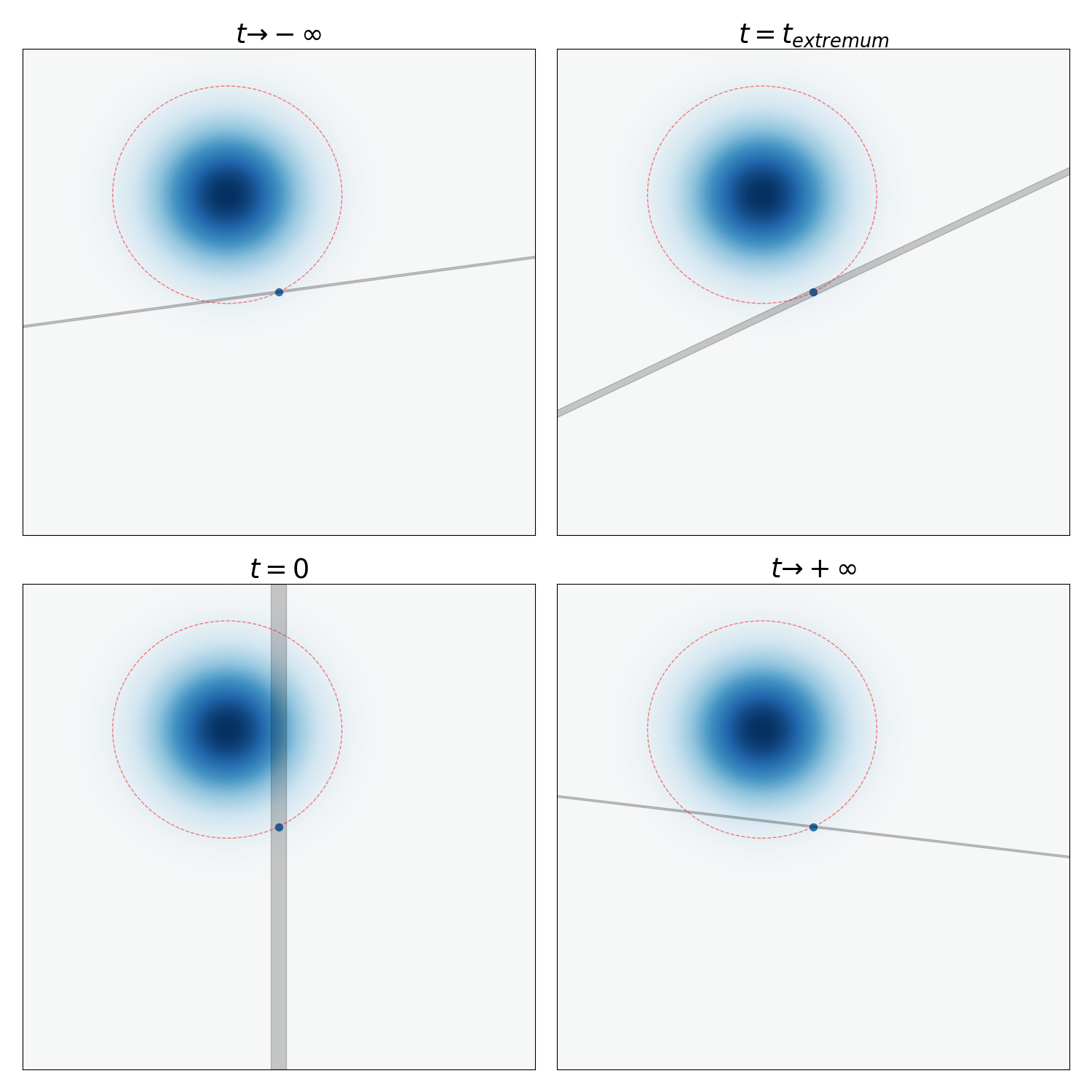
Figure 2: The negative probability flow of a gaussian wavepacket. The dashed circle is the largest possible tangent ellipse. At $t=t_{\text{extremum}}$, the sheared line is tangent to the dashed circle. Colors online.

After that, the tangent ellipse shrinks again, as the sheared line rotates towards the $q$-axis again at $t\to+\infty$. This is illustrated in Figure 2, which makes it visually clear that $Pr(q>q_{1}|t)$ decreases over the region $t\leq t_{\text{extremum}}$, and increases over the region $t\geq t_{\text{extremum}}$.

By a similar visual reasoning, if $q_{0}>0,p_{0}>0$, then $Pr(q>q_{1}|t)$ increases over the region $t\leq t_{\text{extremum}}$, and decreases over the region $t\geq t_{\text{extremum}}$. Only when $q_{0}=q_{1}$ is $Pr(q>q_{1}|t)$ strictly monotonic over all time.

II.3 Wave dispersion

As noted previously, a gaussian wave packet first shrinks, then grows, according to a precise formula proved in every introductory quantum mechanics course. We derive this formula geometrically.

Without loss of generality, consider a wavepacket with zero group velocity, centered at $q=0$, reaching minimal width $\sigma_{q}$ at $t=0$. Its Wigner function is $\rho_{N((0,0),\operatorname*{diag}(\sigma_{q}^{2},\sigma_{p}^{2}))}$, where $\sigma_{q}\sigma_{p}=\hbar/2$.

Now, consider its one-sigma ellipse $\frac{q^{2}}{\sigma_{q}^{2}}+\frac{p^{2}}{\sigma_{q}^{2}}=1$. It projects to an interval $[-\sigma_{q},+\sigma_{q}]$ on the $q$-axis, meaning that at time $t=0$, the probability of finding the particle within the interval $[-\sigma_{q},+\sigma_{q}]$ is plus-or-minus one-sigma, that is, 68.3%.

Now, at time $t$, the new one-sigma interval can be either found by shearing the Wigner function, or by shearing the $q$-intervals. As shown in Figure 3, the sheared $q$-intervals are the tangent lines to the one-sigma ellipse. The tangent line has equation $q+\frac{t}{m}p=C$ for some constant $C$. By analytic geometry, the tangent points are

$$(q,p)=\left(\frac{\sigma_{q}}{\sqrt{1+\left(\frac{\sigma_{p}t}{\sigma_{q}m}\right)^{2}}},\frac{\sigma_{p}}{\sqrt{1+\left(\frac{\sigma_{p}t}{\sigma_{q}m}\right)^{-2}}}\right)$$

and so, the projection to the $q$-axis has end points

$$\pm\sigma_{q}\sqrt{1+\left(\frac{\sigma_{p}t}{\sigma_{q}m}\right)^{2}}=\pm\sqrt{\sigma_{q}^{2}+\left(\frac{\hbar t}{2m\sigma_{q}}\right)^{2}}$$

as expected.

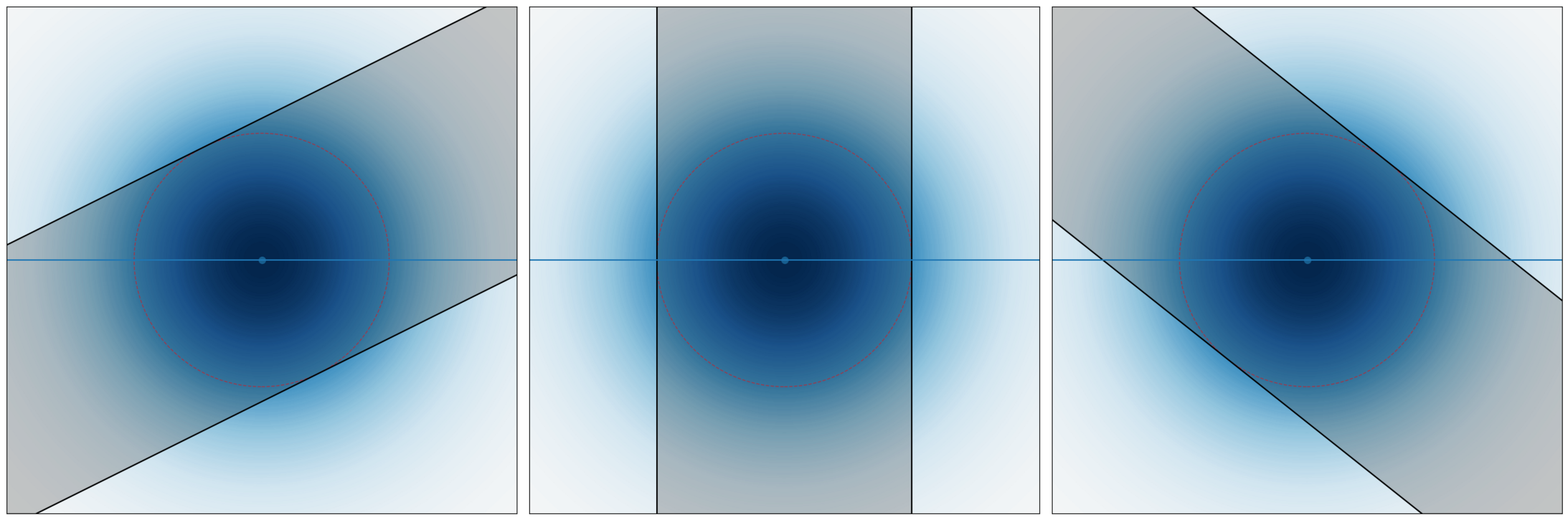
Figure 3: Gaussian wavepacket spreading. As time increases, the one-sigma circle projects to an interval on $q$-axis, which shrinks as $t\uparrow 0$, then grows as $t\uparrow\infty$. Colors and animation online.

In particular, for very large $t$, the wavepacket spreads linearly. This is in fact a generic result for arbitrary waves. Specifically, the $q$-marginal of the Wigner function at $q=q_{1}$ and time $t$ can be found by shearing a thin slice $q\in[q_{1},q_{1}+\delta q]$ back by $\frac{pt}{m}$. If $t$ is large, then this thin slice, perpendicular to the $q$-axis, is sheared to become almost perpendicular to the $p$-axis instead, which is approximately $p\in[mq_{1}/t,m(q_{1}+\delta q)/t]$. Thus, we have

$$|\psi_{q}(t,q)|^{2}\to\frac{m}{t}|\psi_{p}(0,mq_{1}/t)|^{2}$$

as $t\to+\infty$.

This is depicted for a gaussian wavepacket in Figure 4.

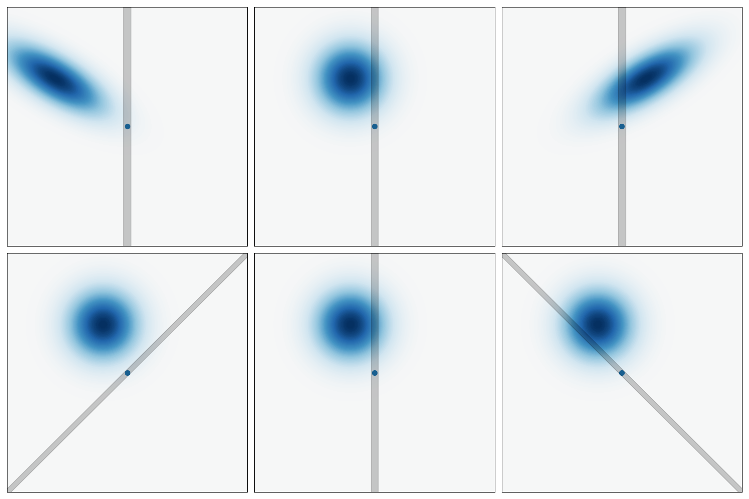
Figure 4: Shearing a gaussian Wigner function over time, then taking the marginal, is equivalent to integrating the Wigner function over vertical lines sheared in the opposite direction. Colors online.

II.4 Hermite–Gauss waves

For a simple harmonic oscillator with Hamiltonian $\frac{p^{2}}{2m}+\frac{1}{2}m\omega^{2}q^{2}$, the evolution of the Wigner function is still the same as the classical one. Thus, the Wigner function simply rotates in phase space. A standing wave for a simple harmonic oscillator, then, is some wavefunction $\psi(q)$ such that its Wigner function is rotationally symmetric.

It is proved in standard introductory quantum mechanics that such standing waves are precisely the Hermite–Gauss waves:(Griffiths and Schroeter, 2018, pp. 52–54)

$$\psi_{n}(x)=\frac{1}{\sqrt{2^{n}\,n!}}\left(\frac{m\omega}{\pi\hbar}\right)^{1/4}e^{-\frac{m\omega x^{2}}{2\hbar}}H_{n}\left(\sqrt{\frac{m\omega}{\hbar}}x\right),\qquad n=0,1,2,\ldots.$$

where $H_{n}$ are the physicist’s Hermite polynomials. Therefore, by the previous picture of how the probability density spreads, we conclude that: The Hermite–Gauss waves are the only wavefunctions whose probability density functions retain their shapes during propagation in free space.

Furthermore, the exact same argument as the previous section allows us to compute how fast the wave spreads. Though the $q$-marginal is no longer gaussian, we can still characterize its width by a single number. The precise definition does not matter, as it is only necessary to measure the shape of a Hermite–Gauss wave by a single number.

For the sake of concreteness, let $t=0$ be the point in time where the wave has minimal spread – that is, the point at which its Wigner function has contour ellipses that are not tilted, but has major axes parallel to the $q$-axis and the $p$-axis. Let $\sigma_{q}$ be the half-interquartile range. That is, between $q_{50\%}$ and $q_{75\%}$, where $q_{75\%}$ is the point such that $Pr(q\leq q_{75\%})=75\%$.

Since in the simple harmonic oscillator, the Wigner function just rotates around classically. This means that we can use the classical energy conservation formula:

$$\frac{\sigma_{p}(0)^{2}}{2m}=\frac{1}{2}m\omega^{2}\sigma_{q}(0)^{2}\implies\sigma_{p}(0)/\sigma_{q}(0)=m\omega$$

Figure 5 shows that the same geometric argument gives

$$\sigma_{q}(t)=\sigma_{q}(0)\sqrt{1+\left(\frac{\sigma_{p}(0)t}{\sigma_{q}(0)m}\right)^{2}}=\sigma_{q}(0)\sqrt{1+\left(\omega t\right)^{2}}$$

which is a surprisingly simple and elegant formula. The case of the gaussian is recovered by noting that it is the only Hermite–Gauss wave that exactly reaches the minimum allowed by the uncertainty principle: $\sigma_{q}(0)\sigma_{p}(0)=\hbar/2$, which, when combined with $\sigma_{p}(0)/\sigma_{q}(0)=m\omega$ that is satisfied by all Hermite–Gauss waves, gives us $\omega=\frac{\hbar}{2m\sigma_{q}^{2}}$, and so we recover the previous result of $\sigma_{q}(t)=\sigma_{q}(0)\sqrt{1+\left(\frac{\hbar t}{2m\sigma_{q}^{2}}\right)^{2}}$

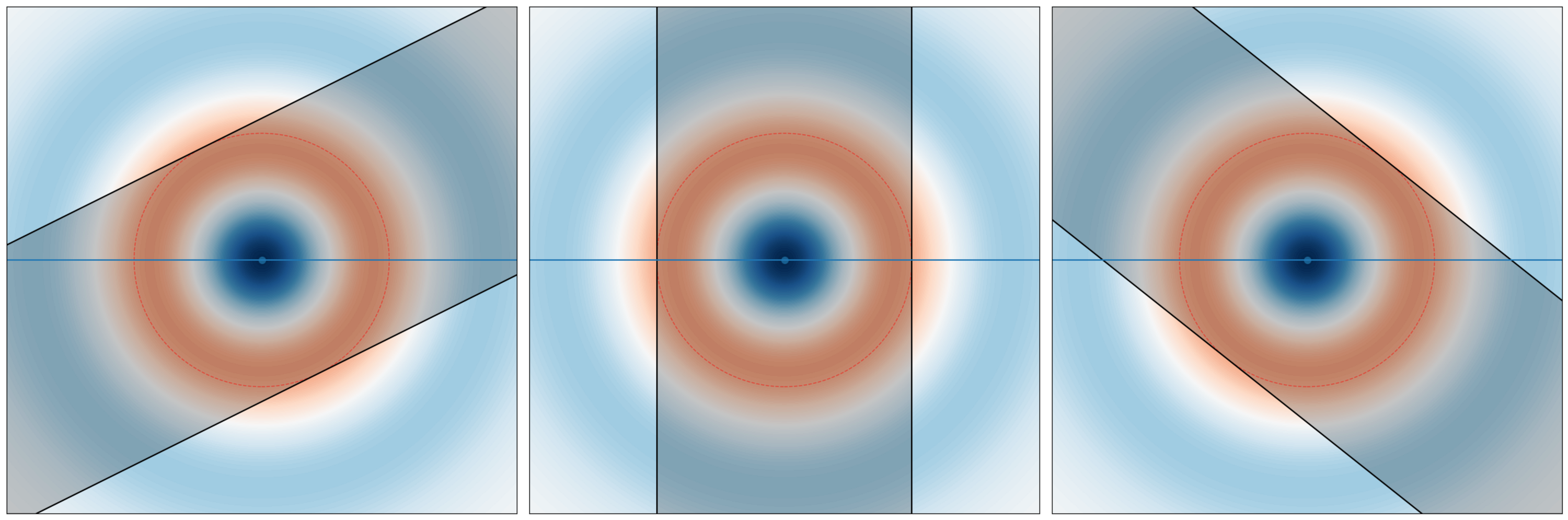
Figure 5: Spreading of the $n=2$ eigenstate of the simple harmonic oscillator. As time increases, the one-sigma circle projects to an interval on $q$-axis, which shrinks as $t\uparrow 0$, then grows as $t\uparrow\infty$. Colors and animation online.

Ref Andrews, 2008 proved these results analytically. However, as far as the author knows, this is the first time these were derived geometrically, with minimal calculus.

II.5 Square wave

As a concrete example of a wave that is not Hermite–Gauss, consider the square wave function

$$\psi(q)=\begin{cases}a^{-1/2}&\text{ if }q\in[-a/2,+a/2]\\ 0&\text{ else}\end{cases}$$

Its Wigner function is easily calculated as

$$W(0,q,p) =\frac{1}{2a\pi\hbar}\int_{|q+y/2|\leq a/2,|q-y/2|\leq a/2}dye^{-ipy/\hbar}$$

$$=\frac{1}{2a\pi\hbar}\frac{\hbar}{-ip}e^{-ipy/\hbar}\Big{|}_{\max(2q-a,-2q-a)}^{\min(2q+a,-2q+a)}$$

$$=\frac{1}{a\pi p}\sin\left(\frac{p(a-2|q|)}{\hbar}\right)$$

when $q\in[-a/2,+a/2]$. For larger values, $W=0$.

The $p$-marginal distribution is

$$\rho_{p}(p) :=\int_{\mathbb{R}}W(0,q,p)dq$$

$$=\int_{-a/2}^{+a/2}\frac{1}{a\pi p}\sin\left(\frac{p(a-2|q|)}{\hbar}\right)dq$$

$$=\frac{\hbar}{\pi ap^{2}}(1-\cos(pa/\hbar))$$

The Wigner function and its $p$-marginal are shown in Figure 6.

Let $f(t):=\frac{1-\cos t}{\pi t^{2}}=\left(\frac{\operatorname{sinc}(t/2)}{\sqrt{2\pi}}\right)^{2}$, then $\rho_{p}(p)=\frac{a}{\hbar}f(\frac{a}{\hbar}p)$. Thus, the $p$-marginal distribution always has the same shape no matter what $a$ is.

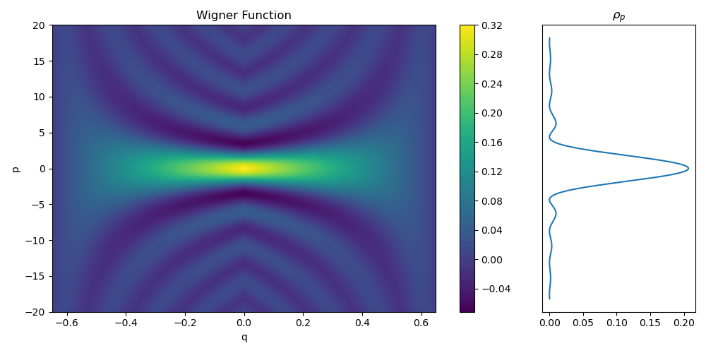
Figure 6: The Wigner function of the square wave and its $p$-marginal distribution. $a=1.3,\hbar=1$. Colors online.

Because at $t=0$, the Wigner function is zero outside of $q\in[-a/2,+a/2]$, at large $t$, the probability that the particle is found at $[q,q+\delta q]$ is the integral of $W(0,\cdot,\cdot)$ over a the thin line passing $[q,q+\delta q]$ at slope $-m/t$. Thus, we have

$$\int_{\mathbb{R}}W(t,q,p)dp \approx\frac{m}{t}\int_{-a/2}^{+a/2}W(0,q,p)dq$$

$$=\frac{m}{t}\rho_{p}(qm/t)=\frac{\hbar t}{\pi maq^{2}}\left(1-\cos\left(\frac{ma}{\hbar t}q\right)\right)$$

$$=\frac{am}{\hbar t}f\left(\frac{am}{\hbar t}q\right)$$

In particular, the higher-order waves are not disspated away, and so the square wave never converges to a gaussian wavepacket. In fact, it always converges to the same shape of $f$. This is directly against the claim of Ref Mita, 2007, as previously pointed out by Ref Andrews, 2008.

By the symmetry of the Wigner function in $q$ and $p$, we have the following result: If the wavefunction satisfies $\psi(q)=\sqrt{\frac{b}{\hbar}}\frac{\operatorname{sinc}(bq/2\hbar)}{\sqrt{2\pi}}$ at $t=0$, then at large $t$, the wavefunction converges to a square wave on the interval $[-bt/2m,+bt/2m]$ with height $\sqrt{\frac{m}{bt}}$.

II.6 Generic wavepacket

In general, the shape of the wave of any normalizable wave function $\psi_{q}(q)$, propagating in free space, would, after a long time, converge to a translation-and-dilation of its $p$-marginal distribution $\psi_{q}(q)$, multiplied by a phase factor $e^{iS(t,q)}$. Since the $q$-marginal distribution can be arbitrary, the same is true for the $p$-marginal distribution. In particular, we have the following theorem, which is immediate from the geometric intuition.

Theorem 1.

If $\rho$ is a smooth probability density function on $\mathbb{R}$, then there exists a wavefunction $\psi$ propagating in free space, such that for all large enough $t$,

$$|\psi(t,q)|^{2}\to\frac{m}{t}\rho(mq/t)$$

Proof.

Such $\psi(0,q)$ can be found by taking the Wigner function of $\sqrt{\rho(p)}e^{iS(p)}$ for an arbitrary smooth function $S$, rotating by 90 degrees in the phase plane, then taking the inverse Wigner transform.

∎

Previously, we showed that for almost any gaussian wavepacket, $Pr(q>q_{1}|t)$, i.e. the probability of finding the particle to the right of some point $q_{1}$ at time $t$, would first increase then decrease, or first decrease then increase. In fact, this is true for almost any Wigner function, period. The Wigner function does not even need to be pure. It can be the Wigner function of a mixed state, and this would still be true.

Theorem 2.

For almost any mixed state of a particle propagating in free space, and almost any $q_{1}$, the function $t\mapsto Pr(q>q_{1}|t)$ is not monotonic.

Proof.

Fix some Wigner function $W$. Define $f(\theta)$ to be the integral of $W$ to the right of the line passing $(q_{1},0)$, making an angle $\theta$ with the $q$-axis. Then we have $f(0)=1-f(\pi)$, and in general, $f(\theta)=1-f(\pi+\theta)$. Thus, if $f$ reaches a global minimum at $\theta$, then it reaches a global maximum at $f(\theta+\pi)$. In particular, if $f(0)$ is neither the global minimum nor the global maximum, then $f(\theta)$ must reach either the global minimum or the global maximum at some $\theta\in(0,\pi)$. Therefore, $f$ is not monotonic as $\theta$ rotates from $0$ to $\pi$.

∎

We can think of this as a “maximally non-dissipation” result. Unlike the heat equation, where all high-frequency fluctuations decay away, leaving behind just a single low-frequency gaussian mode, the Schrödinger equation results in a wave propagation that has no dissipation, but preserves the shape of $|\psi_{p}(0)|^{2}$ for all large times. This is unsurprising, as it is a common folklore that quantum mechanical wavefunctions, like classical waves, do not dissipate.

III Conclusion

The dynamics of wavefunctions in free space, while often covered in introductory courses using analytical tools, can be somewhat unintuitive. Switching to the phase-space formulation of quantum mechanics, while not traditionally done, offers a way of visualizing these dynamics using the Wigner function. The spreading, shearing, the so-called “negative probability flow” of wavefunctions, and the long-time asymptotic dispersion of waves, become visually intuitive. Educators may find it pedagogically useful to visualize the Wigner function, alongside the more traditional analytical derivations, in an introductory quantum mechanics course. The material is perhaps even teachable to gifted high-school students.

Data Availability Statement

The plotting code and animations are available both as supplementary material available at the official website American Journal of Physics and at the author’s personal website.

References

- Case (2008) W. B. Case, “Wigner functions and Weyl transforms for pedestrians,” American Journal of Physics 76, 937–946 (2008).
- Curtright, Fairlie, and Zachos (2014) T. Curtright, D. Fairlie, and C. Zachos, A Concise Treatise on Quantum Mechanics in Phase Space (World Scientific, New Jersey, 2014).
- Berry and Balazs (1979) M. V. Berry and N. L. Balazs, “Nonspreading wave packets,” American Journal of Physics 47, 264–267 (1979).
- Villanueva (2020) A. A. D. Villanueva, “The negative flow of probability,” American Journal of Physics 88, 325–333 (2020).
- Goussev (2020) A. Goussev, “Comment on “The negative flow of probability” [Am. J. Phys. 88, 325–333 (2020)],” American Journal of Physics 88, 1023–1028 (2020).
- Note (1) Even this minimal amount of analytic geometry can be eliminated, resulting an almost purely geometric argument. First, stretch the -axis by and -axis by , turning the one-sigmal circle to a unit circle. This changes the shear line’s slope angle to satisfying . Then, the required tangent point is . Now undo the stretching to find the tangent point in the original, un-stretched phase space.
- Griffiths and Schroeter (2018) D. J. Griffiths and D. F. Schroeter, Introduction to Quantum Mechanics, 3rd ed. (Cambridge University Press, Cambridge, United Kingdom, 2018).
- Andrews (2008) M. Andrews, “The evolution of free wave packets,” American Journal of Physics 76, 1102–1107 (2008).
- Mita (2007) K. Mita, “Dispersion of non-Gaussian free particle wave packets,” American Journal of Physics 75, 950–953 (2007).
- Nebula (2024) C. Nebula, “English: Wigner quasiprobability distribution of cat state, n = 10, a = 10.” (2024).
- Mita (2021) K. Mita, “Schrödinger’s equation as a diffusion equation,” American Journal of Physics 89, 500–510 (2021).