The Parameterized Complexity of
Extending Stack Layouts

Abstract

An $\ell$-page stack layout (also known as an $\ell$-page book embedding) of a graph is a linear order of the vertex set together with a partition of the edge set into $\ell$ stacks (or pages), such that the endpoints of no two edges on the same stack alternate. We study the problem of extending a given partial $\ell$-page stack layout into a complete one, which can be seen as a natural generalization of the classical -hard problem of computing a stack layout of an input graph from scratch. Given the inherent intractability of the problem, we focus on identifying tractable fragments through the refined lens of parameterized complexity analysis. Our results paint a detailed and surprisingly rich complexity-theoretic landscape of the problem which includes the identification of para-hard, [1]-hard and -tractable, as well as fixed-parameter tractable fragments of stack layout extension via a natural sequence of parameterizations.

1 Introduction

An $\ell$-page stack layout (or $\ell$-page book embedding) of a graph $G$ consists, combinatorially speaking, of (i) a linear order $\prec$ of its vertex set $V(G)$ and (ii) a partition $\sigma$ of its edge set $E(G)$ into $\ell\geq 1$ (stack-)pages such that for no two edges (with distinct endpoints) $uv$ and $wx$ with $u\prec v$ and $w\prec x$ that are assigned to the same page their endpoints alternate in $\prec$, i.e., we have $u\prec w\prec v\prec x$. When drawing a stack layout, the vertices are placed on a line called the spine in the order given by $\prec$ and the edges of each page are drawn as pairwise non-crossing arcs in a separate half-plane bounded by the spine, see Figure 1a.

Figure 1: (a) A graph $H$ and a two-page stack layout of it. In (b), the graph $H$ and its two-page stack layout are extended by the new vertices and edges marked in blue.

Stack layouts are a classic and well-studied topic in graph drawing and graph theory [6, 29, 12]. They have immediate applications in graph visualization [37, 4, 24] as well as in bioinformatics, VLSI design, and parallel computing [14, 26]; see also the overview by Dujmović and Wood [19].

The minimum number $\ell$ such that a given graph $G$ admits an $\ell$-page stack layout is known as the stack number, page number, or book thickness of $G$. While the graphs with stack number $\ell=1$ are the outerplanar graphs, which can be recognized in linear time, the problem of computing the stack number is -complete in general. Indeed, the class of graphs with stack number $\ell\leq 2$ are precisely the subhamiltonian graphs (i.e., the subgraphs of planar Hamiltonian graphs) and recognizing them is -complete [6, 14, 38]. Computing the stack number is known to also remain -complete if the vertex order is provided as part of the input and $\ell=4$ [35], and overcoming the intractability of these problems has been the target of several recent works in the field [11, 10, 28, 23]. Many other results on stack layouts are known—for instance, every planar graph has a $4$-page stack layout and this bound is tight [39, 5]. For a comprehensive list of known upper and lower bounds for the stack number of different graph classes, we refer to the collection by Pupyrev [32].

In this paper, we take a new perspective on stack layouts, namely the perspective of drawing extensions. In drawing extension problems, the input consists of a graph $G$ together with a partial drawing of $G$, i.e., a drawing of a subgraph $H$ of $G$. The task is to insert the vertices and edges of $G$ which are missing in $H$ in such a way that a desired property of the drawing is maintained; see Figure 1b for an example. Such drawing extension problems occur, e.g., when visualizing dynamic graphs in a streaming setting, where additional vertices and edges arrive over time and need to be inserted into the existing partial drawing. Drawing extension problems have been investigated for many types of drawings in recent years—including planar drawings [1, 27, 31, 30], upward planar drawings [16], level planar drawings [13], $1$-planar drawings [20, 21], and planar orthogonal drawings [3, 2, 9]—but until now, essentially nothing was known about the extension of stack layouts/book embeddings.

Since it is -complete to determine whether a graph admits an $\ell$-page stack layout (even when $\ell$ is a small fixed integer), the extension problem for $\ell$-page stack layouts is -complete as well—after all, setting $H$ to be empty in the latter problem fully captures the former one. In fact, the extension setting can seemlessly also capture the previously studied -complete problem of computing an $\ell$-stack layout with a prescribed vertex order [14, 35, 36, 11, 10]; indeed, this corresponds to the special case where $V(H)=V(G)$ and $E(H)=\emptyset$. Given the intractability of extending $\ell$-page stack layouts in the classical complexity setting, we focus on identifying tractable fragments of the problem through the more refined lens of parameterized complexity analysis [18, 15], which considers both the input size of the graph and some additional parameter $k$ of the instance.

Figure 2: The complexity landscape of Stack Layout Extension. VEDD denotes the vertex+edge deletion distance, $\omega$ denotes the page width of the $\ell$-page stack layout of $H$, and $\kappa=\left|V(G)\setminus V(H)\right|+\left|E(G)\setminus E(H)\right|$. Boxes outlined in bold represent new results that we show in the linked theorems and corollaries. The only result that is not depicted is Theorem 3.2.

Contributions.

A natural parameter in any drawing extension problem is the size of the missing part of the graph, i.e., the missing number of vertices and/or edges. We start our investigation by showing that the Stack Layout Extension problem (SLE) for instances without any missing vertices, i.e., $V(G)=V(H)$, is fixed-parameter tractable when parameterized by the number of missing edges $|E(G)\setminus E(H)|$ (Section 3).

The above result, however, only applies in the highly restrictive setting where no vertices are missing—generally, we would like to solve instances with missing vertices as well as edges. A parameterization that has been successfully used in this setting is the vertex+edge deletion distance, i.e., the number of vertex and edge deletion operations required to obtain $H$ from $G$. But while this parameter has yielded parameterized algorithms when extending, e.g., 1-planar drawings [20, 21] and orthogonal planar drawings [9], we rule out any analogous result for SLE by establishing its -completeness even if $H$ can be obtained from $G$ by deleting only two vertices (Section 4). This means that more “restrictive” parameterizations are necessary to achieve tractability for the problem of extending $\ell$-page stack layouts.

Since the missing vertices in our hardness reduction have a high degree, we then consider parameterizations by the combined number of missing vertices and edges $\kappa=\left|V(G)\setminus V(H)\right|+\left|E(G)\setminus E(H)\right|$. We show that SLE belongs to the class  when parameterized by $\kappa$ (Section 5) while being [1]-hard (Section 6), which rules out the existence of a fixed-parameter tractable algorithm under standard complexity assumptions. The latter result holds even if we additionally bound the page width $\omega$ of the stack layout of $H$, which measures the maximum number of edges that are crossed on a single page by a line perpendicular to the spine [14]. On our quest towards a fixed-parameter tractable fragment of the problem, we thus need to include another restriction, namely the number $\ell$ of pages of the stack layout. So finally, when parameterizing SLE by the combined parameter $\kappa+\omega+\ell$, we show that it becomes fixed parameter tractable (Section 7). Our results are summarized in Figure 2.

2 Preliminaries

We assume the reader to be familiar with standard graph terminology [17]. Throughout this paper, we assume standard graph representations, e.g., as double-linked adjacency list, that allow for efficient graph modifications. For two integers $p\leq q$ we denote with $[p,q]$ the set $\{p,p+1,\ldots,q\}$ and use $[p]_{0}$ and $[p]$ as abbreviations for $[0,p]$ and $[1,p]$, respectively. Let $G$ be a graph that is, unless stated otherwise, simple and undirected, with vertex set $V(G)$ and edge set $E(G)$. For $X\subseteq V(G)$, we denote by $G[X]$ the subgraph of $G$ induced on $X$.

Stack Layouts.

For an integer $\ell\geq 1$, an $\ell$-page stack layout of $G$ is a tuple $\langle\prec_{G},\sigma_{G}\rangle$ where $\prec_{G}$ is a linear order of $V(G)$ and $\sigma_{G}\colon E(G)\to[\ell]$ is a function that assigns each edge to a page $p\in[\ell]$ such that for each pair of edges $u_{1}v_{1}$ and $u_{2}v_{2}$ with $\sigma(e_{1})=\sigma(e_{2})$ it does not hold $u_{1}\prec u_{2}\prec v_{1}\prec v_{2}$. For the remainder of the paper, we write $\prec$ and $\sigma$ if the graph $G$ is clear from context. We call $\prec$ the spine (order) and $\sigma$ the page assignment. Observe that we can interpret a stack layout as a drawing of $G$ on different planar half-planes, one per page $p\in[\ell]$, each of which is bounded by the straight-line spine delimiting all half-planes. One fundamental property of a stack layout is its page width—denoted as $\omega(\langle\prec,\sigma\rangle)$ or simply $\omega$ if $\langle\prec,\sigma\rangle$ is clear from context—which is the maximum number of edges that are crossed on a single page by a line perpendicular to the spine [14]. The properties of stack layouts with small page width have been studied, e.g., by Stöhr [34, 33].

We say that two vertices $u$ and $v$ are consecutive on the spine if they occur consecutively in $\prec$. A vertex $u\in V(G)$ sees a vertex $v\in V(G)$ on a page $p\in[\ell]$ if there does not exist an edge $e=xy\in E(G)$ with $\sigma(e)=p$ and $x\prec u\prec y\prec v$ or $u\prec x\prec v\prec y$. Note that if $u$ sees $v$, then $v$ also sees $u$. For two vertices $u$ and $v$ which are consecutive in $\prec$, we refer to the segment on the spine between $u$ and $v$ as the interval between $u$ and $v$, denoted as $[u,v]$.

Problem Statement.

Let $H\subseteq G$ be a subgraph of a graph $G$. We say that $\langle\prec_{G},\sigma_{G}\rangle$ is an extension of $\langle\prec_{H},\sigma_{H}\rangle$ if $\sigma_{H}\subseteq\sigma_{G}$ and $\prec_{H}\subseteq\prec_{G}$. We now formalize our problem of interest:

Stack Layout Extension (SLE) Given Integer $\ell\geq 1$, graph $G$, subgraph $H$ of $G$, and $\ell$-page stack layout $\langle\prec_{H},\sigma_{H}\rangle$. Question Does there exist an $\ell$-page stack layout $\langle\prec_{G},\sigma_{G}\rangle$ of $G$ that extends $\langle\prec_{H},\sigma_{H}\rangle$?

We remark that while SLE is defined as a decision problem for complexity-theoretic reasons, every algorithm presented in this article is constructive and can be trivially adapted to also output a layout $\langle\prec_{G},\sigma_{G}\rangle$ as a witness (also called a solution) for positive instances. For an instance $\mathcal{I}$ of SLE, we use $\left|\mathcal{I}\right|$ as shorthand for $|V(G)|+|E(G)|+\ell$.

In line with the terminology previously used for drawing extension problems [20], we refer to the vertices and edges in $V(H)\cup E(H)$ as old and call all other vertices and edges of $G$ new. Let $V_{\text{add}}$ and $E_{\text{add}}$ denote the sets of all new vertices and edges, respectively, and set $n_{\text{add}}{}\coloneqq\left|V_{\text{add}}{}\right|$ and $m_{\text{add}}{}\coloneqq\left|E_{\text{add}}{}\right|$. Furthermore, we denote with $E_{\text{add}}^{H}$ the set of new edges incident to two old vertices, i.e., $E_{\text{add}}^{H}{}\coloneqq\{e=uv\in E_{\text{add}}{}\mid u,v\in V(H)\}$. We consider the parameterized complexity of our extension problem by measuring how “incomplete” the provided partial solution is using the following natural parameters that have also been used in this setting before [20, 21, 22, 8, 7]: the vertex+edge deletion distance, which is $n_{\text{add}}+\left|E_{\text{add}}^{H}\right|$, and the total number of missing vertices and edges, i.e., $n_{\text{add}}+m_{\text{add}}$.

3 SLE With Only Missing Edges is

We begin our investigation by first analyzing the special case where $V(G)=V(H)$, i.e., when only edges are missing from $H$. We recall that the problem remains -complete even in this setting, as it generalizes the problem of computing the stack number of a graph with a prescribed vertex order [14, 35, 36, 11, 10]. Furthermore, both of the aforementioned measures of the incompleteness of $\langle\prec_{H},\sigma_{H}\rangle$ are the same and equal $m_{\text{add}}=\left|E_{\text{add}}^{H}\right|$. As a “warm-up” result, we show that in this setting SLE is fixed-parameter tractable parameterized by $m_{\text{add}}$.

Towards this, consider the set $S(e)\subseteq[\ell]$ of pages on which we could place a new edge $e$ without introducing a crossing with edges from $H$; formally, $p\in S(e)$ if and only if $\langle\prec_{H},\sigma_{H}\cup{(e,p)}\rangle$ is an $\ell$-page stack layout of $H\cup\{e\}$. Intuitively, if $\left|S(e)\right|$ is large enough, then we are always able to find a “free” page to place $e$ independent of the placement of the remaining new edges. Formally, one can easily show:

Lemma 3.1.

Let $\mathcal{I}=\left(\ell,G,H,\langle\prec,\sigma\rangle\right)$ be an instance of SLE with $V_{\text{add}}{}=\emptyset$ that contains an edge $e\in E_{\text{add}}{}$ with $\left|S(e)\right|\geq m_{\text{add}}{}$. The instance $\mathcal{I}^{\prime}=\left(\ell,H,G^{\prime},\langle\prec,\sigma\rangle\right)$ with $G^{\prime}=G\setminus\{e\}$ is a positive instance if and only if $\mathcal{I}$ is a positive instance.

plemmaOnlyEdgesRemoveEasyEdges First, note that removing an edge from $G$ and adapting the page assignment $\sigma$ accordingly does not invalidate an existing solution $\langle\prec,\sigma\rangle$ to SLE for $\mathcal{I}$. Hence, the “($\boldsymbol{\Leftarrow}$)-direction” holds trivially, and we focus on the “($\boldsymbol{\Rightarrow}$)-direction”.

*($\boldsymbol{\Rightarrow}$) Let $\mathcal{I}^{\prime}$ be a positive instance of SLE with the solution $\langle\prec,\sigma\rangle$. By our selection of $e$, there exists a page $p\in S(e)$ such that we have for every edge $e^{\prime}\in E_{\text{add}}{}$ with $e^{\prime}\neq e$ that $\sigma(e^{\prime})\neq p$ holds. We take $\langle\prec,\sigma\rangle$ and extend $\sigma$ by the page assignment $(e,p)$ to obtain $\langle\prec_{G},\sigma_{G}\rangle$. By the definition of $S(\cdot)$, this cannot introduce a crossing with edges from $H$ and by our selection of $p$, no crossings with other edges from $E_{\text{add}}{}$ are possible either. Hence, $\langle\prec_{G},\sigma_{G}\rangle$ is a valid stack layout of $G$ that extends $\langle\prec_{H},\sigma_{H}\rangle$ as we did not alter $\langle\prec,\sigma\rangle$ except extending the page assignment. Thus, it witnesses that $\mathcal{I}$ is a positive instance of SLE. With Lemma 3.1 in hand, we can establish the desired result:

Theorem 3.2.

Let $\mathcal{I}=\left(\ell,G,H,\langle\prec,\sigma\rangle\right)$ be an instance of SLE with $V_{\text{add}}=\emptyset$. We can find an $\ell$-page stack layout of $G$ that extends $\langle\prec,\sigma\rangle$ or report that none exists in $\mathcal{O}(m_{\text{add}}{}^{m_{\text{add}}{}}\cdot\left|\mathcal{I}{}\right|)$ time.

We compute for a single edge $e\in E_{\text{add}}{}$ the set $S(e)$ in linear time by checking with which of the old edges $e$ would cross. If $S(e)\geq m_{\text{add}}{}$, then following Lemma 3.1, we remove $e$ from $G$. Overall, this takes $\mathcal{O}(m_{\text{add}}{}\cdot\left|\mathcal{I}{}\right|)$ time and results in a graph $G^{\prime}$ with $H\subseteq G^{\prime}\subseteq G$. Furthermore, each remaining new edge $e^{\prime}\in E(G^{\prime})\setminus E(H)$ can be put in fewer than $m_{\text{add}}{}$ different pages. Hence, we can brute-force over all the at most $\mathcal{O}(m_{\text{add}}{}^{m_{\text{add}}{}})$ page assignments $\sigma^{\prime}$ that extend $\sigma_{H}$ for all edges in $E(G^{\prime})\setminus E(H)$, and for each such assignment we check in linear time whether no pair of edges $e^{\prime},e^{\prime\prime}\in E(G^{\prime})\setminus E(H)$ cross each other. ptheoremOnlyEdgesFPT We compute for a single edge $e\in E_{\text{add}}{}$ the set $S(e)$ in linear time by checking with which of the old edges $e$ would cross. If $S(e)\geq m_{\text{add}}{}$, then we remove $e$ from $G$. Overall, this takes $\mathcal{O}(m_{\text{add}}{}\cdot\left|\mathcal{I}{}\right|)$ time and results in a graph $G^{\prime}$ with $H\subseteq G^{\prime}\subseteq G$. Furthermore, each edge $e^{\prime}\in E(G^{\prime})\setminus E(H)$ can be put in fewer than $m_{\text{add}}{}$ different pages. Hence, we can brute force the possible page assignments for each new edge $e^{\prime}$. Each of the resulting $\mathcal{O}(m_{\text{add}}{}^{m_{\text{add}}{}})$ different $\ell$-page stack layouts $\langle\prec,\sigma\rangle$ is by construction an extension of $\langle\prec_{H},\sigma_{H}\rangle$. Creating $\langle\prec,\sigma\rangle$ can be done by copying $\langle\prec_{H},\sigma_{H}\rangle$ and then augmenting it with $\mathcal{O}(m_{\text{add}}{})$ new edges. This amounts to $\mathcal{O}(\left|\mathcal{I}{}\right|)$ time. For each created $\ell$-page stack layout, we can check in linear time whether it is crossing free. Note that by our pre-processing step, no new edge can cross an old edge, and thus it suffices to check whether no pair of edges $e^{\prime},e^{\prime\prime}\in E(G^{\prime})\setminus E(H)$ cross each other. If there exists a crossing free layout, then applying Lemma 3.1 iteratively tells us that we can extend it to a solution $\langle\prec_{G},\sigma_{G}\rangle$ for $\mathcal{I}$. If none of them is crossing free, we conclude by applying (iteratively) Lemma 3.1 that $\mathcal{I}$ does not admit the desired $\ell$-page stack layout. Combining all, the overall running time is $\mathcal{O}(m_{\text{add}}{}^{m_{\text{add}}{}}\cdot\left|\mathcal{I}{}\right|)$.

4 SLE With Two Missing Vertices is -complete

Adding only edges to a given linear layout is arguably quite restrictive. Therefore, we now lift this restriction and consider SLE in its full generality, i.e., also allow adding vertices. Somewhat surprisingly, as our first result in the general setting we show that SLE is -complete even if the task is to merely add two vertices, i.e., for $n_{\text{add}}{}=2$ and $E_{\text{add}}^{H}{}=\emptyset$. This rules out not only fixed-parameter but also  tractability when parameterizing by the vertex+edge deletion distance, and represents—to the best of our knowledge—the first example of a drawing extension problem with this behavior.

To establish the result, we devise a reduction from 3-Sat [25]. sectionParaNPIntuitionLet $\varphi=(\mathcal{X},\mathcal{C})$ be an instance of 3-Sat consisting of $N$ variables $\mathcal{X}=\{x_{1},\ldots,x_{N}\}$ and $M$ clauses $\mathcal{C}=\{c_{1},\ldots,c_{M}\}$, each consisting of three different and pairwise non-complementary literals. Intuitively, the reduction constructs an instance $\mathcal{I}{}=\left(\ell,G,H,\langle\prec,\sigma\rangle\right){}$ of SLE which represents each variable $x_{i}$ and each clause $c_{j}$ of $\varphi$, respectively, by a corresponding vertex in $H$. The linear order $\prec_{H}$ has the form $x_{1}\prec x_{2}\prec\ldots\prec x_{N}\prec c_{1}\prec\ldots\prec c_{M}$; see Figure 3. Furthermore, $\mathcal{I}$ contains two new vertices $s$ and $v$. The vertex $s$ is adjacent to all variable-vertices and the construction will ensure that the page assignment for its incident edges represents, i.e., selects, a truth assignment $\Gamma$ for $\varphi$. The vertex $v$ is adjacent to all clause-vertices, and its purpose is to verify that the truth assignment satisfies all clauses. For the following high-level description of how this is achieved, we assume $s\prec v\prec x_{1}$ and will ensure later that every solution $\langle\prec,\sigma\rangle$ of $\mathcal{I}$ has this property.

To each variable $x_{i}$, we associate two pages $p_{i}$ and $p_{\lnot i}$ corresponding to its possible truth states. We ensure that $s$ can see each variable-vertex only on its associated pages using edges incident to dummy vertices $d_{q}$ with $q\in[N+M+1]$. These dummy vertices are distributed as in Figure 3. Hence, a page assignment for the edges incident to $s$ induces a truth assignment. Similar edges also ensure that $v$ can see a clause-vertex $c_{j}$ only on the pages that are associated to the negation of the literals the clause $c_{j}$ is composed of, see Figure 3. We defer the full construction to Section 4.1. If an induced truth assignment does not satisfy a clause $c_{j}$, then it must use the pages associated to the negated literals of $c_{j}$. Thus, the new edge $vc_{j}$ will cross another edge no matter which page we use, see also Figure 4. However, if a clause $c_{j}$ is satisfied, we can find a page for the edge $vc_{j}$ that does not introduce a crossing: the page associated to the negation of the literal that satisfies $c_{j}$. Consequently, if $\varphi$ is satisfiable, then there exists an extension $\langle\prec_{G},\sigma_{G}\rangle$. Similarly, the page assignment of an extension $\langle\prec_{G},\sigma_{G}\rangle$ induces a truth assignment $\Gamma$ that satisfies $\varphi$.

Finally, recall that our approach hinges on some way to restrict the new vertices $s$ and $v$ to be placed within a certain range, i.e., before $x_{1}$. We realize this using the fixation gadget that we describe in Section 4.2. We also reuse this gadget in the reduction from Section 6. In Section 4.3, we show how this can be build into our reduction to prove Theorem 4.2.

The graph $H$ that we construct will have multi-edges to facilitate the presentation of the reduction. The procedure for removing multi-edges is detailed in Appendix A. sectionParaNPBaseLayout

Figure 3: Parts of the spine order $\prec_{H}$. Green vertices represent variables, blue vertices clauses, and red vertices the dummy vertices. Furthermore, we visualize some edges in $H$ that are created for the variable-vertices (left) and clause-vertices (middle and right). If an edge is created due to the (non-)existence of a literal in the clause $c_{1}$, $c_{2}$, or $c_{M}$ it is indicated via a blue arc.

4.1 Encoding the Variables and Clauses: The Base Layout

For each variable $x_{i}$ and each clause $c_{j}$ in $\varphi$ we introduce a vertex in $H$. In the following, we use the same symbol to address an element of $\varphi$ and its representation in $H$. Let us first fix the spine order $\prec_{H}$. For every $i\in[N-1]$ and $j\in[M-1]$, we set $x_{i}\prec x_{i+1}$ and $c_{j}\prec c_{j+1}$. Furthermore, we order the variables before the clauses on the spine, i.e., we set $x_{N}\prec c_{1}$. Next, we add $N+M+1$ dummy vertices $d_{q}$ to $H$ and distribute them on the spine. More concretely, we set $d_{i}\prec x_{i}\prec d_{i+1}$ and $d_{N+j}\prec c_{j}\prec d_{N+j+1}$ for every $i\in[N]$ and $j\in[M]$. By taking the transitive closure of the above order, we obtain the following linear order, which we also visualize in Figure 3.

$$d_{1}\prec x_{1}\prec d_{2}\prec x_{2}\prec\ldots\prec x_{N}\prec d_{N+1}\prec c_{1}\prec\ldots\prec c_{M}\prec d_{N+M+1}$$

We now turn our attention to the page assignment $\sigma_{H}$ and create for each variable $x_{i}\in\mathcal{X}$ the two pages $p_{i}$ and $p_{\lnot i}$. Intuitively, the assignment of an edge incident to $x_{i}$ to either of these two pages will determine whether $x_{i}$ is true or false. For each $i,j\in[N]$ with $i\neq j$, we create the edges $e(x_{i},p_{j})=d_{i}d_{i+1}$ and $e(x_{i},p_{\lnot j})=d_{i}d_{i+1}$ in $H$. We assign the edge $e(x_{i},p_{j})$ to the page $p_{j}$ and the edge $e(x_{i},p_{\lnot j})$ to $p_{\lnot j}$, i.e., we have $\sigma(e(x_{i},p_{j}))=p_{j}$ and $\sigma(e(x_{i},p_{\lnot j}))=p_{\lnot j}$. Figure 3 (left) visualizes this. Note that this introduces multi-edges in $H$, but recall that we resolve them in Appendix A. In particular, we will address these multi-edges in Section A.2. Next, we consider each combination of a clause $c_{j}\in\mathcal{C}$ and a variable $x_{i}\in\mathcal{X}$. If $x_{i}$ does not appear in $c_{j}$, we create the edges $e(c_{j},p_{i})=d_{N+j}d_{N+j+1}$ and $e(c_{j},p_{\lnot i})=d_{N+j}d_{N+j+1}$. Similar to before, we set $\sigma(e(c_{j},p_{i}))=p_{i}$ and $\sigma(e(c_{j},p_{\lnot i}))=p_{\lnot i}$. If $x_{i}$ appears in $c_{j}$ without negation, we create the edge $e(c_{j},p_{i})=d_{N+j}d_{N+j+1}$ and set $\sigma(e(c_{j},p_{i}))=p_{i}$. Symmetrically, if $x_{i}$ appears negated in $c_{j}$, we create the edge $e(c_{j},p_{\lnot i})=d_{N+j}d_{N+j+1}$ and set $\sigma(e(c_{j},p_{\lnot i}))=p_{\lnot i}$. We visualize this page assignment in Figure 3 (middle and right).

This completes the base layout of our reduction. However, we have only defined parts of $H$ and its stack layout $\langle\prec,\sigma\rangle$ and complete the construction in Section 4.3. Next, we introduce two new vertices $s$ and $v$ in $G$. The vertex $s$ is adjacent to each $x_{i}\in\mathcal{X}$ and the vertex $v$ is adjacent to each $c_{j}\in\mathcal{C}$. Let us assume for the moment that in every extension $\langle\prec_{G},\sigma_{G}\rangle$ of $\langle\prec_{H},\sigma_{H}\rangle$ we have $s\prec v\prec d_{1}$. Then, the vertex $s$ can “see” each $x_{i}\in\mathcal{X}$ only on the pages $p_{i}$ and $p_{\lnot i}$. Hence, the page assignment of $sx_{i}$ can be interpreted as the truth state of $x_{i}$. Similarly, from the perspective of the vertex $v$, each $c_{j}\in\mathcal{C}$ is only visible on the pages that correspond to the complementary literals of $c_{j}$. So intuitively, if the page assignment of the edges incident to $s$ induces a truth assignment that falsifies $c_{j}$, then these new edges will block the remaining available pages for the edge $vc_{j}$. Hence, $v$ verifies the truth assignment induced by the edges incident to $s$, see also Figure 4.

Figure 4: The edges incident to $s$ induce the truth assignment $x_{1}=1$, $x_{2}=0$, and $x_{3}=0$. This assignment satisfies the clause $c_{1}=\left(x_{1}\lor\lnot x_{2}\lor x_{3}\right)$, as we can set $\sigma_{G}(vc_{1})=p_{2}$, but not the clause $c_{2}=\left(\lnot x_{1}\lor x_{2}\lor x_{3}\right)$ as we cannot find a page for the edge $vc_{2}$.

This indicates the intended semantics of our reduction but has still one caveat: We have to ensure that we have $s\prec v\prec d_{1}$ in every solution to our created instance.

4.2 Restricting the Placement of New Vertices: The Fixation Gadget

The purpose of the so-called fixation gadget is to restrict the possible positions of new vertices to given intervals. As this gadget will also find applications outside this reduction, we describe in the following in detail its general construction for $F>1$ new vertices $\mathcal{F}=\{f_{1},\ldots,f_{F}\}$.

First, we introduce $3(F+1)$ new vertices $v_{1},\ldots,v_{F+1}$, $b_{1},\ldots,b_{F+1}$, and $a_{1},\ldots,a_{F+1}$. We fix the spine order $\prec_{H}$ among these vertices to $b_{1}\prec v_{1}\prec a_{1}\prec b_{2}\prec v_{2}\prec a_{2}\prec\ldots\prec b_{F+1}\prec v_{F+1}\prec a_{F+1}$; see also Figure 5. Then, every new vertex $f_{i}$ is made adjacent to $v_{i}$ and $v_{i+1}$ and we aim to allow these new edges to be placed only in a dedicated further page $p_{d}$. To achieve this, we first introduce for every $i\in[F+1]$ and every page $p\neq p_{d}$ an edge $e(b_{i},a_{i},p)=b_{i}a_{i}$ in $H$ and set $\sigma(e(b_{i},a_{i},p))=p$; see Figure 5. Furthermore, we also introduce the edges $b_{i}v_{i}$ and $v_{i}a_{i}$ and set $\sigma(b_{i}v_{i})=\sigma(v_{i}a_{i})=p_{d}$ for all $i\in[F+1]$ . For every $i\in[F]$, we add the edge $v_{i}v_{i+1}$ and place it on the page $p_{d}$, i.e., we have $\sigma(v_{i}v_{i+1})=p_{d}$ as in Figure 5. Finally, we also create the edge $b_{1}a_{F+1}$ and set $\sigma(b_{1}a_{F+1})=p_{d}$. To complete the construction of the fixation gadget, we add the new edges $f_{i}v_{i}$ and $f_{i}v_{i+1}$ for every $i\in[F]$ to $G$. Figure 5 shows an example of the fixation gadget for $F=2$.

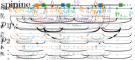
Figure 5: A fixation gadget for $F=2$ with five other pages in the stack layout. We also highlight the intended position for $f_{1}$ and $f_{2}$ on the spine and the page assignment for their incident edges.

Next, we show that the fixation gadget forces $f_{i}$ to lie between $v_{i}$ and $v_{i+1}$ on the spine and the edges $f_{i}v_{i}$ and $f_{i}v_{i+1}$ to be on the page $p_{d}$ for every $i\in[F]$.

Lemma 4.1.

Let $\mathcal{I}=\left(\ell,G,H,\langle\prec,\sigma\rangle\right)$ be an instance of SLE that contains a fixation gadget on $F$ vertices $\{f_{1},\ldots,f_{F}\}$. In any solution $\langle\prec_{G},\sigma_{G}\rangle$ to $\mathcal{I}$ and for every $i\in[F]$, we have $v_{i}\prec f_{i}\prec v_{i+1}$ and $\sigma(f_{i}v_{i})=\sigma(f_{i}v_{i+1})=p_{d}$. Furthermore, the fixation gadget contributes $4F+3$ vertices and $(\ell+4)F+\ell+2$ edges to the size of $\mathcal{I}$.

Towards establishing $v_{i}\prec f_{i}\prec v_{i+1}$, one can show that $f_{i}\prec v_{i}$ would prevent $f_{i}$ from seeing $v_{i+1}$ on any page: As $f_{i}\prec v_{i}$ implies $f_{i}\prec b_{i+1}\prec v_{i+1}\prec a_{i+1}$ and we have the edge $b_{i+1}a_{i+1}$ on any page except $p_{d}$, only visibility on page $p_{d}$ would still be possible. However, the edges on the page $p_{d}$ prevent visibility to $v_{i+1}$ for any spine position left of $v_{i}$. By symmetric arguments, we can obtain that $v_{i+1}\prec f_{i}$ would prevent $v_{i}$ from seeing $f_{i}$. Using again the fact that we have the edge $b_{i}a_{i}$ on any page except $p_{d}$, in concert with the relation $v_{i}\prec f_{i}\prec v_{i+1}$ shown above and the edges $v_{i}a_{i}$ and $b_{i+1}v_{i+1}$ on the page $p_{d}$, one can deduce that $\sigma(f_{i}v_{i})=\sigma(f_{i}v_{i+1})=p_{d}$ must hold. Finally, the bound on the size of the gadget can be obtained by a close analysis of the construction. plemmaFixationGadgetProperties Let $\langle\prec_{G},\sigma_{G}\rangle$ be a solution to $\mathcal{I}=\left(\ell,G,H,\langle\prec,\sigma\rangle\right)$. First, we will show that $v_{i}\prec f_{i}\prec v_{i+1}$ must hold. Towards a contradiction, assume that there exists a solution $\langle\prec_{G},\sigma_{G}\rangle$ with $f_{i}\prec v_{i}$. Observe that $f_{i}\prec v_{i}$ also implies $f_{i}\prec v_{i+1}$ and recall that we have in $H$ the edges $e(b_{i+1},a_{i+1},p)$ for every page $p\neq p_{d}$. As $b_{i+1}\prec_{H}v_{i+1}\prec_{H}a_{i+1}$ and $\langle\prec_{G},\sigma_{G}\rangle$ is an extension of $\langle\prec_{H},\sigma_{H}\rangle$, $f_{i}$ can see $v_{i+1}$ only on the page $p_{d}$. Hence, we must have $\sigma(f_{i}v_{i+1})=p_{d}$. We will now distinguish between the following two cases. On the one hand, there could exist a $j$ with $1\leq j<i\leq F$, such that $v_{j}\prec f_{i}\prec v_{j+1}\prec v_{i+1}$. However, since we have $\sigma_{H}(v_{j}v_{j+1})=p_{d}$, this cannot be the case, as this would introduce a crossing on the page $p_{d}$ between the edges $f_{i}v_{i+1}$ and $v_{j}v_{j+1}$. On the other hand, we could have $f_{i}\prec b_{1}$, i.e., $f_{i}$ is placed at the beginning of the fixation gadget. Observe that we have in this situation $f_{i}\prec b_{1}\prec v_{i+1}\prec a_{F+1}$ and $\sigma_{H}(b_{1}a_{F+1})=p_{d}$. Hence, we would introduce a crossing on the page $p_{d}$ between the edges $f_{i}v_{i+1}$ and $b_{1}a_{F+1}$. As $\sigma(f_{i}v_{i+1})=p_{d}$ can therefore not hold, we have no page to which we could assign $f_{i}v_{i+1}$ without introducing a crossing, contradicting the assumption that we have a solution with $f_{i}\prec v_{i}$. As the arguments that exclude $v_{i+1}\prec f_{i}$ are symmetric, we obtain that $v_{i}\prec f_{i}\prec v_{i+1}$ must hold in any solution to $\mathcal{I}$.

Secondly, we will show that $\sigma(f_{i}v_{i})=\sigma(f_{i}v_{i+1})=p_{d}$ holds. Towards a contradiction, assume that there exists a solution $\langle\prec_{G},\sigma_{G}\rangle$ with $\sigma(f_{i}v_{i})\neq p_{d}$ for some $i\in[F]$. Hence, $\sigma(f_{i}v_{i})=p$ holds for some page $p\neq p_{d}$. Recall that we have the edge $e(b_{i},a_{i},p)$ with $\sigma_{H}(e(b_{i},a_{i},p))=p$. This allows us to strengthen $v_{i}\prec f_{i}\prec v_{i+1}$, which we have shown before, to $v_{i}\prec f_{i}\prec a_{i}$ under the assumption of $\sigma(f_{i}v_{i})=p$, as we would otherwise have a crossing on the page $p$. However, then we can conclude from $\sigma_{H}(v_{i}a_{i})=p_{d}$ and the existence of the edges $e(b_{i+1},a_{i+1},p^{\prime})$, with $\sigma_{H}(e(b_{i+1},a_{i+1},p^{\prime}))=p^{\prime}$, for any page $p^{\prime}\neq p_{d}$ and $f_{i}\prec b_{i+1}\prec v_{i+1}\prec a_{i+1}$ that there does not exist a feasible page assignment for the edge $f_{i}v_{i+1}$. This contradicts our assumption of a solution with $\sigma(f_{i}v_{i})\neq p_{d}$ and a symmetric argument rules out any solution with $\sigma(f_{i}v_{i+1})\neq p_{d}$.

Thirdly, we analyze the size of the fixation gadget. Recall that $\mathcal{F}$ consists of $F$ vertices, and we introduce $3(F+1)$ vertices in $H$. Furthermore, the fixation gadget contributes one page to an (existing) stack layout $\langle\prec,\sigma\rangle$ of $H$ on $\ell-1$ pages. Regarding the number of edges, we create in $H$ $(\ell-1)(F+1)$ edges of the form $b_{i}a_{i}$, $i\in[F+1]$, $2(F+1)$ edges of the form $b_{i}v_{i}$ or $v_{i}a_{i}$, $i\in[F+1]$, $F$ edges of the form $v_{i}v_{i+1}$, $i\in[F]$, and the edge $b_{1}a_{F+1}$. Together with the $2F$ new edges that we add to $G$, this sums up to $(\ell+4)F+\ell+2$ edges. Lemma 4.1 tells us that we can restrict the feasible positions for $f_{i}$ to a pre-defined set of consecutive intervals by choosing suitable positions for $v_{i}$ and $v_{i+1}$ in the spine order $\prec_{H}$. As the fixation gadget requires an additional page $p_{d}$, we must ensure that the existence of the (otherwise mostly empty) page $p_{d}$ does not violate the semantics of our reductions. In particular, we will (have to) ensure that our full constructions satisfy the following property.

Property 1.

Let $\mathcal{I}=\left(\ell,G,H,\langle\prec,\sigma\rangle\right)$ be an instance of SLE that contains a fixation gadget on $F$ vertices $\{f_{1},\ldots,f_{F}\}$. In any solution $\langle\prec_{G},\sigma_{G}\rangle$ to $\mathcal{I}$ and for every new edge $e\in E_{\text{add}}{}$ with $\sigma(e)=p_{d}$, we have $e\in\{f_{i}v_{i},f_{i}v_{i+1}\mid i\in[F]\}$.

4.3 The Complete Reduction

Recall the base layout of our reduction that we described in Section 4.1 and illustrated with Figure 3. There, we created, for a given formula $\varphi$, one vertex for each variable $x_{i}$ and each clause $c_{j}$. Furthermore, each $x_{i}$ should only be visible on two pages that correspond to its individual truth state and each $c_{j}$ should only be visible on three pages that correspond to the complementary literals in $c_{j}$. However, the intended semantics of our reduction rely on the assumption that new vertices can only be placed on a specific position, and in a specific order, on the spine. Equipped with the fixation gadget, we will now satisfy this assumption.

For an instance $\varphi=(\mathcal{X},\mathcal{C})$ of 3-Sat, we take the base layout of our reduction as described in Section 4.1 and incorporate in $H$ a fixation gadget on two vertices, i.e., for $F=2$. We set $a_{3}\prec d_{1}$, i.e., we place the fixation gadget at the beginning of the spine, and identify $s=f_{1}$ and $v=f_{2}$. Furthermore, we add the edge $d_{1}d_{N+M+1}$ and set $\sigma(d_{1}d_{N+M+1})=p_{d}$. Observe that this ensures that our construction will have Property 1, as this edge prevents connecting $s$ with $x_{i}$ or $v$ with $c_{j}$ on page $p_{d}$ for any $i\in[N]$ and $j\in[M]$. Finally, we add to $G$ the new edges $sx_{i}$ and $vc_{j}$ for every $i\in[N]$ and $j\in[M]$. This completes our reduction and we establish with the following theorem its correctness; see also Figure 6 for an example of our construction for a small formula.

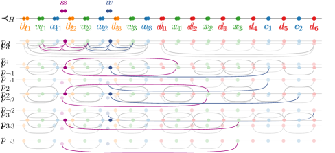
Figure 6: An example of our reduction for the formula $\varphi$ consisting of the clauses $c_{1}=\left(x_{1}\lor\lnot x_{2}\lor x_{3}\right)$ and $c_{2}=\left(\lnot x_{1}\lor x_{2}\lor x_{3}\right)$. The extension indicated in saturated colors induces the truth assignment $\Gamma(x_{1})=\Gamma(x_{2})=1$ and $\Gamma(x_{3})=0$, which satisfies $\varphi$.

Theorem 4.2.

SLE is -complete even if we have just two new vertices and $E_{\text{add}}^{H}{}=\emptyset$.

ptheoremParaNPHardness -membership of SLE follows immediately from the fact that we can encode a solution $\langle\prec,\sigma\rangle$ in $\mathcal{O}(\left|\mathcal{I}\right|)$ space and can verify it in polynomial time. Thus, we focus in the remainder of the proof on showing -hardness of SLE.

Let $\varphi=(\mathcal{X},\mathcal{C})$ be an instance of 3-Sat and let $\mathcal{I}=\left(\ell,G,H,\langle\prec,\sigma\rangle\right)$ be the obtained instance of SLE. The number of vertices and edges in $H$ that we created in the base layout of Section 4.1 is in $\mathcal{O}(N+M)$. Furthermore, in the base layout, we used $2N$ pages. Together with the page from the fixation gadget, we have $\ell=2N+1$. As $F=2$ is constant, the contribution of the fixation gadget to the size of $H$ and $G$ is linear in $\varphi$ by Lemma 4.1. Hence, the overall size of $\mathcal{I}$ is polynomial in the size of $\varphi$. Clearly, the time required to create $\mathcal{I}$ is also polynomial in the size of $\varphi$ and it remains to show the correctness of the reduction.

*($\boldsymbol{\Rightarrow}$) Assume that $\varphi$ is a positive instance of 3-Sat and let $\Gamma:\mathcal{X}\to\{0,1\}$ be a truth assignment that satisfies every clause. To show that $\mathcal{I}$ is a positive instance of SLE, we create a stack layout $\langle\prec,\sigma\rangle$ of $G$. We first ensure that it extends $\langle\prec_{H},\sigma_{H}\rangle$ by copying $\langle\prec_{H},\sigma_{H}\rangle$. Next, we set $a_{1}\prec s\prec b_{2}$, $a_{2}\prec v\prec b_{3}$ and $\sigma(sv_{1})=\sigma(sv_{2})=\sigma(vv_{2})=\sigma(vv_{3})=p_{d}$ as shown in Figure 6. Furthermore, for every variable $x_{i}\in\mathcal{X}$, we set $\sigma(sx_{i})=p_{i}$ if $\Gamma(x_{i})=1$ and $\sigma(sx_{i})=p_{\lnot i}$ otherwise. For every clause $c_{j}\in\mathcal{C}$, we identify a variable $x_{i}$ that satisfies the clause $c_{j}$ under $\Gamma$. As $\Gamma$ satisfies every clause, the existence of such an $x_{i}$ is guaranteed. Then, we set $\sigma(sx_{i})=p_{i}$ if $\Gamma(x_{i})=0$ and $\sigma(sx_{i})=p_{\lnot i}$ otherwise.

To show that $\langle\prec,\sigma\rangle$ is crossing-free, we first observe that for the fixation gadget, our generated solution satisfies the necessary properties stated in Lemma 4.1. We can observe that in our page assignment new edges cannot cross old edges. Hence, we only have to ensure that no two new edges cross. No two new edges on page $p_{d}$ can cross, so assume that there is a crossing on page $p_{i}$ for some $i\in[N]$. We observe that only edges of the form $sx_{i}$ and $vc_{j}$ for some $x_{i}\in\mathcal{X}$ and $c_{j}\in\mathcal{C}$ can cross, as they are otherwise incident to the same vertex. As there is a crossing on the page $p_{i}$, we must have by construction that the variable $x_{i}$ appears negated in the clause $c_{j}$ but we have $\Gamma(x_{i})=1$. Hence, $x_{i}$ does not satisfy $c_{j}$, which is a contradiction to our construction of $\langle\prec,\sigma\rangle$, for which we only considered variables that satisfy the clause $c_{j}$. Therefore, a crossing on the page $p_{i}$ cannot exist. As the argument for a crossing on page $p_{\lnot i}$ is symmetric, we conclude that $\langle\prec,\sigma\rangle$ must be crossing-free and hence witnesses that $\mathcal{I}$ is a positive instance of SLE.

*($\boldsymbol{\Leftarrow}$) Assume that $\mathcal{I}$ is a positive instance of SLE. This implies that there exists a witness extension $\langle\prec_{G},\sigma_{G}\rangle$ of $\langle\prec_{H},\sigma_{H}\rangle$. As $\mathcal{I}$ contains the fixation gadget, we can apply Lemma 4.1 and deduce that $s\prec v\prec d_{1}$ holds. Based on $\langle\prec_{G},\sigma_{G}\rangle$, we now construct a truth assignment $\Gamma\colon\mathcal{X}\to\{0,1\}$ for $\varphi$. For each variable $x_{i}\in\mathcal{X}$, we consider the page assignment $\sigma(sx_{i})$. Recall that we have $s\prec d_{1}\prec x_{i}\prec d_{N+M+1}$ and $\sigma_{H}(d_{1}d_{N+M+1})=p_{d}$. Together with $s\prec d_{i}\prec x_{i}\prec d_{i+1}$ and $\sigma_{H}(d_{i}d_{i+1})=p$ for any page $p\in[\ell]\setminus\{p_{d},p_{i},p_{\lnot i}\}$, we conclude that $\sigma(sx_{i})\in\{p_{i},p_{\lnot i}\}$ must hold. We set $\Gamma(x_{i})=1$ if $\sigma(sx_{i})=p_{i}$ holds and $\Gamma(x_{i})=0$ if $\sigma(sx_{i})=p_{\lnot i}$ holds and know by the above arguments that $\Gamma$ is well-defined. What remains to show is that $\Gamma$ satisfies $\varphi$. Let $c_{j}$ be an arbitrary clause of $\varphi$ and consider the page $p$ with $\sigma(vc_{j})=p$. As we have $\sigma_{H}(d_{1}d_{N+M+1})=p_{d}$ we know that $p\neq p_{d}$ must hold, i.e., the page $p$ is associated to some variable $x_{i}$. For the remainder of the proof, we assume $p=p_{i}$ as the case $p=p_{\lnot i}$ is symmetric. Recall that we have $d_{N+j}\prec_{H}c_{j}\prec_{H}d_{N+j+1}$, $\sigma_{H}(e(c_{j},p_{i^{\prime}}))=p_{i^{\prime}}$, and $\sigma_{H}(e(c_{j},p_{\lnot i^{\prime}}))=p_{\lnot i^{\prime}}$ for any variable $x_{i^{\prime}}\in\mathcal{X}$ that does not occur in $c_{j}$. Hence, we know that $x_{i}$ must occur in $c_{j}$. Furthermore, the same reasoning allows us to conclude that $x_{i}$ must appear negated in $c_{j}$, as we would otherwise have a crossing. Using $s\prec v\prec x_{i}\prec c_{j}$ and our assumption of $\sigma(vc_{j})=p_{i}$, we derive that $x_{i}$ will be visible from $s$ on page $p_{\lnot i}$ only, i.e., we have $\sigma(sx_{i})=p_{\lnot i}$. By our construction of $\Gamma$, we conclude $\Gamma(x_{i})=0$. Hence, $x_{i}$ satisfies $c_{j}$ under $\Gamma$. As $c_{j}$ was selected arbitrarily, this holds for all clauses and therefore must $\Gamma$ satisfy the whole formula $\varphi$, i.e., it witnesses that $\varphi$ is a positive instance of 3-Sat.

5 SLE Parameterized by Missing Vertices and Edges is in

In the light of Theorem 4.2, which excludes the use of the vertex+edge deletion distance as a pathway to tractability, we consider parameterizing by the total number of missing vertices and edges $\kappa\coloneqq n_{\text{add}}+m_{\text{add}}$. As our first result in this direction, we show that parameterizing SLE by $\kappa$ makes it -tractable. To this end, we combine a branching-procedure with the fixed parameter algorithm for the special case obtained in Theorem 3.2.

Theorem 5.1.

Let $\mathcal{I}=\left(\ell,G,H,\langle\prec,\sigma\rangle\right)$ be an instance of SLE. We can find an $\ell$-page stack layout of $G$ that extends $\langle\prec,\sigma\rangle$ or report that none exists in $\mathcal{O}(\left|\mathcal{I}\right|^{n_{\text{add}}+1}{m_{\text{add}}}^{m_{\text{add}}})$ time.

Proof 5.2.

We branch over the possible assignments of new vertices to the intervals in $\prec_{H}$. As a solution could assign multiple vertices to the same interval, we also branch over the order in which all vertices will appear in the spine order $\prec_{G}$. Observe that $\prec_{H}$ induces $\left|V(H)\right|+1$ different intervals, out of which we have to choose $n_{\text{add}}{}$ with repetition. Together with the possible orders of the new vertices, we can bound the number of branches by $n_{\text{add}}{}!\cdot\binom{\left|V(H)\right|+n_{\text{add}}{}}{n_{\text{add}}{}}$. We can simplify this expression to

$$\frac{n_{\text{add}}{}!\cdot(\left|V(H)\right|+n_{\text{add}}{})!}{n_{\text{add}}{}!\cdot((\left|V(H)\right|+n_{\text{add}}{})-n_{\text{add}}{})!}=\frac{(\left|V(H)\right|+n_{\text{add}}{})!}{\left|V(H)\right|!}=\Pi_{i=1}^{n_{\text{add}}{}}(\left|V(H)\right|+i)=\mathcal{O}(\left|\mathcal{I}\right|^{n_{\text{add}}{}}).$$

In each branch, the spine order $\prec_{G}$ is fixed and extends $\prec_{H}$. Hence, it only remains to check whether $\prec_{G}$ allows for a valid page assignment $\sigma_{G}$. As each branch corresponds to an instance of SLE where only edges are missing, we use Theorem 3.2 to check in $\mathcal{O}({m_{\text{add}}{}}^{m_{\text{add}}{}}\cdot\left|\mathcal{I}\right|)$ time whether such an assignment $\sigma_{G}$ exists. The overall running time now follows readily.

The running time stated in Theorem 5.1 not only proves that SLE is in when parameterized by $\kappa$, but also when parameterized by $m_{\text{add}}{}$ for constant $n_{\text{add}}{}$. However, common complexity assumptions rule out an efficient algorithm parameterized by $\kappa$, as we show next.

6 SLE Parameterized by Missing Vertices and Edges is [1]-hard

In this section, we show that SLE parameterized by the number $\kappa$ of missing vertices and edges is [1]-hard. To show [1]-hardness, we reduce from the Multi-colored Clique (McC) problem. Here, we are given a graph $G_{C}$, an integer $k>0$, and a partition of $V(G_{C})$ into $k$ independent subsets $V_{1},\ldots,V_{k}$, and ask whether there exists a colorful $k$-clique $\mathcal{C}\subseteq V(G_{C})$ in $G_{C}$, i.e., a clique on $k$ vertices that contains exactly one vertex of every set $V_{i}$, $i\in[k]$. It is known that McC is [1]-hard when parameterized by $k$ [15]. In the following, we will use Greek letters for the indices of the partition and denote with $n_{\alpha}$ the number of vertices in $V_{\alpha}$, i.e., $n_{\alpha}=\left|V_{\alpha}\right|$. Observe that $\sum_{\alpha\in[k]}n_{\alpha}=N$ with $N=\left|V(G_{C})\right|$. As we can interpret the partitioning of the vertices into $V_{1},\ldots,V_{k}$ as assigning to them one of $k$ colors, we will call a vertex $v_{\alpha}^{i}$ with $\alpha\in[k]$ and $i\in[n_{\alpha}]$ a vertex with color $\alpha$. Our construction will heavily use the notion of a successor and predecessor of a vertex in a given spine order $\prec$. For a vertex $u$, the function $\text{succ}(\prec,\ u)$ returns the successor of $u$ in the spine order $\prec$, i.e., the consecutive vertex in $\prec$ after $u$. Note that $\text{succ}(\prec,\ u)$ is undefined if there is no vertex $v\in V(G)$ with $u\prec v$. We write $\text{succ}(u)$ if $\prec$ is clear from context. The predecessor function $\text{pred}(\prec,\ u)$ is defined analogously. mccIntro

Let $(G_{C},k,(V_{1},\ldots,V_{k}))$ be an instance of McC. We will construct an SLE instance $\left(\ell,G,H,\langle\prec,\sigma\rangle\right)$ parameterized by $\kappa$ that will fulfill two crucial properties to ensure its correctness. While, at the time of stating the property, our construction might not yet fulfill it, we show in Section 6.4 that in the end it indeed has the desired properties. Our instance contains for every original vertex $v_{\alpha}^{i}\in V(G_{C})$ a copy $u_{\alpha}^{i}\in V(H)$. Furthermore, we add for each color $\alpha\in[k]$ to $H$ two additional vertices and, overall, three further dummy vertices that we use to ensure correctness of the reduction. We place the vertices on the spine based on their color $\alpha$ and index $i$; see Figure 7 and Section 6.1, where we give the full details of the base layout. Observe that every vertex $v_{\alpha}^{i}\in V(G_{C})$ induces the interval $[u_{\alpha}^{i},u_{\alpha}^{i+1}]$ in $\prec_{H}$, which we denote with $\curlyvee(v_{\alpha}^{i})$. The equivalence between the two problems will be obtained by adding a $k$-clique to $G$ that consists of the $k$ new vertices $\mathcal{X}=\{x_{1},\ldots,x_{k}\}$. Placing $x_{\alpha}\in\mathcal{X}$ in $\curlyvee(v_{\beta}^{i})$ indicates that $v_{\beta}^{i}$ will be part of the colorful $k$-clique in $G_{C}$.

To establish the correctness of our reduction, we have to ensure two things. First, we have to model the adjacencies in $G_{C}$. In particular, two new vertices $x_{\alpha}$ and $x_{\beta}$, with $\alpha<\beta$, should only be placed in intervals induced by vertices adjacent in $G_{C}$. We enforce this by adding for every edge $e=v_{\alpha}^{i}v_{\beta}^{j}\in E(G_{C})$ a page $p_{e}$ that contains a set of edges creating a tunnel on $p_{e}$, see Figure 8, and thereby allowing us to place the edge $x_{\alpha}x_{\beta}\in E(G)$ in the page $p_{e}$ if and only if $x_{\alpha}$ is placed in $\curlyvee(v_{\alpha}^{i})$ and $x_{\beta}$ in $\curlyvee(v_{\beta}^{j})$. Hence, the page assignment verifies that only pairwise adjacent vertices are in the solution, i.e., new vertices can only be placed in intervals induced by a clique in $G_{C}$. We describe the tunnel further in Section 6.2.

Second, we have to ensure that we select exactly one vertex $v_{\alpha}^{i}\in V_{\alpha}$ for every color $\alpha\in[k]$. In particular, the new vertex $x_{\alpha}$ should only be placed in intervals that are induced by vertices from $V_{\alpha}$. To this end, we modify $H$ to include an appropriate fixation gadget by re-using some vertices of the base layout; see Section 6.3 for details. As the whole base layout thereby forms the fixation gadget, our construction trivially satisfies Property 1.

The above two ideas are formalized in Properties 2 and 3. With these properties at hand, we show at the end of Section 6.4 that SLE is [1]-hard when parameterized by $\kappa$.

As in the reduction from Section 4, we will allow multi-edges in the graph $H$ to facilitate presentation and understanding. In Section A.3 we will discuss a way to remove the multi-edges by distributing the individual edges over auxiliary vertices.

sectionWOneBaseLayout

6.1 Creating Intervals on the Spine: Our Base Layout

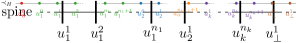
Figure 7: The base layout of our reduction. We use colors to additionally differentiate vertices that originate from different vertex sets $V_{\alpha}$, for $\alpha\in[k]$, and the dummy vertices $u_{0}^{0}$, $u_{\bot}^{0}$ and $u_{\bot}^{1}$.

Recall that $G_{C}$ has the vertex set $V(G_{C})=\{v_{1}^{1},\ldots,v_{k}^{n_{k}}\}$ partitioned into $V_{1},\ldots,V_{k}$ with $V_{\alpha}=\{v_{\alpha}^{1},\ldots,v_{\alpha}^{n_{\alpha}}\}$ for ${\alpha}\in[k]$. We create the $N+2k+3$ vertices $\{u_{\alpha}^{j}\mid{\alpha}\in[k],\ j\in[n_{\alpha}+1]_{0}\}\cup\{u_{0}^{0},u_{\bot}^{0},u_{\bot}^{1}\}$ in $H$. Note that for each original vertex $v_{\alpha}^{i}\in V(G_{C})$, we have a copy $u_{\alpha}^{i}$. We will refer to the vertices $u_{0}^{0}$, $u_{\bot}^{0}$, and $u_{\bot}^{1}$ as dummy vertices and set, for ease of notation, $\bot=k+1$ and $n_{\bot}=1$. We order the vertices of $H$ on the spine by setting $u_{\alpha}^{i}\prec u_{\alpha}^{i+1}$ and $u_{\alpha}^{n_{\alpha}+1}\prec u_{\alpha+1}^{0}$ for every $\alpha\in[k]$ and $i\in[n_{\alpha}]_{0}$. Furthermore, we set $u_{0}^{0}\prec u_{1}^{0}$ and $u_{\bot}^{0}\prec u_{\bot}^{1}$. The spine order is then the transitive closure of the above partial orders. We visualize it in Figure 7 and observe that $\text{succ}(u_{\alpha}^{i})=u_{\alpha}^{i+1}$ for every $v_{\alpha}^{i}\in V(G_{C})$.

As already indicated, we define the set $\mathcal{X}=\{x_{1},\ldots,x_{k}\}$ to contain $k$ (new) vertices which we add to $G$. Furthermore, we form a $k$-clique on $\mathcal{X}$, i.e., we add the edges $x_{\alpha}x_{\beta}$ for $1\leq\alpha<\beta\leq k$ to $E(G)$. Recall that $\curlyvee(v_{\alpha}^{i})$ denotes the interval $[u_{\alpha}^{i},\text{succ}(\prec_{H},\ u_{\alpha}^{i})]$. We use the following equivalence between a solution $\langle\prec_{G},\sigma_{G}\rangle$ to SLE and a solution $\mathcal{C}$ to McC.

$$u_{\alpha}^{i}\prec x_{\alpha}\prec\text{succ}(\prec_{H},\ u_{\alpha}^{i})\ \overset{\text{p.\leavevmode\nobreak\ d.}}{\Longleftrightarrow}\ x_{\alpha}\ \text{is placed in}\ \curlyvee(v_{\alpha}^{i})\ \Longleftrightarrow\ v_{\alpha}^{i}\in\mathcal{C}$$ (1)

To guarantee that $\mathcal{C}$ is colorful, i.e., contains exactly one vertex from each color, we will ensure the following property with our construction.

Property 2.

In a solution $\langle\prec,\sigma\rangle$ to SLE we have $u_{\alpha}^{0}\prec x_{\alpha}\prec u_{\alpha+1}^{0}$ for every $\alpha\in[k]$.

Of course, our construction does not yet fulfill Property 2. We will show in Section 6.4 that the finished construction indeed does fulfill Property 2.

sectionWOneEdges

6.2 Creating One Page Per Edge: Encoding the Adjacencies

Having fixed the base order on the spine, we now ensure that we only select vertices that are adjacent in $G_{C}$, i.e., we encode the edges of $G_{C}$ in our stack layout $\langle\prec_{H},\sigma_{H}\rangle$. Let $e=v_{\alpha}^{i}v_{\beta}^{j}$ be an edge of $G_{C}$ and recall that, by our assumption, we have $\alpha\neq\beta$. Furthermore, we assume for ease of presentation that $\alpha<\beta$ holds, which implies $u_{\alpha}^{i}\prec u_{\beta}^{j}$. We create the following edges in $H$; see Figure 8. Note that each of the them is assigned to the page $p_{e}$ in $\sigma$, where $p_{e}$ is a new empty page that we associate with the edge $e$. Firstly, we create the edge $u_{\gamma}^{1}u_{\gamma}^{n_{\gamma}+1}$ for each $\gamma\in[k]\setminus\{\alpha,\beta\}$; see Figure 8a. Secondly, we create the edges $u_{\alpha}^{1}u_{\alpha}^{i}$ and $u_{\alpha}^{i+1}u_{\alpha}^{n_{\alpha}+1}$ as shown in Figure 8b. Similarly, we add the edges $u_{\beta}^{1}u_{\beta}^{j}$ and $u_{\beta}^{j+1}u_{\beta}^{n_{\beta}+1}$. If $i\in\{1,n_{\alpha}\}$ or $j\in\{1,n_{\beta}\}$, we omit creating the respective edge to not introduce self-loops in $H$. Thirdly, we create the edges $u_{\alpha}^{i}u_{\beta}^{j+1}$ and $u_{\alpha}^{i+1}u_{\beta}^{j}$, which we mark in Figure 8c in black.

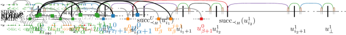
Figure 8: Edges of $H$ that model the adjacency given by the edge $e=v_{\alpha}^{i}v_{\beta}^{j}\in E(G_{C})$. All of these edges are placed on the page $p_{e}$. Intuitively, we span the intervals induced (a) by all vertices for each color $\gamma\in[\kappa]\setminus\{\alpha,\beta\}$ and (b) by vertices of the colors $\alpha$ and $\beta$ that are not incident to $e$, here visualized for the color $\alpha$. (c) Furthermore, we create a tunnel that connects $\curlyvee(v_{\alpha}^{i})$ with $\curlyvee(v_{\beta}^{j})$. The gray edges in (c) are from (a) and (b).

One can readily verify that these edges in the page $p_{e}$ do not cross. Furthermore, observe that the edges $u_{\alpha}^{i}u_{\beta}^{j+1}$ and $u_{\alpha}^{i+1}u_{\beta}^{j}$ create a tunnel on the page $p_{e}$ connecting $\curlyvee(v_{\alpha}^{i})$ and $\curlyvee(v_{\beta}^{j})$. Intuitively, the edges on the page $p_{e}$ ensure that if $x_{i}$ is placed in $\curlyvee(v_{\alpha}^{i})$ then $x_{i}$ sees only $\curlyvee(v_{\beta}^{j})$ on page $p_{e}$. More formally, we will have the following property.

Property 3.

Let $\langle\prec,\sigma\rangle$ be a solution to an instance of SLE that fulfills Property 2 and for which we have $e=v_{\alpha}^{i}v_{\beta}^{j}\in E(G_{C})$, $1\leq\alpha<\beta\leq k$, and $x_{\alpha},x_{\beta}\in\mathcal{X}$. If $\sigma(x_{\alpha}x_{\beta})=p_{e}$ then $x_{\alpha}$ is in $\curlyvee(v_{\alpha}^{i})$ and $x_{\beta}$ is in $\curlyvee(v_{\beta}^{j})$.

sectionWOneFixationGadget

6.3 Restricting The Placement of New Vertices: Encoding the Colors

Until now, the new vertices in $\mathcal{X}$ can be placed in any interval on the spine. However, in McC we must select exactly one vertex from each color. Recall Property 2, which intuitively states that each new vertex should only be placed in intervals that correspond to its color. We now use the fixation gadget to ensure that our construction fulfills Property 2. Observe that we already introduced in Section 6.1 the required vertices of the fixation gadget when creating the base layout of our reduction. More specifically, we (implicitly) create in $H$ and our construction the fixation gadget on $F=k$ vertices $\mathcal{F}=\mathcal{X}$ by identifying, for $\alpha\in[k+1]$, $v_{i}=u_{\alpha}^{0}$, $b_{i}=\text{pred}(u_{\alpha^{0}})$, and $a_{i}=\text{succ}(u_{\alpha}^{0})$, where we use $i=\alpha$ to differentiate between the vertices from the fixation gadget and the graphs $G_{C}$ and $H$. We also introduce the corresponding edges of the fixation gadget, which we visualize for the vertices in this construction in Figure 9.

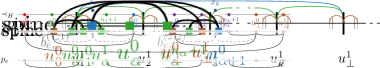
Figure 9: We use a fixation gadget to encode the color constraints. This figure is an adapted version of Figure 5 that shows the fixation gadget on $k$ vertices with the vertices used in this reduction. We visualize the dummy page $p_{d}$ and a page $p_{e}$ created for an edge $e\in E(G_{C})$.

Recall that when introducing the fixation gadget in Section 4.2, we required that our instance must fulfill Property 1, which states that $p_{d}$ must only be used by new edges that were introduced in the fixation gadget. However, observe that any new edge $e\in E(G)\setminus(E(H)\cup\{x_{\alpha}u_{\alpha}^{0},x_{\alpha}u_{\alpha+1}^{0}\mid\alpha\in[k]\})$, i.e., that was not introduced in the fixation gadget, is of the form $e=x_{\alpha}x_{\beta}$ for $1\leq\alpha<\beta\leq k$, i.e., one of the edges in the $k$-clique. Lemma 4.1 tells us that for every new vertex $x_{\alpha}\in\mathcal{X}$ we have $u_{\alpha}^{0}\prec x_{\alpha}\prec u_{\alpha+1}^{0}$ in any extension $\langle\prec_{G},\sigma_{G}\rangle$ of $\langle\prec_{H},\sigma_{H}\rangle$. This implies that we have $u_{\alpha}^{0}\prec x_{\alpha}\prec u_{\alpha+1}^{0}\preceq u_{\beta}^{0}\prec x_{\beta}\prec u_{\beta+1}^{0}$. Together with having $u_{\alpha}^{0}u_{\alpha+1}^{0},u_{\beta}^{0}u_{\beta+1}^{0}\in E(H)$ and $\sigma_{H}(u_{\alpha}^{0}u_{\alpha+1}^{0})=\sigma(u_{\beta}^{0}u_{\beta+1}^{0})=p_{d}$, this rules out $\sigma_{G}(x_{\alpha}x_{\beta})=p_{d}$. Hence, we observe that the fixation gadget is formed on the base layout and our construction thus (trivially) fulfills Property 1.

6.4 Bringing It Together: Showing Correctness of the Reduction

We start by shortly summarizing our construction. Recall that we want to insert $k$ new vertices that form a clique. On a high level, we first created for each vertex $v_{\alpha}^{i}\in V(G_{C})$ a copy $u_{\alpha}^{i}\in V(H)$ and ordered the latter vertices depending on the color $\alpha$ and the index $i$. Then, we created for each edge $e\in E(G_{C})$ a page $p_{e}$ on which we formed a tunnel that will enforce for every new edge assigned to $p_{e}$ that its endpoints lie in specific intervals via Property 3. Finally, we used the fixation gadget to ensure that a new vertex can only be placed in intervals for its color, i.e., that our construction will enforce Property 2. Overall, we obtain for an instance $(G_{C},k,(V_{1},\ldots,V_{k}))$ of McC an instance $\mathcal{I}{}=\left(\ell,G,H,\langle\prec,\sigma\rangle\right){}$ of SLE that we parameterize by the number $\kappa$ of missing vertices and edges. Before we show correctness of the reduction, we first argue in Sections 6.4 and 6.2 that $\mathcal{I}$ fulfills Properties 2 and 3, respectively. Recall that Property 2 is defined as follows. See 2 In Section 6.3, when incorporating the fixation gadget on $F=k$ vertices in our construction, we identified $v_{i}=u_{\alpha}^{0}$ and $f_{i}=x_{\alpha}$ for every $\alpha\in[k]$ and $i=\alpha$. Similarly, we identified $v_{F+1}=u_{k+1}^{0}$. The fixation gadget now guarantees thanks to Lemma 4.1 that we have $v_{\alpha}\prec_{G}f_{\alpha}\prec_{G}v_{\alpha+1}$, i.e., $u_{\alpha}^{0}\prec x_{\alpha}\prec u_{\alpha+1}^{0}$, in any solution $\langle\prec_{G},\sigma_{G}\rangle$. Hence, we can observe the following. Our instance $\mathcal{I}$ of SLE fulfills Property 2. Recall that Lemma 4.1 furthermore tells us that we have in any solution $\langle\prec_{G},\sigma_{G}\rangle$ the page assignment $\sigma(x_{\alpha}u_{\alpha}^{0})=\sigma(x_{\alpha}u_{\alpha+1}^{0})=p_{d}$ for every $\alpha\in[k]$. As we have by Property 2 $u_{\alpha}^{0}\prec x_{\alpha}\prec u_{\alpha+1}^{0}$ and furthermore by the construction of the fixation gadget $\sigma_{H}(\text{pred}(u_{\alpha}^{0})u_{\alpha}^{0})=\sigma_{H}(u_{\alpha}^{0}\text{succ}(u_{\alpha}^{0}))=p_{d}$ for every $\alpha\in[k]$, we cannot have in $\langle\prec_{G},\sigma_{G}\rangle$ $u_{\alpha}^{0}\prec x_{\alpha}\prec\text{succ}(\prec_{H},\ u_{\alpha}^{0})$ or $\text{pred}(\prec_{H},\ u_{\alpha+1}^{0})\prec x_{\alpha}\prec u_{\alpha+1}^{0}$, as this would introduce a crossing on page $p_{d}$. As we have in $\prec_{H}$ the equality $\text{succ}(u_{\alpha}^{0})=u_{\alpha}^{1}$ and $\text{pred}(u_{\alpha+1}^{0})=u_{\alpha}^{n_{\alpha}+1}$ for every $\alpha\in[k]$, we can strengthen Property 2 and obtain the following.

Corollary 6.1.

In a solution $\langle\prec,\sigma\rangle$ to SLE we have $u_{\alpha}^{1}\prec x_{\alpha}\prec u_{\alpha}^{n_{\alpha}+1}$ for every $\alpha\in[k]$.

Finally, we now show that our construction fulfills Property 3, which was defined as follows.

See 3

Lemma 6.2.

Our instance $\mathcal{I}$ of SLE fulfills Property 3.

Proof 6.3.

First, recall that we made Section 6.4, i.e., our construction fulfills Property 2. Let $\langle\prec_{G},\sigma_{G}\rangle$ be a solution to SLE with $\sigma(x_{\alpha}x_{\beta})=p_{e}$, for $e=v_{\alpha}^{i}v_{\beta}^{j}\in E(G_{C})$, $1\leq\alpha<\beta\leq k$. Corollary 6.1 tells us that $u_{\alpha}^{1}\prec x_{\alpha}\prec u_{\alpha}^{n_{\alpha}+1}$ and $u_{\beta}^{1}\prec x_{\beta}\prec u_{\beta}^{n_{\beta}+1}$ holds. Corollary 6.1 also holds for any new vertices $x_{\gamma}$ and $x_{\delta}$ with $\gamma,\delta\in[k]\setminus\{\alpha,\beta\}$ and $\gamma\neq\delta$. Furthermore, we have the edges $u_{\gamma}^{1}u_{\gamma}^{n_{\gamma}+1}$ and $u_{\delta}^{1}u_{\delta}^{n_{\delta}+1}$ on page $p_{e}$. Hence, all new edges on page $p_{e}$ must be among new vertices placed in intervals induced by vertices of color $\alpha$ or $\beta$.

Now assume that we have $u_{\alpha}^{1}\preceq x_{\alpha}\preceq u_{\alpha}^{i}$. Using $\sigma_{H}(u_{\alpha}^{1}u_{\alpha}^{i})=p_{e}$ together with $u_{\alpha}^{1}\preceq x_{\alpha}\preceq u_{\alpha}^{i}\prec x_{\beta}$, we derive that $u_{\alpha}^{1}\preceq x_{\alpha}\preceq u_{\alpha}^{i}$ results in a crossing on page $p_{e}$. Hence, $u_{\alpha}^{1}\preceq x_{\alpha}\preceq u_{\alpha}^{i}$ cannot hold. Now assume that we have $u_{\alpha}^{i+1}\preceq x_{\alpha}\preceq u_{\alpha}^{n_{\alpha}+1}$. From $\sigma_{H}(u_{\alpha}^{i+1}u_{\alpha}^{n_{\alpha}+1})=p_{e}$ and $u_{\alpha}^{i+1}\preceq x_{\alpha}\preceq u_{\alpha}^{n_{\alpha}+1}\prec x_{\beta}$ we get that $u_{\alpha}^{i+1}\preceq x_{\alpha}\preceq u_{\alpha}^{n_{\alpha}+1}$ results in a crossing on page $p_{e}$. Hence, $u_{\alpha}^{i+1}\preceq x_{\alpha}\preceq u_{\alpha}^{n_{\alpha}+1}$ cannot hold. Since we can exclude $u_{\alpha}^{1}\preceq x_{\alpha}\preceq u_{\alpha}^{i}$ and $u_{\alpha}^{i+1}\preceq x_{\alpha}\prec u_{\alpha}^{n_{\alpha}+1}$ by the construction of the tunnel on page $p_{e}$, we can derive that $x_{\alpha}$ must be placed in $\curlyvee(v_{\alpha}^{i})$. As similar arguments can be made for $x_{\beta}$, we can conclude that we get a crossing on page $p_{e}$ unless $x_{\alpha}$ is placed in $\curlyvee(v_{\alpha}^{i})$ and $x_{\beta}$ in $\curlyvee(v_{\beta}^{i})$.

We are now ready to show correctness of our reduction, i.e., show the following theorem.

Theorem 6.4.

SLE parameterized by the number $\kappa$ of missing vertices and edges is [1]-hard.

Let $(G_{C},k,(V_{1},\ldots,V_{k}))$ be an instance of McC with $N=\left|V(G_{C})\right|$ and $M=\left|E(G_{C})\right|$ and let $\mathcal{I}{}=\left(\ell,G,H,\langle\prec,\sigma\rangle\right){}$ be the instance of SLE parameterized by the number $\kappa$ of missing vertices and edges created by our construction described above. Closer analysis reveals that the size of $\mathcal{I}$ is bounded by $\mathcal{O}(N+Mk+k^{2})$, and we have $\kappa=3k+\binom{k}{2}$ as $n_{\text{add}}{}=k$ and $m_{\text{add}}{}=\binom{k}{2}+2k$; recall that the fixation gadget contributes $2k$ new edges.

Towards arguing correctness, assume that $(G_{C},k,(V_{1},\ldots,V_{k}))$ contains a colorful $k$-clique $\mathcal{C}$. We construct a solution to $\mathcal{I}$ by, for every new vertex $x_{\alpha}\in\mathcal{X}$, considering the vertex $v_{\alpha}^{i}\in\mathcal{C}$ and placing $x_{\alpha}$ immediately to the right of the copy $u_{\alpha}^{i}$ of $v_{\alpha}^{i}$ in $H$. The fact that $\mathcal{C}$ is a clique then guarantees that, for each edge $e\in E(G_{C}[\mathcal{C}])$, there exists the page $p_{e}$ in which the corresponding edge $e^{\prime}\in E(G[\mathcal{X}])$ can be placed in. For the remaining edges from the fixation gadget, we can use the page assignment from Lemma 4.1.

For the converse (and more involved) direction, assume that SLE admits a solution $\langle\prec_{G},\sigma_{G}\rangle$. By Property 2, we have that each $x_{\alpha}\in V_{\text{add}}$ must be placed between $u_{\alpha}^{0}$ and $u_{\alpha+1}^{0}$. Moreover, our construction together with the page assignment forced by Lemma 4.1 guarantees that $x_{\alpha}$ is placed between precisely one pair of consecutive vertices $u_{\alpha}^{i_{\alpha}}$ and $u_{\alpha}^{i_{\alpha}+1}$, for some $i_{\alpha}\in[n_{\alpha}]$; recall Corollary 6.1. Our solution $\mathcal{C}$ to the instance of McC will consist of the vertices $v_{\alpha}^{i_{\alpha}}$, i.e., exactly one vertex per color $\alpha$. Moreover, each new edge $x_{\alpha}x_{\beta}\in E(G[\mathcal{X}])$ must be placed by $\sigma_{G}$ on some page, and as our construction satisfies Properties 1 and 3, this page must be one that is associated to one edge $e=v_{\alpha}^{i_{\alpha}}v_{\beta}^{i_{\beta}}$ of $G_{C}$. Property 3 now also guarantees that this page assignment enforces that $x_{\alpha}$ and $x_{\beta}$ are placed precisely between the consecutive vertices $u_{\alpha}^{i_{\alpha}}$ and $u_{\alpha}^{i_{\alpha}+1}$ and $u_{\beta}^{i_{\beta}}$ and $u_{\beta}^{i_{\beta}+1}$ of $H$, respectively. This means that the vertices in $\mathcal{C}$ are pairwise adjacent, which implies that $\mathcal{C}$ is a colorful $k$-clique. ptheoremWOne Let $(G_{C},k,(V_{1},\ldots,V_{k}))$ be an instance of McC with $N=\left|V(G_{C})\right|$ and $M=\left|E(G_{C})\right|$. Furthermore, let $\mathcal{I}{}=\left(\ell,G,H,\langle\prec,\sigma\rangle\right){}$ be the instance of SLE parameterized by the number $\kappa$ of missing vertices and edges created by our construction described above.

We first bound the size of $\mathcal{I}$ and note that we create $N+2k+3$ vertices in $H$ in Section 6.2 and $k$ additional new vertices in $G$ in Section 6.1. We enrich $H$ by $k+4$ edges for each edge $e\in E(G_{C})$. This gives us $M\left(k+4\right)$ edges in $H$ so far. Furthermore, in Section 6.3, we use a fixation gadget to keep the new vertices in place. As we introduce for the fixation gadget no new vertex but rather identify vertices of the fixation gadget with already introduced ones from $H$, it only remains to account for the edges of the gadget, which are $(M+5)k+M+3$; see Lemma 4.1 and note that $\langle\prec_{H},\sigma_{H}\rangle$ has $\ell=M+1$ pages as we create one page for each edge in $G_{C}$ and have the dummy page from the fixation gadget. Finally, we also add a clique among the $k$ new vertices, which are $\binom{k}{2}$ additional edges. Overall, the size of $H$ and $G$ is therefore in $\mathcal{O}(N+Mk+k^{2})$. Hence, the size of the constructed instance is polynomial in the size of $G_{C}$ and the new parameters are bounded by a (computable) function of the old parameter, more specifically, we have $n_{\text{add}}{}=k$ and $m_{\text{add}}{}=\binom{k}{2}+2k$, thus $\kappa=3k+\binom{k}{2}$. The instance $\mathcal{I}$ can trivially be created in ($\kappa$)-time. We conclude with showing the correctness of our construction.

*($\boldsymbol{\Rightarrow}$) Let $(G_{C},k,(V_{1},\ldots,V_{k}))$ be a positive instance of McC with solution $\mathcal{C}=\{v_{1}^{i},\ldots,v_{k}^{j}\}$. We construct a witness extension $\langle\prec_{G},\sigma_{G}\rangle$ of $\langle\prec_{H},\sigma_{H}\rangle$ to show that $\mathcal{I}$ is a positive instance of SLE. First, we copy $\langle\prec_{H},\sigma_{H}\rangle$ to ensure that $\langle\prec_{G},\sigma_{G}\rangle$ extends $\langle\prec_{H},\sigma_{H}\rangle$. Then, we extend $\langle\prec_{G},\sigma_{G}\rangle$ as follows.

For every $v_{\alpha}^{i}\in\leavevmode\nobreak\ \mathcal{C}$, we set $u_{\alpha}^{i}\prec x_{\alpha}\prec u_{\alpha}^{i+1}$. We also set $\sigma(x_{\alpha}u_{\alpha}^{0})=\sigma(x_{\alpha}u_{\alpha+1}^{0})=\leavevmode\nobreak\ p_{d}$. For every $x_{\alpha},x_{\beta}\in\mathcal{X}$ with $1\leq\alpha<\beta\leq k$ let $x_{\alpha}$ be placed in $\curlyvee(v_{\alpha}^{i})$ and $x_{\beta}$ be placed in $\curlyvee(v_{\beta}^{j})$. We set $\sigma(x_{\alpha}x_{\beta})=p_{e}$ for the edge $e=v_{\alpha}^{i}v_{\beta}^{j}$. As $\mathcal{C}$ is a clique, we must have $v_{\alpha}^{i}v_{\beta}^{j}\in E(G_{C})$ and thus we have the page $p_{e}$ in $\mathcal{I}$, i.e., this page assignment is well-defined. This completes the creation of $\langle\prec_{G},\sigma_{G}\rangle$. As it is an extension of $\langle\prec_{H},\sigma_{H}\rangle$ by construction, we only show that no two edges on the same page cross.

It is trivial that no two new edges, i.e., edges from $E_{\text{add}}$ can cross as they are all put on different pages. For the edges $x_{\alpha}u_{\alpha}^{0}$ and $x_{\alpha}u_{{\alpha}+1}^{0}$ it is sufficient to observe that we assemble the necessary page assignment from Lemma 4.1. What remains to do is to analyze edges of the form $x_{\alpha}x_{\beta}$. Recall that we set $\sigma(x_{\alpha}x_{\beta})=p_{e}$ for $e=v_{\alpha}^{i}v_{\beta}^{j}$ and $x_{\alpha}$ is placed in $\curlyvee(v_{\alpha}^{i})$ and $x_{\beta}$ is placed in $\curlyvee(v_{\beta}^{j})$. To see that there does not exist an old edge $e^{\prime}=uv\in E(H)$ that crosses $e$, i.e., with $\sigma(e^{\prime})=p_{e}$ and $u\prec x_{\alpha}\prec v\prec x_{\beta}$, recall that the only old edge $e^{\prime}=uv$ on the page $p_{e}$ for which we have $u\prec x_{\alpha}\prec v$ is the edge $e^{\prime}=u_{\alpha}^{i}u_{\beta}^{j+1}$ but we have $x_{\beta}\prec u_{\beta}^{j+1}$, i.e., the edge $e^{\prime}$ “spans over” the edge $x_{\alpha}x_{\beta}$. As a similar argument can be made to show that there cannot exist an edge $e^{\prime}=uv\in E(H)$ with $\sigma(e^{\prime})=p_{e}$ and $x_{\alpha}\prec u\prec x_{\beta}\prec v$, we conclude that there are no crossings on the page $p_{e}$.

As all edges are covered by these cases, we conclude that no two edges of the same page in $\langle\prec_{G},\sigma_{G}\rangle$ can cross, i.e., $\langle\prec_{G},\sigma_{G}\rangle$ is a witness that $\mathcal{I}$ is a positive instance of SLE.

*($\boldsymbol{\Leftarrow}$) Let $\mathcal{I}$ be a positive instance of SLE. Hence, their exists a stack layout $\langle\prec_{G},\sigma_{G}\rangle$ that extends $\langle\prec_{H},\sigma_{H}\rangle$. We now construct, based on $\langle\prec_{G},\sigma_{G}\rangle$, a set $\mathcal{C}$ of $k$ vertices and show that it forms a colorful clique in $G_{C}$. Recall that $\mathcal{I}$ fulfills Properties 2 and 3 and contains the fixation gadget. From Property 2 and Corollary 6.1, we conclude that we have $u_{\alpha}^{1}\prec x_{\alpha}\prec u_{\alpha}^{n_{\alpha}+1}$ for each $\alpha\in[k]$. Let $x_{\alpha}$ be placed in some $\curlyvee(v_{\alpha}^{i})$. We now employ our intended semantics and add $v_{\alpha}^{i}$ to $\mathcal{C}$. Property 2 ensures that each vertex in $\mathcal{C}$ will have a different color, i.e., for each $\alpha\in[k]$ there exists exactly one vertex $v_{\alpha}^{i}\in\mathcal{C}$ such that $v_{\alpha}^{i}\in V_{\alpha}$. Hence, it remains to show that $\mathcal{C}$ forms a clique in $G_{C}$.

Let $x_{\alpha},x_{\beta}\in V_{\text{add}}{}$ be two arbitrary new vertices placed in $\curlyvee(v_{\alpha}^{i})$ and $\curlyvee(v_{\beta}^{j})$, respectively. Assume without loss of generality $x_{\alpha}\prec x_{\beta}$. To show $v_{\alpha}^{i}v_{\beta}^{j}\in E(G_{C})$ let us consider the edge $x_{\alpha}x_{\beta}\in E(G)$. We have $\sigma(x_{\alpha}x_{\beta})=p$ for some page $p\in[\ell]$. Trivially, $p\neq p_{d}$ because $u_{\alpha}^{0}\prec x_{\alpha}\prec u_{\alpha+1}^{0}\prec x_{\beta}$ and $\sigma_{H}(u_{\alpha}^{0}u_{\alpha+1}^{0})=p_{d}$. Furthermore, for any $e=uv\in E(G_{C})$ with $u\not\in V_{\alpha}$ and $v\neq V_{\alpha}$ we get $p\neq p_{e}$. This follows from $\sigma_{H}(u_{\alpha}^{1}u_{\alpha}^{n_{\alpha}+1})=p_{e}$ and $u_{\alpha}^{1}\prec x_{\alpha}\prec u_{\alpha}^{n_{\alpha}+1}\prec x_{\beta}$. Similar arguments also hold if $u\not\in V_{\beta}$ and $v\not\in V_{\beta}$. Hence, $p=p_{e}$ for an edge $e\in E(G_{C})\cap(V_{\alpha}\times V_{\beta})$ must hold. However, now all prerequisites for Property 3 are fulfilled. Thus, we can conclude that the only possible edge $e$ is $e=v_{\alpha}^{i}v_{\beta}^{j}$. For any other edge $e^{\prime}\in E(G_{C})\cap(V_{\alpha}\times V_{\beta})$ either $x_{\alpha}$ or $x_{\beta}$ are not positioned in the right interval with respect to $\prec_{G}$. Thus, Property 3 tells us (indirectly) that we cannot use this page for the edge $x_{\alpha}x_{\beta}$. As the edge $x_{\alpha}x_{\beta}$ has to be placed in some page, and we ruled out every possibility but the page that would be created for the edge $v_{\alpha}^{i}v_{\beta}^{j}$, we conclude that $v_{\alpha}^{i}v_{\beta}^{j}\in E(G_{C})$ must hold. As $x_{\alpha}$ and $x_{\beta}$ were two arbitrary new vertices from $V_{\text{add}}{}$, we derive that $\mathcal{C}$ forms a (colorful) clique in $G_{C}$, i.e., $(G_{C},k,(V_{1},\ldots,V_{k}))$ is a positive instance of McC.

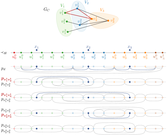
Figure 10: An instance $(G_{C},3,(V_{1},V_{2},V_{3}))$ of McC (top) and the SLE instance resulting from our construction (bottom). Colors indicate (correspondence to) the partition. The extension $\langle\prec,\sigma\rangle$ indicated in saturated colors induces the colorful 3-clique $\mathcal{C}=\{v_{1}^{1},v_{2}^{1},v_{3}^{1}\}$ in $G_{C}$. The edges in $G_{C}[\mathcal{C}]$ and their corresponding pages are highlighted in red.

Figure 10 shows an example of the reduction for a small graph $G_{C}$ with three colors. Taking a closer look at our construction for Theorem 6.4 (and Figure 10), we make the following observation. Consider a line $l$ perpendicular to the spine. On the page $p_{e}$ for an edge $e=v_{\alpha}^{i}v_{\beta}^{j}\in E(G_{C})$, the line $l$ intersects at most one edge if placed in the interval for a color $\gamma$ with $\gamma<\alpha$ or $\gamma>\beta$. If $\alpha<\gamma<\beta$, the line $l$ can in addition intersect the edges $u_{\alpha}^{i}u_{\beta}^{j+1}$ and $u_{\alpha}^{i+1}u_{\beta}^{j}$ of Figure 8c. Finally, if $\gamma\in\{\alpha,\beta\}$, the line $l$ intersects at most the full span of the tunnel, which has a width of three, see again Figure 8. Hence, the width of the page $p_{e}$ is at most three. Similarly, for the page $p_{d}$, Figures 5 and 9 show that its width is also at most three. Hence, the page width $\omega$ of $\langle\prec_{H},\sigma_{H}\rangle$ is constant and we obtain Corollary 6.5.

Corollary 6.5.

SLE parameterized by the number $\kappa$ of missing vertices and edges and the page width $\omega$ of the given layout, i.e., by $\kappa+\omega$, is [1]-hard.

7 Adding the Number of Pages as Parameter for SLE

In this section, we complete the landscape of Figure 2 by showing that SLE becomes fixed-parameter tractable once we add $\ell$ to the parameterization considered by Corollary 6.5, i.e., we show the following theorem.

Theorem 7.1.

Let $\mathcal{I}=\left(\ell,G,H,\langle\prec,\sigma\rangle\right)$ be an instance of SLE. We can find an $\ell$-page stack layout of $G$ that extends $\langle\prec,\sigma\rangle$ or report that none exists in $\mathcal{O}(\ell^{m_{\text{add}}}\cdot{n_{\text{add}}{}}!\cdot m_{\text{add}}{}^{n_{\text{add}}{}}\cdot\omega^{m_{\text{add}}{}}\cdot(n_{\text{add}}{}\cdot m_{\text{add}}{}\cdot\left|\mathcal{I}{}\right|))$ time.

We will make use of the following concepts. Consider a page $p$ of a stack layout $\langle\prec,\sigma\rangle$ of $G$ and recall that we can interpret it as a plane drawing of the graph $G^{\prime}$ with $V(G^{\prime})=V(G)$ and $E(G^{\prime})=\{e\in E(G)\mid\sigma(e)=p\}$ on a half-plane, where the edges are drawn as (circular) arcs. A face on the page $p$ in $\langle\prec,\sigma\rangle$ coincides with the notion of a face in the drawing (on the half-plane $p$) of $G^{\prime}$. This also includes the definition of the outer-face. See Figure 11 for a visualization of these and the following concepts and observe that we can identify every face, except the outer-face, by the unique edge $e=uv\in E(G)$ with $u\prec v$ and $\sigma(e)=p$ that bounds it from upwards.

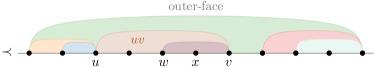
Figure 11: A stack layout $\langle\prec,\sigma\rangle$ and the faces on page $p$. Note that each edge has the same color as the face it identifies. While the vertex $w$ is incident to the face $uv$, the vertex $x$, and therefore also the interval $[w,x]$, is not. However, the face $uv$ still spans the interval $[w,x]$.

In the following, we will address a face by the edge it is identified with. Similarly, we say that an edge induces the face it identifies. We say that a vertex $w$ is incident to the face $uv$ (on some page $p$) if $u\preceq w\preceq v$ holds and there does not exist a different face $u^{\prime}v^{\prime}$ (on the page $p$) with $u\preceq u^{\prime}\preceq w\preceq v^{\prime}\preceq v$. Similarly, an interval $[w,x]$ is incident to a face if $w$ and $x$ are incident to the face. Finally, we say that a face $uv$ spans an interval $[w,x]$ if $u\preceq w\prec x\preceq v$ holds; note that $[w,x]$ might not be incident to the face $uv$.

Let $V_{\text{inc}}{}\subseteq V(H)$ be the vertices of $H$ that are incident to new edges, i.e., $V_{\text{inc}}{}\coloneqq\{u\in V(H)\mid\text{there is an edge}\ e=uv\in E_{\text{add}}{}\}$. The size of $V_{\text{inc}}$ is upper-bounded by $2m_{\text{add}}{}$. We will define an equivalence class on the intervals of $\prec_{H}$ based on the location of the vertices from $V_{\text{inc}}$. Consider the two intervals $[u_{1},v_{1}]$ and $[u_{2},v_{2}]$ defined by the old vertices $u_{1}$, $v_{1}$, $u_{2}$ and $v_{2}$, respectively. These two intervals are in the same equivalence class if and only if $\{w\in V_{\text{inc}}{}\mid w\preceq u_{1}\}=\{w\in V_{\text{inc}}{}\mid w\preceq u_{2}\}$ and $\{w\in V_{\text{inc}}{}\mid v_{1}\preceq w\}=\{w\in V_{\text{inc}}{}\mid v_{2}\preceq w\}$ holds.

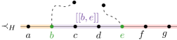
Figure 12: Visualization of super intervals. Each color represents one super interval. Vertices from $V_{\text{inc}}$ are marked in green.

Each equivalence class, which we call super interval, consists of a set of consecutive intervals delimited by (up to) two old vertices; see Figure 12. Note that the first and last super interval are defined by a single vertex $v\in V_{\text{inc}}{}$. The number of super intervals is bounded by $2m_{\text{add}}{}+1$. notationSuperIntervalWe denote the super interval delimited by the two vertices $u,v\in V_{\text{inc}}{}$ with $u\prec v$ by $[[u,v]]$. For the remainder of this paper, we assume that every super interval is bounded by two vertices. This is without loss of generality, since we can place dummy vertices at the beginning and end of the spine and assume that they bound the first and the last interval. Furthermore, we write $\curlyvee(w)=[[u,v]]$ to denote that the new vertex $w\in V_{\text{add}}{}$ is placed, with respect to a given spine order $\prec_{G}$, in the super interval $[[u,v]]$. Furthermore, for a given $\prec_{G}$, we define $\prec_{G\setminus H}$ to be its restriction to new vertices, i.e., for every two vertices $u,v\in V_{\text{add}}{}$ we have that $u\prec v$ implies $u\prec_{G\setminus H}{}v$.

A Helpful Lemma Towards the Fixed-Parameter Algorithm.

With the above concepts at hand, we can now describe our algorithm. It consists of a branching step, where we consider all possible page assignments for the new edges, all relative orders among the new vertices, all their possible assignment to super intervals, and all distances new edges can have from the outer-face. The core of our algorithm is a (dynamic programming) algorithm that we apply in each branch. In particular, we aim to show the following lemma.

Lemma 7.2.

Given an instance $\mathcal{I}=\left(\ell,G,H,\langle\prec,\sigma\rangle\right)$ of SLE, (i) a page assignment $\sigma_{G}$ for all edges, (ii) an order $\prec_{G\setminus H}$ in which the new vertices will appear along the spine, (iii) for every new vertex $v\in V_{\text{add}}{}$ an assignment to a super interval, and (iv) for every new edge $e$ an assigned distance $\omega_{e}$ to the outer face with respect to $H$ and $\langle\prec,\sigma\rangle$. In $\mathcal{O}(n_{\text{add}}{}\cdot m_{\text{add}}{}\cdot\left|\mathcal{I}{}\right|)$ time we can compute an $\ell$-page stack layout of $G$ that extends $\langle\prec,\sigma\rangle$ and respects the given assignments (i)–(iv) or report that no such layout exists.

We first observe that assignments (i)–(iv) fix everything except for the actual position of the new vertices within their super interval. Especially, assignment (i) allows us to check whether an edge $e\in E_{\text{add}}^{H}{}$ incident to two old vertices crosses any old edge or another new edge from $E_{\text{add}}^{H}{}$. Furthermore, assignments (i) and (ii) allow us to check whether two new edges $e=ua,e^{\prime}=vb\in E_{\text{add}}{}$ with $u,a,v,b\in V_{\text{add}}$ will cross. Adding assignment (iii), we can also check this for new edges with some endpoints in $V(H)$, i.e., extend this to all $u,a,v,b\in V(G)$. If the assignments imply a crossing or contradict each other, we can directly return that no desired layout exists. These checks can be performed in $\mathcal{O}({n_{\text{add}}{}}^{2}+m_{\text{add}}{}\cdot\left|\mathcal{I}{}\right|)$ time. It remains to check whether there exists a stack layout in which no edge of $E_{\text{add}}\setminus E_{\text{add}}^{H}$ intersects an old edge. This depends on the exact intervals new vertices are placed in.

To do so, we need to assign new vertices to faces such that adjacent new vertices are in the exact same face and not two different faces with the same distance to the outer face. We will find this assignment using a dynamic program that models whether there is a solution that places the first $j$ new vertices (according to $\prec_{G\setminus H}$) within the first $i$ intervals in $\prec_{H}$. When placing vertex $v_{j+1}$ in the $i$th interval, we check that all preceding neighbors are visible in the faces assigned by (iv). When advancing to the interval $i+1$, we observe that when we leave a face, all edges with the same or a higher distance to the outer face need to have both endpoints placed or none. We thus ensure that for no edge only one endpoint has been placed; see also Figure 13. These checks require $\mathcal{O}(m_{\text{add}}{})$ time for each of the $\mathcal{O}(n_{\text{add}}{}\cdot\left|V(H)\right|)$ combinations of $j$ and $i$. Once we reach the interval $\left|V(H)\right|+1$ and have successfully placed all $n_{\text{add}}$ new vertices, we know that there exists an $\ell$-page stack layout of $G$ that extends $\langle\prec,\sigma\rangle$ and respects the assignments. Finally, by applying standard backtracing techniques, we can extract the spine positions of the new vertices to also obtain the layout.

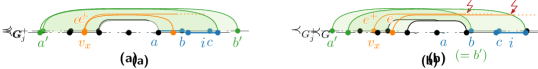
Figure 13: Illustration of advancing from the $i$th interval, marked in blue, to the interval $i+1$. In (a) and (b), we leave the green face and there exists an edge $e\in E_{\text{add}}$, marked in orange, with the same distance to the outer face as the green face. However, in (a), both end points of the edge $e$ have already been placed, whereas in (b) only one has, which implies a crossing.

sectionDP Before we show Lemma 7.2, we first make some observations on the assignments (i)–(iv) and their immediate consequences. In the following, we only consider consistent branches, i.e., we discard branches where from assignment (ii) we get $u\prec_{G\setminus H}{}v$ but from assignment (iii) $\curlyvee(u)=[[a,b]]$ and $\curlyvee(v)=[[c,d]]$ with $c\prec d\preceq a\prec b$, as this implies $v\prec u$.

First, we observe that assignment (i) fully determines the page assignment $\sigma_{G}$. Thus, it allows us to check whether an edge $e\in E_{\text{add}}^{H}{}$, i.e., a new edge incident to two old vertices, crosses any old edge or another new edge from $E_{\text{add}}^{H}{}$. From now on, we consider all edges from $E_{\text{add}}^{H}{}$ as old since their placement is completely determined by assignment (i).

Second, assignments (i) and (ii) allow us to check whether two new edges $e=ua,e^{\prime}=vb\in E_{\text{add}}{}$ with $u,a,v,b\in V_{\text{add}}$ will cross each other.

Third, adding assignment (iii), we can also check this for new edges with some endpoints in $V(H)$, i.e., extend this to all $u,a,v,b\in V(G)$. Hence, assignments (ii) and (iii) together with $\prec_{H}$ fix the relative order among vertices incident to new edges. Figure 14 shows an example where the assignments imply a crossings among two new edges.

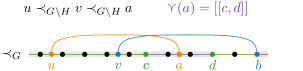
Figure 14: The crossing between the orange edge $e=ua$ and the blue edge $e^{\prime}=vb$, where the vertices $a$, $u$, and $v$ are new, is already implied by the page assignment $\sigma$ (assignment (i)), relative order among the new vertices $u$, $v$, and $a$, i.e., by $u\prec v\prec a$ (assignment (ii)), and their assignment to the super intervals, in particular by $\curlyvee(a)$ (assignment (iii)). The super intervals are indicated by color and we visualize one possible spine position of the new vertices consistent with the branch.

All of the above checks together can be done in $\mathcal{O}({n_{\text{add}}{}}^{2}+m_{\text{add}}{}\cdot\left|\mathcal{I}{}\right|)$ time. Clearly, if the assignments (i)–(iv) imply a crossing in an $\ell$-page stack layout of $G$ or contradict each other, we report that no layout exists that respects assignments (i)–(iv). However, if not, we still need to find concrete spine positions for the new vertices. The main challenge here is to assign new vertices to faces such that adjacent new vertices are in the same face and not two different faces with the same distance to the outer-face. For this, we use assignment (iv) together with the following dynamic programming (DP) algorithm.

The Intuition Behind the DP-Algorithm.

Recall that assignment (iv) determines for every new edge $e\in E_{\text{add}}{}$ the distance $\omega_{e}$ to the outer-face with respect to $\langle\prec_{H},\sigma_{H}\rangle$, i.e., how many edges of $H$ we need to remove until $e$ lies in the outer-face of the adapted stack layout $\langle\prec_{H},\sigma_{H}\rangle$; see also Figure 15.

Figure 15: Visualization of the semantics of $\omega_{e}$. Every face of $\langle\prec_{H},\sigma_{H}\rangle$ has one particular distance $\omega_{e}$ to the outer-face, shown in gray. Both highlighted new edges are in a face with $\omega_{e}=2$.

We first observe that $\omega_{e}$ together with $\sigma$ and the intervals in $\prec_{H}$ in which the endpoint vertices of $e$ are placed in uniquely determine a single face, namely the one the edge $e$ is embedded in. Furthermore, for every possible distance $\omega_{e}\in[\omega]_{0}$ and every interval in $\prec_{H}$, there is at most one face on page $\sigma(e)$ with distance $\omega_{e}$ to the outer-face that spans the interval. Hence, we address in the following for a given interval $[a,b]$ with $a\prec_{H}b$ the face on page $\sigma(e)$ at the distance $\omega_{e}$ to the outer-face, if it exists, with $\omega_{e}^{[a,b]}$. Note that $\omega_{e}^{[a,b]}=0$ always refers to the outer-face, independent of the vertices $a$ and $b$. However, for two different intervals $[a,b]$ and $[a^{\prime},b^{\prime}]$ the expressions $\omega_{e}^{[a,b]}$ and $\omega_{e}^{[a^{\prime},b^{\prime}]}$ can identify two different faces.

As a consequence of the above observation, we can decide for each interval of $\prec_{H}$ whether we can position a new vertex $v$ there, i.e., whether $v$ sees its adjacent vertices using the faces (in the assigned pages) at the corresponding distance from the outer-face. We now consider the ordering of the new vertices as in $\prec_{G\setminus H}$, i.e., we have $v_{1}\prec v_{2}\prec\ldots\prec v_{n_{\text{add}}{}}$. Furthermore, we number the intervals of $\prec_{H}$ from left to right and observe that there are $\left|V(H)\right|+1$ intervals.

Consider a hypothetical solution $\langle\prec,\sigma\rangle$ which we cut vertically at the $i$th interval of $\prec_{H}$. This partitions the new vertices into those that have been placed left and right of the cut. For new vertices placed in the $i$th interval of $\prec_{H}$, different cuts at the $i$th interval yield different partitions into left and right. Furthermore, some of the new edges lie completely on one side of the cut, while others span the cut. For $j\in[n_{\text{add}}{}]$, let $G_{j}$ be the graph $G[V(H)\cup\{v_{1},\ldots,v_{j}\}]$, i.e., the subgraph of $G$ induced by the vertices of $H$ and the first $j$ new vertices. We will refer to edges that span the cut and thereby only have one endpoint in $G_{j}$ as half-edges and denote with $v\cdot$ a half-edge with endpoint $v\in G_{j}$. Let $G_{j}^{+}$ be $G_{j}$ extended by the half-edges $E_{j}^{+}=\{v_{x}\cdot\mid v_{x}v_{y}\in E_{\text{add}}{},\ 1\leq x\leq j<y\leq n_{\text{add}}{}\}$; see Figure 16.

Figure 16: (a) The graph $G$ with the new vertices and edges highlighted in blue and (b) the graphs $G_{2}$ and (c) $G_{2}^{+}$. Half-edges are indicated with dashed lines.

In the following, we denote with $e^{+}$ the half-edge that we create for the edge $e$. For the half-edge $e^{+}=v_{x}\cdot$ and the edge $e=v_{x}v_{y}$, we call the vertex $v_{x}$ inside $G_{j}$, denoted as $V_{j}(e)$, and the vertex $v_{y}$ outside $G_{j}$, denoted as $\overline{V_{j}}(e)$.

Consider again the hypothetical solution $\langle\prec,\sigma\rangle$ and its vertical cut at the $i$th interval. Assume that $j$ vertices have been placed in $\langle\prec,\sigma\rangle$ left of the cut. The stack layout $\langle\prec,\sigma\rangle$ witnesses the existence of a stack layout for $G_{j}$ that extends $\langle\prec_{H},\sigma_{H}\rangle$ and uses only the first $i$ intervals. Furthermore, for every half-edge $e^{+}$ in $G_{j}^{+}$ the face where $e$ is placed in gives us a set of candidate intervals for the vertex $\overline{V_{j}}(e)$, namely those incident to that face. Hence, we can describe a partial solution of $\langle\prec,\sigma\rangle$ by a tuple $(i,j)$.

The DP-Algorithm.

Let $D$ be an $(\left|V(H)\right|+1)\times(n_{\text{add}}{}+1)\times 2$ binary table. In the following, we denote an entry $(i,j,r)$ for $i\in[\left|V(H)\right|+1]$, $j\in[n_{\text{add}}{}+1]$, and $r\in\{0,1\}$ as a state of the algorithm. A state $(i,j,r)$ for $i\in[\left|V(H)\right|+1]$, $j\in[n_{\text{add}}{}+1]$, and $r\in\{0,1\}$ is called feasible if and only if there exists, in the current branch, an extension of $\langle\prec_{H},\sigma_{H}\rangle$ for the graph $G_{j}$ with the following properties.

1. The $j$ new vertices are positioned in the first $i$ intervals and their placement respects assignment (iii).

2. If $r=1$, the last vertex $v_{j}$ has been placed in the $i$th interval. Otherwise, i.e., if $r=0$, the last vertex $v_{j}$ has been placed in some interval $i^{\prime}$ with $i^{\prime}<i$.

3. For every half-edge $e^{+}$ of $G_{j}^{+}$, the face in which we placed (the first endpoint of) $e^{+}$ spans the $i$th interval.

Note that for Item 3, we neither require that there exists some interval $i^{\prime}$ with $i\leq i^{\prime}$ for the vertex $\overline{V_{j}}(e)$ that is incident to $\omega_{e}^{i}$ nor that this $i^{\prime}$th interval is part of $\curlyvee(\overline{V_{j}}(e))$, i.e., the super interval for $\overline{V_{j}}(e)$ according to assignment (iii). However, we will ensure all of the above points in the DP when placing $\overline{V_{j}}(e)$. Furthermore, while the last (binary) dimension is technically not necessary, it simplifies our following description. Finally, note that we (correctly, as required in some solutions) allow to position multiple vertices in the same interval of $\prec_{H}$.

Our DP will mark a state $(i,j,r)$ for $i\in[\left|V(H)\right|+1]$, $j\in[n_{\text{add}}{}+1]$, and $r\in\{0,1\}$ as feasible by setting $D[i,j,r]=1$. Before we can show in Lemma 7.4 that our DP indeed captures this equivalence, let us first relate different states and thus also partial solutions to each other. We observe that if we have a solution for $i\in[\left|V(H)\right|]$, $j\in[n_{\text{add}}{}]_{0}$, and $r\in\{0,1\}$, and for every half-edge $e^{+}$ of $G_{j}^{+}$ the face $\omega_{e}^{i}$ also spans the $i+1$th interval, then we also have a solution in the state $(i+1,j,0)$. Otherwise, we cannot find an interval for the vertex $\overline{V_{j}}(e)$ for some half-edge $e^{+}$ of $G_{j}^{+}$; see Figure 17b.

Figure 17: Illustration of some partial solution $(i,j)$ with the half-edge $e^{+}=v_{x}\cdot$ in $G_{j}^{+}$ that we place in the green face. The $i$th interval is $[a,b]$, highlighted in blue, and $\omega_{e}^{i}$ is identified by the green edge $a^{\prime}b^{\prime}$. In (a), the partial solution $(i,j,r)$ is an admissible predecessor of $(i+1,j,0)$, whereas in (b) it is not as we can no longer find an interval for the vertex $\overline{V_{j}}(e)$ that does not introduce a crossing between $e$ and $a^{\prime}b^{\prime}$. In particular, observe that the face $\omega_{e}^{i}$ does not span the interval $[b,c]$.

More formally, let $[a,b]$ be the $i$th interval and $[b,c]$ the $i+1$th interval. Assume that we have the new edge $e=v_{x}v_{y}$ in $G$ with $1\leq x\leq j<y\leq k$, which is the half-edge $v_{x}\cdot$ in $G_{j}^{+}$. Let $a^{\prime}b^{\prime}$ be the edge (on page $\sigma_{G}(e)$) that bounds the face identified by $\omega_{e}^{i}$ upwards with $a^{\prime}\prec b\preceq b^{\prime}$. We call $(i,j,r)$ an admissible predecessor of $(i+1,j,0)$ if $b\neq b^{\prime}$; see Figure 17a.

If we decide to place the vertex $v_{j}$ in the $i$th interval, say $[a,b]$, we have to be more careful. In particular, we have to ensure the following criteria before we can conclude that $(i,j,1)$ has an extension.

1. The interval $[a,b]$ is part of the super interval $\curlyvee(v_{j})$, i.e., we place the new vertex in the determined super interval.

2. For all new edges $e=v_{j}u$ with $u\in V(H)$ the face $\omega_{e}^{i}$ exists on the page $\sigma_{G}(e)$ and both the interval $i$ (and thus $v_{j}$) and $u$ are incident to the face $\omega_{e}^{i}$.

3. For all new edges $e=v_{j}v_{q}$ incident to two new vertices the face $\omega_{e}^{i}$ exists on the page $\sigma_{G}(e)$ and the interval $i$ (and thus $v_{j}$) is incident to it.

The second criterion ensures that edges incident to $v_{j}$ and an old vertex can be inserted without introducing a crossing. The third criterion ensures for a new edge $e$ incident to two new vertices that the half-edge $e^{+}$ has been completed to a full edge without introducing a crossing or is placed in the face $\omega_{e}^{i}$ that spans the $i$th interval (if $j<q$). Similar to before, we call $(i,j-1,r)$ an admissible predecessor of $(i,j,1)$ if all of the above criteria are met. Finally, note that if we decide to place the vertex $v_{j}$ in the $i$th interval, then the state $(i,j,0)$ is not feasible due to Item 2. Our considerations up to now are summarized by the recurrence relation in Definition 7.3. In Lemma 7.4, we show that the recurrence relation identifies exactly all feasible states and thus partial solutions.

Definition 7.3.

We have the following relation for all $i\in[2,\left|V(H)\right|+1]$ and $j\in[n_{\text{add}}{}]_{0}$.

$$D[1,0,0] =1$$ (2)

$$D[1,0,1] =0$$ (3)

$$D[i,j,0] =\begin{cases}1&\ \text{if}\ (i-1,j,r)\ \text{is an admissible predecessor of}\ (i,j,0)\\ &\ \text{and}\ D[i-1,j,r]=1\ \text{for some}\ r\in\{0,1\}\\ 0&\ \text{otherwise}\end{cases}$$ (4)

$$D[i,j,1] =\begin{cases}1&\ \text{if}\ (i,j-1,r)\ \text{is an admissible predecessor of}\ (i,j,1)\\ &\ \text{and}\ D[i,j-1,r]=1\ \text{for some}\ r\in\{0,1\}\\ 0&\ \text{otherwise}\end{cases}$$ (5)

Lemma 7.4.

For all $i\in[\left|V(H)\right|+1]$, $j\in[n_{\text{add}}{}]_{0}$, and $r\in\{0,1\}$ we have $D[i,j,r]=1$ if and only if the state $(i,j,r)$ is feasible. Furthermore, evaluating the recurrence relation of Definition 7.3 takes $\mathcal{O}(m_{\text{add}}{})$ time.

Proof 7.5.

We first use induction over $i$ and $j$ to show correctness of the recurrence relation and later argue the time required to evaluate it. In the following, we let $[a,b]$ be the $i$th interval.

*Base Case ($\boldsymbol{i=1}$ and $\boldsymbol{j=0}$). If we have $i=1$ and $j=0$, we are in the first interval and have not placed any new vertex. Thus, $G_{j}=G_{j}^{+}=H$ holds and $G_{j}$ has clearly a solution, namely $\langle\prec_{H},\sigma_{H}\rangle$. Furthermore, there are no half-edges in $G_{j}^{+}$ and thus $(1,0,r)$ is a feasible state if and only if $r=0$. Note that $(1,0,1)$ contradicts Item 2 and thus cannot be a feasible state. Hence, Equations 2 and 3 are correct and serve as our base case.

In our inductive hypothesis, we assume that the table $D$ has been correctly filled up until some value $i^{\prime}\in[\left|V(H)\right|+1]$ and $j^{\prime}\in[n_{\text{add}}{}]_{0}$.

*Inductive Step for $\boldsymbol{i}$ ($\boldsymbol{i=i^{\prime}+1}$ and $\boldsymbol{j=j^{\prime}}$). First, note that by moving one interval to the right, having $r=1$ is not possible and hence we focus on Equation 4 in this step. We consider the cases $D[i,j,0]=1$ and $D[i,j,0]=0$ separately.

For $D[i,j,0]=1$, there exists by the definition of Equation 4 an admissible predecessor $(i^{\prime},j,r)$ for some $r\in\{0,1\}$ with $D[i^{\prime},j,r]=1$. By our inductive hypothesis, this means that the state $(i^{\prime},j,r)$ is feasible. In particular, it has a solution for $G_{j}$ that places all new vertices in the first $i^{\prime}$ intervals. Clearly, the same solution positions them also in the first $i$ intervals. Furthermore, every half-edge $e^{+}$ of $G_{j}^{+}$ is assigned to a face that spans the $i^{\prime}$th interval. As $(i^{\prime},j,r)$ is an admissible predecessor, we know that for every $e\in G_{j}^{+}$ the face $\omega_{e}^{i^{\prime}}$ also spans the $i$th interval. Hence, the state $(i,j,0)$ is feasible, i.e., $D[i,j,0]=1$ correctly holds.

For $D[i,j,0]=0$, there are two cases to consider by the definition of Equation 4. Either $(i,j,0)$ does not have an admissible predecessor, or for all admissible predecessors $(i^{\prime},j,r)$ of $(i,j,0)$ we have $D[i^{\prime},j,r]=0$. Observe that only states of the form $(i^{\prime},j,r)$ for some $r\in\{0,1\}$ can be admissible predecessors. In the former case, there exists by our definition of admissible predecessor some half-edge $e^{+}$ in $G_{j}^{+}$ that is assigned to the face $\omega_{e}^{i^{\prime}}$ which does not span the $i$th interval. Hence, $(i,j,0)$ is not feasible by Item 3. In the latter case, we know by our inductive hypothesis that $D[i^{\prime},j,r]=0$ implies that $(i^{\prime},j,r)$ is not feasible, i.e., there does not exist a solution for the graph $G_{j}$ in which we place the new vertices in the first $i^{\prime}$ intervals. As we do not place the vertex $v_{j}$ in the $i$th interval, no solution can exist for the state $(i,j,0)$ either and $D[i,j,0]=0$ correctly holds. This concludes the inductive step for $i$.

*Inductive Step for $\boldsymbol{j}$ ($\boldsymbol{i=i^{\prime}}$ and $\boldsymbol{j=j^{\prime}+1}$). Analogous to before, we note that by placing $v_{j}$ in the $i$th interval, $r=0$ is not possible and hence we focus on Equation 5 in this step. We again consider the cases $D[i,j,1]=1$ and $D[i,j,1]=0$ separately.

For $D[i,j,1]=1$, there exists an admissible predecessor $(i,j^{\prime},r)$ for some $r\in\{0,1\}$ with $D[i,j^{\prime},r]=1$ by the definition of Equation 5. By our inductive hypothesis, this means that the state $(i,j^{\prime},r)$ is feasible and has a solution $\langle\prec_{G_{j-1}},\sigma_{G_{j-1}}\rangle$ that places all new vertices of $G_{j-1}$ in the first $i$ intervals. We now construct a solution $\langle\prec_{G_{j}},\sigma_{G_{j}}\rangle$ by setting $\sigma_{G_{j}}$ according to assignment (i), and extending the spine order $\prec_{G_{j-1}}$ by placing $v_{j}$ in the $i$th interval. More concretely, we take $\prec_{G_{j-1}}$, set $a\prec v_{j}\prec b$, and take the transitive closure to obtain a linear order on the vertices of $G_{j}$. As $(i,j^{\prime},r)$ is an admissible predecessor, $v_{j}$ is placed within $\curlyvee(v_{j})$ in $\langle\prec_{G_{j}},\sigma_{G_{j}}\rangle$ and $\langle\prec_{G_{j}},\sigma_{G_{j}}\rangle$ extends $\langle\prec_{H},\sigma_{H}\rangle$. So it remains to show that $\langle\prec_{G_{j}},\sigma_{G_{j}}\rangle$ is crossing-free. As we discard all assignments (i)–(iv) that imply a crossing among two new edges, a new edge $e$ incident to $v_{j}$ could only cross an old edge $e^{\prime}$. However, as $(i,j^{\prime},r)$ is an admissible predecessor, we have that the vertices incident to $e$ lie in the same face $\omega_{e}^{i}$. Every old edge induces a face of $\langle\prec_{H},\sigma_{H}\rangle$. Therefore, we deduce that a crossing between an old and a new edge whose endpoints lie in the same face is impossible. Consequently, also $e$ and $e^{\prime}$ cannot cross. Thus, $\langle\prec_{G_{j}},\sigma_{G_{j}}\rangle$ is a solution for the graph $G_{j}$. Finally, it is clear that for every half-edge $e^{+}$ of $G_{j}^{+}$, the face assigned to its associated edge $e$ spans the $i$th interval. For half-edges that already existed in $G_{j^{\prime}}^{+}$, this holds as $(i,j^{\prime},r)$ is feasible. For half-edges introduced in $G_{j}^{+}$, this holds by the definition of admissible predecessor; see Items 2 and 3. Thus, $(i,j,1)$ is feasible and $D[i,j,1]=1$ correctly holds.

For $D[i,j,1]=0$, there are again two cases to consider by the definition of Equation 5. Either $(i,j,1)$ does not have an admissible predecessor, or for all admissible predecessors $(i,j^{\prime},r)$ of $(i,j,0)$ we have $D[i,j^{\prime},r]=0$. Again, we observe that it suffices to consider only states of the form $(i,j^{\prime},r)$ for some $r\in\{0,1\}$ as potential admissible predecessors. For the former case, clearly, if both such states $(i,j^{\prime},r)$ are not admissible predecessors, then $(i,j,1)$ cannot be feasible: Either, we violate Item 1 by placing $v_{j}$ outside $\curlyvee(v_{j})$, which contradicts assignment (iii), or an edge $e$ incident to $v_{j}$ crosses an old edge as one of its endpoints is not incident to $\omega_{e}^{i}$; see Items 2 and 3. Note that we can assume that all relevant faces span the $i$th interval, as we have already shown that the inductive step for $i$ is correct. In both cases, $(i,j,1)$ is clearly not feasible; see Item 1 for the former and observe that a crossing contradicts the existence of an extension for the latter case. We now consider the case where all admissible predecessor $(i,j^{\prime},r)$ of $(i,j,1)$ have $D[i,j^{\prime},r]=0$. Using proof by contradiction, we show that in this case $(i,j,1)$ cannot be feasible either. Assume that $(i,j,1)$ would be a feasible state. Then, there exists a solution $\langle\prec_{G_{j}},\sigma_{G_{j}}\rangle$ for the graph $G_{j}$. Using $\langle\prec_{G_{j}},\sigma_{G_{j}}\rangle$, we can create a solution $\langle\prec_{G_{j^{\prime}}},\sigma_{G_{j^{\prime}}}\rangle$ for $G_{j^{\prime}}$ by removing $v_{j}$ from $\prec_{G_{j}}$ and all its incident edges from $\sigma_{G_{j}}$. Clearly, $\langle\prec_{G_{j^{\prime}}},\sigma_{G_{j^{\prime}}}\rangle$ respects the assignments (i)–(iv). Furthermore, for every half-edge $e^{+}$ in $G_{j}^{+}$, the assigned face spans the $i$th interval as $(i,j,1)$ is feasible; see Item 3. For every half-edge $e^{+}$ in $G_{j^{\prime}}^{+}$ with $\overline{V_{j^{\prime}}}(e)=v_{j}$, i.e., that was completed to an ordinary edge in $G_{j}$, the assigned face spans the $i$th interval as it is incident to it. Hence, if $(i,j,1)$ is feasible and $(i,j^{\prime},r)$ is an admissible predecessor, then $(i,j^{\prime},r)$ is also feasible. However, this contradicts the inductive hypothesis, as we have $D[i,j-1,r]=0$. Thus, the state $(i,j,1)$ cannot be feasible and $D[i,j,1]=0$ correctly holds. This concludes the inductive step for $j$.

*Evaluation Time of Recurrence Relation. We observe that, apart from checking whether a state is an admissible predecessor of $(i,j,r)$, the steps required to perform in order to evaluate the recurrence relation take constant time. In the following, we assume that we can access a look-up table that stores the faces in $\langle\prec_{H},\sigma_{H}\rangle$ that span a given interval in $\prec_{H}$ on a given page $p\in[\ell]$ ordered from outside in, i.e., starting with the outer-face. We will account for this in our proof of Lemma 7.2. In Equation 4, we ensure for every half-edge $e^{+}$ in $G_{j}^{+}$ that the face $\omega_{e}^{i-1}$ does not end at the interval $i-1$. As there are at most $m_{\text{add}}$ half-edges, we can do this in $\mathcal{O}(m_{\text{add}}{})$ time. For Equation 5, we have to ensure that the $i$th interval $[a,b]$ is part of $\curlyvee(v_{j})$, which takes constant time. Furthermore, we have to check for every new edge $e=v_{j}u$ that the face $\omega_{e}^{i}$ exists on the page $\sigma(e)$ and that $v_{j}$ is incident to it. For a single edge, this takes constant time, as we can look up the faces that span the $i$th interval and $v_{j}$ is always incident to the bottom-most face. Furthermore, if $u\in V(H)$ holds, we also have to check if $u$ is incident to $\omega_{e}^{i}$. If $u\preceq a\prec b$, we can access the faces that span the interval $[u,\text{succ}(\prec_{H},\ u)]$ and check if $u$ is incident to the face $\omega_{e}^{i}$. An analogous check can be made if we have $a\prec b\preceq u$. This takes constant time per edge $e$. Hence, we can evaluate Equation 5 in $\mathcal{O}(m_{\text{add}}{})$ time. Combining all, the claimed running time follows.

Putting Everything Together.

With our DP at hand, we are now ready to prove Lemma 7.2.

Proof 7.6 (Proof of Lemma 7.2.).

First, recall that we can check in $\mathcal{O}({n_{\text{add}}{}}^{2}+m_{\text{add}}{}\cdot\left|\mathcal{I}{}\right|)$ time whether assignments (i)–(iv) are consistent and do not imply a crossing. Thus, we assume for the remainder of the proof that they are. Furthermore, recall that there are $\left|V(H)\right|+1$ intervals in $\langle\prec_{H},\sigma_{H}\rangle$ and observe that we have $G_{k}=G_{k}^{+}=G$. Therefore, $G_{k}^{+}$ does not not contain any half-edge and the feasibility propery Item 3 is trivially satisfied. Hence, as a consequence of Lemma 7.4, we deduce that there exists an $\ell$-page stack layout of $G$ that extends $\langle\prec,\sigma\rangle$ and respects assignments (i)–(iv) if and only if $D[\left|V(H)\right|+1,n_{\text{add}}{},r]=1$ for $r=0$ or $r=1$. Furthermore, by applying standard backtracing techniques, we can also determine the concrete spine positions for every new vertex, i.e., compute such a stack layout.

We now bound the running time of the DP. For that, we first observe that the DP-table $D$ has $\mathcal{O}(n_{\text{add}}{}\cdot\left|V(H)\right|)$ entries. We have seen in Lemma 7.4 that the time required to evaluate the recurrence relation is in $\mathcal{O}(m_{\text{add}}{})$. However, we assumed that we have access to a lookup-table that stores for each interval and each page the faces that span it. We can compute this table in a pre-processing step by iterating from left to right over the spine order $\prec_{H}$ and keeping at each interval $[a,b]$ for each page $p$ track of the edges $a^{\prime}b^{\prime}$ with $\sigma(a^{\prime}b^{\prime})=p$ and $a^{\prime}\preceq a\prec b\preceq b$. This can be done in $\mathcal{O}(\left|\mathcal{I}{}\right|^{2})$ time. However, as this table can be re-used in different invocations of the DP-Algorithm, it has to be computed only once in the beginning. As the overall running time of the -algorithm will clearly dominate $\mathcal{O}(\left|\mathcal{I}{}\right|^{2})$, we neglect this pre-computation step. Hence, the running time of the DP is $\mathcal{O}(n_{\text{add}}{}\cdot\left|V(H)\right|\cdot m_{\text{add}}{})$ and together with the initial checks, this amounts to $\mathcal{O}(n_{\text{add}}{}\cdot m_{\text{add}}{}\cdot\left|\mathcal{I}{}\right|)$ time.

Finally, we observe that for assignment (i), i.e., $\sigma_{G}$, there are $\mathcal{O}(\ell^{m_{\text{add}}})$ different possibilities, for assignment (ii), i.e., $\prec_{G\setminus H}$, there are $\mathcal{O}({n_{\text{add}}{}}!)$ possibilities, for assignment (iii), i.e., the assignment of new vertices to super intervals, there are $\mathcal{O}(m_{\text{add}}{}^{n_{\text{add}}{}})$ possibilities, and for assignment (iv), i.e., the distance to the outer face, there are $\mathcal{O}(\omega^{m_{\text{add}}{}})$ different possibilities. This gives us overall $\mathcal{O}(\ell^{m_{\text{add}}}\cdot{n_{\text{add}}{}}!\cdot m_{\text{add}}{}^{n_{\text{add}}{}}\cdot\omega^{m_{\text{add}}{}})$ different possibilities for assignments (i)–(iv). Applying Lemma 7.2 to each of these, we get the desired theorem:See 7.1

8 Towards a Tighter Fixed-Parameter Algorithm for SLE

As a natural next step, we would like to generalize Theorem 7.1 by considering only $\kappa$ and $\ell$ as parameters. However, the question of whether one can still achieve fixed-parameter tractability for SLE when parameterizing by $\kappa+\ell$ is still open. Nevertheless, as our final result, we show that strengthening Theorem 7.1 is indeed possible at least in the restricted case where no two missing vertices are adjacent, as we can then greedily assign the first “possible” interval to each vertex that complies with assignment (i)–(iii).

Theorem 8.1.

Let $\mathcal{I}=\left(\ell,G,H,\langle\prec,\sigma\rangle\right)$ be an instance of SLE where $G[V_{\text{add}}{}]$ is an independent set. We can find an $\ell$-page stack layout of $G$ that extends $\langle\prec,\sigma\rangle$ or report that none exists in $\mathcal{O}(\ell^{m_{\text{add}}{}}\cdot n_{\text{add}}{}!\cdot{m_{\text{add}}{}}^{n_{\text{add}}{}}\cdot(m_{\text{add}}{}{\left|\mathcal{I}{}\right|}^{2}))$ time.

ptheoremIndependentSetFPT Observe that $G[V_{\text{add}}{}]$ being an independent set removes the need for synchronizing the position of adjacent new vertices to ensure that they are incident to the same face. We propose a fixed-parameter algorithm that loosely follows the ideas introduced in Section 7 and adapts them to the considered setting. The following claim will become useful. Given an instance $\mathcal{I}=\left(\ell,G,H,\langle\prec,\sigma\rangle\right)$ of SLE where $G[V_{\text{add}}{}]$ is an independent set, (i) a page assignment $\sigma_{G}$ for all edges, (ii) an order $\prec_{G\setminus H}$ in which the new vertices will appear along the spine, and (iii) for every new vertex $v\in V_{\text{add}}{}$ an assignment to a super interval. In $\mathcal{O}(m_{\text{add}}{}\cdot{\left|\mathcal{I}{}\right|}^{2})$ time we can compute an $\ell$-page stack layout of $G$ that extends $\langle\prec,\sigma\rangle$ and respects the given assignments (i)–(iii) or report that no such layout exists. Towards showing the claim, we first note that we only miss assignment (iv) from Lemma 7.2. Hence, by the same arguments as in the proof of Lemma 7.2, we can check in $\mathcal{O}({n_{\text{add}}{}}^{2}+m_{\text{add}}{}\cdot\left|\mathcal{I}{}\right|)$ time whether assignments (i)–(iii) are consistent and do not imply a crossing. For the remainder of the proof, we assume that they are, as we can otherwise immediately return that there does not exist an $\ell$-page stack layout of $G$ that respects the assignments.

We still need to to assign concrete spine positions to new vertices. However, in contrast to Theorem 7.1, there is no need to ensure that adjacent new vertices are in the same face, because there are no two new vertices are adjacent by assumption. This allows us to use a greedy variant of the DP from Theorem 7.1.

The Greedy Algorithm. We maintain a counter $j$ initialized at $j=1$ and consider the $i$th interval $[a,b]$. If $[a,b]\in\curlyvee(v_{j})$, i.e., if $[a,b]$ is part of the super interval for $v_{j}$, we check the following for every new edge $e=v_{j}u\in E_{\text{add}}{}$ incident to $v_{j}$. Assuming that $v_{j}$ would be placed in $[a,b]$, we check whether $v_{j}$ sees $u$ on the page $\sigma(e)$. These checks can be done in $\mathcal{O}(m_{\text{add}}{}\cdot\left|\mathcal{I}{}\right|)$ time. If this is the case, we place $v_{j}$ in the interval $[a,b]$ and increase the counter by one, otherwise we continue with the next interval $[b,c]$. We stop once we have $j=k+1$ as we have assigned an interval to all new vertices. To obtain the $\ell$-page stack layout of $G$, we can store in addition for each vertex the interval we have placed it in. If after processing the last interval there are still some new vertices that have not been placed, we can return that there does not exist an $\ell$-page stack layout of $G$ that extends $\langle\prec_{H},\sigma_{H}\rangle$ and respects the assignments (i)—(iii). The greedy algorithm runs in $\mathcal{O}(m_{\text{add}}{}\cdot{\left|\mathcal{I}{}\right|}^{2})$ time.

Correctness of the Greedy Algorithm. In the following, we show that if there is an $\ell$-page stack layout of $G$ that extends $\langle\prec_{H},\sigma_{H}\rangle$ and respects assignments (i)–(iii), then our greedy algorithm finds also some. To that end, we assume that there is such a stack layout $\langle\prec^{*}_{G},\sigma^{*}_{G}\rangle$. As we only assign intervals and thus spine positions to the new vertices, it suffices to show that if $\langle\prec^{*}_{G},\sigma^{*}_{G}\rangle$ is a solution, so is $\langle\prec,\sigma^{*}_{G}\rangle$, where $\prec$ is the spine order we obtain with our greedy algorithm. Observe that we must find some tuple $\langle\prec_{G},\sigma_{G}\rangle$ that extends $\langle\prec_{H},\sigma_{H}\rangle$ and respects the assignments (i)–(iii), as we only ensure that no new edge incident to a new vertex crosses old edges. As this is clearly not the case in $\langle\prec^{*}_{G},\sigma^{*}_{G}\rangle$, there must be a feasible interval for each new vertex. For the remainder of the proof, we assume that $\prec^{*}_{G}$ and $\prec$ differ only in the position of some new vertex $v$. This is without loss of generality, as we can apply the following arguments for all new vertices iteratively from left to right according to $\prec^{*}_{G}$, until all of them are placed as in the greedy solution. As we assign the intervals greedily, we assume that $v\prec^{*}_{G}u$ implies $v\prec u$ for all old vertices $u$, i.e., $v$ appears in $\prec$ earlier than in $\prec^{*}_{G}$. Clearly, $\langle\prec,\sigma^{*}_{G}\rangle$ extends $\langle\prec_{H},\sigma_{H}\rangle$ as $\langle\prec^{*}_{G},\sigma^{*}_{G}\rangle$ does. Therefore, we only need to show that $\langle\prec,\sigma^{*}_{G}\rangle$ does not contain crossings.

Towards a contradiction, assume that $\langle\prec,\sigma^{*}_{G}\rangle$ contains a crossing among the edges $e=vu$ and $e^{\prime}=ab$. We assume that $e$ is a new edge incident to the new vertex $v$ and observe that $u$ must be an old vertex. Furthermore, we assume without loss of generality that $b$ is also an old vertex. As already argued in the beginning, we have checked, when placing $v$, that $e$ does not cross an old edge. Hence, we observe that $e^{\prime}$ cannot be an old edge. As we also treated all new edges incident to two old vertices as old edges, we conclude that $e^{\prime}$ must be a new edge incident to a new vertex $a$ and an old vertex $b$. Furthermore, we assume $a\prec^{*}_{G}b$, $a\prec^{*}_{G}v$, and $v\prec^{*}_{G}u$. This is without loss of generality, as in any other case the arguments will be symmetric. As $\langle\prec^{*}_{G},\sigma^{*}_{G}\rangle$ is crossing free, we have $a\prec^{*}_{G}b\prec^{*}_{G}v\prec^{*}_{G}u$ or $a\prec^{*}_{G}v\prec^{*}_{G}u\prec^{*}_{G}b$. Furthermore, as our greedy algorithm positions $v$ further to the left compared to $\prec^{*}_{G}$ and $e$ and $e^{\prime}$ now cross, we must have $a\prec v\prec b\prec u$ or $v\prec a\prec u\prec b$, respectively. However, we observe that neither situation is possible.

For the former case, i.e., when we turn $a\prec^{*}_{G}b\prec^{*}_{G}v\prec^{*}_{G}u$ into $a\prec v\prec b\prec u$, we observe that $b$ is an old vertex incident to a new edge, i.e., it defines a super interval, see also Figure 18a. Hence, having $b\prec^{*}_{G}v$ and $v\prec b$ implies that the super interval for $v$ differs between $\langle\prec^{*}_{G},\sigma^{*}_{G}\rangle$ and $\langle\prec,\sigma^{*}_{G}\rangle$, which violates assignment (iii) and thus contradicts our assumption on the existence of $\langle\prec^{*}_{G},\sigma^{*}_{G}\rangle$ and $\langle\prec_{G},\sigma^{*}_{G}\rangle$.

In the latter case, when we turn $a\prec^{*}_{G}v\prec^{*}_{G}u\prec^{*}_{G}b$ into $v\prec a\prec u\prec b$, we move $v$ left of the new vertex $a$. Hence, we change the relative order among the new vertices, see Figure 18b. This is a contradiction to assignment (ii) and thus our assumption on the existence of $\langle\prec^{*}_{G},\sigma^{*}_{G}\rangle$ and $\langle\prec_{G},\sigma^{*}_{G}\rangle$.

As we obtain in all cases a contradiction, we conclude that $e$ and $e^{\prime}$ cannot cross. Applying the above arguments inductively, we derive that our algorithm must find a solution if there exists one, i.e., is correct.

*Putting Everything Together. We can now branch over all possible assignments (i)—(iii). For assignment (i), i.e., $\sigma_{G}$, there are $\mathcal{O}(\ell^{m_{\text{add}}})$ different possibilities, for assignment (ii), i.e., $\prec_{G\setminus H}$, there are $\mathcal{O}({n_{\text{add}}{}}!)$ possibilities, and for assignment (iii), i.e., the assignment of new vertices to super intervals, there are $\mathcal{O}(m_{\text{add}}{}^{n_{\text{add}}{}})$ possibilities This gives us overall $\mathcal{O}(\ell^{m_{\text{add}}}\cdot{n_{\text{add}}{}}!\cdot m_{\text{add}}{}^{n_{\text{add}}{}})$ different possibilities for assignments (i)–(iii). Applying our greedy algorithm to each of them, we obtain the theorem. figFPTISCorrectness

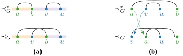
Figure 18: Illustration of the correctness arguments in the proof of Theorem 8.1. In (a), we change the assignment of $v$ to super intervals, highlighted with the colors, and in (b), we change the relative order among the new vertices $a$ and $v$. Both scenarios lead to a contradiction.

9 Concluding Remarks

Our results provide the first investigation of the drawing extension problem for stack layouts through the lens of parameterized algorithmics. We show that the complexity-theoretic behavior of the problem is surprisingly rich and differs from that of previously studied drawing extension problems. One prominent question left for future work is whether one can still achieve fixed-parameter tractability for SLE when parameterizing by $\kappa+\ell$, thus generalizing Theorem 7.1 and Theorem 8.1. A further natural and promising direction for future work is to consider generalizing the presented techniques to other types of linear layouts, such as queue layouts. Finally, future work could also investigate the following generalized notion of extending linear layouts: Given a graph $G$, the spine order for some subset of its vertices and the page assignment for some subset of its edges, does there exist a linear layout of $G$ that extends both simultaneously?

Appendix A Removing Multi-Edges

In the following section, we will describe how one can adapt the - and [1]-hardness reductions to not rely on multi-edges. While the basic idea is always the same, namely to introduce several auxiliary vertices in order to distribute the multiple edges among them, the concrete implementation depends on the (part of) the reduction we are currently discussing, see the following sections.

A.1 Fixation Gadget (Section 4.2)

While the fixation gadget gives us a lot of power to show hardness of different parameter combinations, we use multi-edges to construct it. As our graphs $H$ and $G$ are assumed to be simple, it is now time to remove these multi-edges by distributing them over several (additional) auxiliary vertices.

In order to do that, we no longer introduce the $2(F+1)$-many vertices $b_{1},\ldots,b_{F+1}$ and $a_{1},\ldots,a_{F+1}$, but introduce for each page $p\neq p_{d}$ $2(F+1)$ vertices $b_{1}^{p},\ldots,b_{F+1}^{p}$ and $a_{1}^{p},\ldots,a_{F+1}^{p}$. We also adapt the spine order $\prec_{H}$ and set $b_{i}^{p}\prec v_{i}\prec a_{i}^{p}$ for $i\in[F+1]$ and $p\in[\ell]\setminus\{p_{d}\}$. Furthermore, we fix the order among the newly introduced vertices by enforcing $b_{i}^{p+1}\prec b_{i}^{p}$ and $a_{i}^{p}\prec a_{i}^{p+1}$ for every $i\in[F+1]$ and $p\in[\ell]\setminus\{p_{d}\}$. The linear order $\prec$ is then obtained by taking the transitive closure of the above (partial) orders. Observe that the above spine order places for each page $p$ one vertex before ($b_{i}^{p}$) and after ($a_{i}^{i}$) $v_{i}$.

Next, we adapt the edges that we created in Section 4.2 and their page assignment $\sigma_{H}$. To that extend, recall that we introduced for every $i\in[F+1]$ and every page $p\neq p_{d}$ the edge $e(b_{i},a_{i},p)=b_{i}a_{i}$ with $\sigma(e(b_{i},a_{i},p))=p$. Now, this edge should be incident to vertices created “for the page $p$”, i.e., we create instead the edge $b_{i}^{p}a_{i}^{p}$ and set $\sigma(b_{i}^{p}a_{i}^{p})=p$. Although the remaining edges created in Section 4.2 are already simple, we have to adapt (some of) them, as their incident vertices no longer exist, i.e., have been replaced. In particular, for every $i\in[F+1]$, we now no longer introduce the edges $b_{i}v_{i}$ and $v_{i}a_{i}$ but the edges $b_{i}^{\ell-1}v_{i}$ and $v_{i}a_{i}^{\ell-1}$ and set $\sigma(b_{i}^{\ell-1}v_{i})=\sigma(v_{i}a_{i}^{\ell-1})=p_{d}$. Finally, we create instead of the edge $b_{1}a_{F+1}$ the edge $b_{1}^{\ell-1}a_{F+1}^{\ell-1}$ and set $\sigma(b_{1}^{\ell-1}a_{F+1}^{\ell-1})=p_{d}$. Figure 19 is an adapted version of Figure 5 and shows the updated construction.

Figure 19: An example for an adapted fixation gadget for $F=2$ with five other pages. Adapted version of Figure 5 that shows how we can remove multi-edges by distributing them over additional vertices.

We end this section with showing Lemma A.1, which is an adapted version of Lemma 4.1.

Lemma A.1.

Let $\mathcal{I}=\left(\ell,G,H,\langle\prec,\sigma\rangle\right)$ be an instance of SLE that contains the adapted fixation gadget (without multi-edges) on $F$ vertices $\{f_{1},\ldots,f_{F}\}$. In any solution $\langle\prec_{G},\sigma_{G}\rangle$ to $\mathcal{I}$ and for every $i\in[F]$, we have $v_{i}\prec f_{i}\prec v_{i+1}$ and $\sigma(f_{i}v_{i})=\sigma(f_{i}v_{i+1})=p_{d}$. Furthermore, the adapted fixation gadget contributes $2F\ell+2\ell-1$ vertices and $(\ell+4)F+\ell+2$ edges to the size of $\mathcal{I}$.

Proof A.2.

Let $\langle\prec_{G},\sigma_{G}\rangle$ be a solution to $\mathcal{I}$. Regarding the two properties of any possible solution to $\mathcal{I}$, i.e., that $v_{i}\prec f_{i}\prec v_{i+1}$ and $\sigma(f_{i}v_{i})=\sigma(f_{i}v_{i+1})=p_{d}$ holds for every $i\in[F]$, it suffices to make the following observations in the proof of Lemma 4.1.

We first consider the argument we made to show $v_{i}\prec f_{i}\prec v_{i+1}$. There, we first assumed that $f_{i}\prec v_{i}$ would hold for an $i\in[F]$. Using the observation on the presence of the edges $e(b_{i+1},a_{i+1},p)$ for every page $p\neq p_{d}$ and the spine order $b_{i+1}\prec_{H}v_{i+1}\prec_{H}a_{i+1}$, we concluded that $f_{i}$ can see $v_{i+1}$ only on the page $p_{d}$. This ultimately led to a contradiction to the assumption on the existence of a solution with $f_{i}\prec v_{i}$. Now, for the modified fixation gadget we can make a similar observation. Consider any page $p\neq p_{d}$. The graph $H$ contains the edge $b_{i+1}^{p}a_{i+1}^{p}$ and we have $b_{i+1}^{p}\prec_{H}v_{i+1}\prec_{H}a_{i+1}^{p}$. Hence, $f_{i}$ can still see $v_{i+1}$ only on the page $p_{d}$, i.e., we still must have $\sigma(f_{i}v_{i+1})=p_{d}$. And by the very same arguments as in the proof of Lemma 4.1 this leads to a contradiction.

Let us now re-visit the argument to show $\sigma(f_{i}v_{i})=\sigma(f_{i}v_{i+1})=p_{d}$. There, we assumed the existence of a solution $\langle\prec,\sigma\rangle$ with $\sigma(f_{i}v_{i})\neq p_{d}$ for some $i\in[F]$, i.e., we assumed that $\sigma(f_{i}v_{i})=p$ holds for some page $p\neq p_{d}$. Under this assumption, we (again) make the observation that we have the edge $b_{i}^{p}a_{i}^{p}$ with $\sigma_{H}(b_{i}^{p}a_{i}^{p})=p$, which allows us to strengthen above result to $v_{i}\prec f_{i}\prec a_{i}^{p}$. As in the proof of Lemma 4.1, we deduce from $\sigma_{H}(v_{i}a_{i}^{\ell-1})=p_{d}$ and $\sigma_{H}(b_{i+1}^{p^{\prime}}a_{i+1}^{p^{\prime}})=p^{\prime}$ for any page $p^{\prime}\neq p_{d}$ that there does not exist a feasible page assignment for the edge $f_{i}v_{i+1}$, which leads to a contradiction as in the proof of Lemma 4.1.

Regarding the size of the adapted fixation gadget, we first observe that we have not introduced any additional edge, but rather re-distributed existing edges to additional vertices. For the number of vertices in the adapted fixation gadget, we recall that $\mathcal{F}$ consists of $F$ vertices and we have $F+1$ vertices of the form $v_{i}$. As we introduce $2(F+1)$ vertices per page $p\neq p_{d}$, this amounts to $2(F+1)(\ell-1)$ additional vertices. Combining all, we conclude that we have $2F\ell+2\ell-1$ vertices in the adapted fixation gadget.

A.2 -hardness Reduction (Section 4)

Our reduction from Section 4 that we used to show that SLE with two new vertices is -complete, see Theorem 4.2, creates a graph $H$ with several multi-edges. More concretely, we created multi-edges both in the base layout from Section 4.1, for example to block visibility to a vertex, and in the fixation gadget. For the latter part of the reduction, i.e., the fixation gadget, we have discussed in Section A.1 how to remove the multi-edges. This section is devoted to describe a way to remove the multi-edges in the former part, i.e., the base layout. At the end of this section, we argue that our reduction remains correct.

Removal of the Multi-Edges.

Let $\varphi=(\mathcal{X},\mathcal{C})$ be an instance of 3-Sat with $N=\left|\mathcal{X}\right|$ variables and $M=\left|\mathcal{C}\right|$ clauses. Recall that we introduced $N+M+1$ dummy vertices $d_{q}$ in Section 4.1 and distributed them in $\prec_{H}$ on the spine, i.e., we set $d_{i}\prec x_{i}\prec d_{i+1}$ and $d_{N+j}\prec c_{j}\prec d_{N+j+1}$ for every $i\in[N]$ and $j\in[M]$. We now create $2N(N+M+1)$ dummy vertices $d_{q}^{p}$ instead with $q\in[N+M+1]$ and $p\in[2N]$, i.e., $N+M+1$ dummy vertices for every page $p\in[\ell]\setminus\{p_{d}\}$ associated to a variable. These new dummy vertices are ordered on the spine as follows. We set $d_{i}^{p}\prec x_{i}\prec d_{i+1}^{p}$ and $d_{N+j}^{p}\prec c_{j}\prec d_{N+j+1}^{p}$ for every $i\in[N]$, $j\in[M]$, and $p\in[2N]$. Furthermore, we set $d_{q}^{p_{i}}\prec d_{q}^{p_{\lnot i}}$ for every $q\in[N+M+1]$ and $i\in[N]$. Finally, we set $d_{q}^{p_{\lnot i}}\prec d_{q}^{p_{i+1}}$ for every $q\in[N+M+1]$ and $i\in[N-1]$. We obtain the linear order $\prec_{H}$ by taking the transitive closure of the above relative orders, see also Figure 20.

Figure 20: Spine order $\prec_{H}$ of the adapted base layout of Section 4.1.

Next, we redistribute the multi-edges over the new dummy vertices. Recall that we created for every pair of variables $x_{i},x_{j}\in\mathcal{X}$ with $i\neq j$ the edges $e(x_{i},p_{j})=d_{i}d_{i+1}$ and $e(x_{i},p_{\lnot j})=d_{i}d_{i+1}$. Now, we create the edges $e(x_{i},p_{j})=d_{i}^{p_{j}}d_{i+1}^{p_{j}}$ and $e(x_{i},p_{\lnot j})=d_{i}^{p_{\lnot j}}d_{i+1}^{p_{\lnot j}}$ instead. We leave the page assignment $\sigma_{H}$ as it is, i.e., we have $\sigma(e(x_{i},p_{j}))=p_{j}$ and $\sigma(e(x_{i},p_{\lnot j}))=p_{\lnot j}$. Furthermore, we created for every combination of a clause $c_{j}\in\mathcal{C}$ and a variable $x_{i}\in\mathcal{X}$ edges depending on the occurrence of $x_{i}$ in $c_{j}$. We now also re-distribute these edges as follows. If $x_{i}$ does not appear in $c_{j}$, we create the edges $e(c_{j},p_{i})=d_{N+j}^{p_{i}}d_{N+j+1}^{p_{i}}$ and $e(c_{j},p_{\lnot i})=d_{N+j}^{p_{\lnot i}}d_{N+j+1}^{p_{\lnot i}}$. We set $\sigma(e(c_{j},p_{i}))=p_{i}$ and $\sigma(e(c_{j},p_{\lnot i}))=p_{\lnot i}$. If $x_{i}$ appears in $c_{j}$ without negation, we create the edge $e(c_{j},p_{i})=d_{N+j}^{p_{i}}d_{N+j+1}^{p_{i}}$ and set $\sigma(e(c_{j},p_{i}))=p_{i}$. Symmetrically, if $x_{i}$ appears negated in $c_{j}$, we create the edge $e(c_{j},p_{\lnot i})=d_{N+j}^{p_{\lnot i}}d_{N+j+1}^{p_{\lnot i}}$ and set $\sigma(e(c_{j},p_{\lnot i}))=p_{\lnot i}$.

Finally, we set $a_{3}^{p_{\ell-1}}\prec d_{1}^{p_{1}}$ to ensure that the (in Section A.1 adapted) fixation gadget is placed at the very beginning of the spine. Furthermore, we add the edge $d_{1}^{p_{1}}d_{N+M+1}^{p_{\lnot N}}$ and set $\sigma(d_{1}^{p_{1}}d_{N+M+1}^{p_{\lnot N}})=p_{d}$ to ensure that our adapted construction still has Property 1.

Correctness of the Reduction.

First, observe that we added a polynomial number of additional vertices to $H$ and no new edges. Hence, the size of $H$ (and $G$) increased by a factor polynomial in the size of $\varphi$ and the size of $\mathcal{I}$ remains polynomial in the size of $\varphi$. Furthermore, due to Lemma A.1, it still holds that in any solution $\langle\prec_{G},\sigma_{G}\rangle$ to $\mathcal{I}$ we have $s\prec v\prec d_{1}^{p_{1}}\prec x_{i}\prec c_{j}\prec d_{N+M+1}^{p_{\lnot N}}$ for every $i\in[N]$ and $j\in[M]$. Similarly, the relative position in $\prec_{H}$ of the dummy vertices on the spine in the adapted reduction did not change compared to the reduction from Section 4, i.e., instead of $d_{i}\prec x_{i}\prec d_{i+1}$ and $d_{N+j}\prec c_{j}\prec d_{N+j+1}$ we now have $d_{i}^{p}\prec x_{i}\prec d_{i+1}^{p}$ and $d_{N+j}^{p}\prec c_{j}\prec d_{N+j+1}^{p}$ for every $i\in[N]$ and $j\in[M]$ (and $p\in[2N]$). Furthermore, the edges span over the same vertices. Hence, we conclude that the proof of Theorem 4.2 readily carries over, i.e., Theorem 4.2 also holds for our modified construction that does not have multi-edges.

A.3 [1]-hardness Reduction (Section 6)

The reduction we have discussed in Section 6 has one catch: While we only consider simple graphs as input, the graph $H$ we construct contains multi-edges. Although we remove already some multi-edges when incorporating the adapted fixation gadget from Section A.1, some multi-edges are also introduced in Section 6.2. In particular, consider the case where we have two edges $u_{\alpha}^{i}u_{\beta}^{j},u_{\alpha}^{i^{\prime}}u_{\beta}^{j^{\prime}}\in E(G_{C})$. Then, for a $\gamma\in[k]\setminus\{\alpha,\beta\}$, we would create twice the edge $u_{\gamma}^{1}u_{\gamma}^{n_{\gamma}+1}$ but assign them to different pages. In this section, we remove these multi-edges by using the additional (dummy) vertices that we obtain from the adapted fixation gadget, However, note that this will not effect our intended equivalence from Equation 1 between a solution $\langle\prec_{G},\sigma_{G}\rangle$ to SLE and a solution $\mathcal{C}$ to McC.

In the following, we extend in Section A.3.1 the base layout of our reduction to accommodate the additional vertices for the adapted fixation gadget. In Section A.3.2, we describe how to distribute the multi-edges from Section 6.2 across the new vertices. Finally, we argue in Section A.3.3 that our reduction is still correct.

A.3.1 Adapting the Base Layout of our Reduction

We now extend the base layout from Section 6.1 by additional vertices that in the end will be identified with their respective “partner” in the (adapted) fixation gadget. For each edge $e\in E(G_{C})$ and color $\alpha\in[k+1]$, we create the vertices $b_{\alpha}^{e}$ and $a_{\alpha}^{e}$. To order these additional vertices on the spine, we assume that the edges $E(G_{C})$ are ordered, i.e., that we have $E(G_{C})=\{e_{1},\ldots,e_{M}\}$. We use this ordering to extend the spine order $\prec_{H}$ as follows, where we assume $u_{0}^{n_{0}+1}=u_{0}^{0}$ for ease of notation. For all $\alpha\in[k+1]$ and $i\in[M]$, we set $u_{\alpha-1}^{n_{\alpha-1}+1}\prec b_{\alpha}^{e_{i}}\prec u_{\alpha}^{0}\prec a_{\alpha}^{e_{i}}\prec u_{\alpha}^{1}$. Furthermore, for $j\in[M-1]$, we also set $b_{\alpha}^{e_{j}+1}\prec b_{\alpha}^{e_{j}}\prec a_{\alpha}^{e_{j}}\prec a_{\alpha}^{e_{j+1}}$. Informally speaking, according to the above spine order, we place for each edge $e\in E(G_{C})$ and each $\alpha\in[k+1]$ one vertex before ($b_{e}^{\alpha}$) and after ($a_{e}^{\alpha}$) $u_{\alpha}^{0}$. The vertices before $u_{\alpha}^{0}$ are ordered decreasingly by the index of their respective edge and the vertices after $u_{\alpha}^{0}$ are ordered increasingly by the index of their respective edge. To obtain the adapted linear order $\prec_{H}$ we take the transitive closure of the above relation and the relations from Section 6.1.

Finally, we (re-)introduce the (adapted) fixation gadget on $F=k$ vertices $\mathcal{F}=\mathcal{X}$ by identifying the following vertices for $\alpha\in[k+1]$. Note that we use $i=\alpha$ to distinguish between the vertices of the fixation gadget and hardness reduction. As in Section 6.3, we identify $v_{i}=u_{\alpha}^{0}$. For the other vertices, we identify $b_{i}^{p}=b_{i}^{e_{p}}$, and $a_{i}^{p}=a_{\alpha}^{e_{p}}$, i.e., the vertices for the $p$th edge $e_{p}\in E(G_{C})$ are identified with the vertices for page $p$ in the fixation gadget. The edges of the fixation gadget are adapted accordingly.

A.3.2 Redistributing the Multi-Edges

While incorporating the adapted fixation gadget removes some of the multi-edges, we still have to deal with the multi-edges introduced in Section 6.2, where we encoded the adjacencies from $G_{C}$ into $\langle\prec_{H},\sigma_{H}\rangle$. We do this now by redistributing the edges over the new vertices introduced in Section A.3.1 and visualize our process with Figure 21.

Figure 21: The edges of $H$ on page $p_{e}$ that model the adjacency of the edge $e=v_{\alpha}^{i}v_{\beta}^{j}\in E(G_{C})$ in our adapted reduction of Section 6.2. We show the respective edges of $H$ (a) for a color $\gamma\in[\kappa]\setminus\{\alpha,\beta\}$, (b) for the color $\alpha$, and (c) that create a tunnel that connects $v_{\alpha}^{i}$ with $v_{\beta}^{j}$. Note that the gray edges in (c) are those from (a) and (b). This figure is an adapted version of Figure 8.

Let $e=v_{\alpha}^{i}v_{\beta}^{j}\in E(G_{C})$ be an edge of $G_{C}$ and assume $\alpha<\beta$. Recall that we created in Section 6.2 a set of edges in $H$ dedicated to $e$ and assigned them with $\sigma_{H}$ to the page $p_{e}$. In particular, we created for every $\gamma\in[k]\setminus\{\alpha,\beta\}$ the edge $u_{\gamma}^{1}u_{\gamma}^{n_{\gamma}+1}$. This edge is replaced by the edges $a_{\gamma}^{e}u_{\gamma}^{1}$, $a_{\gamma}^{e}b_{\gamma+1}^{e}$, and $u_{\gamma}^{n_{\gamma}+1}b_{\gamma+1}^{e}$, as in Figure 21a. Furthermore, we created the edges $u_{\alpha}^{1}u_{\alpha}^{i}$ and $u_{\alpha}^{i+1}u_{\alpha}^{n_{\alpha}+1}$. Instead, we now create the edges $a_{\alpha}^{e}u_{\alpha}^{1}$ and $a_{\alpha}^{e}u_{\alpha}^{i}$, and $u_{\alpha}^{i+1}b_{\alpha+1}^{e}$ and $u_{\alpha}^{n_{\alpha}+1}b_{\alpha+1}^{e}$ as shown in Figure 21b. Similarly, we also create the edges $a_{\beta}^{e}u_{\beta}^{1}$, $a_{\beta}^{e}u_{\beta}^{j}$, $u_{\beta}^{j+1}b_{\beta+1}^{e}$, and $b_{\beta+1}^{e}u_{\beta}^{n_{\beta}+1}$. All of these edges are assigned to the page $p_{e}$. Observe that for $i\in\{1,n_{\alpha}\}$ or $j\in\{1,n_{\beta}\}$, above edges would become multi-edges (on the same page), which can easily be avoided. Recall that we created in Section 6.2 a tunnel on the page $p_{e}$ by adding the edges $u_{\alpha}^{i}u_{\beta}^{j+1}$ and $u_{\alpha}^{i+1}u_{\beta}^{j}$, see also Figure 21c. We do not need to adapt these edges, as they can only result in multi-edges if $G_{C}$ would contain them. One can readily verify that we no longer introduce multi-edges while still ensuring that the page $p_{e}$ is crossing free.

Finally, recall that with the original version of the fixation gadget, we had for $\alpha\in[k+1]$ the edges $\text{pred}(u_{\alpha}^{0})u_{\alpha}^{0}$ and $u_{\alpha}^{0}\text{succ}(u_{\alpha}^{0})$ that were assigned to the page $p_{d}$. In particular, these edges corresponded for $\alpha\in[k]$ to the edges $u_{\alpha}^{0}u_{\alpha}^{1}$ and $u_{\alpha}^{n_{\alpha}+1}u_{\alpha+1}^{0}$. However, these edges are no longer present in the adapted reduction, since no vertex of the (adapted) fixation gadget is identified with the vertices $u_{\alpha}^{1}$ or $u_{\alpha}^{n_{\alpha}+1}$. As above edges facilitated the arguments that showed correctness of our approach, we re-introduce them in $\langle\prec_{H},\sigma_{H}\rangle$ as follows. For every $\alpha\in[k]$, we add the edges $u_{\alpha}^{0}u_{\alpha}^{1}$ and $u_{\alpha}^{n_{\alpha}+1}u_{\alpha+1}^{0}$ and set $\sigma(u_{\alpha}^{0}u_{\alpha}^{1})=\sigma(u_{\alpha}^{n_{\alpha}+1}u_{\alpha+1}^{0})=p_{d}$. As the above edges span the respective edges $u_{\alpha}^{0}a_{\alpha}^{p_{e_{M}}}$ and $b_{\alpha+1}^{p_{e_{M}}}u_{\alpha+1}^{0}$, they do not introduce crossings on the page $p_{d}$.

A.3.3 Showing Correctness of the Modified Reduction

This completes the adaptions we need to make to our reduction and it remains to show that Theorem 6.4 still holds. Regarding the size of the created instance, it is sufficient to observe that we introduce $2(k+1)M$ additional vertices (for the adapted fixation gadget, see also Lemma A.1), and for each edge of $G_{C}$ we introduce a constant number of additional edges to the already existing ones. Thus, the size of the instance $\mathcal{I}$ remains polynomial in the size of $G_{C}$ and we still have $\kappa=3k+\binom{k}{2}$. So it remains to show the correctness of the reduction.

For that, we can, on the one hand, observe that the transformation of a solution $\mathcal{C}$ to an instance of McC to a solution $\langle\prec_{G},\sigma_{G}\rangle$ to the created instance of SLE as described for the “$(\Rightarrow)$-direction” in the proof of Theorem 6.4 is unaffected by the changes we made. One way to see this is that all the additional edges that we introduced run between vertices in placed between $u_{\alpha}^{0}$ and $u_{\alpha}^{1}]$ or $u_{\alpha}^{n_{\alpha}+1}$ and $u_{\alpha+1}^{0}$ for the corresponding $\alpha\in[k+1]$. Furthermore, if we changed existing edges, then we moved their incident vertices from $u_{\alpha}^{1}$ or $u_{\alpha}^{n_{\alpha}+1}$ to a vertex in the above range. However, we created the spine order $\prec_{G}$ such that $u_{\alpha}^{1}\prec x_{\alpha}\prec u_{\alpha}^{n_{\alpha}+1}$ holds. Hence, the relative order $\prec_{G}$ (and thus $\prec_{H}$) among two new vertices $x_{\alpha}$ and $x_{\beta}$ with $\alpha,\beta\in[k]$, or a new vertex $x_{\alpha}$ and an old vertex $u_{\beta}^{i}$ with $\alpha,\beta\in[k]$, $\alpha\neq\beta$, and $i\in\{0,1,n_{\beta}+1\}$ remains untouched. Hence, $\langle\prec_{G},\sigma_{G}\rangle$ is crossing free and thus a solution to our instance of SLE.

On the other hand, for the “$(\Leftarrow)$-direction”, we used the fact that the created instance $\mathcal{I}{}$ of SLE fulfills Properties 2 and 3 to construct the solution $\mathcal{C}$. Hence, if we can convince ourselves that $\mathcal{I}$ still fulfills said properties, then the arguments we gave in Theorem 6.4 will readily carry over. Recall that Property 2 is defined as follows. See 2 To see that we still have this property, we can observe that we incorporated in Section A.3.1 the adapted fixation gadget on $k$ vertices into our construction. As we identify, for $\alpha\in[k]$, $v_{i}=u_{\alpha}^{0}$ and $f_{i}=x_{\alpha}$ for $i=\alpha$, Property 2 follows directly from Lemma A.1.

Recall that we introduced at the end of Section A.3.2 for every $\alpha\in[k]$ the edges $u_{\alpha}^{0}u_{\alpha}^{1}$ and $u_{\alpha}^{n_{\alpha}+1}u_{\alpha+1}^{0}$ that are placed on the dummy page $p_{d}$. We now use these edges to make the following observation. From Lemma A.1, we get that we have in any solution $\langle\prec_{G},\sigma_{G}\rangle$ and for every $\alpha\in[k]$ that $\sigma(x_{\alpha}u_{\alpha}^{0})=\sigma(x_{\alpha}u_{\alpha+1}^{0})=p_{d}$ holds. From Property 2, that still holds in our construction, we get $u_{\alpha}^{0}\prec x_{\alpha}\prec u_{\alpha+1}^{0}$ for every $\alpha\in[k]$. Using the above-mentioned edges on page $p_{d}$, we observe that we cannot have $u_{\alpha}^{0}\prec x_{\alpha}\prec{u_{\alpha}^{1}}$ or $u_{\alpha}^{n_{\alpha}+1}\prec x_{\alpha}\prec u_{\alpha+1}^{0}$, as this would introduce a crossing on the page $p_{d}$. Thus, our construction not only fulfills Property 2, but, furthermore, Corollary 6.1 still applies. We will now argue that our construction also fulfills Property 3, which is defines as follows. See 3 To see that Property 3 still holds, we first apply Corollary 6.1. This allows us to conclude that we have $u_{\alpha}^{1}\prec x_{\alpha}\prec u_{\alpha}^{n_{\alpha}+1}$ and $u_{\beta}^{1}\prec x_{\beta}\prec u_{\beta}^{n_{\beta}+1}$. Then, by exchanging $u_{\alpha}^{0}$ with $a_{\alpha}^{e}$ and $u_{\alpha+1}^{0}$ with $b_{\alpha+1}^{e}$ in the proof of Lemma 6.2, we can exclude $u_{\alpha}^{1}\preceq x_{\alpha}\preceq u_{\alpha}^{i}$ and $u_{\alpha}^{i+1}\preceq x_{\alpha}\preceq u_{\alpha+1}^{0}$. Therefore, we derive that $x_{\alpha}$ must be placed in $\curlyvee(v_{\alpha}^{i})$ and analogously must $x_{\beta}$ be placed in $\curlyvee(v_{\beta}^{i})$, i.e., our construction still fulfills Property 3.

We use this now to argue that the “$(\Leftarrow)$-direction” of our reduction is still correct.

Correctness of the “$\boldsymbol{(\Leftarrow)}$-direction” in the Reduction.

We perform the arguments as in the “$(\Leftarrow)$-direction” of the proof of Theorem 6.4. Most of the arguments are implied by Properties 2 and 3, which are also fulfilled in our adapted reduction. However, in the proof of Theorem 6.4 we argued that the pre-requisites for Property 3 are fulfilled. In the following, we make this argument for our adapted construction. Let us again assume that $x_{\alpha}$ and $x_{\beta}$ are placed in $\curlyvee(v_{\alpha}^{i})$ and $\curlyvee(v_{\beta}^{j})$, respectively. We again consider the edge $x_{\alpha}x_{\beta}\in E(G)$ and the page $p$ it is placed in the solution $\langle\prec_{G},\sigma_{G}\rangle$. By the very same arguments as in the proof of Theorem 6.4, we can exclude $p=p_{d}$. Furthermore, as we have $\sigma_{H}(a_{\alpha}^{e}b_{\alpha+1}^{e})=p_{e}$ and $a_{\alpha}^{e}\prec u_{\alpha}^{1}\prec x_{\alpha}\prec u_{\alpha}^{n_{\alpha}+1}\prec b_{\alpha+1}^{e}\prec x_{\beta}$ for an edge $e=uv\in E(G_{C})$ with $u\not\in V_{\alpha}$ and $v\neq V_{\alpha}$ we get that $p=p_{e}$ for an edge $e\in E(G_{C})\cap(V_{\alpha}\times V_{\beta})$ must hold. This shows that all prerequisites for Property 3 are fulfilled. Hence, we obtain that the edge $x_{\alpha}x_{\beta}$ can only be placed in the page $p_{e}$ that we created for the edge $v_{\alpha}^{i}v_{\beta}^{j}$. Hence, $v_{\alpha}^{i}$ and $v_{\beta}^{j}$ are adjacent in $G_{C}$ and the proof of the “$(\Leftarrow)$-direction” in Theorem 6.4 readily carries over.

Combining all, we conclude that Theorem 6.4 also holds for our modified construction that does not have multi-edges.

References

- [1] Patrizio Angelini, Giuseppe Di Battista, Fabrizio Frati, Vít Jelínek, Jan Kratochvíl, Maurizio Patrignani, and Ignaz Rutter. Testing Planarity of Partially Embedded Graphs. ACM Transactions on Algorithms, 11(4):1–42, 2015. doi:10.1145/2629341.
- [2] Patrizio Angelini, Ignaz Rutter, and Sandhya T. P. Extending partial orthogonal drawings. In David Auber and Pavel Valtr, editors, Graph Drawing and Network Visualization (GD’20), volume 12590 of LNCS, pages 265–278. Springer, 2020. doi:10.1007/978-3-030-68766-3_21.
- [3] Patrizio Angelini, Ignaz Rutter, and T. P. Sandhya. Extending partial orthogonal drawings. Journal of Graph Algorithms and Applications, 25(1):581–602, 2021. doi:10.7155/jgaa.00573.
- [4] Michael Baur and Ulrik Brandes. Crossing reduction in circular layouts. In Juraj Hromkovič, Manfred Nagl, and Bernhard Westfechtel, editors, Graph-Theoretic Concepts in Computer Science (WG’04), volume 3353 of LNCS, pages 332–343. Springer Berlin Heidelberg, 2004. doi:10.1007/978-3-540-30559-0_28.
- [5] Michael A. Bekos, Michael Kaufmann, Fabian Klute, Sergey Pupyrev, Chrysanthi N. Raftopoulou, and Torsten Ueckerdt. Four pages are indeed necessary for planar graphs. Journal of Computational Geometry, 11(1):332–353, 2020. doi:10.20382/JOCG.V11I1A12.
- [6] Frank Bernhart and Paul C. Kainen. The book thickness of a graph. Journal of Combinatorial Theory, Series B, 27(3):320–331, 1979. doi:10.1016/0095-8956(79)90021-2.
- [7] Sujoy Bhore, Giordano Da Lozzo, Fabrizio Montecchiani, and Martin Nöllenburg. On the upward book thickness problem: Combinatorial and complexity results. In Helen C. Purchase and Ignaz Rutter, editors, Graph Drawing and Network Visualization (GD’21), volume 12868 of LNCS, pages 242–256. Springer, 2021. doi:10.1007/978-3-030-92931-2_18.
- [8] Sujoy Bhore, Giordano Da Lozzo, Fabrizio Montecchiani, and Martin Nöllenburg. On the upward book thickness problem: Combinatorial and complexity results. European Journal of Combinatorics, 110:103662, 2023. doi:10.1016/j.ejc.2022.103662.
- [9] Sujoy Bhore, Robert Ganian, Liana Khazaliya, Fabrizio Montecchiani, and Martin Nöllenburg. Extending orthogonal planar graph drawings is fixed-parameter tractable. In Symposium on Computational Geometry (SoCG’23), volume 258 of LIPIcs, pages 18:1–18:16. Schloss Dagstuhl – Leibniz-Zentrum für Informatik, 2023. doi:10.4230/LIPICS.SOCG.2023.18.
- [10] Sujoy Bhore, Robert Ganian, Fabrizio Montecchiani, and Martin Nöllenburg. Parameterized algorithms for book embedding problems. In Daniel Archambault and Csaba D. Tóth, editors, Graph Drawing and Network Visualization (GD’19), volume 11904 of LNCS, pages 365–378. Springer, 2019. doi:10.1007/978-3-030-35802-0_28.
- [11] Sujoy Bhore, Robert Ganian, Fabrizio Montecchiani, and Martin Nöllenburg. Parameterized Algorithms for Book Embedding Problems. Journal of Graph Algorithms and Applications, 24(4):603–620, 2020. doi:10.7155/jgaa.00526.
- [12] Tomasz Bilski. Embedding graphs in books: a survey. IEE Proceedings E (Computers and Digital Techniques), 139(2):134, 1992. doi:10.1049/ip-e.1992.0021.
- [13] Guido Brückner and Ignaz Rutter. Partial and Constrained Level Planarity. In Symposium on Discrete Algorithms (SODA’17), pages 2000–2011. SIAM, 2017. doi:10.1137/1.9781611974782.130.
- [14] Fan R. K. Chung, Frank Thomson Leighton, and Arnold L. Rosenberg. Embedding Graphs in Books: A Layout Problem with Applications to VLSI Design. SIAM Journal on Algebraic Discrete Methods, 8(1):33–58, 1987. doi:10.1137/0608002.
- [15] Marek Cygan, Fedor V. Fomin, Lukasz Kowalik, Daniel Lokshtanov, Dániel Marx, Marcin Pilipczuk, Michal Pilipczuk, and Saket Saurabh. Parameterized Algorithms. Springer, 2015. doi:10.1007/978-3-319-21275-3.
- [16] Giordano Da Lozzo, Giuseppe Di Battista, and Fabrizio Frati. Extending upward planar graph drawings. Computational Geometry Theory and Applications, 91:101668, 2020. doi:10.1016/j.comgeo.2020.101668.
- [17] Reinhard Diestel. Graph Theory, 4th Edition, volume 173 of Graduate texts in mathematics. Springer, 2012.
- [18] Rodney G. Downey and Michael R. Fellows. Fundamentals of Parameterized Complexity. Texts in Computer Science. Springer, 2013. doi:10.1007/978-1-4471-5559-1.
- [19] Vida Dujmović and David R. Wood. On Linear Layouts of Graphs. Discrete Mathematics & Theoretical Computer Science (DMTCS), Vol. 6 no. 2, 2004. doi:10.46298/dmtcs.317.
- [20] Eduard Eiben, Robert Ganian, Thekla Hamm, Fabian Klute, and Martin Nöllenburg. Extending Partial 1-Planar Drawings. In International Colloquium on Automata, Languages and Programming (ICALP’20), volume 168 of LIPIcs, pages 43:1–43:19. Schloss Dagstuhl - Leibniz-Zentrum für Informatik, 2020. doi:10.4230/LIPICS.ICALP.2020.43.
- [21] Eduard Eiben, Robert Ganian, Thekla Hamm, Fabian Klute, and Martin Nöllenburg. Extending nearly complete 1-planar drawings in polynomial time. In Mathematical Foundations of Computer Science (MFCS’20), volume 170 of LIPIcs, pages 31:1–31:16. Schloss Dagstuhl – Leibniz-Zentrum für Informatik, 2020. doi:10.4230/LIPICS.MFCS.2020.31.
- [22] Robert Ganian, Thekla Hamm, Fabian Klute, Irene Parada, and Birgit Vogtenhuber. Crossing-Optimal Extension of Simple Drawings. In International Colloquium on Automata, Languages and Programming (ICALP’21), volume 198 of LIPIcs, pages 72:1–72:17. Schloss Dagstuhl – Leibniz-Zentrum für Informatik, 2021. doi:10.4230/LIPICS.ICALP.2021.72.
- [23] Robert Ganian, Haiko Müller, Sebastian Ordyniak, Giacomo Paesani, and Mateusz Rychlicki. A tight subexponential-time algorithm for two-page book embedding. In Karl Bringmann, Martin Grohe, Gabriele Puppis, and Ola Svensson, editors, International Colloquium on Automata, Languages, and Programming, (ICALP’24), volume 297 of LIPIcs, pages 68:1–68:18. Schloss Dagstuhl - Leibniz-Zentrum für Informatik, 2024. doi:10.4230/LIPICS.ICALP.2024.68.
- [24] Emden R. Gansner and Yehuda Koren. Improved circular layouts. In Michael Kaufmann and Dorothea Wagner, editors, Graph Drawing (GD’06), volume 4372 of LNCS, pages 386–398. Springer Berlin Heidelberg, 2006. doi:10.1007/978-3-540-70904-6_37.
- [25] Michael R. Garey and David S. Johnson. Computers and Intractability: A Guide to the Theory of NP-Completeness. W. H. Freeman, 1979.
- [26] Christian Haslinger and Peter F. Stadler. RNA structures with pseudo-knots: Graph-theoretical, combinatorial, and statistical properties. Bulletin of Mathematical Biology, 61(3):437–467, 1999. doi:10.1006/bulm.1998.0085.
- [27] Vít Jelínek, Jan Kratochvíl, and Ignaz Rutter. A Kuratowski-type theorem for planarity of partially embedded graphs. Computational Geometry Theory and Applications, 46(4):466–492, 2013. doi:10.1016/j.comgeo.2012.07.005.
- [28] Yunlong Liu, Jie Chen, Jingui Huang, and Jianxin Wang. On Parameterized Algorithms for Fixed-Order Book Thickness with respect to the Pathwidth of the Vertex Ordering. Theoretical Computer Science, 873:16–24, 2021. doi:10.1016/J.TCS.2021.04.021.
- [29] Taylor L. Ollmann. On the book thicknesses of various graphs. In Proc. 4th Southeastern Conference on Combinatorics, Graph Theory and Computing, volume 8, page 459, 1973.
- [30] Maurizio Patrignani. On extending a partial straight-line drawing. In Patrick Healy and Nikola S. Nikolov, editors, Graph Drawing (GD’05), volume 3843 of LNCS, pages 380–385. Springer, 2005. doi:10.1007/11618058_34.
- [31] Maurizio Patrignani. On extending a partial straight-line drawing. International Journal of Foundations of Computer Science, 17(5):1061–1070, 2006. doi:10.1142/S0129054106004261.
- [32] Sergey Pupyrev. A collection of existing results on stack and queue numbers, 2023. Last accessed: 2024-05-20. URL: https://spupyrev.github.io/linearlayouts.html.
- [33] Elena Stöhr. The pagewidth of trivalent planar graphs. Discrete Mathematics, 89(1):43–49, 1991. doi:10.1016/0012-365X(91)90398-L.
- [34] Elena Stöhr. A Trade-off between Page Number and Page Width of Book Embeddings of Graphs. Information and Computation, 79(2):155–162, 1988. doi:10.1016/0890-5401(88)90036-3.
- [35] Walter Unger. On the k-colouring of circle-graphs. In Robert Cori and Martin Wirsing, editors, Symposium on Theoretical Aspects of Computer Science (STACS’88), volume 294 of LNCS, pages 61–72. Springer, 1988. doi:10.1007/BFB0035832.
- [36] Walter Unger. The Complexity of Colouring Circle Graphs (Extended Abstract). In Symposium on Theoretical Aspects of Computer Science (STACS’92), volume 577 of Lecture Notes in Computer Science, pages 389–400. Springer, 1992. doi:10.1007/3-540-55210-3_199.
- [37] Martin Wattenberg. Arc diagrams: visualizing structure in strings. In Information Visualization (INFOVIS’02), pages 110–116. IEEE, 2002. doi:10.1109/INFVIS.2002.1173155.
- [38] Avi Widgerson. The complexity of the Hamiltonian circuit problem for maximal planar graphs. Technical Report 298, Princeton University, 1982.
- [39] Mihalis Yannakakis. Embedding Planar Graphs in Four Pages. Journal of Computer and System Sciences (JCSS), 38(1):36–67, 1989. doi:10.1016/0022-0000(89)90032-9.