Diffraction Aided Wireless Positioning

Abstract

Wireless positioning in Non-Line-of-Sight (NLOS) scenarios is highly challenging due to multipath, which leads to deterioration in the positioning estimate. This study reexamines electromagnetic field principles and applies them to wireless positioning, resulting in new techniques that enhance positioning accuracy in NLOS scenarios. Further, we use the proposed method to analyze a public safety scenario where it is essential to determine the position of at-risk individuals within buildings, emphasizing improving the Z-axis position estimate. Our analysis uses the Geometrical Theory of Diffraction (GTD) to provide important signal propagation insights and develop a new NLOS path model. Next, we use Fisher information to derive necessary and sufficient conditions for 3D positioning using our proposed positioning technique and finally to lower bound the possible 3D and z-axis positioning performance. On applying this positioning technique in a public safety scenario, we show that it is possible to greatly improve both 3D and Z-axis positioning performance by directly estimating NLOS path lengths.

I Introduction

In wireless systems, Time-of-Flight (TOF) based techniques are ubiquitous for estimating position. Therefore this technique sees widespread deployment in various positioning technologies, including GNSS systems [2], WiFi networks, 4G and 5G networks [3], etc. In its most general form, we have several anchors with position knowledge and a node at an unknown position, which is to be estimated. TOF measurements are conducted between the anchors and the node to measure the distance between the anchor and the node. We can obtain 2D or 3D position estimates for the node using these measurements. This system works well when Line-of-Sight (LOS) conditions exist when the signal propagation time corresponds to the Euclidean distance between the anchor and the node. However, in Non-Line-Of-Sight (NLOS) scenarios, we face numerous distinctive challenges. The wireless signal propagates along paths in 3D space and these are known as Multipath components (MPC) of the signal. The presence of non-resolvable MPCs leads to fluctuations in the received signal strength, and in the case of resolvable MPCs, we can improve the position estimate under certain conditions [4]. In NLOS scenarios where the direct path between the anchor and node does not exist, the NLOS paths are longer than the direct path. TOF-based ranging measurements conducted in this scenario will estimate a path length longer than the direct path, and the excess path length is termed NLOS bias. NLOS bias leads to degraded positioning performance and is an important challenge that needs to be resolved, especially for indoor positioning.

Previous work has tackled the problem of NLOS bias using two broad techniques - modeling it either as (a) a stochastic quantity or, (b) as an unknown deterministic quantity that can be estimated under certain conditions. O’Lone et al. [5] showed mathematically that the NLOS bias due to single-bounce reflections follows the exponential distribution if modeled as a random variable. This approach provides a tractable way to quantify a priori information associated with the NLOS paths. Shen et al. [4] showed that in the absence of a priori information about the NLOS bias distribution for the NLOS paths, we can discard the NLOS measurements corresponding to these NLOS paths. However, Qi et al. [6] show that the position estimate improves by incorporating a priori information about the NLOS bias. This led to development of algorithms that are robust to NLOS bias [7, 8, 9, 10].

Moving to the second approach, where NLOS bias is modeled as a deterministic unknown quantity, Witrisal et al. [11] developed a framework to incorporate information from floor map plans into TOF-based measurements to improve indoor positioning estimates. Leitinger et al. [12] derived the Cramér-Rao Lower Bound (CRLB) to lower bound the achievable performance for this positioning methodology for the indoor positioning scenario. Mendrzik et al. [13] assumed NLOS paths were generated due to single bounce specular reflections and proposed to use an antenna array in conjunction with TOF measurements to estimate the point of reflection. This enabled the direct estimation of NLOS path lengths, leading to improved position estimates. In the absence of a priori map information and the ability to directly estimate the point of incidence for the NLOS paths, several other works have used collaborative techniques [14] or SLAM-based techniques [15, 16] in conjunction with various measurements corresponding to different MPCs to localize a node within an unknown environment and simultaneously developing a map of the environment. Nevertheless, the problem of NLOS bias remains a significant challenge in modern wireless positioning systems.

A critical use case in modern wireless networks is positioning for public safety scenarios, which poses numerous distinctive challenges. Wireless networks can become highly congested during emergencies such as mass shootings or firefighting incidents, resulting in suboptimal coverage and adversely impacting emergency response efforts. From the industrial perspective, a solution to address this challenge has been devised in the United States through a public-private partnership between the federal government and AT&T and is called FirstNet [17]. To counter network congestion, FirstNet proposed the use of a dedicated band - LTE Band 14 exclusively for public safety usage. Further, the Z-axis position of the UE is measured using a barometer and reported over the dedicated band for positioning purposes. However, this solution relies on fixed cellular base stations, making them susceptible to potential damage, especially during emergencies such as fires, which can result in loss of coverage due to power loss.

Therefore, there is a pressing need for a swiftly deployable private wireless network tailored to meet the exclusive requirements of public safety for both communication and positioning. Such a network would enhance indoor coverage and reliability, thereby contributing to developing effective emergency response strategies. Prior art has proposed a system that involves the deployment of mobile UAVs equipped with positional awareness, denoted as ‘anchors.’ These mobile anchors establish wireless connections with User Equipment (UE), called ‘nodes’, located within a building [3, 18, 19, 1]. Previous analysis of this system demonstrates how this system can enhance indoor coverage by leveraging UAV mobility, as discussed in [19], while addressing indoor positioning requirements using 5G technology, as elaborated in [18]. However, a key challenge for indoor scenarios lies in further refining the accuracy of the Z-axis position estimation, especially as quickly navigating between floors poses challenges for emergency responders. The primary source of the position error is due to the presence of NLOS bias in the TOF measurements.

In the absence of LOS, NLOS paths have been modeled assuming specular reflections as the primary propagation mechanism. Hence, using Snell’s laws, NLOS anchors can be reflected across planar reflecting surfaces (such us walls), leading to virtual anchors. This is analogous to increasing the number of anchors and improving the anchor geometry, thus improving positioning performance. However, there are other propagation scenarios where diffraction from edges might be more common. For example, in Outdoor-to-indoor (O2I) scenarios, diffraction from window edges may actually be more common. In this paper, we investigate diffraction as a propagation mechanism, and our analysis involves Electromagnetic (EM) Field Theory and Fisher Information-based 3D-positioning analysis. Our main contributions are outlined below.

• Diffraction inspired Path Length Model: By modeling diffraction using electromagnetic field theory, we draw new connections to the field of positioning using wireless signals which results in a path length model.

• New Positioning Technique for NLOS scenarios: Using the proposed path length model, we create a new positioning technique for NLOS scenarios based on TOF signal measurements. We analyze this positioning technique using a mathematical framework based on Fisher information. Our analysis leads to the derivation of the necessary and sufficient conditions for 3D position estimation and the determination of the CRLB for the 3D position estimation for this technique.

• Application to a public safety scenario: We apply the proposed positioning technique to a public safety scenario where there is a need to estimate the 3D position of emergency responders within buildings, emphasizing improving the Z-axis position estimate. For this scenario, we present insights about the signal propagation and various system implementation details to improve the indoor positioning estimate. Our central insight is that the first arriving path at indoor locations is due to diffraction from window edges. Further, we favorably influence the O2I signal propagation by controlling the electric field polarization at the transmitter, orienting the receiver side antenna to point towards windows to boost the window diffraction MPCs, and presenting various other system insights.

Our analysis starts by presenting preliminaries from electromagnetic field theory to model diffraction from edges with the goal to obtain path length and electric field magnitude corresponding to paths resulting from diffraction. We use the results derived in this section to develop a simplified building model with diffraction as the primary propagation mechanism, based on which we develop a TOF based positioning technique. Consequently, we develop a Fisher information framework to analyze the proposed positioning technique and conclude the paper by presenting a public safety scenario where we show improvement in both the 3D and Z-axis positioning performance.

II Asymptotic Techniques To Model Diffraction

In this section, we present some preliminaries from electromagnetic field theory. Using the Geometrical Theory of Diffraction (GTD) [20, 21, 22], we first present a canonical example known as 3D edge diffraction for a half plane to model diffraction from edges. Rather than numerically evaluating Maxwell’s equations, classical Geometrical Optics (GO) models refraction and reflection phenomena using ray propagation governed by simple geometrical rules. GTD extends GO, enabling the modeling of diffraction phenomena through ray propagation with similar straightforward geometrical principles. Another asymptotic technique to model diffraction is the Knife Edge Diffraction (KED) which in contrast to GTD does not include the electric field polarization aspects. Previously, GTD has been extensively adopted to model signal attenuation due to propagation in different scenarios concerning edges. In [23],[24], the diffraction losses around buildings were modeled using GTD, and the predictions were validated through measurement campaigns. Pallaprolu et al. [25, 26] use GTD to model edge diffraction for edge imaging applications.

II-A 3D Edge Diffraction for a Half Plane

In this section, we aim to derive closed form expressions for both the the path length and the electric field strength of the signal propagation due to diffraction from an edge. Consider Fig. 1(a); we have a perfectly conducting half-plane at $Y=0$ whose edge is a distance $z_{e}$ from the origin and parallel to the X-axis. Note that the edge itself is considered to be infinite in length; however, in practice, a finite length corresponding to several wavelengths is sufficient. The source is at point $A$, the observation is at point $B$, and both these points are located on different sides of the half-plane. The path the diffraction electric field follows is along ray $AQ_{e}$ and then $Q_{e}B$ such that the point $Q_{e}$ lies on the diffracting edge. The location of the point $Q_{e}$ on the edge is such that the distance $AQ_{e}B$ is minimized. This is known as Fermat’s principle of least time [27]. Therefore, the location of the diffraction point $Q_{e}$ is ultimately dependent on both the relative position of the source and observation point with respect to the diffracting edge. Fermat’s principle can also be shown equivalent to the diffraction law [21, 22], and we use this to derive a closed-form expression of the path length $AQ_{e}B$. The diffraction law predicts that the incident ray on an edge leads to a cone of diffracted rays. This cone has been observed under certain conditions [28] and is referred to as the Keller cone. Pallaprolu et al. [26, 25] demonstrated imaging of edges by observing conic sections formed by the intersection of the Keller cones and the receive side planar antenna arrays. In terms of the diffraction law, the location of the tip of the Keller cone $Q_{e}$ is dependent on the relative location of the source point A and observation point B with respect to the edge. Next, we choose the diffracted ray on this Keller cone that passes through the observation point $B$. Hence, $AQ_{e}B$ represents the path followed by the diffracted field to reach point $B$.

Now, we express the diffraction law in more mathematical terms by defining the edge vector $\hat{\bm{e}}$ to point in the tangential direction to the edge. To resolve the ambiguity of the two possible tangential directions, we define two other vectors – $\hat{n}_{0}$ as normal to the half plane in the direction of the source point $A$ and $\hat{t}_{0}$ as the normal to the edge vector and pointing away from the edge along the surface of the half-plane. These three orthonormal vectors are shown in Fig. 1(a) and satisfy

$$\hat{t}_{0}=\hat{n}_{0}\times\hat{e}.$$ (1)

(a) Edge diffraction using GTD for a half plane

(b) Simplified model of the building

Definition 1.

The law of diffraction states that the angle $\gamma_{0}$ between the incident ray $\hat{s}^{{}^{\prime}}$ and the edge $\hat{e}$ is the same angle between the diffracted ray $\hat{s}$ and the edge $\hat{e}$. This is mathematically expressed as

$$\cos\gamma_{0}=\hat{s}^{\prime}\cdot\hat{e}=\hat{s}\cdot\hat{e},\\ \;\;\;\;\;\;0\leq\gamma_{0}\leq\frac{\pi}{2}.$$ (2)

Note, here $\gamma_{0}$ is the half angle of the Keller cone as shown in Fig. 1(a).

Here $\hat{s}^{\prime}$, $\hat{s}$ and $\hat{e}$ are the unit vectors along the incident ray, diffracted ray, and edge respectively and $\overrightarrow{A}\cdot\overrightarrow{B}$ denotes the dot product between vectors $\overrightarrow{A}$ and $\overrightarrow{B}$.

II-B Path Length Model

In this section, we apply the law of diffraction to derive a closed-form expression for the path length $AQ_{e}B$, which is presented in the next lemma.

Lemma 1.

The path length $p$ traced out by the geometrical path $AQ_{e}B$ in Fig. 1(a) is expressed as

$$\begin{split}p=&\sqrt{(x_{a}-q_{x})^{2}+(y_{a})^{2}+(z_{a}-z_{e})^{2}}\\ &+\sqrt{(x_{n}-q_{x})^{2}+(y_{n})^{2}+(z_{e}-z_{n})^{2}}.\\ \end{split}$$ (3)

Here, the coordinates of the diffraction point $Q_{e}$, $\bm{Q}_{e}=[q_{x},0,z_{e}]^{T}$ can be expressed as a convex combination of the coordinates of the endpoints of the edge $\bm{X}_{1}=[x_{1},0,z_{e}]^{T}$ and $\bm{X}_{2}=[x_{2},0,z_{e}]^{T}$ as

$$\begin{split}\bm{Q}_{e}&=\lambda\bm{X}_{1}+(1-\lambda)\bm{X}_{2},\;\lambda=\frac{-b\pm\sqrt{b^{2}-4ac}}{2a},\\ a&=(x_{1}-x_{2})^{2}\left[(y_{n}^{2}-y_{a}^{2})+(z_{n}^{2}-z_{a}^{2})+2z_{e}(z_{a}-z_{n})\right],\\ b&=2(x_{1}-x_{2})\left[(x_{2}-x_{a})\left((z_{e}-z_{n})^{2}+y_{n}^{2}\right)\right.\\ &\left.\;\;\;\;\;\;\;\;\;\;\;\;\;\;\;\;\;\;\;\;\;\;\;\;\;\;\;\;\;-(x_{2}-x_{n})\left((z_{e}-z_{a})^{2}+y_{a}^{2}\right)\right],\\ c&=(x_{2}-x_{a})^{2}\left[(z_{e}-z_{n})^{2}+y_{n}^{2}\right]\\ &\;\;\;\;\;\;\;\;\;\;\;\;\;\;\;\;\;\;\;\;\;\;\;\;\;\;\;\;\;-(x_{2}-x_{n})^{2}\left[(z_{e}-z_{a})^{2}+y_{a}^{2}\right].\end{split}$$ (4)

Proof:

The proof uses Definition 1 and is presented in Appendix -A. ∎

Remark.

This result can also be derived from Fermat’s principle of least time. By applying this principle, we calculate the derivative of the path length expression in eq. (3) with respect to the x-coordinate $q_{x}$ of the diffraction point $Q_{e}$ and set the expression obtained to zero i.e., $\frac{\delta p}{\delta q_{x}}=0$. This gives the same expression that is obtained from the diffraction law.

II-C Diffraction Electric Field

We derive an expression for the received diffraction electric field at the observation point $B$ in Fig. 1(a). The electric field polarization along the incident ray is resolved into two perpendicular components $\hat{\beta}_{0}^{\prime}$, $\hat{\phi}^{\prime}$ both of which are also perpendicular to the propagation direction of the incident ray $\hat{s^{\prime}}$. Similarly, the electric field of the diffracted ray is resolved into $\hat{\bm{\beta}}_{0}$, $\hat{\bm{\phi}}$ components, both being perpendicular to the propagation direction of the diffracted ray $\hat{\bm{s}}$. We now define additional vectors to define two new coordinate systems called the ray fixed coordinate system and the edge fixed coordinate system as

$$\begin{split}\hat{\phi}^{\prime}=\frac{-\hat{e}\times\hat{s}^{\prime}}{\left|\hat{e}\times\hat{s}^{\prime}\right|},\;\hat{\beta}_{0}^{\prime}=\hat{\phi}^{\prime}\times\hat{s}^{\prime},\;\hat{\phi}=\frac{\hat{e}\times\hat{s}}{|\hat{e}\times\hat{s}|},\;\hat{\beta}_{0}=\hat{\phi}\times\hat{s}.\end{split}$$ (5)

Definition 2.

The diffracted field $\overrightarrow{E}^{d}$ due to the edge $\hat{e}$ of the half-plane can be expressed along the orthogonal vectors $\hat{\beta}_{0}$ and $\hat{\phi}$ as

$$\overrightarrow{E}^{d}=E_{\beta_{0}}^{d}\hat{\beta}_{0}+E_{\hat{\phi}}^{d}\hat{\phi}.$$ (6)

Here, $E_{\beta_{0}}^{d}$ and $E_{\phi}^{d}$ are the diffracted electric field components along the $\hat{\beta}_{0}$ and $\hat{\phi}$ directions and are obtained using

$$\left[\begin{array}[]{c}{E}_{\beta_{0}}^{d}\\ {E}_{\phi}^{d}\end{array}\right]=\left[\begin{array}[]{cc}-D_{s}&0\\ 0&-D_{h}\end{array}\right]\left[\begin{array}[]{c}{E}_{{\beta_{0}}^{\prime}}^{i}\left(Q_{e}\right)\\ {E}_{\phi^{\prime}}^{i}\left(Q_{e}\right)\end{array}\right]\frac{\mathrm{e}^{-jk|s|}}{\sqrt{|s|}}.$$ (7)

Here, $D_{s}$ and $D_{h}$ are the soft and hard diffraction coefficients, respectively, $|s|$ is the distance between the field point $B$ and the diffraction point $Q_{e}$ and $k$ is the wavenumber. ${E}_{{\beta_{0}}^{\prime}}^{i}\left(Q_{e}\right)$ and ${E}_{\phi^{\prime}}^{i}\left(Q_{e}\right)$ are the components of the incident electric field at the point $Q_{e}$ along $\hat{\beta}_{0}^{\prime}$ and $\hat{\phi}^{\prime}$ directions respectively. The incident field components at point $Q_{e}$ are calculated using

$$\begin{split}{E}_{{\beta_{0}}^{\prime}}^{i}\left(Q_{e}\right)=\left(\overrightarrow{E}_{0}\cdot\hat{\beta}_{0}^{\prime}\right)\frac{\mathrm{e}^{-jk|s^{\prime}|}}{|s^{\prime}|},\\ {E}_{\phi^{\prime}}^{i}\left(Q_{e}\right)=\left(\overrightarrow{E}_{0}\cdot\hat{\phi}^{\prime}\right)\frac{\mathrm{e}^{-jk|s^{\prime}|}}{|s^{\prime}|}.\end{split}$$ (8)

Here, $\overrightarrow{E}_{0}$ is the linearly polarized transmitted electric field polarization vector at the source point $A$, $|s^{\prime}|$ is the distance from the source point $A$ to the diffraction point $Q_{e}$ and ‘$\cdot$’ is the vector dot product. Finally, the soft ($D_{s}$) and hard ($D_{h}$) Keller Diffraction coefficients for a thin sheet are given by [21, 22]

$$\begin{split}D_{s}=\frac{-e^{-j\pi/4}}{2\sqrt{2\pi k}\sin\gamma_{0}}\left[\frac{1}{\cos\left(\frac{\psi-\psi^{\prime}}{2}\right)}-\frac{1}{\cos\left(\frac{\psi+\psi^{\prime}}{2}\right)}\right],\\ D_{h}=\frac{-e^{-j\pi/4}}{2\sqrt{2\pi k}\sin\gamma_{0}}\left[\frac{1}{\cos\left(\frac{\psi-\psi^{\prime}}{2}\right)}+\frac{1}{\cos\left(\frac{\psi+\psi^{\prime}}{2}\right)}\right].\end{split}$$ (9)

The angles $\psi^{\prime}$ and $\psi$ are obtained using the procedure below. We first define unit vectors $\hat{s}_{t}^{\prime}$ and $\hat{s}_{t}$ as

$$\begin{split}\hat{s}_{t}^{\prime}=\frac{\hat{s}^{\prime}-\left(\hat{s}^{\prime}\cdot\hat{e}\right)\hat{e}}{\left|\hat{s}^{\prime}-\left(\hat{s}^{\prime}\cdot\hat{e}\right)\hat{e}\right|},\;\;\hat{s}_{t}=\frac{\hat{s}-(\hat{s}\cdot\hat{e})\hat{e}}{\left|\hat{s}-(\hat{s}\cdot\hat{e})\hat{e}\right|},\end{split}$$ (10)

to lie in a plane perpendicular to the edge. Then the angles ${\psi}^{\prime}$ and ${\psi}$ are given by

$$\begin{split}\psi^{\prime}&=\pi-\left[\pi-\arccos\left(-\hat{s}_{t}^{\prime}\cdot\hat{t}_{o}\right)\right]\operatorname{sgn}\left(-\hat{s}_{t}^{\prime}\cdot\hat{n}_{o}\right),\\ \psi&=\pi-\left[\pi-\arccos\left(\hat{s}_{t}\cdot\hat{t}_{o}\right)\right]\operatorname{sgn}\left(\hat{s}_{t}\cdot\hat{n}_{o}\right).\end{split}$$ (11)

Note, $0\leq\arccos{x}\leq\pi$ and the function $\operatorname{sgn}\left(x\right)$ refers to the standard signum function definition. These diffraction coefficients were initially proposed by Keller [20] and are valid for regions away from the shadow boundaries. However, they are discontinuous over the shadow boundaries, and to resolve the discontinuity, they can be replaced with the UTD diffraction coefficients [29]. Since UTD and GTD coefficients agree for regions away from the shadow boundaries [22], this assumption does not impact our results.

III Application to an O2I Scenario

Consider Fig. 1 for an emergency scenario with emergency responders at unknown locations inside a multi-floored building. Given the fact that GPS is not reliable indoors and that in-building WiFi may be inoperabe during an emergency, consider a candidate positioning system consisting of UAVs that are quickly deployed around the affected building. These UAVs form a wireless network, have position knowledge, and behave as anchors at known locations. UAVs offer several advantages including reduced reliance on fixed infrastructure, making the positioning system resilient to damaged infrastructure during emergencies [30]. Further, the mobility of UAVs can be leveraged to improve indoor coverage for communication purposes by placing them in advantageous positions close to the building [19] and serving positioning needs [18]. However, there is still a requirement to improve especially the Z-axis positioning accuracy [17].

Kohli et al. [31] conducted a path-loss based analysis at 28 GHz for the O2I scenario and concluded the O2I path loss depended on the type of glass on the building exterior. Bas et al. [32] conducted a measurement campaign for a similar O2I scenario where they investigated the signal propagation from an outdoor transmitter to an indoor receiver. They concluded that at 28 GHz for brick buildings, the direct path between the transmitter and receiver if blocked by the exterior of the building, is severely attenuated. Further, they concluded that the MPCs observed at indoor locations resulted from interactions with the windows. Our analysis of the diffraction paths in Section II-A based on Fermat’s principle of least time suggests that the first arriving paths at indoor locations are the result of diffraction from the window edges. Further, if we can estimate the path lengths of these diffraction paths, we could circumvent the problem of NLOS bias, thereby improving both 3D and Z-axis position estimates.

Our analysis starts by developing a simplified model of the building to model the diffraction MPCs. Based on this model, we develop insights about the signal propagation from the outdoor anchor to the indoor node. We also present results from realistic EM modeling software that uses raytracing to investigate the different signal propagation mechanisms and validate some of our insights.

Figure 1: Positioning System consisting of UAV anchors with position knowledge connected to indoor UEs carried by at-risk individuals within the building

III-A Simplified Model of a Building

Our simplified model of the building begins by assuming that every building floor can be modeled as two half-planes separated by a vertical distance $w$ corresponding to the vertical dimension of the window as shown in Fig. 1(b). Consider a node that is located on an arbitrary floor of the building at $\bm{\alpha}=[x_{n},y_{n},z_{n}]^{T}$. The transmit signal originates from an anchor at a known location $\bm{X}_{a}=[x_{a},y_{a},z_{a}]^{T}$ below the building floor where the node is located, such that there is NLOS signal propagation. At the node location, we would obtain two diffraction MPCs resulting from the diffraction from the upper and lower edges of the window located on the same floor of the building. Note that our model does not contain vertical pillars separating windows on the same floor. This is because, on applying Lemma 1 for the vertical edges located on the vertical pillars, we would obtain $\lambda>1$ or $\lambda<0$ on solving the corresponding quadratic equation. This implies that the diffraction point $Q_{e}$ lies beyond the endpoints of the vertical edges. In this case, the diffraction would be from the corner where the window’s horizontal and vertical edges meet. This phenomenon is called corner diffraction and in our work we ignore it since it is known to be significantly weaker as compared to edge diffraction [33].

An important observation is the diffraction MPCs are generated from the edges of the window located on the same floor as the node. This suggests that Z-axis position information is inherently encoded in the diffraction MPCs. Our goal is to obtain the path length and the electric field for these two diffraction MPCs from the upper and lower window edges.We use superscripts ‘$u$’ and ‘$l$’ to refer to the upper and lower diffraction MPC parameters respectively.

Assumption 1.

In our simplified model of a building shown in Fig. 1(b), the active diffraction edge from which the diffraction MPCs are generated depends on which floor the node is located on. Therefore, the z-coordinate of the node and the diffracting edges are always separated by a constant offset. Without loss of generality, we assume the vertical coordinate of the node $z_{n}$ is located at the midpoint of node building floor. Therefore, $z_{n}-z_{e}^{u}=-0.5w$ for the upper edge diffraction MPC and $z_{n}-z_{e}^{l}=0.5w$ for the lower edge diffraction MPC. Here, $z_{e}^{u}$ and $z_{e}^{l}$ are the vertical coordinates of the upper and lower diffracting edges, respectively.

The distance of the node’s z-coordinate from the diffracting edges depends on the mounting height of the receiver and vertical separation of the diffracting edges and will remain fixed for a given building and mounting height. This assumption is used only to arrive at the analytical results and eventually only leads to a fixed error in the Z-axis estimate. However, this constant offset could be suitably incorporated in a pre-deployment calibration process and only complicates further analysis and thus has been neglected.

Corollary 1.

Two diffraction MPCs originate from an anchor location $A$ outside the building to a node location $B$ on an arbitrary floor inside the building. These two MPCs are due to diffraction from the lower and upper edge of the window of vertical dimensions $w$ situated on the same floor as the node. For each MPC, assuming the diffraction point $Q_{e}$ lies on the respective diffracting edge, the path length can be expressed as the sum of two Euclidean distances $|AQ_{e}|$ as the Outside Path Length (OPL) and $|Q_{e}B|$ as the Inside Path Length (IPL). The path length expression for the upper edge MPC is

$$\begin{split}p(\bm{\alpha})=&\underbrace{\sqrt{(x_{a}-q_{x})^{2}+(y_{a})^{2}+(z_{a}-z_{n}+0.5w)^{2}}}_{OPL}\\ &+\underbrace{\sqrt{(x_{n}-q_{x})^{2}+(y_{n})^{2}+(0.5w)^{2}}}_{IPL}.\\ \end{split}$$ (12)

Here, the diffraction point coordinates for the upper edge diffraction path are $[q_{x},0,z_{n}+0.5w]^{T}$. Note, $q_{x}$ can be obtained using eq. (4).

Proof:

We substitute the value of the z-coordinate of the upper edge in Assumption 1 into the path length expression in Lemma 1 to obtain a closed form expression for the path length of the upper edge diffraction MPC. Note that we need to substitute the appropriate coordinates of the endpoints $\bm{X}_{1}^{u}$ and $\bm{X}_{2}^{u}$ of the upper diffracting edge to calculate the corresponding parameter $\lambda$ to obtain the path length. With similar arguments, we can also get the expression for the path length of the diffraction MPC due to the lower diffraction edge. ∎

We now derive the electric field expressions for the two diffraction MPCs. The electric field for each edge can be calculated using the electric field expression for a half-plane presented in Definition 2. For each edge, we obtain expressions for the incident ray vector $\hat{\bm{s}}^{{}^{\prime}}$, diffracted ray vector $\hat{\bm{s}}$, and the edge vector $\hat{\bm{e}}$ and the final expressions are presented in Table I.

TABLE I: Parameters for upper and lower edges for $\hat{\bm{e}}$, $\hat{\bm{s}}^{{}^{\prime}}$ and $\hat{\bm{s}}$.

	$\bm{Q}_{e}$	$\bm{\hat{n}}_{0}$	$\bm{\hat{t}}_{0}$	$\bm{\hat{e}}$	$\bm{\hat{s}}^{\prime}$	$\bm{\hat{s}}$
Lower edge	$q_{x}\hat{x}+0\hat{y}+(z_{e}^{l})\hat{z}$	$-\hat{y}$	$-\hat{z}$	$-\hat{x}$	$\frac{(q_{x}-x_{a})\hat{x}-(y_{a})\hat{y}+(z_{e}^{l}-z_{a})\hat{z}}{\sqrt{(q_{x}-x_{a})^{2}+(y_{a})^{2}+(z_{e}^{l}-z_{a})^{2}}}$	$\frac{(x_{n}-q_{x})\hat{x}+(y_{n})\hat{y}+(0.5w)\hat{z}}{\sqrt{(x_{n}-q_{x})^{2}+(y_{n})^{2}+(0.5w)^{2}}}$
Upper edge	$q_{x}\hat{x}+0\hat{y}+(z_{e}^{u})\hat{z}$	$-\hat{y}$	$\hat{z}$	$\hat{x}$	$\frac{(q_{x}-x_{a})\hat{x}-(y_{a})\hat{y}+(z_{e}^{u}-z_{a})\hat{z}}{\sqrt{(q_{x}-x_{a})^{2}+(y_{a})^{2}+(z_{e}^{u}-z_{a})^{2}}}$	$\frac{(x_{n}-q_{x})\hat{x}+(y_{n})\hat{y}-(0.5w)\hat{z}}{\sqrt{(x_{n}-q_{x})^{2}+(y_{n})^{2}+(0.5w)^{2}}}$

TABLE II: Edge coordinates for upper and lower edges.

Params	Lower Edge	Upper Edge
$\hat{\phi}^{\prime}$	$\frac{(z_{e}^{l}-z_{a})\hat{y}-(y_{a})\hat{z}}{\sqrt{(y_{a})^{2}+(z_{e}^{l}-z_{a})^{2}}}$	$\frac{(z_{e}^{u}-z_{a})\hat{y}+(y_{a})\hat{z}}{\sqrt{(y_{a})^{2}+(z_{e}^{u}-z_{a})^{2})}}$
$\hat{\bm{\beta}}^{\prime}_{0}$	$\frac{-(y_{a}^{2}+(z_{e}^{l}-z_{a})^{2})\hat{x}-(y_{a})(q_{x}-x_{a})\hat{y}+(z_{e}^{l}-z_{a})(q_{x}-x_{a})\hat{z}}{\sqrt{(y_{a})^{2}+(z_{e}^{l}-z_{a})^{2}}\sqrt{(q_{x}-x_{a})^{2}+(y_{a})^{2}+(z_{e}^{l}-z_{a})^{2}}}$	$\frac{(y_{a}^{2}+(z_{e}^{u}-z_{a})^{2})\hat{x}+(q_{x}-x_{a})\hat{y}-(q_{x}-x_{a})(z_{e}^{u}-z_{a})\hat{z}}{\sqrt{(y_{a})^{2}+(z_{e}^{u}-z_{a})^{2}}\sqrt{(q_{x}-x_{a})^{2}+(y_{a})^{2}+(z_{e}^{u}-z_{a})^{2}}}$
$\hat{\bm{\phi}}$	$\frac{(0.5w)\hat{y}-(y_{n})\hat{z}}{\sqrt{(y_{n})^{2}+(0.5w)^{2}}}$	$\frac{(0.5w)\hat{y}+(y_{n})\hat{z}}{\sqrt{(y_{n})^{2}+(0.5w)^{2}}}$
$\hat{\bm{\beta}_{0}}$	$\frac{(y_{n}^{2}+(0.5w)^{2})\hat{x}-(y_{n})(x_{n}-q_{x})\hat{y}+(0.5w)(x_{n}-q_{x})\hat{z}}{\sqrt{(y_{n})^{2}+(0.5w)^{2}}\sqrt{(x_{n}-q_{x})^{2}+(y_{n})^{2}+(0.5w)^{2}}}$	$\frac{-(y_{n}^{2}+(0.5w)^{2})\hat{x}+(y_{n})(x_{n}-q_{x})\hat{y}-(0.5w)(x_{n}-q_{x})\hat{z}}{\sqrt{(y_{n})^{2}+(0.5w)^{2}}\sqrt{(x_{n}-q_{x})^{2}+(y_{n})^{2}+(0.5w)^{2}}}$

Assume the anchor transmits a linearly polarized electric field $\bm{E}_{0}=(E_{0x},E_{0y},E_{0z})^{T}$, for each edge, the incident field at the diffraction point $Q_{e}$ lying on the respective edge is expressed as a vector with components along orthogonal vectors $(\hat{\bm{\beta}}_{0}^{\prime})$ and $(\hat{\bm{\phi}}^{\prime})$. These orthogonal vectors are calculated using eq. (8) for both edges. Similarly, the diffracted electric field for each edge is obtained along two orthogonal vectors $(\hat{\bm{\beta}}_{0})$ and $(\hat{\bm{\phi}})$ using eq. (7). Let the incident field orthogonal vectors be $\hat{\bm{\beta}}_{0}^{\prime}=(\hat{\bm{\beta}}_{0x}^{\prime},\hat{\bm{\beta}}_{0y}^{\prime},\hat{\bm{\beta}}_{0z}^{\prime})$, $\hat{\bm{\phi}}^{\prime}=(\hat{\bm{\phi}_{x}}^{\prime},\hat{\bm{\phi}_{y}}^{\prime},\hat{\bm{\phi}_{z}}^{\prime})$ and the diffracted field orthogonal vectors be $\hat{\bm{\beta}}_{0}=(\hat{\bm{\beta}}_{0x},\hat{\bm{\beta}}_{0y},\hat{\bm{\beta}}_{0z})$, $\hat{\bm{\phi}}=(\hat{\bm{\phi}_{x}},\hat{\bm{\phi}_{y}},\hat{\bm{\phi}_{z}})$ where the subscript ‘$x$’,‘$y$’ and ‘$z$’ represents the component along the X,Y and Z axes respectively.

Corollary 2.

The electric field corresponding to each of the diffraction MPCs in our simplified building model is given by

$$\begin{split}\bm{E}^{d}&=\left[\left(E_{0x}\hat{\bm{\beta}}_{0x}^{\prime}+E_{0y}\hat{\bm{\beta}}_{0y}^{\prime}+E_{0z}\hat{\bm{\beta}}_{0z}^{\prime}\right)\right.\\ &\left.\left(\hat{\beta}_{0x}\hat{x}+\hat{\beta}_{0y}\hat{y}+\hat{\beta}_{0z}\hat{z}\right)D_{s}+\left(E_{0y}\hat{\bm{\phi}_{y}}^{\prime}+E_{0z}\hat{\bm{\phi}_{z}}^{\prime}\right)\right.\\ &\left.\left(0\hat{x}+\hat{\bm{\phi}_{y}}\hat{y}+\hat{\bm{\phi}_{z}}\hat{z}\right)D_{h}\right]\frac{\mathrm{e}^{-jk(|s^{{}^{\prime}}|+|s|)}}{|s^{{}^{\prime}}|\sqrt{|s|}}.\end{split}$$ (13)

Proof:

The required orthogonal vectors for the incident and diffracted electric field for the upper and lower edge diffraction MPCs are presented in Table II. Note that $\hat{\bm{\phi}_{x}}^{\prime}=0$ and $\hat{\bm{\phi}_{x}}=0$ for both edges. Hence, the diffraction electric field for each edge can be obtained using Definition 2 and the vectors for each edge. ∎

III-B Relative power of the two diffraction MPCs

In this section, we examine the effect of controlling the transmit side electric field polarization on the relative power of the two diffraction paths. First, we derive expressions for the soft and hard diffraction coefficients for the two diffraction MPCs as a function of the elevation angle $\theta$ as in Fig. 1(b). From the definition of the diffraction coefficients in eq. (9) we first need to obtain angles $\psi^{\prime}$ and $\psi$ using eq. (11). We derive $s_{t}^{\prime}$ and $s_{t}$ for both edges using eq. (10) and the values in Table I, Table II.

Assumption 2.

To calculate $\psi$ and $\psi^{\prime}$ for both edges, we assume

• The window dimension ‘$w$’ is much smaller than the node’s distance to the window ‘$y_{n}$’.

• Define angle $\theta=\cos^{-1}{\left(\frac{z_{e}^{l}-z_{a}}{\sqrt{(y_{a})^{2}+(z_{e}^{l}-z_{a})^{2}}}\right)}\approx\cos^{-1}{\left(\frac{z_{e}^{u}-z_{a}}{\sqrt{(y_{a})^{2}+(z_{e}^{u}-z_{a})^{2}}}\right)}$ as shown in Fig. 1(b).

Proposition 1.

Applying the first statement in Assumption 2 to our simplified building model leads to the following implications.

• The diffraction MPCs arrive at the node location approximately parallel to the floor. In other words, the elevation AoA for the diffraction MPCs at the receiver will be approximately $90^{\circ}$. This result is obtained rigorously by substituting statement 1 of Assumption 2 into the expression for the angle $\psi$ presented in Table III to obtain $\psi\approx\frac{3\pi}{2}$. The angle $\psi$ is shown in Fig. 1(a).

• The path length of the two diffraction MPCs generated by the upper and lower window edges is approximately the same. This is obtained by applying the assumption to the IPL and OPL defined in corollary 1 for both upper and lower edge diffraction MPCs.

TABLE III: $s^{\prime}_{t}$, $s_{t}$, $\hat{\psi}^{\prime}$, $\hat{\psi}$ for upper and lower edges.

	Lower edge	Upper edge
$s^{\prime}_{t}$	$\frac{-y_{a}\hat{y}+(z_{e}^{l}-z_{a})\hat{z}}{\sqrt{(y_{a})^{2}+(z_{e}^{l}-z_{a})^{2}}}$	$\frac{-y_{a}\hat{y}+(z_{e}^{u}-z_{a})\hat{z}}{\sqrt{(y_{a})^{2}+(z_{e}^{u}-z_{a})^{2}}}$
$s_{t}$	$\frac{y_{n}\hat{y}+(0.5w)\hat{z}}{\sqrt{(y_{n})^{2}+(0.5w)^{2}}}$	$\frac{y_{n}\hat{y}-(0.5w)\hat{z}}{\sqrt{(y_{n})^{2}+(0.5w)^{2}}}$
$\psi^{\prime}$	$\arccos{\left(\frac{(z_{e}^{l}-z_{a})}{\sqrt{(y_{a})^{2}+(z_{e}^{l}-z_{a})^{2}}}\right)}=\theta$	$\pi-\arccos{\left(\frac{(z_{e}^{u}-z_{a})}{\sqrt{(y_{a})^{2}+(z_{e}^{u}-z_{a})^{2}}}\right)}\approx\pi-\theta$
$\psi$	$\pi+\arccos{\left(\frac{(0.5w)}{\sqrt{(y_{n})^{2}+(0.5w)^{2}}}\right)}\approx\frac{3\pi}{2}$	$2\pi-\arccos{\left(\frac{(-0.5w)}{\sqrt{(y_{n})^{2}+(0.5w)^{2}}}\right)\approx\frac{3\pi}{2}}$

The second statement in Assumption 2 leads to relating angles $\psi^{\prime}$ for both the diffraction paths with the UAV anchor elevation angle $\theta$ shown in 1(b). The expressions for $\psi^{\prime}$ for both diffraction MPCs are presented Table III. Observe from Fig. 1(a), for each diffraction MPC, $\psi^{\prime}$ is the angle the incident diffraction ray makes with the half-plane, and this suggests that the electric field strength depends on the UAV anchor elevation angle. To investigate the dependence of the electric field strength on the elevation angle $\theta$, we derive approximate expressions for the diffraction coefficients.

Lemma 2.

The soft ($D_{s}$) and hard ($D_{h}$) diffraction coefficients for the two diffraction MPCs are presented in Table IV. Note the superscripts ‘u’ and ‘l’ refer to the upper and lower diffraction MPCs respectively.

TABLE IV: $D_{s,h}$ for upper and lower diffraction MPCs.

	Lower edge	Upper edge
Soft Diff. Coeff.	$D_{s}^{l}=A\left(\frac{-2\sqrt{1-\cos{\theta}}}{\cos{\theta}}\right)$	$D_{s}^{u}=A\left(\frac{2\sqrt{1+\cos{\theta}}}{\cos{\theta}}\right)$
Hard Diff. Coeff.	$D_{h}^{l}=A\left(\frac{2\sqrt{1+\cos{\theta}}}{\cos{\theta}}\right)$	$D_{h}^{u}=A\left(\frac{-2\sqrt{1-\cos{\theta}}}{\cos{\theta}}\right)$

Proof:

Please refer to Appendix -B. ∎

To compare the electric field strength of the two diffraction MPCs, we evaluate the ratio of the power contained in each diffraction MPC and consequently show that the ratio is a function of the elevation angle $\theta$.

Theorem 1.

If at the transmitter side, the electric field is polarized along the x-axis, i.e., parallel to the diffracting edges, then the upper diffraction MPC dominates over the lower diffraction MPC in terms of power. We can express the ratio of power in the two diffraction MPC due to the upper and lower edges purely as a function of the angle $\theta$ as

$$\begin{split}\frac{P^{u}}{P^{l}}=\frac{|\bm{E}_{d}^{u}|^{2}}{|\bm{E}_{d}^{l}|^{2}}\approx\frac{1+\cos{\theta}}{1-\cos{\theta}}.\\ \end{split}$$ (14)

Proof:

Please refer to Appendix -C. ∎

Figure 2: Ratio of Power in the diffraction MPC for $\theta\in[0,90]$ for various node locations compared with the approximation in eq. (LABEL:eq_power_ratio).

In Fig. 2, we plot the approximate power ratio expression of the two diffraction MPCs in eq. (LABEL:eq_power_ratio) as a function of the elevation angle $\theta$ to the anchor. This is compared with the exact power ratio which depends on the node position and shows good agreement. For $\theta<60$°, i.e., anchor positions primarily in NLOS with the node, the diffraction MPC power ratio is atleast 5dB. Therefore, we can conclude that the upper edge diffraction MPC dominates over the lower edge diffraction MPC leading to a single dominating diffraction MPC.

IV Indoor Positioning

Our analysis in Section 1(b) shows the diffraction MPCs generated by the edges of the windows hold the key to solving the problem of NLOS bias, however these are not the only MPCs generated by interactions with the windows. For the positioning system in Fig. 1, the impulse response of the multipath wireless channel [34] between the UAV anchor and a receiver located within the building can be expressed as

$$h(t)=\sum_{k=0}^{K-1}h_{k}\cdot a_{rx,k}(\theta_{rx,k})\cdot a_{tx,k}(\theta_{tx,k})\cdot\delta(t-\tau_{k}).$$ (15)

Here $a_{rx,k}(\theta_{rx,k})$ and $a_{tx,k}(\theta_{tx,k})$ are the respective receiver and transmitter array response vectors for the $k^{th}$ MPC formed between the transmitter and the receiver. Each MPC has four properties: (a) complex gain: $h_{k}$, (b) Angle-of-Arrival (AoA): $\theta_{rx,k}$, (c) Angle-of-Departure(AoD): $\theta_{tx,k}$ and the propagation delay: $\tau_{k}$. We assume the transmitter and receiver antenna gains only vary across elevation, thus the path gain is only affected by the elevation AoA and AoD of the MPCs. All four parameters for each MPC are ultimately affected by objects in the environment and the frequency of operation through the three main mechanisms: (a) reflection from surfaces, (b) diffraction from edges, and (c) transmission through various building materials. Both the building materials and the geometry of the walls can attenuate the MPCs by changing the number of significant reflections, diffractions, and transmissions each path can undergo before it reaches the receiver. We conducted a statistical study on the MPCs generated for an O2I signal propagation scenario relevant to our positioning system. The key results used for further analysis are shown below, with the details of the study presented in Appendix -D.

• The diffraction MPCs between the outdoor transmitter and the indoor receiver are generated by a single interaction of the propagating signal with the upper or lower edge of the windows located on the same floor of the building as the receiver. For an operating frequency of 28 GHz and brick-walled buildings, these diffraction MPCs are the first arriving paths at most of the indoor receiver locations.

• The diffraction MPCs arrive at the receiver nearly parallel to the ground, i.e., the receive side AoA elevation angle is approximately $90^{\circ}$.

IV-A TOF range measurements

To achieve our ultimate goal of 3D positioning, we are interested in estimating the path delay associated with the diffraction MPCs. Based on the previous section, this is ultimately equivalent to estimating the propagation delay of the first arriving path between the outside anchor and the indoor node. The signal’s propagation delay along the first arriving path will correspond to one of the two diffraction paths and can be estimated using the received signal measurements. Assume the anchor and node are perfectly time synchronized. Now, we transmit a pulse of power $E_{p}$ and pulse shape $p(t)$ of duration $T_{p}$ at the transmitter. Convolving the transmit pulse with the channel defined in eq. (15) we obtain the received signal in the presence of Gaussian noise as

$$\begin{split}r(t)&=\sqrt{E_{p}}\sum_{k=0}^{K-1}h_{k}a_{rx,k}(\theta_{rx,k})a_{tx,k}(\theta_{tx,k})p(t-\tau_{k})+n(t)\\ &=\sum_{k=0}^{K-1}\gamma_{k}(\theta_{tx,k},\theta_{rx,k})p(t-\tau_{k})+n(t).\end{split}$$ (16)

Here, $\gamma_{k}(\theta_{tx,k},\theta_{rx,k})$ is the complex gain for the received signal due to the $k^{th}$ MPC and includes the effects of the transmit and receive side antennas, transmitted signal power and also the path gain $h_{k}$. For further analysis, the receiver noise $n(t)$ is assumed to be Gaussian. Out of the $K$ MPCs in the received signal, let indices $k=0$ and $k=1$ correspond to the two diffraction MPCs. Therefore, the remaining $K$-$2$ MPCs consist of those MPCs that contain more than one interaction with the environment. If the electric field for the transmit signal is parallel to the horizontal diffracting window edges, Theorem 1 applies. Therefore, it leads to the upper edge diffraction MPC dominating over the lower edge diffraction MPC. In a system this could be achieved by mounting the linear polarized antennas horizontally, instead of the conventional vertically mounted implementation. Thus, the received signal can be written as

$$\begin{split}&r(t)\approx\underbrace{\gamma_{0}(\theta_{tx,0},\theta_{rx,0})p(t-\tau_{0})}_{dominating\;\;diffraction\;\;MPC}\\ &\hskip 50.00008pt+\underbrace{\sum_{k=2}^{K-1}\gamma_{k}(\theta_{tx,k},\theta_{rx,k})p(t-\tau_{k})}_{MPC-4}+n(t)\\ \end{split}$$ (17)

Next, we assume resolvability between the MPCs i.e., $|\tau_{i}-\tau_{j}|>T_{p},\;\;\forall\;\;i\neq j$. It can be shown with this assumption, that the CRLB for estimating the propagation delay of the first arriving path $\tau_{0}$ is given by [35, 36]

$$\begin{split}\text{CRLB}(\tau_{0})=\frac{1}{8\pi^{2}\beta^{2}\text{SNR}}=\frac{N_{0}}{8\pi^{2}\beta^{2}(\gamma_{0}(\theta_{rx,0},\theta_{tx,0}))^{2}}.\end{split}$$ (18)

Here, $\gamma_{0}(\theta_{rx,0},\theta_{tx,0})$ is the amplitude corresponding to the first arriving path, $SNR$ is receive side signal to noise ratio (linear), and $\beta$ is the bandwidth of the transmitted signal (Hz). Since this first arriving path corresponds to the dominating diffraction path, we have $\tau_{0}=\frac{p}{c}$. Here, $\tau_{0}$ is the propagation delay of the first arriving path, and the path length of the dominating diffraction path $p$ is given by eq. (12) and $c$ is the speed of light. Drawing insights from the raytracing analysis in Appendix -D and eq. (18), we can improve the estimate of $p$ by maximizing the antenna gain for $AoA=90$°. In other words, we could improve the ranging performance if we orient the receiver side antenna such that the antenna gain is maximum towards the windows (or in the horizontal direction). Further improvement to the ranging estimate can be made by scanning the transmit side beam to maximize the receiver side power of the dominant diffracting MPC.

IV-B Fisher Information analysis of the 3D position estimate

In this section, we examine the conditions under which we can perform 3D NLOS localization using the TOF-based ranging estimates corresponding to the dominating diffraction MPC using Fisher Information analysis and then calculate the lower bound to the 3D position error. In Fig. 3, we have ‘$M$’ UAV anchors in front of the building. The node is located on an arbitary building floor which has two diffracting edges separated by a vertical distance $w$. We assume the origin is located in the bottom middle of the front wall of the building at the intersection of the front wall with the the ground the x-axis oriented along the diffracting edges and the Z-axis pointed along the vertical direction as in Fig. 3.

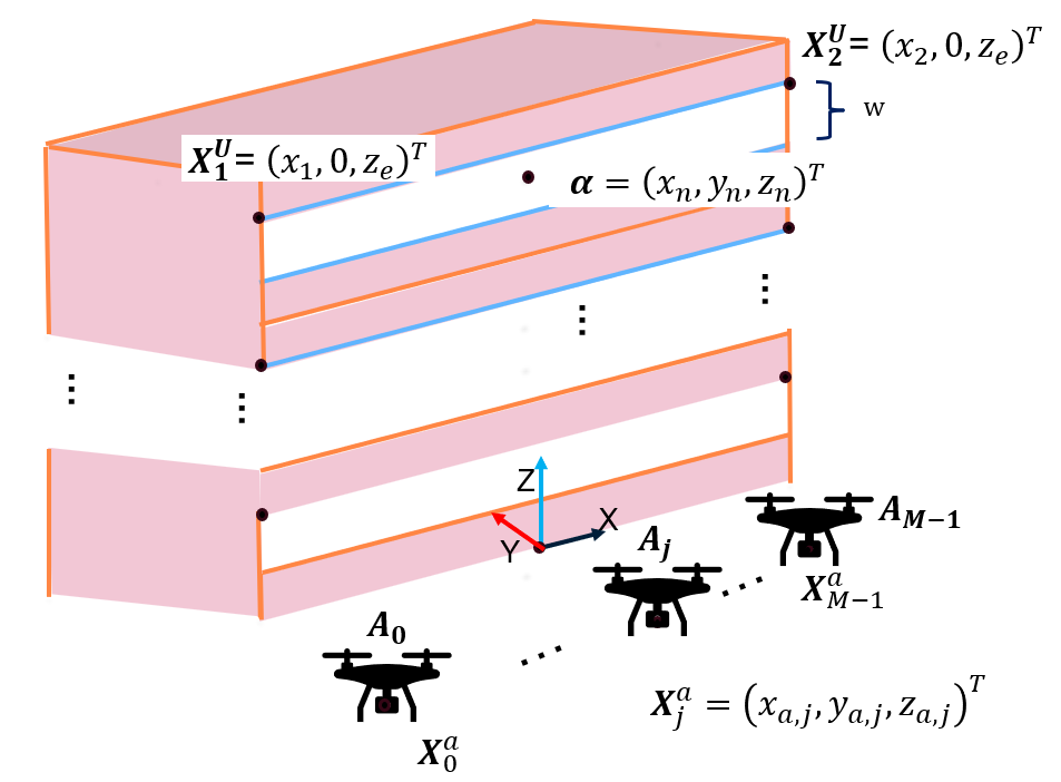
Figure 3: 3D Positioning model for FIM analysis

Each anchor indexed by ‘$j$’ is positioned at known coordinates $\bm{X}^{a}_{j}=[x_{a,j},y_{a,j},z_{a,j}]^{T}$ relative to the origin, while the node is located on an arbitrary floor of the building at $\bm{\alpha}=[x_{n},y_{n},z_{n}]^{T}$. Assuming the anchors are transmitting x-polarized signals, each TOF-based ranging measurement corresponds to the path length of the respective dominating diffraction MPC between each anchor $j$ and the node. With a slight change in notation, we denote the path length of the respective dominating diffraction MPC as $p_{j}(\bm{\alpha})$ obtained using eq. (12), with the subscript ‘j’ representing the $j^{th}$ anchor. Consequently, we obtain $M$ noisy ranging measurements from which we need to estimate the 3D position of the node. Assuming the 3D position of the node $\bm{\alpha}$ as the vector of the three parameters to be estimated, its corresponding Fisher Information Matrix (FIM) $\bm{J}_{\bm{\alpha}}\in\mathbb{R}^{3\times 3}$ [37], [38] and can be expressed as

$$\bm{J}_{\bm{\alpha}}=c^{2}\bm{J}\bm{J}_{\tau_{0}}\bm{J}^{T}.$$ (19)

Since we assume the noise in our range measurements is independent across the $M$ anchors, $\bm{J}_{\tau_{0}}=diag(\lambda_{0},\cdots,\lambda_{M-1})$ is a diagonal matrix where $\lambda_{j}=\frac{1}{8\pi^{2}\beta^{2}SNR_{j}}$ represents the inverse of the CRLB of the path delay estimate of the first arriving path between the $j^{th}$ anchor and the node. The Jacobian $\bm{J}\in\mathbb{R}^{3\times M}$ is the transform from the ranging measurement space $\in\mathbb{R}^{M}$ to the unknown parameter to be estimated space $\in\mathbb{R}^{3}$ and is given by

$$\bm{J}=\begin{bmatrix}\frac{\partial{p_{0}(\bm{\alpha})}}{\partial x_{n}}&\cdots&\frac{\partial{p_{M-1}(\bm{\alpha})}}{\partial x_{n}}\\ \frac{\partial{p_{0}(\bm{\alpha})}}{\partial y_{n}}&\cdots&\frac{\partial{p_{M-1}(\bm{\alpha})}}{\partial y_{n}}\\ \frac{\partial{p_{0}(\bm{\alpha})}}{\partial z_{n}}&\cdots&\frac{\partial{p_{M-1}(\bm{\alpha})}}{\partial z_{n}}\end{bmatrix}.$$ (20)

The node’s unknown 3D coordinates $\bm{\alpha}$ are estimatable if and only if the FIM $\bm{J}_{\bm{\alpha}}$ is invertible [39], therefore in the further analysis we study the conditions for its invertibility.

Theorem 2.

The FIM $\bm{J}_{\bm{\alpha}}\in\mathbb{R}^{3\times 3}$ defined in eq. (19) is invertible if and only if $rank(\bm{J})=3$. Here, the Jacobian Matrix $\bm{J}\in\mathbb{R}^{3\times M}$ is defined in eq. (20) from the TOF ranging measurement space $\mathbb{R}^{M}$ to the 3D coordinate space $\bm{\alpha}\in\mathbb{R}^{3}$.

Proof:

From eq. (19), observe that $\bm{J}_{\tau_{0}}\in\mathbb{R}^{M\times M}$ is a diagonal matrix with non zero diagonal entries since it represents the FIM of the independent ranging measurements from ‘$M$’ anchors. Hence, we can write

$$\bm{J}_{\bm{\alpha}}=c^{2}\bm{J}\bm{J}_{\tau_{0}}\bm{J}^{T}=c^{2}\bm{J}\sqrt{\bm{J}_{\tau_{0}}}\left(\sqrt{\bm{J}_{\tau_{0}}}\bm{J}\right)^{T}.$$

$\sqrt{\bm{A}}$ is the elementwise square root operation of a matrix $\bm{A}$. We also know that multiplying a matrix with a non-zero diagonal matrix does not change its rank. Further, by using $rank(\bm{A}\bm{A}^{T})=rank(\bm{A})$ [40], we obtain $rank(\bm{J}_{\bm{\alpha}})=rank(\bm{J})$. Now, $\bm{J}_{\bm{\alpha}}$ is invertible if and only if $rank(\bm{J}_{\bm{\alpha}})=3$. Hence, we obtain the desired result. ∎

Corollary 3.

To obtain the 3D position estimate for the node at $\bm{\alpha}=[x_{n},y_{n},z_{n}]^{T}$ for the scenario shown in Fig. 3 the following conditions must be met:

• It is necessary but not sufficient to have at least three anchors. This is because, for $rank(\bm{J})=3$, it is necessary but not sufficient to have $M\geq 3$.

• The position of the anchors $\bm{X}^{a}_{j}=[x_{a,j},y_{a,j},z_{a,j}]^{T}\;\forall j\in[0,M-1]$ is known in local building coordinates.

• The x-coordinates of the endpoints of the upper edges of the diffracting edges i.e., $x_{1}$ in $\bm{X}_{1}^{U},x_{2}$ in $\bm{X}_{2}^{U}$ and the window dimension $w$ need to be known a priori.

• The $Z$-coordinate $z_{e}^{u}$ of the diffracting edges on the node building floor is not required to be known.

To illustrate that having $M=3$ anchors is not a sufficient condition for 3D positioning, consider a scenario where we have three anchors such that their x-coordinate $x_{a,j}=0\;\;\forall\;\;j\in[0,2]$. Observe that as the node position is varied inside the building such that it approaches the plane $X=0$, i.e., $x_{n}\to 0$, for each anchor, we have the x-coordinate of the corresponding diffraction point $q_{x}\to 0$. Notice in the first row of the Jacobian $J$, defined in eq. (-E), the term $\frac{\partial p_{j}{(\bm{\alpha}})}{\partial x_{n}}\to 0\;\;\forall j\in[0,2]$. Therefore, for $x_{n}=0$, $rank(J)\neq 3$, and by using Theorem 2, we cannot estimate the 3D position of the node for this scenario.

The diffracting edges are located parallel to the X-axis at $Y=0$. Observe the x-coordinates of the end points of the diffracting edges correspond to the width of the building which is required to be known a priori whereas the height of the diffracting edges is not required to be known. This is because the node and the edge from which diffraction takes place are located on the same building floor. Therefore, by estimating the node location leads to an estimate of the height of the edge since the diffracting edge is located at a distance $\frac{w}{2}$ above the node. Note corollary 3 leads to the following observation - we need position knowledge of the anchors in local building coordinates. These local coordinates are defined with respect to the origin located on the diffracting edges as shown in Fig. 3.

One of the ways to realize a real system, from Corollary 3, is to equip the UAV anchors with GNSS systems, which will provide position knowledge in a global coordinate frame. The translation of these global anchor coordinates to the local building coordinates can be obtained by using map information about the building where the edges of the building can be positioned in the global frame. Alternatively, in areas where GNSS systems may not work accurately, we could use different kinds of sensors to place the anchors in the local building frame. For example, the distance of the anchor to the building $y_{a,j}$ can be obtained using lidar or a laser range finder to the building wall, the elevation of the UAV anchor from the ground $z_{a,j}$ can be obtained using barometers and $x_{a,j}$ can be obtained with inter-anchor TOF ranging measurements.

V Numerical Results

In this section, we lower bound the achievable performance by numerically simulating the analytical CRLB expression in previous sections for a public safety scenario. We demonstrate both the 3D and Z-axis positioning performance in NLOS scenarios can be improved with our positioning technique. A Linear Least Squares (LLS) technique [38] estimation technique is used as a baseline comparison to our proposed positioning technique. Previously, LLS has been shown to achieve its CRLB under the assumption that the Gaussian noise in ranging measurements is much smaller than the path lengths between the anchors and the node [41]. The baseline comparison is a model mismatch scenario, where for the NLOS scenario, the ranging measurements are noisy measurements of the the diffraction paths, whereas, LLS assumes Euclidean path lengths.

For the simulation, each building floor contains a window and we consider $M=3$ anchors located on one side of the building at fixed known coordinates. The numerical values for the other simulation parameters are shown in Table V. As a performance metric, we look at the Position Error Bound (PEB) [39], which is a lower bound on the position estimate of any unbiased estimator. The 3D PEB is defined to be $\sqrt{\mathbb{T}\{(\bm{J}^{-1}_{\bm{\alpha}})\}}$ where the operator $\mathbb{T}\{.\}$ is the trace of a square matrix and $\bm{J}^{-1}_{\bm{\alpha}}$ is the inverse of the FIM defined in eq. (19). Similarly, the bound on the Z-axis is defined to be $\sqrt{{(\bm{J}^{-1}_{\bm{\alpha}})}^{[3,3]}}$, where the notation $\bm{A}^{[i,j]}$ represents the element in the $i^{th}$ row and $j^{th}$ column of matrix $\bm{A}$.

Finally, we uniformly sample $100,000$ points representing candidate node locations $\bm{\alpha}$ within a cuboidal shaped building. For the simulation we consider a cuboidal volume such that $[-10,0,5]^{T}\leq\bm{\alpha}\leq[10,20,40]^{T}$, where the $\leq$ operator between two vectors represents an element-wise operation. Thus, we obtain the 3D-PEB and Z-PEB values for possible node locations within the building. The final results are plotted as a cumulative density histogram in Fig. 4(a) and Fig. 4(b) respectively. The baseline positioning method despite the high SNR is unable to deal with NLOS bias in the ranging measurements and thus offers poor performance. Positioning based on ranging measurements using the diffraction path model hugely improves both the 3D and Z-axis positioning estimates by directly estimating the NLOS path length and is only limited in performance due to system parameters like signal bandwidth and noise figure.

TABLE V: Simulation Parameters.

Description	Symbol & Value
Anchor $0$ pos.	$\bm{X}_{0}^{a}=[-10m,-20m,-10m]^{T}$
Anchor $1$ pos.	$\bm{X}_{1}^{a}=[0m,-7m,-20m]^{T}$
Anchor $2$ pos.	$\bm{X}_{2}^{a}=[10m,-20m,-10m]^{T}$
Building endpoint $1$	$x_{1}=-10m$
Building endpoint $2$	$x_{2}=10m$
window height	$w=2m$
Signal Bandwidth	$\beta=100$ MHz
Signal-to-Noise Ratio	SNR $\in[3dB,6dB,9dB,12dB,15dB]$

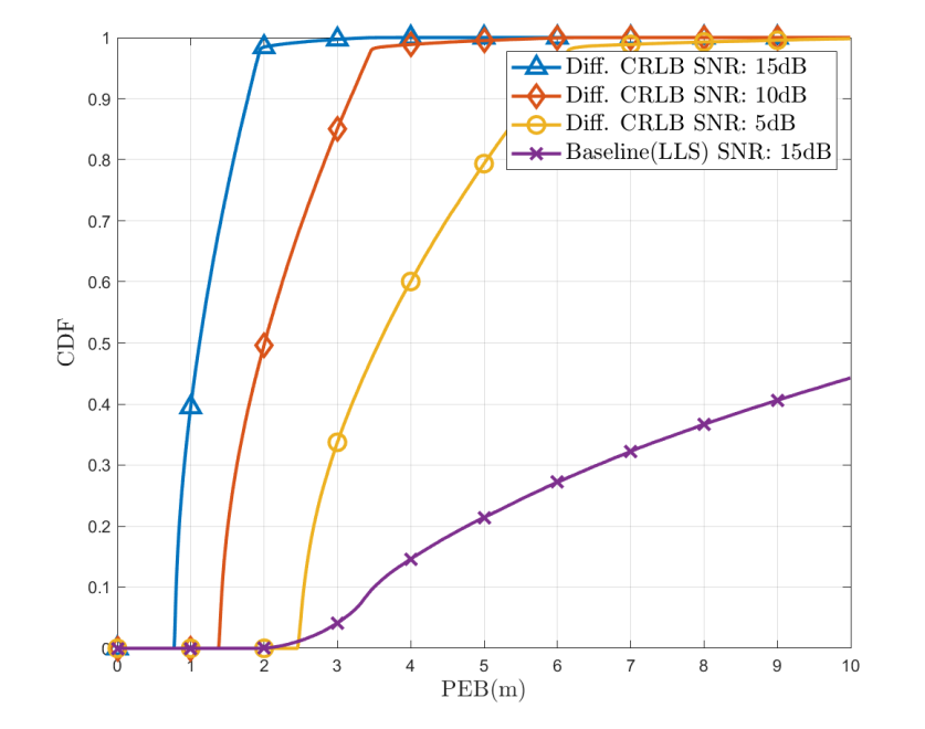
(a) 3D Positioning Performance

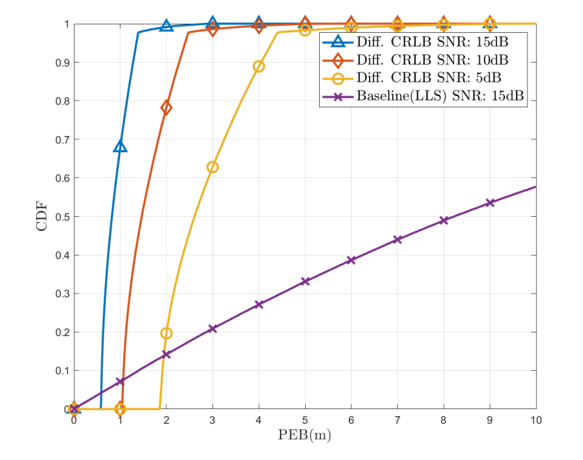
(b) $Z$-axis Positioning Performance

Figure 4: Positioning Performance comparison of the proposed diffraction inspired positioning technique vs the baseline. The NLOS diffraction path model mitigates the NLOS bias problem by estimating the NLOS path length directly and is only limited in performance by the system parameters like noise figure and Bandwidth.

VI Conclusion

In this paper, we investigate positioning in NLOS scenarios and investigate diffraction as a signal propagation mechanism. Using the Geometrical Theory of Diffraction, we develop a new path model for NLOS scenarios where a propagation path is generated due to interaction with an edge. We create a positioning technique based on this approach that can inherently estimate the position of the diffraction point on the diffracting edge. Using Fisher information analysis, we present the necessary and sufficient conditions to estimate the 3D position. Further, we calculate the CRLB on the 3D positioning performance. This positioning approach is then applied to a practical scenario relevant to public safety where there is a need to improve both 3D and Z-axis position estimates. For this, we use a realistic building model that provides insights into signal propagation in the O2I scenario. We present system insights where we control the power in the MPCs generated due to interactions in the window using electric field polarization at the transmitter. Next, we illustrate various ways to achieve the necessary and sufficient conditions to enable 3D position estimates for this system. Finally, we present some numerical results on the lower bound of the positioning performance.

-A Derivation of the path length

Consider Fig. 1(a); our goal is to derive the geometrical path length $AQ_{e}B$. We start by calculating the coordinates of the diffraction point $Q_{e}$. For this, we substitute the incident ray unit vector $\hat{s^{\prime}}$, edge unit vector $\hat{e}$ and diffracted ray unit vector $\hat{s}$ in terms of the various coordinates shown in Fig. 1(a) in the diffraction law eq. (2). Next, we substitute the parametric coordinates of diffraction point $Q_{e}$ in terms of the parameter $\lambda$ and the endpoints of the edge $X_{1}$ and $X_{2}$. After some algebraic manipulations, we obtain a quadratic equation for the parameter $\lambda$. All these steps are shown in eq. (21).

$$\begin{split}&\left|\frac{(q_{x}-x_{a})\hat{x}-y_{a}\hat{y}+(z_{e}-z_{a})\hat{z}}{\sqrt{(q_{x}-x_{a})^{2}+y_{a}^{2}+(z_{e}-z_{a})^{2}}}\cdot\hat{x}\right|=\left|\frac{(x_{n}-q_{x})\hat{x}+y_{n}\hat{y}+(z_{n}-z_{e})\hat{z}}{\sqrt{(x_{n}-q_{x})^{2}+y_{n}^{2}+(z_{n}-z_{e})^{2}}}\cdot\hat{x}\right|\\ &\Rightarrow\left|\frac{(q_{x}-x_{a})}{\sqrt{(q_{x}-x_{a})^{2}+y_{a}^{2}+(z_{e}-z_{a})^{2}}}\right|=\left|\frac{(x_{n}-q_{x})}{\sqrt{(x_{n}-q_{x})^{2}+y_{n}^{2}+(z_{n}-z_{e})^{2}}}\right|\\ &\Rightarrow(q_{x}-x_{a})^{2}((x_{n}-q_{x})^{2}+y_{n}^{2}+(z_{n}-z_{e})^{2})=(x_{n}-q_{x})^{2}((q_{x}-x_{a})^{2}+y_{a}^{2}+(z_{e}-z_{a})^{2})\\ &\Rightarrow(\lambda(x_{1}-x_{2})+x_{2}-x_{a})^{2}((x_{n}-(\lambda(x_{1}-x_{2})+x_{2})))^{2}+y_{n}^{2}+(z_{n}-z_{e})^{2})\\ &\;\;\;\;\;\;\;=(x_{n}-(\lambda(x_{1}-x_{2})+x_{2}))^{2}(((\lambda(x_{1}-x_{2})+x_{2})-x_{a})^{2}+y_{a}^{2}+(z_{e}-z_{a})^{2})\\ &\Rightarrow a\lambda^{2}+b\lambda+c=0.\end{split}$$ (21)

-B Derivation Of Soft Diffraction Coefficients For The Simplified Building Model

Starting from eq. (9), we use the cosine of a sum of angles identities and then the half angle identities $\sin\frac{\psi}{2}=\sqrt{\frac{1-\cos\psi}{2}}$, $\cos\frac{\psi}{2}=\sqrt{\frac{1+\cos\psi}{2}}$. Using the values of $\psi$ and $\psi^{\prime}$ from Table III for the two edges, we arrive at the final expressions in Table IV.

$$\begin{split}D_{s}&=A\left(\frac{1}{\cos\frac{\psi-\psi^{\prime}}{2}}-\frac{1}{\cos\frac{\psi+\psi^{\prime}}{2}}\right)\\ &=A\left(\frac{-2\sin\frac{\psi}{2}\sin\frac{\psi^{\prime}}{2}}{(\cos\frac{\psi}{2}\cos\frac{\psi^{\prime}}{2})^{2}-(\sin\frac{\psi}{2}\sin\frac{\psi^{\prime}}{2})^{2}}\right)\\ &=A\left(\frac{-2\sqrt{1-\cos\psi^{\prime}}}{\cos\psi^{\prime}}\right).\end{split}$$ (22)

-C Power Ratio Of The Diffraction MPCs

Observe that in eq. (13), if the incident electric field is x-polarized i.e., $E_{0,y}=E_{0,z}=0$ the electric field expression simplifies to

$$\begin{split}\bm{E}^{d}&=\begin{aligned} \left(E_{0x}\hat{\bm{\beta}}_{0x}^{\prime}D_{s}\right)\left(\hat{\beta}_{0x}\hat{x}+\hat{\beta}_{0y}\hat{y}+\hat{\beta}_{0z}\hat{z}\right)\\ \end{aligned}\frac{\mathrm{e}^{-jk(|s^{{}^{\prime}}|+|s|)}}{|s^{{}^{\prime}}|\sqrt{|s|}}.\end{split}$$ (23)

Observe, by controlling the polarization, we have eliminated the hard diffraction coefficient from our electric field expression. Now, we calculate the ratio of the squared magnitude of this simplified electric field expression and then substitute the approximated soft diffraction coefficients derived in Lemma 2 and presented in Table IV. Note that $|s^{\prime}|$ and $|s|$ are the OPL and IPL defined in Corollary 1 respectively and are of similar length according to Assumption 2. The power ratio result follows from this.

-D RayTracing Simulation

We set up a model of a brick building in a realistic wireless RayTracing software [42] as shown in Fig.  5. The UAV transmitter was placed 10m away from the exterior of the building. Further, we consider candidate receiver locations spread across five building floors, where each floor is located above the UAV transmitter height. Therefore, this would represent NLOS conditions for most of the locations on these floors. In line with the observation in Bas et al. [32], for each NLOS receiver location, we assume the direct path is sufficiently attenuated, and all the MPCs are generated due to interactions with the windows. We also assume that the windows are made of plain glass, so the attenuation offered to the impinging wireless signal is negligible [43]. The dimensions of each building floor are $20m\times 20m$, and we consider $N_{rx}=8000$ uniformly sampled receiver locations across the five floors of the building.

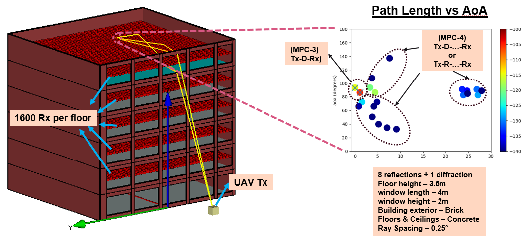
Figure 5: RayTracing setup using Remcom’s Wireless Insight [42] with the different MPC groups labeled on an AoA vs path length plot for an RX location on the $5^{th}$ floor of the building near the back.

For an arbitrary Rx location, the path followed by a particular MPC can be represented as a string such as ‘Tx-X-X-$\cdots$-X-Rx’. Since the MPC begins at the transmitter and terminates at the receiver, all possible strings start with a ‘Tx’ and terminate with an ‘Rx’. The character ‘X’ in the string denotes either ‘R’ or ‘D’ representing ‘Reflection’ or ‘Diffraction’. By reflection, we mean specular reflection from flat surfaces following Snell’s laws, whereas diffraction is from edges and follows the diffraction law in eq. (2). The number of characters ‘X’ between the ‘Tx’ and ‘Rx’ represents the number of interactions, and the left to right order of the characters denotes the sequence of interactions. For our model in Fig. 5, reflections happen at flat surfaces like ceilings, walls, and floors, whereas diffraction happens at edges like the window edges.

TABLE VI: MPC Through The Windows.

Group	MPC-1	MPC-2	MPC-3	MPC-4
String	Tx-Rx	Tx-R-Rx	Tx-D-Rx	Tx-R-R-$\cdots$-Rx or Tx-D-R-$\cdots$-Rx
$P_{e}$	$9.77\%$	$14.41\%$	$93.09\%$	$100\%$
$P_{fap}$	$9.77\%$	$0.23\%$	$82.30\%$	$7.67\%$

For each Rx location, we have many MPCs formed, and we group the MPCs in four unique groups: (a) MPC-1, (b) MPC-2, (c) MPC-3, and (d) MPC-4 based on the propagation mechanism and number of interactions associated with the group. Table VI shows the four possible MPC groups, with the string in the second row representing the corresponding propagation mechanism. Now we evaluate two metrics across all receiver locations (a) Probability of existence: $P_{e}$ and (b) Probability of first arrival path: $P_{fap}$ for the four MPC groups. Mathematically we can express $P_{e}$ and $P_{fap}$ as

$$\begin{split}P_{e}=\frac{N_{e}\times 100}{N_{rx}},\;\;\;P_{fap}=\frac{N_{fap}\times 100}{N_{rx}}.\end{split}$$ (24)

Here, $N_{e}$ is the number of Rx locations where a particular MPC group exists, and $N_{fap}$ is the number of Rx locations where the first arriving path belongs to a particular MPC Group. In Fig. 5, we also plot an AoA vs normalized path length plot for an Rx location at the back of the building. The normalized path length is calculated by subtracting the path length of the first arriving path. Hence, the length of the first arriving path is $0m$. The AoA is defined as the elevation angle from the Z-axis. We present three key observations about the different MPC groups based on Table VI and the AoA vs Path length plot.

Observation 1.

For MPC-1 and MPC-2, we have a low probability of existence $P_{e}$.

Remark.

From the associated string in Table VI, MPC-1 contains MPCs that follow the direct Euclidean path (LOS path) between the transmitter and receiver, whereas MPC-2 contains MPCs that undergo a single bounce satisfying Snell’s laws before reaching the receiver. The low probability of existence can be attributed to the fact that both these MPC groups only exist for Rx locations close to the windows.

Observation 2.

For MPC-3, we have a high probability of existence - $P_{e}=93.09\%$ and also a high probability that the first arriving path belongs to MPC-3 - $P_{fap}=82.3\%$. Lastly, the elevation AoA for MPC-3 is approximately $90$°.

Remark.

The raytracing simulation results show two diffraction paths being generated due to the upper and lower edges of the window on the Rx floor as predicted from the simplified building model presented in Section III-A. Further, from the path length vs AoA plot in Fig. 5, observe that the elevation AoA for the diffraction MPCs is 90°. This is evidence for proposition 1 where the diffraction MPCs arrive at the receiver parallel to the ground. For Rx locations occluded by the vertical pillar between windows, we would have no edge diffraction; instead, ‘Tx-D-Rx’ paths would be as a result of corner diffraction, which is not modeled in Wireless Insight, therefore $P_{e}\neq 100\%$. The first arriving path also happens to be contained in MPC-3 with the highest probability since $P_{fap}=82.3\%$. This is expected since the diffraction field follows the shortest path and was the basis for deriving the path length for the diffraction MPCs using Fermat’s principle of least time in Lemma 1.

Observation 3.

For MPC-4, the MPCs contained in this have varying path lengths and AoA.

Remark.

Since these MPCs undergo several interactions with the window and reflections from the insides of the building, we see varying path lengths and AoAs. Note that even if we were to account for corner diffractions, some MPCs with multiple interactions might be the shortest paths for a select few Rx locations. However, numerical results from the raytracing simulation show these Rx locations are in the minority.

-E Jacobian of the path length $p_{j}(\bm{\alpha})$

The entries in the Jacobian matrix $J$ in eq. (20) can be derived by using the chain rule on the path length $p_{j}(\bm{\alpha})$ between the $j^{th}$ anchor to the node at $\bm{\alpha}$ given by eq. (12). For each anchor, we obtain the x-coordinate $q_{x}$ of the diffraction point $Q_{e}$ on the diffracting edge by the expressions in Lemma 1 with the coefficients of the quadratic $a,b,c$ defined in eq. (4) for each anchor with $z_{e}=z_{n}+0.5w$. For notational simplicity, drop the subscript $j$, and argument $\bm{\alpha}$ in the expression for the entries in the Jacobian. Hence, the path length is denoted as $p$ and is defined for the anchor at $[x_{a},y_{a},z_{a}]^{T}$, the node at $[x_{n},y_{n},z_{n}]^{T}$ and the window size is $w$. The final expression is below.

$$\begin{split}\frac{\partial p}{\partial x_{n}}&=\frac{(q_{x}-x_{a})\frac{\partial q_{x}}{\partial x_{n}}}{\sqrt{(q_{x}-x_{a})^{2}+(y_{a})^{2}+(z_{a}-z_{n}-0.5w)^{2}}}\\ &\;\;\;\;\;\;\;\;\;\;\;\;\;\;\;\;\;\;\;\;\;\;\;+\frac{(x_{n}-q_{x})(1-\frac{\partial q_{x}}{\partial x_{n}})}{\sqrt{(x_{n}-q_{x})^{2}+(y_{n})^{2}+(0.5w)^{2}}},\\ \frac{\partial p}{\partial y_{n}}&=\frac{(q_{x}-x_{a})\frac{\partial q_{x}}{\partial y_{n}}}{\sqrt{(q_{x}-x_{a})^{2}+(y_{a})^{2}+(z_{a}-z_{n}-0.5w)^{2}}}\\ &\;\;\;\;\;\;\;\;\;\;\;\;\;\;\;\;\;\;\;\;+\frac{(q_{x}-x_{n})\frac{\partial q_{x}}{\partial y_{n}}+y_{n}}{\sqrt{(x_{n}-q_{x})^{2}+(y_{n})^{2}+(0.5w)^{2}}},\\ \frac{\partial p}{\partial z_{n}}&=\frac{(q_{x}-x_{a})\frac{\partial q_{x}}{\partial z_{n}}}{\sqrt{(q_{x}-x_{a})^{2}+(y_{a})^{2}+(z_{a}-z_{n}-0.5w)^{2}}}\\ &\;\;\;\;\;\;\;\;\;\;\;\;\;\;\;\;\;\;\;\;+\frac{(q_{x}-x_{n})\frac{\partial q_{x}}{\partial z_{n}}}{\sqrt{(x_{n}-q_{x})^{2}+(y_{n})^{2}+(0.5w)^{2}}},\\ \frac{\partial q_{x}}{\partial x_{n}}&=\frac{(x_{1}-x_{2})}{2a}\left[\frac{\partial a}{\partial x_{n}}\left(\frac{(b\mp\sqrt{b^{2}-4ac}}{a}\right)\right.\\ &\left.\;\;\;\;\;\;\;\;\;\;\;\;+\left(-\frac{\partial b}{\partial x_{n}}\pm\frac{b\frac{\partial b}{\partial x_{n}}-2c\frac{\partial a}{\partial x_{n}}-2a\frac{\partial c}{\partial x_{n}}}{\sqrt{b^{2}-4ac}}\right)\right],\\ \end{split}$$

$$\begin{split}\frac{\partial q_{x}}{\partial y_{n}}&=\frac{(x_{1}-x_{2})}{2a}\left[\frac{\partial a}{\partial y_{n}}\left(\frac{(b\mp\sqrt{b^{2}-4ac}}{a}\right)\right.\\ &\left.\;\;\;\;\;\;\;\;\;\;\;\;+\left(-\frac{\partial b}{\partial y_{n}}\pm\frac{b\frac{\partial b}{\partial y_{n}}-2c\frac{\partial a}{\partial y_{n}}-2a\frac{\partial c}{\partial y_{n}}}{\sqrt{b^{2}-4ac}}\right)\right],\\ \frac{\partial q_{x}}{\partial z_{n}}&=\frac{(x_{1}-x_{2})}{2a}\left[\frac{\partial a}{\partial z_{n}}\left(\frac{(b\mp\sqrt{b^{2}-4ac}}{a}\right)\right.\\ &\left.\;\;\;\;\;\;\;\;\;\;\;\;+\left(-\frac{\partial b}{\partial z_{n}}\pm\frac{b\frac{\partial b}{\partial z_{n}}-2c\frac{\partial a}{\partial z_{n}}-2a\frac{\partial c}{\partial z_{n}}}{\sqrt{b^{2}-4ac}}\right)\right],\\ \frac{\partial a}{\partial x_{n}}&=0,\;\frac{\partial a}{\partial y_{n}}=2y_{n}(x_{1}-x_{2})^{2},\frac{\partial a}{\partial z_{n}}=2(x_{1}-x_{2})^{2}(z_{n}+\frac{w}{2}),\\ \frac{\partial b}{\partial x_{n}}&=2(x_{1}-x_{2})\left((z_{1}-z_{a})^{2}+y_{a}^{2}\right),\\ \frac{\partial b}{\partial y_{n}}&=4y_{n}(x_{1}-x_{2})(x_{2}-x_{a}),\\ \frac{\partial b}{\partial z_{n}}&=-4(x_{1}-x_{2})(x_{2}-x_{n})(z_{n}+\frac{w}{2}-z_{a}),\\ \frac{\partial c}{\partial x_{n}}&=2(x_{2}-x_{n})\left((z_{1}-z_{a})^{2}+y_{a}^{2}\right),\\ \frac{\partial c}{\partial y_{n}}&=2y_{n}(x_{2}-x_{a})^{2},\frac{\partial c}{\partial z_{n}}=-2(x_{2}-x_{n})^{2}(z_{n}+\frac{w}{2}-z_{a}).\end{split}$$ (25)

References

- [1] G. Duggal, R. M. Buehrer, H. S. Dhillon, and J. H. Reed, “3D Positioning using a new diffraction path model,” Proc., IEEE Intl. Conf. on Commun. (ICC), 2024.
- [2] E. D. Kaplan and C. Hegarty, Understanding GPS/GNSS: principles and applications. Artech house, 2017.
- [3] S. Dwivedi, R. Shreevastav, F. Munier, J. Nygren, I. Siomina, Y. Lyazidi, D. Shrestha, G. Lindmark, P. Ernström, E. Stare et al., “Positioning in 5G networks,” IEEE Commun. Magazine, Nov 2021.
- [4] Y. Shen and M. Z. Win, “Fundamental limits of wideband localization—Part I: A general framework,” IEEE Trans. on Info. Theory, 2010.
- [5] C. E. O’Lone, H. S. Dhillon, and R. M. Buehrer, “Characterizing the first-arriving multipath component in 5G millimeter wave networks: TOA, AOA, and non-line-of-sight bias,” IEEE Trans. on Wireless Commun., 2022.
- [6] Y. Qi, H. Kobayashi, and H. Suda, “Analysis of wireless geolocation in a non-line-of-sight environment,” IEEE Trans. on Wireless Commun., 2006.
- [7] T. Jia and R. M. Buehrer, “A set-theoretic approach to collaborative position location for wireless networks,” IEEE Trans. Mobile Computing, Dec 2010.
- [8] ——, “Collaborative position location with NLOS mitigation,” Proc., IEEE PIMRC, Dec 2010.
- [9] S. Venkatesh and R. M. Buehrer, “NLOS mitigation using linear programming in ultrawideband location-aware networks,” IEEE Trans. on Veh. Technology, 2007.
- [10] R. M. Vaghefi, J. Schloemann, and R. M. Buehrer, “NLOS mitigation in TOA-based localization using semidefinite programming,” in 2013 10th Workshop on Positioning, Navigation and Communication (WPNC), 2013.
- [11] K. Witrisal, P. Meissner, E. Leitinger, Y. Shen, C. Gustafson, F. Tufvesson, K. Haneda, D. Dardari, A. F. Molisch, A. Conti, and M. Z. Win, “High-accuracy localization for assisted living: 5G systems will turn multipath channels from foe to friend,” IEEE Signal Processing Magazine, Mar 2016.
- [12] E. Leitinger, P. Meissner, C. Rüdisser, G. Dumphart, and K. Witrisal, “Evaluation of position-related information in multipath components for indoor positioning,” IEEE Journal on Sel. Areas in Commun., Nov 2015.
- [13] R. Mendrzik, H. Wymeersch, G. Bauch, and Z. Abu-Shaban, “Harnessing NLOS components for position and orientation estimation in 5G millimeter wave MIMO,” IEEE Trans. on Wireless Commun., Dec 2019.
- [14] H. Naseri and V. Koivunen, “Cooperative simultaneous localization and mapping by exploiting multipath propagation,” IEEE Trans. on Signal Processing, 2017.
- [15] C. Gentner, T. Jost, W. Wang, S. Zhang, A. Dammann, and U.-C. Fiebig, “Multipath assisted positioning with simultaneous localization and mapping,” IEEE Trans. on Wireless Commun., 2016.
- [16] M. A. Nazari, G. Seco-Granados, P. Johannisson, and H. Wymeersch, “MmWave 6D radio localization With a snapshot observation from a single BS,” IEEE Trans. on Veh. Technology, 2023.
- [17] FirstNet Authority. (2023, Sep) First responder network authority roadmap. [Online]. Available: https://www.firstnet.gov/sites/default/files/Roadmap_2023.pdf
- [18] H. K. Dureppagari, D.-R. Emenonye, H. S. Dhillon, and R. M. Buehrer, “UAV-aided indoor localization of emergency response personnel,” in 2023 IEEE/ION PLANS, 2023.
- [19] G. Duggal, R. M. Buehrer, N. Tripathi, and J. H. Reed, “Line-of-sight probability for outdoor-to-indoor UAV-assisted emergency networks,” Proc., IEEE Intl. Conf. on Commun. (ICC), May 2023.
- [20] J. B. Keller, “Geometrical theory of diffraction,” J. Opt. Soc. Am., 1962.
- [21] D. Namara, C. Pistorious, and J. Maherbe, Introduction to the Uniform Geometric Theory of Diffraction. Artech House, 1990.
- [22] C. A. Balanis, Advanced Engineering Electromagnetics. John Wiley & Sons, 2012.
- [23] P. Tenerelli and C. Bostian, “Measurements of 28 GHz diffraction loss by building corners,” in Proc., IEEE PIMRC, 1998.
- [24] Y. L. de Jong, M. H. Koelen, and M. H. Herben, “A building-transmission model for improved propagation prediction in urban microcells,” IEEE Trans. on Veh. Technology, 2004.
- [25] A. Pallaprolu, B. Korany, and Y. Mostofi, “Wiffract: a new foundation for rf imaging via edge tracing,” in Proc. of the 28th Annual Intl. Conf. on Mob. Computing And Networking, 2022.
- [26] ——, “Analysis of Keller cones for rf imaging,” in 2023 IEEE Radar Conference (RadarConf23), 2023.
- [27] M. Born and E. Wolf, Principles of optics: electromagnetic theory of propagation, interference and diffraction of light. Elsevier, 2013.
- [28] Y. Rahmat-Samfi, “Keller’s cone encountered at a hotel,” IEEE Antennas and Propag. Mag., 2007.
- [29] R. G. Kouyoumjian and P. H. Pathak, “A uniform geometrical theory of diffraction for an edge in a perfectly conducting surface,” Proceedings of the IEEE, 1974.
- [30] A. Albanese, V. Sciancalepore, and X. Costa-Pérez, “First responders got wings: UAVs to the rescue of localization pperations in beyond 5G systems,” IEEE Commun. Magazine, 2021.
- [31] M. Kohli, A. Adhikari, G. Avci, S. Brent, A. Dash, J. Moser, S. Hossain, I. Kadota, C. Garland, S. Mukherjee, R. Feick, D. Chizhik, J. Du, R. A. Valenzuela, and G. Zussman, “Outdoor-to-Indoor 28 GHz wireless weasurements in Manhattan: path loss, environmental effects, and 90% coverage,” IEEE/ACM Trans. on Networking, 2024.
- [32] C. U. Bas, R. Wang, S. Sangodoyin, T. Choi, S. Hur, K. Whang, J. Park, C. J. Zhang, and A. F. Molisch, “Outdoor to indoor propagation channel measurements at 28 GHz,” IEEE Trans. on Wireless Commun., 2019.
- [33] F. Sikta, W. Burnside, T.-T. Chu, and L. Peters, “First-order equivalent current and corner diffraction scattering from flat plate structures,” IEEE Trans. on Antennas and Propagation, 1983.
- [34] R. W. Heath, N. Gonzalez-Prelcic, S. Rangan, W. Roh, and A. M. Sayeed, “An overview of signal processing techniques for millimeter wave MIMO systems,” IEEE Journal on Sel. Areas in Signal Processing, Feb 2016.
- [35] C. Falsi, D. Dardari, L. Mucchi, and M. Z. Win, “Time of arrival estimation for UWB localizers in realistic environments,” EURASIP Journal on Adv. in Sig. Process., 2006.
- [36] H. L. Van Trees, Detection, Estimation, and Modulation Theory, part I: Detection, Estimation, and Linear Modulation Theory. John Wiley & Sons, 2004.
- [37] S. M. Kay, Fundamentals of Statistical Signal Processing: Estimation Theory. Prentice-Hall, Inc., 1993.
- [38] R. Zekavat and R. M. Buehrer, Handbook of Position Location: Theory, Practice and Advances. John Wiley & Sons, 2011.
- [39] D.-R. Emenonye, H. S. Dhillon, and R. M. Buehrer, “RIS-aided localization under position and orientation offsets in the near and far field,” IEEE Trans. on Wireless Commun., May 2023.
- [40] G. Strang, Linear Algebra for Everyone. SIAM, 2020.
- [41] S. Gezici, I. Guvenc, and Z. Sahinoglu, “On the performance of linear least-squares estimation in wireless positioning systems,” in Proc., IEEE Intl. Conf. on Commun. (ICC), 2008.
- [42] Remcom Inc . (2024, July) Wireless InSite MIMO: version 3.4.4. [Online]. Available: https://www.remcom.com
- [43] W. Honcharenko, H. Bertoni, and J. Dailing, “Mechanisms governing propagation between different floors in buildings,” IEEE Trans. on Antennas and Propagation, 1993.