Gyroscopic Gravitational Memory from quasi-circular binary systems

Abstract

Gravitational waves cause a precession in a freely falling spinning object and a net change of orientation after the passage of the wave, dubbed as the gyroscopic memory. In this paper, we will consider isolated gravitational sources in the post-Newtonian framework and compute the gyroscopic precession and memory at leading post-Newtonian (PN) orders. We make a comparison between two competing contributions: the spin memory and the nonlinear helicity flux. At the level of the precession rate, the former is a 2PN oscillatory effect, while the latter is a 4PN adiabatic effect. However, the gyroscopic memory involves a time integration, which enhances subleading adiabatic effects by the fifth power of the velocity of light, leading to a 1.5PN memory effect. We explicitly compute the leading effects for a quasi-circular binary system and obtain the angular dependence of the memory on the celestial sphere.

1 Introduction

Spin and rotation effects play a crucial role in the dynamics of gravitating systems in general relativity (GR). The mass currents arising in rotating bodies source a “gravitomagnetic” potential entering the parametrization of the linearized metric, with no Newtonian counterpart. The primary example of a stationary rotating solution is the Kerr black hole, which has many distinct features from a static black hole of the same mass. Examples of such features include the Lens-Thirring frame dragging [1] and the black hole’s ergosphere, whose interaction with the surrounding matter fields lead to interesting physical effects, such as superradiance [2] and the Blandford–Znajek process [3].

In addition to stationary situations, one must be able to describe the dynamical interaction between gravity and spinning matter. This topic has a rich literature, started by the seminal works of Mathisson and Papapetrou [4, 5], who formulated the motion and precession of a test spinning particle in GR. Their results were rephrased by Tulczyjew, and extended by Dixon and others to include the higher multipole structure of test particles [6, 7, 8, 9]. The Mathisson, Papapetrou, Dixon (MPD) equations may be derived in full generality from an effective worldline action [10], which lays the basis for the effective field theory approach to study the dynamics of self-gravitating systems of spinning particles in the post-Newtonian (PN) framework, as an important class of gravitational-wave (GW) sources (see [11, 12] for the derivation of the PN equations of motion for compact binaries from MPD equations, or [13] for the calculation of the corresponding Fokker Lagrangian, following theoretical grounds elucidated in [14]).

In this paper, we will be interested in spinning bodies as probes of GWs. In particular, we will investigate DC effects of GW that accumulate over time and lead to persistent observables lasting after the passage of the wave [15]. The primary example of such observables is the displacement effect, describing a net change in the distance between nearby freely falling test particles [16, 17, 18, 19, 20]. If the test particle is endowed with a spin, as a gyroscope, an additional observable is the precession of the spin caused by the GWs. Different experiments to measure the effect can be thought of. One consists in comparing the spin of nearby geodesics, as suggested in [15], another one in measuring the precession of the spin of a single gyroscope in an optical frame tied to distant stars. The latter proposal was examined in [21, 22], where it was found that, restricting to the regime in which the spin vector is approximately parallel transported along a geodesic motion, GWs cause a precession in the local transverse plane of the propagation and is proportional to the inverse square of the distance to the source. As a result, the passage of the wave induces in that case a net rotation in the orientation of the gyroscope, dubbed as the “gyroscopic memory”. The dynamics is however more involved when nonlinear spin interactions cannot be neglected so that the full MPD equations must be taken into account. In section 2, we will clarify the limit in which the parallel-transport assumption is valid.

The goal of this paper is to investigate the PN expansion of the gyroscopic memory when the GWs are sourced by binary systems of compact objects. We will actually focus on quasi-circular binaries, consisting of two non-spinning compact bodies on a nearly circular orbit whose radius adiabatically shrinks in time. We will address the following questions: (1) How does the test gyroscope’s precession rate depend on its angular position on the celestial sphere? (2) What is the magnitude of the precession in terms of the parameters of the binary system? (3) What are the DC components of the precession and the accumulation effect resulting in the gyroscopic memory?

The paper is organized as follows. In section 2, we introduce the MPD equations to show how, in a certain limit, the spin evolution reduces to the parallel transport used in deriving the gyroscopic memory effect in [21, 22]. This construction and its implications are reviewed in 2.3. In section 3, we reformulate the precession rate and gyroscopic memory using “spin-weighted” functions on the celestial sphere. The latter approach is advantageous not only formally, due to the simplicity of the resulting expressions, but also for practical computations. Resorting to those tools, it is straightforward to perform the multipole expansion of the precession and to compute memory effects in terms of the radiative moments, which is achieved in section 3. In section 4, we introduce quasi-circular binary systems, discuss their radiation, and compute the precession of a distant freely falling gyroscope as well as the gyroscopic memory in the PN framework. We conclude in section 5, by briefly discussing observational aspects of the gyroscopic memory.

2 Brief review of spin dynamics in general relativity

2.1 Effective approach to spinning objects

The motion and precession of a free point-like body with velocity $v^{\mu}$ (normalized so that $v^{\mu}v_{\mu}=-c^{2}$), momentum $p_{\mu}$, carrying some spin represented by the antisymmetric tensor $S^{\mu\nu}$ is given by the equations [7]

$$\frac{\mathrm{D}p_{\mu}}{\mathrm{D}\tau}=-\frac{1}{2}R_{{\mu\nu}\rho\sigma}v^{\nu}S^{\rho\sigma}-\frac{c^{2}}{6}J^{\nu\lambda\rho\sigma}\nabla_{\mu}R_{\nu\lambda\rho\sigma}+\cdots\,,$$ (1a)

$$\frac{\mathrm{D}S^{\mu\nu}}{\mathrm{D}\tau}=2p^{[\mu}v^{\nu]}+\frac{4c^{2}}{3}R^{[\mu}{}_{\lambda\rho\sigma}J^{\nu]\lambda\rho\sigma}+\cdots\,,$$ (1b)

where $\mathrm{D}/\mathrm{D}\tau\equiv v^{\mu}\nabla_{\mu}$, with the Levi-Civita derivative $\nabla_{\mu}$, and the corresponding Riemann tensor $R^{\mu}_{~{}\nu\rho\sigma}$ are derived from the metric $g_{\mu\nu}$, and the square brackets denote the antisymmetrization over the enclosing indices. The tensor $S^{\mu\nu}$ contains nonphysical degrees of freedoms related to the choice of the body centroid. To fix them, the above equations must be supplemented by a spin supplementary condition [23, 24, 25]. A particularly convenient choice is the covariant Tulczyjew condition $p_{\nu}S^{\mu\nu}=0$ [6, 26, 7], implying that, in the “center-of-mass” frame defined by means of an orthogonal tetrad whose temporal basis vector lies along $p^{\nu}$, the components of the spin vector are purely spatial. The internal structure of the body manifests itself through the Dixon moments, such as the quadrupole tensor $J^{{\mu\nu}\rho\sigma}$, as well as higher-order moments, $J^{\nu\lambda\rho\sigma\tau}$, $J^{\nu\lambda\rho\sigma\tau\upsilon}$, etc., which enter the subleading corrections represented by the dots in (1). It should be emphasized that, when the body is assumed to be in thermodynamical equilibrium at any instant, the Dixon moments are entirely determined by the mass, spin, equation of state and external gravitational field. Notably, if the tidally induced deformation is negligible compared with the spin induced one, the Dixon quadrupole reads [27]

$$J^{{\mu\nu}\rho\sigma} =\frac{3\kappa}{mc^{4}}v^{[\mu}S^{\nu]\lambda}S_{\lambda}{}^{[\rho}v^{\sigma]}\,,$$ (2)

where the dependence on the equation of state arises through the dimensionless constant $\kappa$. Equations (1) and (2) must be thought of as effective and, as such, they do remain valid for self-gravitating systems. It should be noted that only the first terms in the right-hand sides of each equation in (1) are universal, i.e. , independent of the nature of the body, while the others terms containing Dixon moments depend on the system’s equation of state. The full MPD equations for test extended bodies, in the zero radius limit, were first derived by Dixon [9], while Bailey and Israel [10] recovered this result starting from an effective Lagrangian (see [27] for a short modern review). This approach was later incorporated in the effective field theory approach to investigate the dynamics of GW sources [28, 13].

Contracting the momentum with (1b), employing the Leibniz rule, the supplementary condition and (1a) imply that $p_{\nu}\mathrm{D}S^{\mu\nu}/\mathrm{D}\tau=\mathcal{O}(S^{2})\,.$ Using this information in (1b) next reveals that $2p_{\nu}p^{[\mu}v^{\nu]}=\mathcal{O}(S^{2})$. Defining the bare mass as $m\equiv-p^{\mu}v_{\mu}/c^{2}$, it follows that $p^{\mu}p_{\mu}+m^{2}c^{2}=\mathcal{O}(S^{2})$ and $p^{\mu}=mv^{\mu}+\mathcal{O}(S^{2})\,.$ Inserting this back in (1b), we find that

$$\frac{\mathrm{D}S^{\mu\nu}}{\mathrm{D}\tau}=0+\mathcal{O}(S^{2})\,,$$ (3)

i.e. , the spin obeys the parallel transport equation to leading order in the spin. Moreover, the body’s worldline is geodesic up to linear corrections in the spin, namely, $\mathrm{D}v^{\mu}/\mathrm{D}\tau=\mathcal{O}(S^{\mu\nu})$. In the rest of this paper, we will neglect higher order spin corrections and will therefore restrict our attention to the parallel transport along a geodesic. In this regime, it is more convenient to define a spin vector $S^{\mu}\equiv-\varepsilon_{{\mu\nu}\rho\sigma}p^{\nu}S^{\rho\sigma}/(2mc)$, so that, at leading order in the spin, the evolution equations reduce to

$$\frac{\mathrm{D}v^{\mu}}{\mathrm{D}\tau} =0,\qquad\frac{\mathrm{D}S^{\mu}}{\mathrm{D}\tau}=0\,.$$ (4)

2.2 Parallel transport in orthonormal frames

To solve the parallel transport equation for the spin, it is convenient to introduce a local orthogonal frame $e_{a}{}^{\mu}$, normalized as $e_{a}{}^{\mu}e_{b}{}^{\nu}g_{\mu\nu}=\eta_{ab}$. There is no unique choice for this tetrad, the resulting ambiguity being parameterized by local Lorentz transformations of the basis vectors. Exploiting this freedom, the tetrad may be gauge-fixed in a way that helps solving the equation (4) for the spin. After an appropriate choice has been made, the tetrad is entirely fixed, i.e. , the basis vectors $e_{a}{}^{\mu}$ become known functions of the metric as well as possible additional structures, such as the velocity field of the observer, and spacetime coordinates. In this frame, $S^{\mu}=S^{a}e_{a}{}^{\mu}$ evolve as

$$~{}v^{\mu}\partial_{\mu}S^{a}=-v^{\mu}\omega_{\mu}{}^{a}{}_{b}S^{b}\,,\qquad\omega_{\mu}{}^{a}{}_{b}=e^{a}{}_{\alpha}\nabla_{\mu}e_{b}{}^{\alpha}\,,$$ (5)

where $\omega_{\mu}{}^{a}{}_{b}$ is the spin connection associated to the tetrad. The form (5) of the spin precession is however not yet satisfactory. Indeed, on the one hand, neither side of (5) is covariant with respect to local Lorentz transformations $S^{a}\to\Lambda^{a}{}_{b}(x^{\mu})S^{b}$, except for the position-independent subgroup. On the other hand, for a generic choice of the tetrad, the equation predicts the precession of gyroscopes even when embedded in the flat Minkowski background, since the spin connection is not necessarily vanishing in that case. It is yet possible to rewrite it in a way that resolves both issues and highlights its physical content. This may be achieved by adding $v^{\mu}\overline{\omega}_{\mu}{}^{a}{}_{b}S^{b}$ on both sides, where $\overline{\omega}_{\mu}{}^{a}{}_{b}$ is the spin connection with respect to $e_{a}{}^{\mu}$ but defined with the Levi-Civita connection $\overline{\text{D}}_{\mu}$ of a reference background metric (a Minkowski metric $\eta^{{\mu\nu}}$ in this setup). The resulting equation accordingly reads

$$v^{\mu}\overline{\text{D}}_{\mu}S^{a}=-v^{\mu}\left(\omega_{\mu}{}^{a}{}_{b}-\overline{\omega}_{\mu}{}^{a}{}_{b}\right)S^{b}\,,$$ (6)

where we have used that $\overline{\text{D}}_{\mu}S^{a}=\partial_{\mu}S^{a}+\overline{\omega}_{\mu}{}^{a}{}_{b}S^{b}$. Each side of (6) is now covariant under arbitrary local Lorentz transformations $S^{a}\to\Lambda^{a}{}_{b}(x^{\mu})S^{b}$, while the precession vanishes over the background spacetime. We can think of the left-hand side as the spin time evolution with respect to a frame that is parallel transported with the background metric.

For a freely falling gyroscope, it is natural to choose the orthonormal frame to be comoving, i.e. , to take $e_{a}{}^{\mu}=(v^{\mu},e_{{\hat{i}}}{}^{\mu})$, where $e_{{\hat{i}}}{}^{\mu}$ for $\hat{i}=1,2,3$ are the space-like basis vectors, while the temporal basic vector coincides with the geodesic velocity $v^{\mu}$ of the gyroscope. In this frame, the spin is purely spatial and (6) reduces to

$$\dfrac{\text{d}S^{\hat{i}}}{\text{d}\tau}=\Omega^{\hat{i}}{}_{\hat{j}}S^{\hat{j}}\,,\qquad\Omega^{\hat{i}}{}_{\hat{j}}=-v^{\mu}\big{(}\omega_{\mu}{}^{\hat{i}}{}_{{\hat{j}}}-\overline{\omega}_{\mu}{}^{\hat{i}}{}_{{\hat{j}}}\big{)}$$ (7)

where $\text{d}/\text{d}\tau\equiv v^{\mu}\overline{\text{D}}_{\mu}$ and all frame indices are raised or lowered with the Kronecker delta $\delta_{{\hat{i}}{\hat{j}}}$.

This covariant expression requires an additional background structure $\overline{\omega}_{\mu}{}^{\hat{i}}{}_{{\hat{j}}}$, which makes sense in a perturbative analysis, where a background metric is always assumed. In an asymptotic analysis, as we do in the following, a background metric does not directly appear. However, $\overline{\omega}_{\mu}{}^{\hat{i}}{}_{{\hat{j}}}$ is uniquely determined by the fixed boundary structures. In asymptotically flat spacetimes, this boundary structure correspond to the location of “distant stars” on the celestial sphere. Therefore, (7) is interpreted as the time evolution of the spin with respect to a frame tied to distant stars, and the antisymmetric tensor $\Omega^{\hat{i}}{}_{\hat{j}}$ is the precession rate in the ${\hat{i}}{\hat{j}}$ plane.

2.3 Gyroscopes in asymptotically flat spacetimes

2.3.1 Precession equations for asymptotic gyroscopes

The metric far from a localized source of gravitational waves is suitably expressed in Bondi coordinates $(u,r,\theta^{A})$ with $u$ the null retarded time, $r$ the areal distance from the source localized around $r=0$, and $\theta^{A}$ a coordinate system on the sphere. As an asymptotic expansion in $r$, it reads

$$\text{d}s^{2}= -\left(1-\frac{2G\mu}{rc^{2}}+\mathcal{O}\left(\frac{1}{r^{2}}\right)\right)\text{d}u^{2}-2\left(1+\mathcal{O}\left(\frac{1}{r}\right)\right)\text{d}u\,\text{d}r$$

$$+r^{2}\left(\gamma_{AB}+\frac{1}{r}\,C_{AB}+\mathcal{O}\left(\frac{1}{r}\right)\right)\text{d}\theta^{A}\,\text{d}\theta^{B}+\left(\mathrm{D}_{B}C_{A}{}^{B}\text{d}u\,\text{d}\theta^{A}+\mathcal{O}\left(\frac{1}{r}\right)\right)\,,$$ (8)

where the symmetric trace-free tensor $C_{AB}(u,\theta^{A})$ is the Bondi shear and encodes gravitational waves emitted by the source, and $\mu(u,\theta^{A})$ is the Bondi mass aspect. The metric (2.3.1) makes explicit leading order deviations from the Minkowski metric, while “subleading” corrections are not required for the purpose of this paper.

Now consider a gyroscope, located at large but finite distance $r$ from the source. We would like to compute the precession of the spin of the gyroscope with respect to a frame pointing towards distant stars. The details of the construction of the tetrad is given in [21, 22] (see also [29, 30, 31]). Decomposing spatial directions into radial and transverse ${\hat{i}}={\hat{r}},{\hat{A}}$, it was found in [21, 22] that the passage of gravitational waves by the gyroscope induces a dominant precession in the transverse plane given by

$$\Omega_{{\hat{A}}{\hat{B}}}=\frac{\varepsilon_{{\hat{A}}{\hat{B}}}}{r^{2}}\hat{\Omega}+\mathcal{O}\left(\frac{1}{r^{3}}\right)\,,\qquad\hat{\Omega}(u,\theta^{A})=\underbrace{\frac{c}{4}\mathrm{D}_{A}\mathrm{D}_{B}\widetilde{C}^{AB}}_{\hat{\Omega}_{\text{(S)}}}\underbrace{-\frac{1}{8}\dot{C}_{AB}\widetilde{C}^{AB}}_{\hat{\Omega}_{\text{(H)}}}\,,$$ (9)

where $\widetilde{C}_{AB}\equiv\varepsilon_{CA}C^{C}{}_{B}$ is the dual shear and $c$ is the speed of light. The other component is subleading at large distance, $\Omega_{{\hat{r}}{\hat{A}}}=\mathcal{O}(r^{-3})$.

2.3.2 Gyroscopic memory

After the passage of the wave, GWs induce a net rotation in the orientation of the gyroscope in transverse plane, whose angle is simply obtained by the time integral of (9),

$$\Delta\Psi =\frac{\Delta\hat{\Psi}}{r^{2}}+\mathcal{O}\left(\frac{1}{r^{3}}\right)\,,\qquad\Delta\hat{\Psi}=\int_{u_{0}}^{u}\text{d}v\big{(}\hat{\Omega}_{\text{(S)}}(v)+\hat{\Omega}_{\text{(H)}}(v)\big{)}\,.$$ (10)

The precession rate (9) consists of a linear term in the shear and a quadratic term. They are denoted by S and H labels respectively, which is justified in two ways. On the one hand, the time integral in (10) kills all but the zero frequency mode in the Fourier expansion of the linear term, and is thus referred to as soft, while the quadratic term includes gravitons of all frequencies, and is referred to as hard. On the other hand, the first term coincides exactly with the spin memory effect [32, 33, 34, 35], while the second term measures the total helicity, the difference between the number of right-handed and left-handed gravitons at a given point on the celestial sphere [21, 22, 36, 37, 38, 39, 40].

3 Multipole expansion of the precession rate

3.1 Precession in the holomorphic basis

Our main results, Eqs. (9) and (10) involve tensorial expressions constructed out of the symmetric trace-free (STF) Bondi shear and its covariant derivatives with respect to the round metric $\gamma_{AB}$ on the sphere. Remarkably, STF tensors of any rank in two dimensions have only two independent degrees of freedom, which can be combined into a single complex scalar. This correspondence provides an elegant and practical formulation of the problem in terms of spin-weighted functions, which we explain here and further in appendix A. This formalism was developed in the representation theory of the rotation group [41], and independently in the spin-coefficient formalism of Newman and Penrose [42] and is widely used in the context of GW theory.

Given a real orthonormal basis $E_{\hat{1}}{}^{A},E_{\hat{2}}{}^{A}$ on a two-dimensional Riemannian manifold, one can construct a pair of null vectors, consisting of $m^{A}=\tfrac{1}{\sqrt{2}}(E_{\hat{1}}{}^{A}+{\rm i}\,E_{\hat{2}}{}^{A})$ and its complex conjugate ${\overline{m}}^{A}=\tfrac{1}{\sqrt{2}}(E_{\hat{1}}{}^{A}-{\rm i}\,E_{\hat{2}}{}^{A})$. By construction $m^{A}m_{A}=0={\overline{m}}^{A}{\overline{m}}_{A}$ and $m^{A}{\overline{m}}_{A}=1$. In our setup, the relevant manifold is a unit round sphere, whose metric and volume form can be recovered from the real and imaginary part of the product $m_{A}{\overline{m}}_{B}$

$$m_{A}{\overline{m}}_{B} =\frac{1}{2}(\gamma_{AB}-{\rm i}\,\varepsilon_{AB})\,.$$ (11)

Moreover, the product of $m_{A_{1}\cdots\,A_{s}}\equiv m_{A_{1}}\cdots\,m_{A_{s}}$ and ${\overline{m}}_{A_{1}\cdots\,A_{s}}$ provide a complete basis for STF tensors of rank $s$. In particular, the Bondi shear takes the form

$$C_{AB}=m_{AB}\,C+{\overline{m}}{}_{AB}\,\overline{C}\,,\quad\text{where}\quad C={\overline{m}}{}^{AB}C_{AB}\,,$$ (12)

where $C,\overline{C}$ have spin-weight $-2,+2$ respectively (see appendix A for the definition and further details). Now, let us compute the precession rate (9) in this basis. The linear part $\hat{\Omega}_{\text{(S)}}$ involves

$$\mathrm{D}_{A}\mathrm{D}_{B}\,\widetilde{C}^{AB}= \,\varepsilon^{AC}\,\gamma^{BD}\,\mathrm{D}_{C}\mathrm{D}_{D}\,C_{AB}={\rm i}\left(m^{AB}{\overline{m}}^{CD}-{\overline{m}}^{AB}m^{CD}\right)\mathrm{D}_{C}\mathrm{D}_{D}\,C_{AB}\,.$$ (13)

In deriving the last term, we have used (11) to rewrite the metric and the Levi-Civita tensor in terms of the null dyad, and the STF property $m^{C}{\overline{m}}^{D}\,C_{CD}=0$ of the shear tensor to simplify the result. Using the definition of the $\eth$ derivative, given in Eq. (46), we thus find

$$\hat{\Omega}_{\text{(S)}} =\frac{c}{4{\rm i}}(\eth^{2}C-{\overline{\eth}}^{2}\overline{C})=\frac{c}{2}\,{\rm Im}(\eth^{2}C)\,.$$ (14)

The nonlinear term $\hat{\Omega}_{\text{(H)}}$ in (9) is also easily expressed as

$$\hat{\Omega}_{\text{(H)}} =-\frac{1}{8}\dot{C}_{AB}\widetilde{C}^{AB}=\frac{{\rm i}}{8}\left(m_{AB}\,\dot{C}+{\overline{m}}_{AB}\,\dot{\overline{C}}\right)\left(m^{AB}C-{\overline{m}}^{AB}\overline{C}\right)=\frac{1}{4}\operatorname{Im}(\dot{C}\overline{C})$$ (15)

Therefore, the total precession rate is given by

$$\hat{\Omega}=\frac{1}{4}\operatorname{Im}(2c\,\eth^{2}C+\dot{C}\overline{C})\,.$$ (16)

Note in particular that the result is of spin-weight 0, implying that the precession rate is independent of the choice of frame, see Eq. (44) in appendix A.

3.2 Multipole expansion

By construction, the complex shear $C$ is of spin-weight $s=-2$ and thus can be multipole expanded in the basis of spin-weight $-2$ spherical harmonics as

$$C(u,\theta^{A})=\sum_{\ell\geqslant 2,\,m}C_{\ell m}(u)\,{{}_{-2}{Y}^{\ell m}}(\theta^{A})\,,$$ (17)

where we use the shorthand notation $\sum_{\ell\geqslant 2,\,m}=\sum_{\ell=2}^{+\infty}\sum_{m=-\ell}^{\ell}$. The complex conjugate $\overline{C}=\sum_{\ell\geqslant 2,\,m}\overline{C}_{\ell m}\,{{}_{-2}{\overline{Y}}^{\ell m}}$ can be expanded, using the property ${{}_{-s}{\overline{Y}}^{\ell m}}=(-1)^{m+s}{{}_{s}{Y}^{\ell-m}}$, as

$$\overline{C} =\sum_{\ell\geqslant 2,\,m}C_{\ell m}^{*}\,{{}_{2}{Y}^{\ell m}}\,,\qquad C_{\ell m}^{*}=(-1)^{m}\,\overline{C}_{\ell-m}\,.$$ (18)

The Bondi shear $C_{AB}$ can also be expanded in terms of parity-definite real scalars $U(u,\theta^{A}),V(u,\theta^{A})$ with even and odd parity respectively as

$$C_{AB} =\mathrm{D}_{\langle A}\mathrm{D}_{B\rangle}U+\varepsilon^{C}{}_{(A}\mathrm{D}_{B)}\mathrm{D}_{C}\,V\,,$$ (19)

In this relation, angle brackets denote the symmetric trace-free part of the tensor under investigation. An equivalent expression for (19), which is more democratic between even and odd-parity terms is

$$C_{AB} =D_{\langle A}D_{B\rangle}\,U+\varepsilon^{C}{}_{A}D_{\langle B}D_{C\rangle}\,V\,.$$ (20)

Using (20) in the second equation in (12), we obtain

$$C={\overline{\eth}}^{2}{\overline{Z}}\,,\qquad Z=U+{\rm i}\,V\,.$$ (21)

Multipole expansion is an integral part of the post-Newtonian/multipolar post-Minkowskian formalism [43], which facilitates the derivation of the radiation field in terms of the source parameters. In our language, this corresponds to

$$\begin{split}Z&=\sum_{\ell\geqslant 0}Z_{L}n^{L}\,,\qquad Z_{L}=\frac{4G}{c^{\ell+2}\ell!}\frac{1}{\ell(\ell-1)}\left(U_{L}-\frac{2\ell\,{\rm i}}{c\,(\ell+1)}V_{L}\right)\,.\end{split}$$ (22)

where $U_{L},V_{L}$ are respectively the mass and spin radiative multipoles in the basis of STF harmonics $n^{L}\equiv n^{\langle i_{1}}\cdots n^{i_{\ell}\rangle}$. Alternatively, we can multipole expand in the basis of spherical harmonics, by writing $Z=\sum_{\ell\geqslant 0}Z_{L}n^{L^{\prime}}\delta^{\langle L\rangle}_{\langle L^{\prime}\rangle}$ and using the completeness relationship $\delta^{\langle L\rangle}_{\langle L^{\prime}\rangle}=4\pi\ell!/(2\ell+1)!!\,\sum_{m=-\ell}^{\ell}\mathcal{Y}^{\ell m}_{L}\bar{\mathcal{Y}}^{\ell m}_{L^{\prime}}$. The numerical coefficients $\mathcal{Y}^{\ell m}_{L}$ relate the two bases as $Y^{\ell m}(\theta^{A})=\mathcal{Y}^{\ell m}_{L}n_{L}(\theta^{A})$ [44]. The result is

$$Z =\sum_{l\geqslant 0\,,m}Z_{\ell m}Y^{\ell m}\,,\qquad Z_{\ell m}=\frac{4\pi\ell!}{(2\ell+1)!!}Z_{L}\,{\bar{\mathcal{Y}}}^{\ell m}_{L}\,.$$ (23)

Using (21) and (23), the complex shear is expanded as

$$C =\sum_{\ell\geqslant 2\,,m}C_{\ell m}\,{{}_{-2}{Y}^{\ell m}} C_{\ell m}=\frac{G}{\sqrt{2}c^{\ell+2}}\left({U}_{\ell m}-{\rm i}\frac{V_{\ell m}}{c}\right)\,,$$ (24a)

$$\overline{C} =\sum_{\ell\geqslant\,2,m}C^{*}_{\ell m}\,{{}_{2}{Y}^{\ell m}} C^{*}_{\ell m}=\frac{G}{\sqrt{2}c^{\ell+2}}\left({U}_{\ell m}+{\rm i}\frac{V_{\ell m}}{c}\right)\,,$$ (24b)

where the spherical multipoles $U_{\ell m},V_{\ell m}$ are related to STF multipoles $U_{L},V_{L}$ as [44]

$$U_{\ell m} =\frac{16\pi}{(2\ell+1)!!}\sqrt{\frac{(\ell+1)(\ell+2)}{2\ell(\ell-1)}}U_{L}\,\bar{\mathcal{Y}}_{L}^{\ell m}\,,$$ (25a)

$$V_{\ell m} =\frac{-32\pi\ell}{(\ell+1)(2\ell+1)!!}\sqrt{\frac{(\ell+1)(\ell+2)}{2\ell(\ell-1)}}V_{L}\,\bar{\mathcal{Y}}_{L}^{\ell m}\,.$$ (25b)

3.3 Multipole expansion of the precession

3.3.1 Linear precession rate

Expanding (14) in terms of radiative multipoles (24), and using the property (49a) of the $\eth$ operator, we find

$$\hat{\Omega}_{\text{(S)}} =-\frac{G}{4c^{2}}\sum_{\ell\geqslant 2\,,m}\sqrt{\frac{(\ell+2)!}{2(\ell-2)!}}\,\frac{V_{\ell m}}{c^{\ell}}\,Y^{\ell m}\,,$$ (26)

We observe that the linear precession is purely determined in terms of spin multipoles.

3.3.2 Nonlinear precession rate

The nonlinear precession rate is proportional to the imaginary part of $\dot{C}\overline{C}=$ $\sum_{\ell_{1}m_{1}}\sum_{\ell_{2}m_{2}}\dot{C}_{\ell_{1}m_{1}}{C}^{*}_{\ell_{2}m_{2}}\,{{}_{-2}{Y}^{\ell_{1}m_{1}}}\,{{}_{2}{Y}^{\ell_{2}m_{2}}}$. Being of spin-weight 0, the latter can be expanded in terms of ordinary spherical harmonics, using the orthogonality property of spin-weighted harmonics (50a). One finds

$$\dot{C}\overline{C} =\sum_{\ell_{1}\geqslant 2,\,m_{1}}\sum_{\ell_{2}\geqslant 2,\,m_{2}}\sum_{\ell\geqslant 0\,,m}{{\cal G}_{\ell m}^{\,\ell_{1}m_{1},\,\ell_{2}m_{2}}}\,\dot{C}_{\ell_{1}m_{1}}C^{*}_{\ell_{2}m_{2}}Y^{\ell m}\,,$$ (27)

where

$${{\cal G}_{\ell m}^{\,\ell_{1}m_{1},\,\ell_{2}m_{2}}} =(-1)^{m}\sqrt{\frac{(2\ell_{1}+1)(2\ell_{2}+1)(2\ell+1)}{4\pi}}\begin{pmatrix}\ell_{1}&\ell_{2}&\ell\\ m_{1}&m_{2}&-m\end{pmatrix}\begin{pmatrix}\ell_{1}&\ell_{2}&\ell\\ 2&-2&0\end{pmatrix}\,.$$ (28)

Therefore, $\hat{\Omega}_{\text{(H)}}$ takes the form $\hat{\Omega}_{\text{(H)}}=\sum_{\ell\geqslant 0\,,m}\hat{\Omega}^{\text{(H)}}_{\ell m}Y^{\ell m}$ with

$$\hat{\Omega}^{\text{(H)}}_{\ell m} =\frac{1}{8{\rm i}}\sum_{\ell_{1}\geqslant 2,\,m_{1}}\sum_{\ell_{2}\geqslant 2,\,m_{2}}{{\cal G}_{\ell m}^{\,\ell_{1}m_{1},\,\ell_{2}m_{2}}}\,\Big{(}\dot{C}_{\ell_{1}m_{1}}C^{*}_{\ell_{2}m_{2}}-C_{\ell_{1}m_{1}}\dot{C}^{*}_{\ell_{2}m_{2}}\Big{)}\,.$$ (29)

Note that by the triangular property of the $3j$ symbols, the above is nonvanishing only for $|\ell_{1}-\ell_{2}|\leqslant\ell\leqslant\ell_{1}+\ell_{2}$ and $|m|\leqslant\ell$. Now, using (24) in the above result, we can express the hard precession rate in terms of radiative multipole moments as

$$\hat{\Omega}^{\text{(H)}}_{\ell m}(u) =\frac{G^{2}}{16{\rm i}\,c^{4}}\sum_{\ell_{1},\,m_{1}}\sum_{\ell_{2},\,m_{2}}c^{-(\ell_{1}+\ell_{2})}\,{{\cal G}_{\ell m}^{\,\ell_{1}m_{1},\,\ell_{2}m_{2}}}$$

$$\qquad\times\Big{[}\;\big{(}\dot{U}_{\ell_{1}m_{1}}U_{\ell_{2}m_{2}}+\!\frac{1}{c^{2}}\dot{V}_{\ell_{1}m_{1}}V_{\ell_{2}m_{2}}\big{)}(1-\!(-1)^{\ell_{1}+\ell_{2}+\ell})$$

$$\qquad\quad+\frac{{\rm i}}{c}\big{(}\dot{U}_{\ell_{1}m_{1}}V_{\ell_{2}m_{2}}-\dot{V}_{\ell_{1}m_{1}}{U}_{\ell_{2}m_{2}}\big{)}(1+\!(-1)^{\ell_{1}+\ell_{2}+\ell})\Big{]}\,.$$ (30)

In this result, the time dependence is encoded in the radiative multipoles, and the post-Newtonian order is made explicit by the factors of $1/c$ in the result. The dominant effect is given by the $\dot{U}U$ term with $\ell_{1}=2=\ell_{2}$, since there exist odd multipolar orders $\ell=1,3$ for which the prefactor $1-(-1)^{\ell_{1}+\ell_{2}+\ell}$ is nonvanishing, and the triangular condition $0\leqslant\ell\leqslant 4$ is satisfied.

An alternative expression for $\hat{\Omega}_{\text{(H)}}$, which makes the PN order more explicit, is obtained by permuting the sums in such a way that those over $\ell$ and $m$ become the outermost ones. The domain of variation of the dummy indices are to be modified accordingly. It is also convenient to denote $\ell^{\prime}=\ell_{1}$ and eliminate $\ell_{2}$ in terms of the non-negative integer $p$ such $\ell_{1}+\ell_{2}+\ell=2p$ if $\ell_{1}+\ell_{2}+\ell$ is even, and $\ell_{1}+\ell_{2}+\ell=2p+1$ if $\ell_{1}+\ell_{2}+\ell$ is odd. This yields

$$\hat{\Omega}_{\text{(H)}}=\sum_{\ell\geqslant 0\,,m}\hat{\Omega}^{\text{(H)}}_{\ell m}Y^{\ell m}\,,~{}\text{with}$$

$$\hat{\Omega}^{\text{(H)}}_{\ell m}=\frac{G^{2}}{8{\rm i}\,c^{7}}\sum_{\ell^{\prime}=2}^{+\infty}\Big{[}\sum_{p=0}^{\min(\ell,\ell^{\prime})-1-\delta_{\ell\ell^{\prime}}}\!\!\frac{1}{c^{\ell+2(\ell^{\prime}-2)-2p}}\sum_{m^{\prime}=-\ell^{\prime}+\max(0,m-\ell+2p+1)}^{\ell+\min(0,m+\ell-2p-1)}{{\cal G}_{\ell m}^{\,\ell^{\prime}m^{\prime},\,\ell+\ell^{\prime}-2p\,m-m^{\prime}}}\times$$

$$\qquad\qquad\qquad\qquad\qquad\qquad\qquad\qquad\times[\dot{U}_{\ell^{\prime}m^{\prime}}U_{\ell+\ell^{\prime}-2p-1\,m-m^{\prime}}+\frac{1}{c^{2}}\dot{V}_{\ell^{\prime}m^{\prime}}V_{\ell+\ell^{\prime}-2p-1\,m-m^{\prime}}]$$

$$\qquad\qquad\qquad\quad+\sum_{p=0}^{\min(\ell,\ell^{\prime})-\delta_{|\ell-\ell^{\prime}|\leqslant 1}}\!\!\frac{{\rm i}}{c^{\ell+2(\ell^{\prime}-2)-2p+2}}\sum_{m^{\prime}=-\ell^{\prime}+\max(0,m-\ell+2p)}^{\ell+\min(0,m+\ell-2p)}{{\cal G}_{\ell m}^{\,\ell^{\prime}m^{\prime},\,\ell+\ell^{\prime}-2p-1}}\times$$ (31)

$$\qquad\qquad\qquad\qquad\qquad\qquad\qquad\qquad~{}\times[\dot{U}_{\ell^{\prime}m^{\prime}}V_{\ell+\ell^{\prime}-2p\,m-m^{\prime}}-\dot{V}_{\ell^{\prime}m^{\prime}}U_{\ell+\ell^{\prime}-2p\,m-m^{\prime}}]\,.$$

From those two expressions of $\hat{\Omega}_{\text{(H)}}$, it is straightforward to figure out the leading post-Newtonian order of the various contributions to $\hat{\Omega}^{\text{(H)}}_{\ell m}$ for a given value of $\ell$ i.e. , including terms proportional to the product of two mass multipole moments denoted as $UU$, terms made of the product of two spin multipole moments, denoted as $VV$ and the mixed $UV$ contributions depending on both types of moments. The various leading orders are summarized in Table 1 and Table 2.

	0	1	2	3	$\geqslant 4$
$UU$	–	8	9	8	$\ell+5$
$VV$	–	10	11	10	$\ell+7$
$UV$	9	10	9	10	$\ell+5$

Table 1: This table shows the smallest power of $1/c$ that appears in each type of term contributing to $\hat{\Omega}^{\text{(H)}}_{\ell m}$ in Eqs. (3.3.2), (3.3.2), for given multipolarity $\ell$.

It is also useful to know the set of multipolar orders that appear at a given post-Newtonian order. In Table 2, we display for each type of terms its leading post-Newtonian order, as well as the minimum and maximum multipolarities where it arises.

	$n$ even, $\ell$ odd			$n$ odd, $\ell$ even
types of terms	$UU$	$VV$	$UV$	$UU$	$VV$	$UV$
$n_{\text{min}}$	8	10	10	9	11	9
$\ell_{\text{min}}$	1	1	1	2	2	0
$\ell_{\text{max}}$	$n-5$	$n-7$	$n-5$	$n-5$	$n-7$	$n-5$

Table 2: In this table, we display the the smallest power of $1/c$ that appears in each type of term contributing to $\hat{\Omega}_{\text{(H)}}$ , as well as the minimum and maximum multipolarities for each type of term. see Eqs. (3.3.2), (3.3.2).

3.4 Total helicity flux

One can compute the total helicity flux by integrating (3.3.2) over the sphere. We will see that this quantity vanishes for planar orbits. Therefore a net helicity flux is only possible for binary systems of spinning objects.

Integrating (3.3.2) over the sphere kills all spherical harmonics except $\ell=0$. The triangular property of the $3j$-symbols then implies that $\ell_{1}=\ell_{2}$. As a result, $\ell_{1}+\ell_{2}+\ell$ is even, which kills $UU,VV$ terms. Also, ${\displaystyle\begin{pmatrix}\ell&\ell&0\\ m&-m&0\end{pmatrix}}$ $=(-1)^{\ell+m}/\sqrt{2\ell+1}$, which implies that ${{\cal G}_{00}^{\,2m_{1},\,2m_{2}}}=(-1)^{m}/\sqrt{4\pi}$. Using these, we are left with

$$\int_{S^{2}}\text{d}^{2}\mathit{\Omega}\;\hat{\Omega}_{\text{(H)}} =\frac{G^{2}}{8c^{5}}\sum_{l\geqslant 2\,,m}\frac{(-1)^{m}}{c^{2\ell}}\big{(}\dot{U}_{\ell m}V_{\ell\,-m}-\dot{V}_{\ell m}{U}_{\ell\,-m}\big{)}\,.$$ (32)

For planar orbits, it can be proven in general that [45]

$$\begin{split}U_{\ell m}&=0\,,\qquad\ell+m=\text{odd}\,,\\ V_{\ell m}&=0\,,\qquad\ell+m=\text{even}\,.\end{split}$$ (33)

As a result, the total helicity flux vanishes for planar orbits, no matter the orbit is bound or unbound. We conclude that in order to have a total helicity flux from binary systems, one needs to have spinning objects.

4 Post-Newtonian sources

In this section, we will compute the gyroscopic memory sourced by simple binary systems. To this end, we will use the perturbative post-Newtonian/multipolar post-Minkowskian (PN/MPM) formalism. A brief outline of the mathematical setup of the PN/MPM approach is presented in appendix B.

4.1 Quasi-circular binary system

In Newtonian gravity, the dynamics of two pointlike masses $m_{1},m_{2}$ is a solvable model. In the center of mass frame, the problem reduces to the motion of a body of reduced mass $\mu=m_{1}m_{2}/M$ where $M=m_{1}+m_{2}$. With a suitable rotation to put the orbit in the $x-y$ plane. Generic solutions are uniquely specified by the three parameters energy $E$, angular momentum $J$ with respect to the $z$ axis, and the Carter constant $C$. The simplest case of these Keplerian orbits are zero-energy orbits, which turn out to be circular. Such an orbit can be described by the polar coordinates $\rho,\psi(t)=\int\text{d}t\,\omega(t)$. The constants $\rho,\omega$ are of course not independent and related through the Kepler’s law $\omega^{2}\rho^{3}=GM$. Equivalently, one can use the convenient variable $x\equiv(GM\omega/c^{3})^{2/3}$, which is known as the post-Newtonian parameter as will become evident shortly. For a Keplerian circular orbit $x=(v/c)^{2}$, which is a constant small parameter.

In GR, a binary system shrinks due to the emission of GWs. The simplest case, which turns out to be highly relevant for GW observations is a quasi-circular binary whose orbit is again completely fixed by the PN parameter $x$, with the only different that $x=x(u)$ depends adiabatically on time due to the emission of GWs. This time dependence is given through the energy flux-balance equation $\dot{E}=-\mathcal{F}_{E}$, implying that [46]

$$\dot{x} =\frac{64}{5}\frac{c^{3}}{GM^{2}}\mu x^{5}\left[1+O(x)\right]\,.$$ (34)

The corrections are currently known up to 4PN order [47]. The latter approximation starts to break down past the innermost stable circular orbit (ISCO), after which numeric methods are typically used. Solving Einstein equations reveal the radiative multipole moments in terms of the PN parameter $x(u)$ and the phase $\phi(u)$. This is carried out in [48]. Consider a spherical coordinate system, with its origin at the center of mass of the binary and with the $z$ axis coincide with the rotation axis. The observation point is given by $(r,\theta,\phi)$ and the reduced mass is located at $\big{(}\rho(t),\pi/2,\psi(t)\big{)}$.

The radiative multipoles required for the purpose of this paper are given by

$$U_{22} =-8\sqrt{\frac{2\pi}{5}}Mc^{2}\,\nu\,x{\rm e}^{-2{\rm i}\mskip 1.5mu\psi}\,, U_{20} =\frac{4}{7}\sqrt{\frac{5\pi}{3}}Mc^{2}\,\nu\,x,$$ (35a)

$$V_{21} =\frac{8}{3}\sqrt{\frac{2\pi}{5}}\delta Mc^{3}\,\nu\,x^{3/2}{\rm e}^{-{\rm i}\mskip 1.5mu\psi}, V_{3,0} =-\frac{32}{5}\sqrt{\frac{3\pi}{35}}Mc^{4}\nu^{2}x^{7/2}\,.$$ (35b)

where $\delta=(m_{1}-m_{2})/M$, $\nu=\mu/M$. A complete list can be inferred from [48]. We present the results in terms of the phase of the waveform defined as

$$\varphi(u) =\psi(u)-\phi+\frac{\pi}{2}+\mathcal{O}\left(\frac{1}{c^{3}}\right)\,.$$ (36)

4.2 Post-Newtonian expansion of the precession rates

4.2.1 Leading effects

The leading effect in (26) is given by

$$\hat{\Omega}_{\text{(S)}} =-\frac{G\sqrt{3}}{2c^{4}}\bigg{[}\sum_{|m|\leqslant 2}V_{2m}Y^{2m}+\sqrt{5}\sum_{|m|\leqslant 3}V_{3m}Y^{3m}\bigg{]}+\mathcal{O}\Big{(}\frac{1}{c^{6}}\Big{)}\,,$$ (37)

For the nonlinear precession, as clear from (3.3.2), the leading effect originates from $\ell_{1}=\ell_{2}=2$. This entails a 4PN effect from $UU$ terms, a 4.5PN effect from $UV$ terms, and a 5PN effect from $VV$ terms. Focusing on the leading order contribution, we note that the factor $(1-(-1)^{\ell_{1}+\ell_{2}+\ell})$, implies that $\ell=1,3$, and thus

$$\hat{\Omega}_{\text{(H)}} =\frac{G^{2}}{16{\rm i}\,c^{8}}\sum_{|m_{1}|\leqslant 2}\sum_{|m_{2}|\leqslant 2}\sum_{\ell=1,3}{{\cal G}_{\ell m}^{\,2m_{1},\,2m_{2}}}Y^{\ell m}\dot{U}_{2m_{1}}U_{2m_{2}}+\mathcal{O}\Big{(}\frac{1}{c^{9}}\Big{)}\,,$$ (38)

where ${{\cal G}_{\ell m}^{\,2m_{1},\,2m_{2}}}$ is non zero for $m=m_{1}+m_{2}\leqslant\ell$ due to properties of $3j$-symbols.

4.2.2 Axisymmetric mode

In the previous results, the axisymmetric mode, i.e. , $m=0$ is of special status. The reason is that once the result is matched to the source, it takes the form $A(t)\exp({\rm i}m\phi(t))$, in terms of an adiabatic amplitude $A(t)$ and a fast oscillating phase $m\phi(t)$. The axisymmetric case $m=0$ is special, since it a DC effect, which accumulates over time and builds the leading contribution in the gyroscopic memory (10). In fact, we will show that the time integral of an axisymmetric mode leads to a $c^{5}$ enhamcement with respect to the integrand. Restricting our attention to axisymmetric modes in (38) by setting $m=m_{1}+m_{2}=0$, we find

$$\hat{\Omega}_{\text{(H)}}^{m=0}=\frac{5G^{2}}{16{\rm i}\,c^{8}}\sum_{\ell=1,3}\sqrt{\frac{2\ell+1}{4\pi}}\begin{pmatrix}2&2&\ell\\ 2&-2&0\end{pmatrix}Y^{\ell 0}\sum_{|m_{1}|\leqslant 2}\!\begin{pmatrix}2&2&\ell\\ m_{1}&-m_{1}&0\end{pmatrix}\dot{U}_{2m_{1}}U_{2\,-m_{1}}+\mathcal{O}\Big{(}\frac{1}{c^{9}}\Big{)}\,.$$

In the sum over $m_{1}$, the $3j$ symbol involving $m_{1}=0$ vanishes since $\ell$ is odd. The positive and negative $m$ then combine into

$$\hat{\Omega}_{\text{(H)}}^{m=0}= \frac{5G^{2}}{8c^{8}}\sum_{\ell=1,3}\frac{2\ell+1}{4\pi}\begin{pmatrix}2&2&\ell\\ 2&-2&0\end{pmatrix}\,P_{\ell}(\cos\theta)\sum_{m_{1}=1,2}\!\begin{pmatrix}2&2&\ell\\ m_{1}&-m_{1}&0\end{pmatrix}\;\mathrm{Im}\big{(}\dot{U}_{2m_{1}}U_{2\,-m_{1}}\big{)}$$

$$+\mathcal{O}\Big{(}\frac{1}{c^{9}}\Big{)}\,,$$ (39)

where $P_{\ell}(x)$ is the associated Legendre polynomial.

4.3 Precession and memory from quasi-circular binary systems

For planar binary systems, the property (33) of radiative multipoles can be used to simplify the precession rates (37) and (38). In the particular case of quasi-circular binary systems, the leading-order soft precession, as an expansion in powers of the PN parameter $x$ is is obtained by inserting (35) in (37). The result is

$$\hat{\Omega}_{\text{(S)}} =\frac{2GM\delta\nu}{c}x^{3/2}\sin\varphi\sin(2\theta)+\alpha x^{2}+\beta x^{5/2}$$

$$+\frac{3}{5}\frac{GM\nu^{2}}{c}x^{7/2}\big{(}5\cos(3\theta)+3\cos\theta\big{)}+\mathcal{O}(x^{4})\,,$$ (40)

where $\alpha,\beta$ are known functions of the system’s parameters, which are irrelevant for our leading order analysis, as will become clear below. On the other hand, the leading term in the hard precession is

$$\hat{\Omega}_{\text{(H)}} =\frac{GM\nu^{2}}{c}x^{7/2}\bigg{[}\frac{5}{28}\cos(2\varphi)\big{(}\cos(3\theta)-\cos\theta\big{)}-\big{(}\cos(3\theta)+7\cos\theta\big{)}\bigg{]}+\mathcal{O}(c^{-9})$$ (41)

We observe that the soft precession is dominant over the hard precession: the former is a 2PN effect($\sim c^{-4}$), while the latter is a 4PN effect. Moreover, we note that both effects contain fast modes $m\neq 0$, and adiabatic modes $m=0$. The former depends on time through both $x$ and $\varphi$, while the latter depends only on the slow variable $x$. Quite interestingly, the adiabatic modes in soft and hard precession rates are of the same order of magnitude, given in terms of $\Omega_{0}\equiv GM\nu^{2}/c$, as

$$\hat{\Omega}_{\text{(H)}}^{m=0} =-\Omega_{0}\,x^{7/2}\big{(}\cos(3\theta)+7\cos\theta\big{)}+O(c^{-9})\,,$$ (42a)

$$\hat{\Omega}_{\text{(S)}}^{m=0} =\frac{3}{5}\Omega_{0}\,x^{7/2}\big{(}5\cos(3\theta)+3\cos\theta\big{)}+O(c^{-9})\,,$$ (42b)

The leading memory effects are obtained by integrating precession rates over time. Such integrals are investigated in appendix C. The main results are Eqs. (59) and (61), indicating that there is a $c^{5}$ enhancement for axisymmetric (adiabatic) modes, while the time integration does not affect the PN order for non-axisymmetric modes. Therefore, while the leading term in the hard memory is the time integral of the leading term in (41), the leading soft memory originates from a very subleading axisymmetric contribution, namely, the last term in (4.3). The leading contribution to the memory effects (10) read

$$\Delta\hat{\Psi}_{(\text{H})} =\Psi_{0}\big{(}\cos(3\theta)+7\cos\theta\big{)}\left(\frac{1}{\sqrt{x}}-\frac{1}{\sqrt{x_{0}}}\right)+O(c^{-4})\,,$$ (43a)

$$\Delta\hat{\Psi}_{(\text{S})} =-\frac{3}{5}\Psi_{0}\big{(}5\cos(3\theta)+3\cos\theta\big{)}\left(\frac{1}{\sqrt{x}}-\frac{1}{\sqrt{x_{0}}}\right)+O(c^{-4})\,.$$ (43b)

The order of mangitude of the memory is given by $\Psi_{0}\equiv\frac{5G^{2}M^{2}\nu}{32c^{4}}$, which is 2PN. The leading gyroscopic memory is however enhanced to 1.5PN order due to the accumulation factor $\big{(}\frac{1}{\sqrt{x}}-\frac{1}{\sqrt{x_{0}}}\big{)}$. The angular dependence of the celestial sphere is the same as (42), depicted in Figure 1.

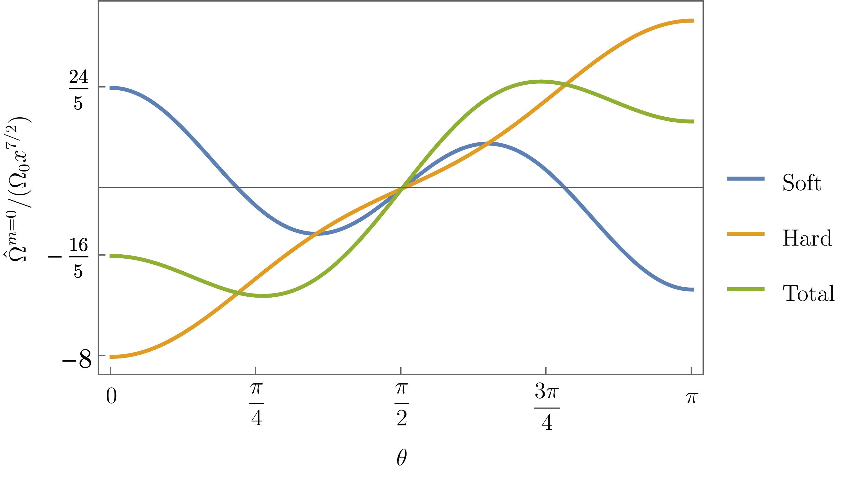
Figure 1: The leading axisymmetric contributions to the precession rate, given in (42) as a function of the polar angle on the celestial sphere (with respect to the axis of rotation of the binary). The leading memory effects have similar angular dependence, see (43).

This equation shows the accumulated memory effect from an initial time $u_{0}$ at which $x(u_{0})=x_{0}$, to the current time $u$ with $x=x(u)$. Given that the quasi-circular model breaks down after the innermost stable circular orbit (ISCO), one has to restrict to the regime where $x<x_{\text{ISCO}}=\tfrac{1}{6}$. On the other hand, the quasi circular model cannot be extended to the far past. They are rather formed over time through mechanisms such as dynamic capture, or the fragmentation of astrophysical clouds. Here, we think of a quasi-circular orbit as the solution to an initial value problem, where the binary is circular at in initial time $u_{0}$. Moreover, note that the Blanchet-Damour formalism typically assumes a “past-stationarity” condition, i.e. , that gravitational fields are stationary before an initial time $u<u_{0}$. A more careful analysis of IR divergences may be dealt with in a scattering setup, see e.g. [49, 50] for related works. In this sense, $0<x_{0}\ll 1$ can be thought of as an infrared cutoff.

5 Concluding remarks

Let us briefly summarize and point out some future directions, which we plan to explore. We showed that gravitational waves from a binary system lead to a small change in the orientation of a distant gyroscope. In [22], we estimated the effect to be proportional to $\frac{G^{2}M^{2}}{r^{2}c^{4}}$, based on a dimensional analysis. We observe that the dimensional analysis captures most of the result in (43), except the dimensionless accumulation factor $\left(\frac{1}{\sqrt{x}}-\frac{1}{\sqrt{x_{0}}}\right)$ and the dimensionless symmetric mass ratio $\nu$. If the gyroscope is subject to long-lasting GW signal, the accumulation effect can lead to a large enhancement. At the same time, we note that the result is suppressed for extreme mass-ratio inspirals, for which $\nu\ll 1$. Overall, the result is still very small, and unlikely to be observed in a realistic experiment.

In this paper, we have focused on the effect of GWs on a single gyroscope. An alternative scenario is to measure the effect on a large set of gyroscopes distributed on the celestial sphere. For example, one can think of pulsars surrounding a binary system. Accordingly, one can study the correlation among the gyroscopes, and contrast it with the result (43) in this paper.

Another interesting issue is to study more carefully the gyroscopic memory when the the test gyroscope is highly spinning. In this case, the parallel transport approximation is not suitable, and one has to consider higher-order effects described in section 2. These could be of relevance for highly spinning neutron stars as probes of GWs.

Appendix A Spin weighted functions on sphere

Consider a null dyad $m^{A},{\overline{m}}^{A}$ on a two-dimensional sphere such that $m^{A}m_{A}=0={\overline{m}}^{A}{\overline{m}}_{A}$ and $m^{A}{\overline{m}}_{A}=1$. Inverting these relations allows finding the expression (11) of $m_{A}{\overline{m}}_{B}$ in terms of the tensors $\gamma_{AB}$, $\varepsilon_{AB}$. Under a $U(1)$ rotation in the tangent space of a given point on the sphere, the dyad transforms as

$$m^{A}\to{\rm e}^{{\rm i}\mskip 1.5mu\theta}m^{A}\,,\qquad{\overline{m}}\to{\rm e}^{-{\rm i}\mskip 1.5mu\theta}\,{\overline{m}}\,.$$ (44)

Given a tensor $T$ of rank $p+q$, one can construct spin-weighted functions by contraction with basis vectors $m^{A}$ and ${\overline{m}}^{A}$, e.g.,

$$T_{s} \equiv T_{A_{1}\cdots A_{p}B_{1}\cdots B_{q}}m^{A_{1}}\cdots m^{A_{p}}{\overline{m}}^{B_{1}}\cdots{\overline{m}}^{B_{q}}$$ (45)

with $p$ factors of $m^{A}$ and $q$ factors of ${\overline{m}}^{A}$. The complex function $T_{s}$ has spin-weight $s=p-q$, as it transforms under dyad rotations as $T_{s}\to{\rm e}^{{\rm i}s\mskip 1.5mu\theta}T_{s}$. We note that using (11) in (45), we can trade mutual factors $m^{A}$, ${\overline{m}}^{A}$ for the metric and the epsilon tensor. Accordingly, the tensor $T$ in (45) is reduced into its irreducible representations under the rotation group. In particular, a symmetric trace-free (STF) tensor $\hat{T}$ on the sphere has only two degrees of freedom, which are encoded in a single complex function $\mathcal{T}_{s}=\hat{T}_{A_{1}\cdots A_{s}}m^{A_{1}}\cdots m^{A_{s}}$. (The function of a spin weight $-s$ function obtained by contracting all indices with factors of ${\overline{m}}^{B}$ is not independent, as they are complex conjugates.).

In this language, covariant derivatives acting on tensors on the sphere are replaced by the so-called eth $\eth$ derivative and its conjugate ${\overline{\eth}}$ acting on spin-weighted functions as

$$\eth T_{s} =m^{A_{1}}\cdots m^{A_{p}}{\overline{m}}^{B_{1}}\cdots{\overline{m}}^{B_{q}}m^{C}\mathrm{D}_{C}T_{A_{1}\cdots A_{p}B_{1}\cdots B_{q}}\,,$$ (46)

while ${\overline{\eth}}T_{s}$ is defined by conjugating the vector that contracts with the derivative, i.e. , $m^{C}\to{\overline{m}}^{C}$ in the above equation. By construction, $\eth({\overline{\eth}})$ increases (decreases) the spin-weight by $+1$ $(-1)$.

Spin-weighted harmonics

Spin-weighted harmonics ${{}_{s}{Y}^{\ell m}}$ provide a basis for spin-weighted functions on the sphere. They are defined in terms of standard harmonics $Y^{\ell m}\equiv{{}_{0}{Y}^{\ell m}}$. For a positive integer $s$,

$${{}_{s}{Y}^{\ell m}} \equiv(-\sqrt{2})^{s}\sqrt{\frac{(\ell-s)!}{(\ell+s)!}}\;\eth^{s}Y^{\ell m}\,,\qquad{{}_{-s}{Y}^{\ell m}}\equiv(\sqrt{2})^{s}\sqrt{\frac{(\ell-s)!}{(\ell+s)!}}\;{\overline{\eth}}^{s}Y^{\ell m}\,.$$ (47)

and the spin-weighted harmonics vanish when $|s|>\ell$. The definition implies several important properties of spin-weighted harmonics. Under conjugation

$${{}_{s}{\overline{Y}}^{\ell m}}=(-1)^{m+s}{{}_{-s}{Y}^{\ell-m}}\,.$$ (48)

Moreover, for any non-negative $s\leqslant\ell$,

$$\eth\,{{}_{s}{Y}^{\ell m}} =-\sqrt{\frac{(\ell-s)(\ell+s+1)}{2}}{{}_{s+1}{Y}^{\ell m}}\,,\quad{\overline{\eth}}\,{{}_{s}{Y}^{\ell m}}=\sqrt{\frac{(\ell+s)(\ell-s+1)}{2}}{{}_{s-1}{Y}^{\ell m}}\,.$$ (49a)

Finally, as a complete basis, the obey orthogonality relations given in terms of the $3j$ symbols

$$\int_{S^{2}}\text{d}^{2}\mathit{\Omega}\;{{}_{s}{Y}^{\ell_{1}m_{1}}}\,{{}_{s}{\overline{Y}}^{\ell_{2}m_{2}}}=\delta_{\ell_{1}\ell_{2}}\delta_{m_{1}m_{2}}$$ (50a)

$$\int_{S^{2}}\text{d}^{2}\mathit{\Omega}\;{{}_{s_{1}}{Y}^{\ell_{1}m_{1}}}\,{{}_{s_{2}}{Y}^{\ell_{2}m_{2}}}\,{{}_{s}{Y}^{\ell m}}$$

$$\qquad\qquad=\sqrt{\frac{(2\ell_{1}+1)(2\ell_{2}+1)(2\ell+1)}{4\pi}}\begin{pmatrix}\ell_{1}&\ell_{2}&\ell\\ m_{1}&m_{2}&m\end{pmatrix}\begin{pmatrix}\ell_{1}&\ell_{2}&\ell\\ -s_{1}&-s_{2}&-s\end{pmatrix}\,.$$ (50b)

Appendix B Review of the PN/PM formalism

To investigate the dynamics of isolated systems of ordinary matter in general relativity, we must resort to approximation methods adapted to the situation we are interested in. In the case where the typical velocities of the problem are all significantly smaller than the speed $c$ of light in some portion of spacetime, we may use the post-Newtonian expansion, a perturbative scheme with small parameter $\varepsilon=v/c$, where $v$ is the largest of those velocities. As a result, this perturbative expansion is valid in a region of spacetime around the source, whose size is small compared to the wavelength $\lambda$ of the emitted gravitational radiation, usually referred to as the system’s near zone.

By contrast, the post-Minkowskian (PM) formalism is a perturbative expansion in which the small quantity is the magnitude of the field perturbation relative to the flat spacetime, with the gravitational constant $G$ serving as a book-keeping parameter. The approximation may be employed to compute the gravitational field on distances comparable to or larger than $\lambda$ without further restriction. Moreover, outside the matter distribution, the so-called exterior zone, it is particularly convenient to construct the most general post-Minkowskian solution of Einstein’s equations in the form of a multipole expansion. This approach is referred to as the multipolar post-Minkowskian (MPM) formalism. The MPM expansion can be combined with the post-Newtonian scheme using the method of matched asymptotic expansions [51], thanks to an overlap between the near zone and the exterior zone in which the two expansions are valid. This provides a powerful setup to compute the gravitational waves produced by the source under consideration (see [52] for a detailed review).

It is convenient, in this framework, to represent the gravitational field as the gothic metric deviation $h^{{\mu\nu}}=\sqrt{-g}g^{\mu\nu}-\eta^{{\mu\nu}}$ from a background Minkowski metric $\eta_{{\mu\nu}}$, where $g$ denotes the determinant of $g_{{\mu\nu}}$ in a Minkowskian frame, and impose the harmonic gauge condition $\partial_{\nu}h^{{\mu\nu}}=0$. The remaining “relaxed” Einstein equations then read

$$\Box h^{{\mu\nu}}=\frac{16\pi G}{c^{4}}\tau^{{\mu\nu}}\,,$$ (51)

with $\Box$ representing the flat d’Alembertian operator. The pseudo stress-energy tensor $\tau^{{\mu\nu}}=|g|T^{{\mu\nu}}+c^{4}\Lambda^{{\mu\nu}}[h]/(16\pi G)$ entering the right-hand side is made of a matter contribution proportional to the stress-energy tensor $T^{{\mu\nu}}$, with compact support, supplemented by all nonlinear terms, at least quadratic in $h^{{\mu\nu}}$ and its derivatives.

The formal post-Newtonian solution $\overline{h}^{{\mu\nu}}$ of (51), valid in the near zone, may be obtained as [53, 54]

$$\mathop{\overline{h}}\!{}^{{\mu\nu}} =\frac{16\pi G}{c^{4}}\,\mathop{\text{FP}}_{B=0}\Box^{-1}_{\text{R}}\bigg{[}\left(\frac{r}{r_{0}}\right)^{\!B}\mathop{\overline{\tau}}\!{}^{{\mu\nu}}\bigg{]}$$

$$-\frac{4G}{c^{4}}\sum^{+\infty}_{\ell=0}\frac{(-1)^{\ell}}{\ell!}\hat{\partial}_{L}\bigg{\{}\frac{\overline{{\cal R}_{L}^{{\mu\nu}}(t-r/c)-{\cal R}_{L}^{{\mu\nu}}(t+r/c)}}{2r}\bigg{\}}\,.$$ (52)

The first term on the right-hand side is a particular solution, obtained in three steps: (1) We multiply the integrand by a kernel function $(r/r_{0})^{B}$, where $r_{0}$ is cut-off length. (2) We apply the retarded integral operator, yielding a result that may be regarded as a function of $B$, say $F(B)$, the spacetime dependence being implicit here. (3) We extract the finite part of $F(B)$ at $B=0$, i.e. , the term proportional to $B^{0}$ in the Laurent expansion of $F$ near $B=0$, as indicated by the operator $\text{FP}_{B=0}$. The second term is a smooth homogeneous solution, which is undetermined in a first stage.

In the exterior zone, the stress-energy tensor $T^{{\mu\nu}}$ vanishes. The various orders composing the MPM gravitational field $\mathcal{M}(h^{{\mu\nu}})=\sum_{n\geqslant 1}G^{n}h_{n}^{{\mu\nu}}$ are computed iteratively from the linear vacuum solution. The most general solution of the relaxed Einstein field equations $\Box h_{1}^{{\mu\nu}}=0$ is an infinite sum of space derivatives of retarded spherical waves,

$$Gh^{{\mu\nu}}_{1} =-\frac{4G}{c^{4}}\sum_{\ell=0}^{+\infty}\frac{(-1)^{\ell}}{\ell!}\partial_{L}\left(\frac{\mathcal{H}^{\mu\nu}_{L}(t-r/c)}{r}\right)_{,}.$$ (53)

where the $\mathcal{H}^{\mu\nu}_{L}(u)$ are arbitrary functions of the retarded time $u=t-r/c$. Without any loss of generality, we may assume that those tensors are STF over the multi-index $L$. After imposing the harmonicity condition $\partial_{\nu}h^{{\mu\nu}}=0$, we find that $Gh_{1}^{{\mu\nu}}=Gh^{\mu\nu}_{\text{can}\,1}[I_{L},J_{L}]+(\partial\xi)^{\mu\nu}$, where the canonical solution $h^{\mu\nu}_{\text{can}\,1}[I_{L},J_{L}]$ depends on source mass moments $I_{L}$ (with $\ell\geqslant 0$) and source current moments $J_{L}$ (with $\ell\geqslant 1$), while the linear gauge transformation $(\partial\xi)^{\mu\nu}$ is a function of four sets of STF gauge multipole moments, namely $W_{L}$, $X_{L}$, $Y_{L}$ and $Z_{L}$ [44, 55]. Note that $I$ is nothing but the conserved (Arnowitt-Deser-Misner [56]) mass of the system, $\dot{I}_{i}$ the conserved linear momentum, and $J_{i}$ the conserved angular momentum.

If the orders $m<n$ are known, it is straightforward to form the source $\Lambda^{\mu\nu}_{n}$ of the relaxed Einstein field equation for $h_{n}^{\mu\nu}$, which can thus be written as

$$\Box h_{n}^{\mu\nu}=\Lambda^{\mu\nu}_{n}\,.$$ (54)

In particular, due to the gauge condition, $\Lambda^{\mu\nu}_{n}$ must be divergence free. Applying the operator $FP_{B=0}\Box^{-1}_{R}[(r/r_{0})^{B}~{}]$, introduced earlier to solve the near zone equations, on both sides of (54) yields $h^{{\mu\nu}}_{n}=u^{\mu\nu}_{n}+v^{\mu\nu}_{n}$, where $u^{\mu\nu}_{n}=FP_{B=0}\Box^{-1}_{R}[(r/r_{0})^{B}\Lambda^{\mu\nu}_{n}]$ and $v_{n}^{\mu\nu}$ is an unspecified homogeneous solution. Since the divergence of $h^{\mu\nu}_{n}$ has to vanish, $v^{\mu\nu}$ is also bound to satisfy $\partial_{\nu}v_{n}^{\mu\nu}=-\partial_{\nu}u_{n}^{{\mu\nu}}$. The vector $w_{n}^{\mu}\equiv\partial_{\nu}u_{n}^{{\mu\nu}}$, as a solution of the vacuum wave equation, can be decomposed into irreducible STF multipole moments in form similar to (53) (with one less index). Now, from any vector $w^{\mu}$ written in this way, there exists an algorithm to build a tensor $\mathcal{H}^{\mu\nu}[w^{\alpha}]$ such that $\partial_{\nu}\mathcal{H}^{\mu\nu}=-w^{\mu}$. The most general solution is thus finally given by $h_{n}^{\mu\nu}=u^{{\mu\nu}}_{n}+\mathcal{H}^{\mu\nu}[w^{\alpha}_{n}]$, with $w_{n}^{\mu}=\partial_{\nu}u^{{\mu\nu}}_{n}$. Any residual freedom in the solution $h_{n}^{\mu\nu}$ obeys the linear vacuum Einstein equations, so that they can be absorbed by an appropriate redefinition of the source and gauge moments.

Given the near-zone PN solution $\overline{h}^{\mu\nu}$ and the exterior zone MPM solution $\mathcal{M}(h^{\mu\nu})$, the function $\mathcal{R}^{\mu\nu}_{L}(t)$ and the source multipole moments are determined by imposing that $\overline{h}^{\mu\nu}$ and $\mathcal{M}(h^{\mu\nu})$ coincide in their common domain of validity, i.e. the matching condition

$$\overline{\mathcal{M}(h)}=\mathcal{M}(\overline{h}^{\mu\nu})\,$$ (55)

holds in this “buffer” zone [57, 53]. This provides explicit general formulae for the homogeneous solution in Eq. (B), as well as the multipole moments, which can be found in dedicated references, such as the review article [43].

Appendix C Time integration and memory effect

To compute the leading order contribution to the gyroscopic memory, we need to integrate the precession rates (4.3), (41) over time. These integrals take the form

$$I_{\alpha,m}(u)=\int_{-\infty}^{u}\text{d}t\,x(t)^{\alpha}\,{\rm e}^{{\rm i}\mskip 1.5mum\mskip 1.5mu\varphi(t)}\,.$$ (56)

Note that $x(t)$ is an adiabatic variable, while $\phi(t)$ is a fast oscillatory variable. Therefore the case $m=0$ in (56) is a special case which reads

$$I_{\alpha,0}(u)=\int_{-\infty}^{u}\text{d}t\,x^{\alpha}=\int_{-\infty}^{u}\text{d}x\,\frac{x^{\alpha}}{\dot{x}}$$ (57)

The time evolution of $x$ is obtained by the flux-balance equation for energy [46], implying that

$$\dot{x} =\frac{64}{5}\frac{c^{3}\nu}{GM}\,x^{5}\,\Big{(}1+\mathcal{O}\Big{(}\frac{1}{c^{2}}\Big{)}\Big{)}$$ (58)

This equation can be used in (57) to compute the time integral of axisymmetric modes

$$I_{\alpha,0}(u) =\frac{5}{64}\frac{GM}{c^{3}\nu}\frac{1}{\alpha-4}x^{\alpha-4}\Big{(}1+\mathcal{O}\Big{(}\frac{1}{c^{2}}\Big{)}\Big{)}\,, \alpha \neq 4\,.$$ (59)

On the other hand, the case $m\neq 0$ can be processed by the following replacement in (56)

$$e^{{\rm i}m\varphi}=\frac{1}{{\rm i}m}\frac{\partial}{\partial\varphi}e^{{\rm i}m\varphi}=\frac{1}{{\rm i}m\omega}\frac{\partial}{\partial t}e^{{\rm i}m\varphi}=\frac{GM}{c^{3}}\frac{x^{-3/2}}{{\rm i}m}\frac{\partial}{\partial t}e^{{\rm i}m\varphi}\,,$$

and performing integration by parts to move time derivatives from the fast variable to the slow variable. We thus find

$$I_{\alpha,m}(u) =\frac{GM}{c^{3}}\frac{1}{{\rm i}m}\left[x^{\alpha-3/2}e^{{\rm i}m\varphi}\Big{|}_{-\infty}^{u}-\int_{-\infty}^{u}\text{d}te^{{\rm i}m\varphi}\frac{\text{d}}{\text{d}t}\big{(}x^{\alpha-3/2}\big{)}\right]\,.$$ (60)

Assuming that $\alpha>3/2$, the first term vanishes at the lower bound and the integral localizes to an instantaneous expression (this does not hold for $\alpha=3/2$ which we come back to later). Moreover, using (58), the integrand of the integral in (60) is $\text{d}(x^{\alpha-3/2})/\text{d}t=(\alpha-3/2)(64/5)(c^{3}\nu)/(GM)\,x^{\alpha+5/2}$, and the integral takes the same form as (56). We can therefore repeat the above algorithm, which implies

$$I_{\alpha,m}(u) =\frac{GM}{c^{3}}\frac{{\rm e}^{{\rm i}m\mskip 1.5mu\varphi(u)}}{{\rm i}m}x(u)^{\alpha-3/2}\left[1-(\alpha-3/2)\frac{64}{5}\frac{\nu}{{\rm i}m}x^{5/2}+\cdots\right]\,,~{}\alpha>\frac{3}{2},~{}m\neq 0\,.$$ (61)

We observe that the result is a perturbative PN expansion, where the first correction is 2.5PN subleading with respect to the leading term. Therefore, for the purpose of our work, only the leading term is sufficient. Subleading terms can be found by repeating the above procedure to reach the desired order.

For $\alpha\leqslant 4$ in (59) and $\alpha\leqslant 3/2$ in (61), the integrals are not convergent. However, the quasi-circular orbit cannot be trusted in the far past, as we discussed below (43). Therefore, we regulate the integrals by modifying the lower bound from $-\infty$ to $u_{0}$, which can be a large but finite negative constant.

References

- [1] C. W. Misner, K. S. Thorne and J. A. Wheeler, Gravitation. W. H. Freeman, San Francisco, 1973.
- [2] R. Brito, V. Cardoso and P. Pani, Superradiance: New Frontiers in Black Hole Physics, Lect. Notes Phys. 906 (2015) pp.1–237 [1501.06570].
- [3] R. D. Blandford and R. L. Znajek, Electromagnetic extractions of energy from Kerr black holes, Mon. Not. Roy. Astron. Soc. 179 (1977) 433–456.
- [4] M. Mathisson, Neue mechanik materieller systemes, Acta Phys. Polon. 6 (1937) 163–200.
- [5] A. Papapetrou, Spinning test-particles in general relativity. i, Proceedings of the Royal Society of London. Series A. Mathematical and Physical Sciences 209 (1951), no. 1097 248–258.
- [6] W. Tulczyjew, Equations of motion of rotating bodies in general relativity theory, Acta Phys. Polon 18 (1959) 37.
- [7] W. G. Dixon, Dynamics of extended bodies in general relativity. i. momentum and angular momentum, Proceedings of the Royal Society of London. A. Mathematical and Physical Sciences 314 (1970), no. 1519 499–527.
- [8] W. G. Dixon, Dynamics of extended bodies in general relativity. II. Moments of the charge-current vector, Proc. Roy. Soc. Lond. A 319 (1970) 509–547.
- [9] W. G. Dixon, Dynamics of extended bodies in general relativity III. Equations of motion, Phil. Trans. Roy. Soc. Lond. A 277 (1974), no. 1264 59–119.
- [10] I. Bailey and W. Israel, Lagrangian Dynamics of Spinning Particles and Polarized Media in General Relativity, Commun. Math. Phys. 42 (1975) 65–82.
- [11] H. Tagoshi, A. Ohashi and B. J. Owen, Gravitational field and equations of motion of spinning compact binaries to 2.5 postNewtonian order, Phys. Rev. D 63 (2001) 044006 [gr-qc/0010014].
- [12] G. Faye, L. Blanchet and A. Buonanno, Higher-order spin effects in the dynamics of compact binaries. I. Equations of motion, Phys. Rev. D 74 (2006) 104033 [gr-qc/0605139].
- [13] R. A. Porto, The effective field theorist’s approach to gravitational dynamics, Phys. Rept. 633 (2016) 1–104 [1601.04914].
- [14] M. Levi and J. Steinhoff, Spinning gravitating objects in the effective field theory in the post-Newtonian scheme, J. High Energy Phys. 2015 (2015), no. 09 [1501.04956].
- [15] E. E. Flanagan, A. M. Grant, A. I. Harte and D. A. Nichols, Persistent gravitational wave observables: general framework, Phys. Rev. D99 (2019), no. 8 084044 [1901.00021].
- [16] Y. B. Zel’dovich and A. G. Polnarev, Radiation of gravitational waves by a cluster of superdense stars, Sov.Astron. 18 (1974) 17.
- [17] V. B. Braginsky and L. P. Grishchuk, Kinematic Resonance and Memory Effect in Free Mass Gravitational Antennas, Sov. Phys. JETP 62 (1985) 427–430.
- [18] V. B. Braginsky and K. S. Thorne, Gravitational-wave bursts with memory and experimental prospects, Nature 327 (1987), no. 6118 123–125.
- [19] D. Christodoulou, Nonlinear nature of gravitation and gravitational wave experiments, Phys. Rev. Lett. 67 (1991) 1486–1489.
- [20] L. Blanchet and T. Damour, Hereditary effects in gravitational radiation, Phys. Rev. D46 (1992) 4304–4319.
- [21] A. Seraj and B. Oblak, Gyroscopic gravitational memory, JHEP 11 (2023) 057 [2112.04535].
- [22] A. Seraj and B. Oblak, Precession Caused by Gravitational Waves, Phys. Rev. Lett. 129 (2022), no. 6 061101 [2203.16216].
- [23] E. Corinaldesi and A. Papapetrou, Spinning test particles in general relativity. 2., Proc. Roy. Soc. Lond. A 209 (1951) 259–268.
- [24] B. M. Barker and R. F. Oconnell, The gravitational interaction: spin, rotation, and quantum effects - a review., General Relativity and Gravitation 11 (Oct., 1979) 149–175.
- [25] L. F. O. Costa and J. Natário, Center of mass, spin supplementary conditions, and the momentum of spinning particles, Fund. Theor. Phys. 179 (2015) 215–258 [1410.6443].
- [26] W. G. Dixon, A covariant multipole formalism for extended test bodies in general relativity, Nuovo Cim. 34 (1964), no. 2 317–339.
- [27] S. Marsat, Cubic order spin effects in the dynamics and gravitational wave energy flux of compact object binaries, Class. Quant. Grav. 32 (2015), no. 8 085008 [1411.4118].
- [28] W. D. Goldberger and I. Z. Rothstein, An Effective field theory of gravity for extended objects, Phys. Rev. D73 (2006) 104029 [hep-th/0409156].
- [29] L. Freidel, R. Oliveri, D. Pranzetti and S. Speziale, The Weyl BMS group and Einstein’s equations, JHEP 07 (2021) 170 [2104.05793].
- [30] M. Godazgar, G. Macaulay, G. Long and A. Seraj, Gravitational memory effects and higher derivative actions, JHEP 09 (2022) 150 [2206.12339].
- [31] A. Seraj and T. Neogi, Memory effects from holonomies, Phys. Rev. D 107 (2023), no. 10 104034 [2206.14110].
- [32] S. Pasterski, A. Strominger and A. Zhiboedov, New Gravitational Memories, JHEP 12 (2016) 053 [1502.06120].
- [33] D. A. Nichols, Spin memory effect for compact binaries in the post-Newtonian approximation, Phys. Rev. D95 (2017), no. 8 084048 [1702.03300].
- [34] G. Compère, R. Oliveri and A. Seraj, The Poincaré and BMS flux-balance laws with application to binary systems, JHEP 10 (2020) 116 [1912.03164].
- [35] K. Mitman, J. Moxon, M. A. Scheel, S. A. Teukolsky, N. Deppe, L. E. Kidder and W. Throwe, Computation of Normal and Spin Memory in Numerical Relativity, 2007.11562.
- [36] A. Maleknejad, Photon chiral memory effect stored on celestial sphere, JHEP 06 (2023) 193 [2304.05381].
- [37] W.-B. Liu, J. Long and X.-H. Zhou, Electromagnetic helicity flux operators in higher dimensions, 2407.20077.
- [38] J. Dong, J. Long and R.-Z. Yu, Gravitational helicity flux density from two-body systems, 2403.18627.
- [39] U. Kol, Duality in Einstein’s Gravity, 2205.05752.
- [40] V. Hosseinzadeh, A. Seraj and M. M. Sheikh-Jabbari, Soft Charges and Electric-Magnetic Duality, JHEP 08 (2018) 102 [1806.01901].
- [41] I. M. Gelfand, R. A. Minlos, Z. Y. Shapiro, G. Cummins and T. Boddington, Representations of the rotation and lorentz groups and their applications, (No Title) (1963).
- [42] E. T. Newman and R. Penrose, Note on the Bondi-Metzner-Sachs group, J. Math. Phys. 7 (1966) 863–870.
- [43] L. Blanchet, Gravitational Radiation from Post-Newtonian Sources and Inspiralling Compact Binaries, Living Rev. Rel. 17 (2014) 2 [1310.1528].
- [44] K. S. Thorne, Multipole Expansions of Gravitational Radiation, Rev. Mod. Phys. 52 (1980) 299–339.
- [45] G. Faye, S. Marsat, L. Blanchet and B. R. Iyer, The third and a half post-Newtonian gravitational wave quadrupole mode for quasi-circular inspiralling compact binaries, Class. Quant. Grav. 29 (2012) 175004 [1204.1043].
- [46] L. Landau and E. Lifshitz, The classical theory of fields. Pergamon, Oxford, 1971.
- [47] L. Blanchet, G. Faye, Q. Henry, F. Larrouturou and D. Trestini, Gravitational-wave flux and quadrupole modes from quasicircular nonspinning compact binaries to the fourth post-Newtonian order, Phys. Rev. D 108 (2023), no. 6 064041 [2304.11186].
- [48] L. Blanchet, T. Damour, G. Esposito-Farèse and B. R. Iyer, Gravitational radiation from inspiralling compact binaries completed at the third post-newtonian order, Phys. Rev. Lett. 93 (2004) 091101 [gr-qc/0406012].
- [49] B. Sahoo and A. Sen, Classical and Quantum Results on Logarithmic Terms in the Soft Theorem in Four Dimensions, JHEP 02 (2019) 086 [1808.03288].
- [50] L. Kehrberger, Mathematical Studies on the Asymptotic Behaviour of Gravitational Radiation in General Relativity. PhD thesis, Department of Applied Mathematics And Theoretical Physics, Cambridge U., 2023.
- [51] E. J. Hinch, Perturbation Methods, vol. 6 of Cambridge Texts in Applied Mathematics. Cambridge University Press, 1991.
- [52] L. Blanchet, Post-Newtonian theory for gravitational waves, Living Rev. Relativ. 27 (2024) 4 [arXiv:1310.1528].
- [53] O. Poujade and L. Blanchet, Post-Newtonian approximation for isolated systems calculated by matched asymptotic expansions, Phys. Rev. D 65 (2002) 124020 [gr-qc/0112057].
- [54] L. Blanchet, G. Faye and S. Nissanke, Structure of the post-newtonian expansion in general relativity, Phys. Rev. D 72 (2005) 044024.
- [55] L. Blanchet and T. Damour, Radiative gravitational fields in general relativity I. general structure of the field outside the source, Phil. Trans. Roy. Soc. Lond. A320 (1986) 379–430.
- [56] R. L. Arnowitt, S. Deser and C. W. Misner, Dynamical Structure and Definition of Energy in General Relativity, Phys. Rev. 116 (1959) 1322–1330.
- [57] L. Blanchet, On the multipole expansion of the gravitational field, Class. Quant. Grav. 15 (1998) 1971–1999 [gr-qc/9801101].