Chebyshev polynomials related to Jacobi weights
Abstract.
We investigate Chebyshev polynomials corresponding to Jacobi weights and determine monotonicity properties of their related Widom factors. This complements work by Bernstein from 1930-31 where the asymptotical behavior of the related Chebyshev norms was established. As a part of the proof, we analyze a Bernstein-type inequality for Jacobi polynomials due to Chow et al. Our findings shed new light on the asymptotical uniform bounds of Jacobi polynomials. We also show a relation between weighted Chebyshev polynomials on the unit circle and Jacobi weighted Chebyshev polynomials on . This generalizes work by Lachance et al. In order to complete the picture we provide numerical experiments on the remaining cases that our proof does not cover.
Keywords Chebyshev polynomial, Widom factor, Jacobi weight, Jacobi polynomial, Bernstein-type inequality
Mathematics Subject Classification 41A50. 30C10. 33C45.
1. Introduction
In an extensive two part analysis of extremal polynomials on the unit interval, found in [8, 9], S. N. Bernstein investigates the asymptotic behavior of the quantity
| (1.1) |
as for a variety of different conditions on the weight function . If is bounded and strictly positive on a set consisting of at least points on , there exists a unique set of nodes , all situated in , such that
| (1.2) |
see for instance [1, 33, 40]. In other words, the infimum of (1.1) can be replaced by a minimum. The polynomial
| (1.3) |
is the weighted Chebyshev polynomial of degree corresponding to the weight function and it is the unique monic polynomial of degree minimizing (1.1). Under the assumption that the weight function is continuous, the minimizer of (1.1) can be characterized by the so-called alternation property. That is to say, a monic polynomial of degree is equal to (and thus minimizes (1.1)) if and only if there exists points such that
| (1.4) |
This result – which is central to the study of best approximations on the real line – can be found in many works on approximation theory, see for instance [33, 1, 14, 37].
The study of (1.1) dates back to the work of P. L. Chebyshev [10, 11] who considered weight functions of the form where is a polynomial which is strictly positive on the interval . Later A. A. Markov [35] extended these results to allow for weight functions of the form , where again is a polynomial which is assumed to be strictly positive on . It should be stressed that both Chebyshev and Markov provided explicit formulas for the minimizer in these cases in terms of the polynomial . These formulas can be conveniently found in Achiezer’s monograph [1, Appendix A].
The considerations in [8, 9] were different from those of Chebyshev and Markov as Bernstein considered the asymptotic behavior of (1.1) as for a broad family of weights, not restricting himself to continuous ones. In particular, writing as if as , he obtained the following result.
Theorem 1.1 (Bernstein [9]).
Let and for , and let be a Riemann integrable function such that there exists a value for which holds for every . Consider the weight function given by
Under the above conditions, we have that
| (1.5) |
as .
This result is shown in two steps. Bernstein initially considers weight functions as in Theorem 1.1 and finds that if are the unique nodes satisfying
| (1.6) |
then the weighted expression
is asymptotically alternating on , see [8]. As it turns out, this information suffices to apply a result due to de la Vallée-Poussin found in [18] and ensure that
| (1.7) |
as . Note that
is nothing but the monic orthogonal polynomial of degree corresponding to the weight function on . By showing that
as , Bernstein obtains (1.5) from (1.7). Consequently, Theorem 1.1 is verified in this case. Proceeding from this, Bernstein extends the analysis by allowing for vanishing factors of the form to be introduced to the weight where and , see [9]. To show this, he uses a clever technique of bounding the factors from above and below. However, the connection to the maximal deviation of the corresponding orthogonal polynomials as in (1.7) gets lost.
To illustrate why this connection becomes more delicate when zeros are added to the weight function, he provides the explicit example of the monic Jacobi polynomials. Following [41, Chapter IV], we let denote the classical Jacobi polynomials with parameters These are uniquely defined by the property that is a polynomial of exact degree and
| (1.8) |
where is the Kronecker delta. Since all zeros of the Jacobi polynomials reside in and since
we find that
| (1.9) |
for some values . Bernstein’s analysis provides the following result.
Theorem 1.2 (Bernstein [9]).
Note that by replacing with in (1.6), the corresponding weight function, to which the orthogonal polynomials are associated, is nothing but
| (1.12) |
It is a simple matter to verify that
| (1.13) |
see for instance [13] where also a translation of the proof of Theorem 1.1 appears. As such, we see that the monic Jacobi polynomials defined in (1.9) are close to minimal with respect to
| (1.14) |
precisely when (1.10) holds.
As a partial result, we wish to carry out a detailed analysis of the quantity
for the parameters satisfying (1.10). By carefully manipulating a Bernstein-type inequality due to Chow et al. [12], we will establish the following result.
Theorem 1.3.
By combining Theorem 1.3 with Theorem 1.2, we see that
| (1.16) | ||||
which shows that the convergence is from below. The question of obtaining upper bounds for the quantity
| (1.17) |
for different values of is well studied, see for instance [19, 12, 27] and has applications to e.g. representation theory and the study of Schrödinger operators. Our main interest is the applications that such a result has to the corresponding Chebyshev problem (1.14). To state our main result, we introduce the Widom factor defined by
| (1.18) |
The choice of naming in honour of H. Widom – who in [44] considered Chebyshev polynomials corresponding to a plethora of compact sets in the complex plane – stems from [24]. The considerations of Widom factors in the literature are plentiful, see for instance [14, 25, 15, 16, 2, 3, 24, 17, 37, 4]. In this article we wish to carry out a detailed study of the behavior of for different parameter values.
Theorem 1.4.
For any value of the parameters , we have that
as . Furthermore:
-
(1)
If , then the quantity is constant.
-
(2)
If , then
(1.19) -
(3)
If , then
(1.20) (1.21) and decreases monotonically as increases.
The case of is classical and if and (or vice versa), the result was settled in [7]. We will in fact apply a similar technique to what is used there for the general setting of . This method originates with [30]. As such, the proofs of the different cases of Theorem 1.4 uses essentially different techniques and will be split into three separate sections.
We should also note that while negative parameters and are allowed in Theorem 1.1, they simply result in the fact that a zero of the minimizer is forcedly placed to cancel the effect of the pole and hence the setting transfers to the one of non-negative parameters if the degree of the associated Chebyshev polynomial is sufficiently large.
Asymptotic results for the Chebyshev polynomials corresponding to (1.1) exist for smooth enough weight functions which are strictly positive on . See for instance [34, 29, 28]. If the weight function vanishes somewhere on , there does not seem to be many general results for the corresponding Chebyshev polynomials apart from Theorem 1.1 found in [9].
The extension of Chebyshev polynomials to the complex plane was first carried out by Faber in [20]. Apart from the proof of Theorem 4.3, our considerations exclusively concern Chebyshev polynomials corresponding to Jacobi weights and we therefore refrain from a detailed presentation of the general complex case. We note, however, that if is a compact set and is a weight function which is non-zero for at least points, then there exists a unique monic polynomial of degree minimizing
We invite the reader to consult [40, 37] for a detailed presentation of complex Chebyshev polynomials.
Our motivation in providing a detailed study of originates from an inquiry of complex Chebyshev polynomials corresponding to star graphs of the form . It can be shown that these complex Chebyshev polynomials can be directly related to Chebyshev polynomials on with Jacobi weights, see [13] for details. In the study of the Widom factors for star graphs, certain monotonicity properties appear which can be explained by Theorem 1.4. We trust that Theorem 1.4 will also be useful in many other connections.
2. The case of
We proceed by delving into the proof of Theorem 1.4, split into three cases. The first case is very simple. When , the minimizers of (1.18) are simply the Chebyshev polynomials of the 1 to 4 kind, see e.g. [36]. Using basic trigonometry, it follows that if then
| (2.1) | ||||
| (2.2) |
Through the change of variables , the trigonometric functions
all define monic polynomials in of degree . These are precisely, in order, the monic Chebyshev polynomials of the 1, 2, 3 and 4 kind. It is a straightforward matter to verify that they all satisfy the alternating property from (1.4) upon multiplication with the weight functions
respectively. As a result, , and are the minimal configurations sought after in (1.18) for the weight parameters . It is evident that in all these cases and this shows the first part of Theorem 1.4.
3. The case of
Having settled the first case of Theorem 1.4, we turn toward the verification of the second case. For parameter values , we want to show that
| (3.1) |
These parameter values correspond to the lower left square in Figure 1. Observe that if then this follows from the first case of Theorem 1.4 since then the sequence is constant. Our approach will consist of first verifying Theorem 1.3. For this reason we remind the reader of our definition of through the formula
| (3.2) |
where denotes the Jacobi polynomial with parameters and the angles are those for which enumerate its zeros. We also recall the relation between the and parameters
| (3.3) |
If we can show the validity of (1.15), then we trivially obtain
from which (3.1), the second case of Theorem 1.4 follows from the fact that as . The key to verifying (1.15) is the following result.
Theorem 3.1 ([12]).
If and , then
| (3.4) |
where .
This result provides a Bernstein-type inequality for Jacobi polynomials and sharpens a previous result of Baratella [6] who had shown (3.4) with the larger factor in place of . In the case where , the inequality in (3.4) is saturated. For arbitrary the constant is asymptotically sharp as can be seen from an argument using Stirling’s formula which we will provide in the proof of Lemma 3.2. The type of inequality exemplified in (3.4) originate with Bernstein who showed in [9] that the Legendre polynomials satisfy
| (3.5) |
Antonov and Holšhevnikov [5] sharpened (3.5) and later Lorch [32] extended such an inequality to Gegenbauer polynomials. In terms of Jacobi polynomials, this provides a Bernstein-type inequality for with . Theorem 3.1 contains all these inequalities as special cases. In a different direction, the Erdélyi–Magnus–Nevai Conjecture [19] proposes that if denotes the orthonormal Jacobi polynomial then for any parameter values ,
Theorem 3.1 can be used to verify this conjecture in the case where . This is shown in [23] where an extensive consideration concerning the sharpness of Theorem 3.1 is studied numerically for different parameter values.
We consider transferring the trigonometric weights to algebraic weights as in the statement of Theorem 1.3. Letting , we find that
| (3.6) | ||||
| (3.7) |
with the parameter relation stated in (3.3). Together with (3.6), (3.7) and (3.2), the change of variables transforms (3.4) into the statement that for ,
| (3.8) |
where . From (3.3) we see that this implies that
| (3.9) |
for . In order to determine the upper bound of (3.8) and (3.9), we are ultimately led to consider the quantity
| (3.10) |
Lemma 3.2.
Suppose that . Then , defined in (3.10), increases monotonically to as .
The proof we provide constitutes a lengthy computation. We have therefore chosen to illustrate the simpler case where in the proof below while postponing most of the remaining computations to the appendix. The asymptotical behavior as merits attention since this shows that the constant is sharp in (3.4). To see this, note that
The left-hand side converges to as and consequently
On the other hand, as Lemma 3.2 shows, as and therefore the constant factor in (3.4) cannot be improved.
Proof of Lemma 3.2.
We rewrite the binomial coefficients using Gamma functions so that
| (3.11) |
| (3.12) |
The Legendre duplication formula implies that
| (3.13) |
The combination of (3.10), (3.11), (3.12) and (3.13) yields
The Gamma function satisfies that as , and we may conclude that
as .
We are left to determine the monotonicity of . For this reason we consider the quotient
| (3.14) | ||||
Whether this quotient is bigger than or smaller than determines the monotonicity of the sequence . To simplify, we begin by considering the case . Writing , the quotient (3.14) becomes
We introduce the function
and claim that for . From the fact that as , this will imply that for every . As a consequence we see that .
Taking the logarithmic derivative of generates
If , then it is clear that
and as a consequence . We conclude that and this settles the case where .
If , then the problem is more delicate. We again need to show that the quotient (3.14) is strictly greater than . In order to show this, we reintroduce the function by defining it as
| (3.15) |
In a completely analogous manner, we only need to show that for every in order to conclude that and consequently . Since is symmetric with respect to its variables and , it is enough to consider the parameter values .
The logarithmic derivative of is given by
Written over common denominator and utilizing that , this expression becomes
| (3.16) |
where
| (3.17) | ||||
| (3.18) | ||||
| (3.19) |
Now it is immediately clear that unless . We claim that the same is true for the remaining coefficients and . Namely, for unless . A consequence of these inequalities is that for which is precisely the sought after inequality. The proof of this is provided in Lemma 6.1 in the appendix. As a result, we obtain that and therefore
In conclusion, converges monotonically to from below. ∎
An immediate consequence of Lemma 3.2 together with (3.8) is that
| (3.20) |
This simultaneously shows that Theorem 1.3 holds and that
is valid for every . On the other hand, (1.13) implies that these quantities are all asymptotically equal as . This is possible only if
and hence the second case of Theorem 1.4 is shown. From the fact that , we gather the following corollary to Lemma 3.2.
Corollary 3.3.
If and , then
| (3.21) |
and the rightmost inequality is strict unless .
4. The case of
We are left to prove the third and final case of Theorem 1.4. Our approach to proving this revolves around relating Jacobi weighted Chebyshev polynomials to weighted Chebyshev polynomials on the unit circle. These ideas have previously been investigated in [30, 7] for certain choices of the parameters. We will provide a general argument which works for any choice of parameters .
The approach first studied in [30] hinges upon the Erdős–Lax inequality, see [31]. If is a polynomial of degree which does not vanish anywhere on , then
| (4.1) |
This result relates the maximum modulus of a polynomial with its derivative. Furthermore, equality occurs in (4.1) if and only if all zeros of lie on the unit circle. A recent extension of (4.1) to the case of generalized polynomials having all zeros situated on the unit circle is the following.
Theorem 4.1 ([7]).
Let and for . Then
Given a polynomial with zeros in the unit disk, there is a procedure of constructing a related polynomial whose zeros all lie on the unit circle.
Lemma 4.2 (Pólya and Szegő [38]).
Let for and suppose that and . Then
does not vanish away from .
Utilizing these two results, we obtain the following theorem which “opens up” the interval to the circle.
Theorem 4.3.
Given , let be the unique minimizing data of the expression
| (4.2) |
In that case,
is the unique minimizer of
| (4.3) |
Furthermore, we have that
| (4.4) |
Proof.
We will prove this result in the opposite direction as it is stated by first analyzing the minimizer of (4.3). Assume that the points are uniquely chosen to satisfy
A result of Fejér [21] says that the zeros of a complex Chebyshev polynomial corresponding to a compact set are always situated in the convex hull of . In our setting, a similar reasoning ensures us that holds for . It is actually possible to show that this inequality is strict, see [30] for details. We form the combination
| (4.5) |
It is immediate that is a monic polynomial of degree and by Lemma 4.2 we conclude that has all its zeros on the unit circle. Since the minimizer of (4.3) is unique, all must come in conjugate pairs with one possible exception. Due to symmetry of the weight function, this exceptional zero must always be real. Therefore,
and as a consequence,
We conclude that
| (4.6) |
for some values .
Now let be chosen such that
| (4.7) |
From the fact that
for together with the representation in (4.5), we conclude from the triangle inequality that
| (4.8) |
On the other hand, the expression
is of the form
for some values of . From the Gauss–Lucas Theorem we can actually conclude that . As it turns out, this derivative is a candidate for a minimizer of (4.3). Therefore,
| (4.9) |
and Theorem 4.1 immediately gives us that
| (4.10) |
By combining (4.8), (4.9) and (4.10), we conclude that equality must hold in all the inequalities. In particular,
| (4.11) |
and
| (4.12) |
As a consequence of (4.11) together with uniqueness of the minimizer, we have that
and so the minimizing points , which were chosen to satisfy (4.7), are determined from the point set . Incidentally we have established that the solution to (4.7) is unique and as a consequence all nodes come in conjugate pairs. Furthermore, (4.12) implies that after a possible rearrangement, it holds that for .
We now let and recall that when . Under this transformation,
so if we arrange the angles in such a way that for , then
| (4.13) |
In conclusion, to each expression of the form
there corresponds a function
and their absolute values are related through multiplication with the constant . Since the left-hand side of (4.13) is minimal in terms of maximal modulus on the unit circle, we conclude that
The result now follows from the uniqueness of the minimizer of (4.2). ∎
We end this section by listing some consequences of Theorem 4.3.
Corollary 4.4.
When , there is a unique configuration such that
| (4.14) |
Our main conclusion is the following monotonicity result which constitutes the final puzzle piece to proving the third case in Theorem 1.4.
Corollary 4.5.
If , then decays monotonically to as and for every , we have that
5. What about the remaining parameters ?
To conclude our investigation we question what can be said concerning the monotonicity properties of for the remaining values of the parameters. These are precisely those which satisfy
as illustrated by the blank strips in Figure 2.
First of all, we note the following continuity of the Widom factors. We mention in passing that a general result for the continuity of Widom factors with is provided in [3, Theorem 2.1].
Proposition 5.1.
For fixed , the Widom factor is continuous in .
Proof.
Let and denote the minimizing nodes associated with the parameters and , respectively. For any choice of parameters we have
and vice versa when the roles of the parameters and are interchanged.
Given it is always possible to choose close enough to in a manner that, independently of the choice of , it holds that
We thus find that
and therefore
By symmetry, we may also deduce that the negative of the left-hand side is when is sufficiently close to . This implies the desired continuity of with respect to the parameters .
∎
When , we know from Theorem 1.4 (part 2) that
The same theorem (part 3) shows that
for . In particular, for a fixed , Proposition 5.1 implies the existence of parameters where the equality
is attained. In fact, such parameters exist on any arc (in the first quadrant) connecting a point of with a point in . However, these parameters may very well be dependent. A natural question is for which parameters such an equality occurs.
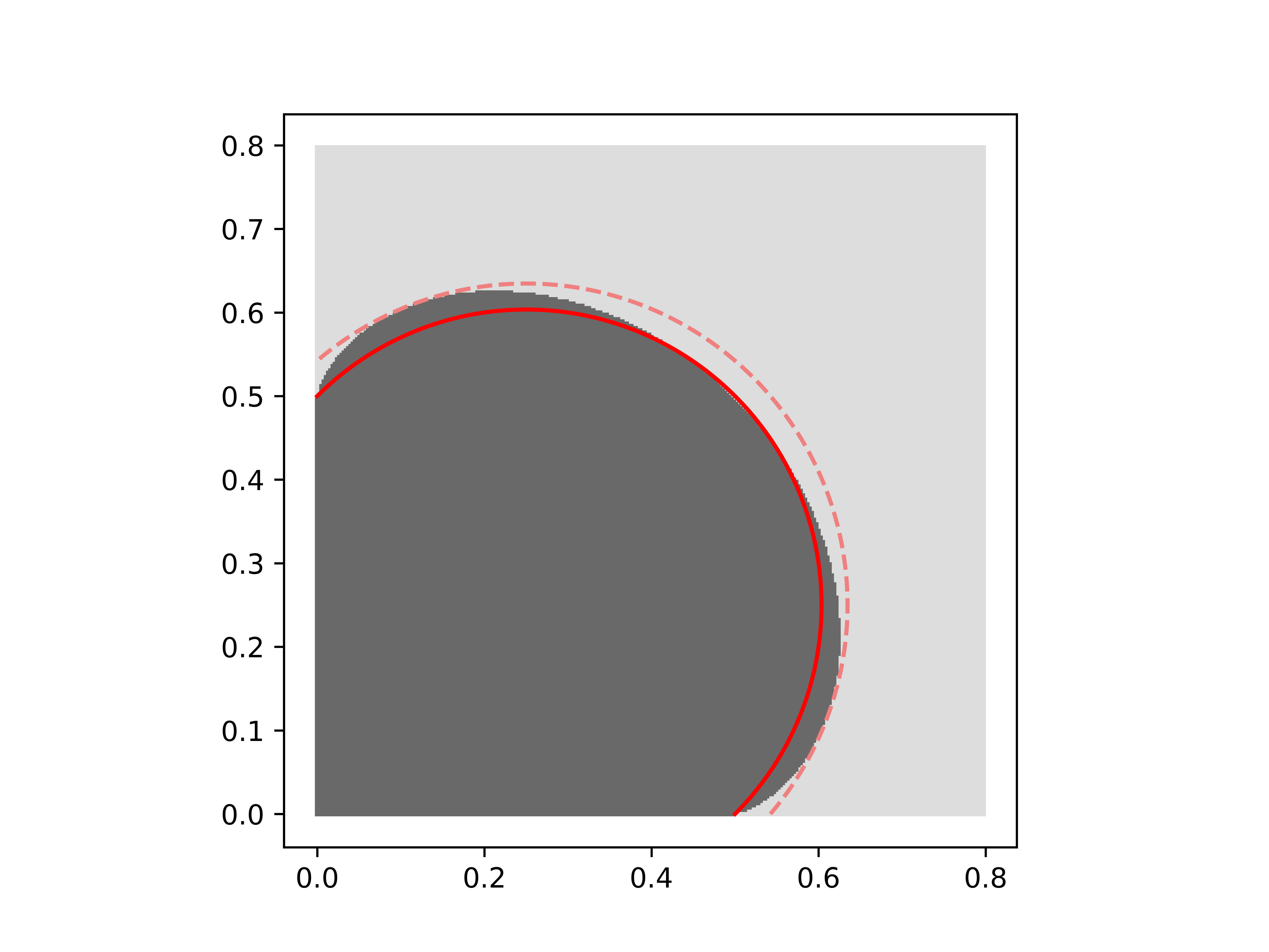
If we allow ourselves to assume that (3.9) can be extended slightly outside the parameter domain , it is natural to consider parameters for which (3.17) vanishes. This occurs precisely on the circular segment
| (5.1) |
which is illustrated in Figure 2. To be specific, we recall that defined in (3.10) provides an upper bound of and that
By replacing all occurrences of the natural number with the real variable on the right-hand side, we obtain the function from (3.15). We previously saw in (3.16) that
and that the leading term vanishes precisely when . This indicates that the convergence of as is “rapid” in this case. If , then will eventually be positive if is large enough. We therefore believe that the monotonicity properties of change somewhere in the vicinity of the circle
| (5.2) |
Replacing the variables by transfers the circular segment (5.2) precisely to (5.1).
Since we do not know how far the inequality
can be extended outside of , our theoretical approach cannot be applied to study this case. We resort to a numerical investigation of the behavior of the corresponding Widom factors using a generalization of the Remez algorithm due to Tang [42, 43, 22, 26]. See also [39] for an overview on how this algorithm can be applied to the numerical study of Chebyshev polynomials. The numerical results are illustrated in Figure 3. It is clearly suggested by these plots that in the vicinity of the set specified in (5.1), the monotonicity properties of seem to shift from monotonically increasing to monotonically decreasing as we move from the inside of the disk to its exterior. Since these considerations are based on numerical experiments, we are left to speculate if this is indeed the true picture. We formulate the following conjecture.
Conjecture 5.2.
Suppose that .
-
(1)
If
then is monotonically increasing to as .
-
(2)
If
then is monotonically decreasing to as .
6. Appendix
For the benefit of the reader we restate the definitions of the terms and as defined in (3.19) and (3.18).
We aim to show that these are upper bounded by in the parameter domain . This is a necessary part of proving Lemma 3.2.
Lemma 6.1.
If , then for with equality if and only if .
Proof.
To show that this is indeed true, we perform a detailed analysis of the coefficients on the set illustrated in Figure 4.
The boundary of is parametrized with through
Based on these factorizations it becomes apparent that and holds for but these values of are precisely those which correspond to the boundary of with the vertices removed.
Differentiating for with respect to yields
| (6.1) | ||||
| (6.2) | ||||
| (6.3) | ||||
| (6.4) |
We begin with showing that unless the parameters belong to the vertices of . Assuming that we obtain from (6.3) that
In particular, this implies that
is a convex function on for any fixed . Consequently, if then
| (6.5) |
Clearly, the quantity
is negative if . We claim that the same is true for . To see this we introduce the function which is given by
Differentiating two times we obtain
It is evident that is convex if . On the other hand, if then
which shows that is decreasing on . Consequently, if we have
By refering to (6.5) we obtain
and therefore is strictly decreasing on . From (6.2) we gather that if then for any ,
This implies that defines a convex function on and since we already concluded that is strictly decreasing on , we find that for any fixed
and if and only if . This in particular shows that with equality if and only if or and .
We now proceed to study the coefficient and show that holds on the parameter domain . This turns out to be straightforward. From (6.4) we find that
| (6.6) | |||
| (6.7) |
Since , we have
and consequently the sign of coincides with that of
This is sufficient to conclude that the maximum of on must be attained at an endpoint of and we gather that
with equality attained if and only if . ∎
Acknowledgement
This study originated from discussions held during a SQuaRE meeting at the American Institute of Mathematics (AIM) facility in Pasadena, CA. We extend our heartfelt gratitude to AIM for their generous hospitality and for creating such an inspiring scientific environment.
References
- [1] N. I. Achieser. Theory of approximation. Frederick Ungar publishing co. New York, 1956.
- [2] G. Alpan. Extremal polynomials on a Jordan arc. J. Approx. Theory, 276:105708, 2022.
- [3] G. Alpan and M. Zinchenko. On the Widom factors for extremal polynomials. J. Approx. Theory, 259:105480, 2020.
- [4] G. Alpan and M. Zinchenko. Lower bounds for weighted Chebyshev and orthogonal polynomials. arXiv, math.CA, 2408.11496, 2024.
- [5] V. A. Antonov and K .V. Holšhevnikov. Estimation of a remainder of a Legendre inequality (russian). Vestnik Leningrad Univ. Math., 13:163–166, 1981.
- [6] P. Baratella. Bounds for the error in Hilb formula for Jacobi polynomials. Atti Acc. Scienze Torino, Cl.Sci.Fis.Mat.Natur., 120:207–223.
- [7] A. Bergman and O. Rubin. Chebyshev polynomials corresponding to a vanishing weight. J. Approx. Theory, 301:106048, 2024.
- [8] S. N. Bernstein. Sur les polynômes orthogonaux relatifs à un segment fini. J. Math., 90:127–177, 1930.
- [9] S. N. Bernstein. Sur les polynômes orthogonaux relatifs à un segment fini (second partie). J. Math., 10:219–286, 1931.
- [10] P. L. Chebyshev. Théorie des mécanismes connus sous le nom de parallélogrammes. Mém. des sav. étr. prés. à l’Acad. de. St. Pétersb., 7:539–568, 1854.
- [11] P. L. Chebyshev. Ser les questions de minima qui se rattachent a la représentation approximative des fonctions. Mém. Acad. Sci. Pétersb., 7:199–291, 1859.
- [12] Y. Chow, L. Gatteschi, and R. Wong. A Bernstein-type inequality for the Jacobi polynomial. Proc. Am. Math. Soc., 121(3):703–709, 1994.
- [13] J. S. Christiansen, B. Eichinger, and O. Rubin. Extremal polynomials and sets of minimal capacity. Constr. Approx. (to appear), 2024.
- [14] J. S. Christiansen, B. Simon, and M. Zinchenko. Asymptotics of Chebyshev polynomials, I. subsets of . Invent. Math., 208:217–245, 2017.
- [15] J. S. Christiansen, B. Simon, and M. Zinchenko. Asymptotics of Chebyshev polynomials, III. sets saturating Szegő, Schiefermayr, and Totik–Widom bounds. Oper. Theory Adv. Appl., 276:231–246, 2020.
- [16] J. S. Christiansen, B. Simon, and M. Zinchenko. Asymptotics of Chebyshev polynomials, IV. comments on the complex case. JAMA, 141:207–223, 2020.
- [17] J. S. Christiansen, B. Simon, and M. Zinchenko. Widom Factors and Szegő–Widom Asymptotics, a Review, pages 301–319. Springer International Publishing, 2022.
- [18] C. J. de la Vallée-Poussin. Sur les polynômes d’approximation et la représentation approchée d’un angle. Acad. Roy. de Belg. Bulletins de la Classe des Sci., 12, 1910.
- [19] T. Erdélyi, A. P. Magnus, and P. Nevai. Generalized Jacobi weights, Christoffel functions and Jacobi polynomials. 25:602–614, 1994.
- [20] G. Faber. Über Tschebyscheffsche Polynome. J. Reine Angew. Math., 150:79–106, 1919.
- [21] L. Fejér. Über die Lage der Nullstellen von Polynomen, die aus Minimumforderungen gewisser Art entspringen. Math. Ann., 85:41–45, 1922.
- [22] B. Fischer and J. Modersitzki. An algorithm for complex linear approximation based on semi-infinite programming. Numer. Algor., 5:287–297, 1993.
- [23] W. Gautschi. How sharp is Bernstein’s inequality for Jacobi polynomials? Electron. Trans. Numer. Anal., 36:1–8, 2009.
- [24] A. Goncharov and B. Hatinoğlu. Widom factors. Potential Anal., 42:671–680, 2015.
- [25] P Yuditskii J. S. Christiansen, B. Simon and M. Zinchenko. Asymptotics of Chebyshev polynomials, II: DCT subsets of . Duke Math. J., 168(2):325 – 349, 2019.
- [26] M. Z. Komodromos, S. F. Russell, and P. T. P. Tang. Design of FIR filters with complex desired frequency response using a generalized Remez algorithm. IEEE Trans. Circuits Syst. II, 42:274–278, 1995.
- [27] T. Koornwinder, A. Kostenko, and G. Teschl. Jacobi polynomials, Bernstein-type inequalities and dispersion estimates for the discrete Laguerre operator. Adv. Math., 333:796–821, 2018.
- [28] A. Kroó. A note on strong asymptotics of weighted Chebyshev polynomials. J. Approx. Theory, 181:1–5, 2014.
- [29] A. Kroó and F. Peherstorfer. Asymptotic representation of weighted - and -minimal polynomials. Math. Proc. Camb. Philos. Soc., 144:241–254, 2008.
- [30] M. Lachance, E. B. Saff, and R. S Varga. Inequalities for polynomials with a prescribed zero. Math. Z., 168:105–116, 1979.
- [31] P. D. Lax. Proof of a conjecture of P. Erdős on the derivative of a polynomial. Bull. Amer. Math. Soc., 50:509 – 513, 1944.
- [32] L. Lorch. Inequalities for ultraspherical polynomials and the gamma function. J. Approx. Theory, 40:115–120, 1984.
- [33] G. G. Lorentz. Approximation of Functions. Chelsea publishing company, New York, 1986.
- [34] D. .S Lubinsky and E. B. Saff. Strong asymptotics for extremal polynomials associated with weights on . In E. B. Saff, editor, Approximation Theory, Tampa, pages 83–104. Springer Berlin Heidelberg, 1987.
- [35] A. A. Markov. Finding the smallest and the largest values of some function that deviates least form zero. Soobshch. Kharkov Soc. Math., 1, 1884.
- [36] J. C. Mason. Chebyshev polynomials of the second, third and fourth kinds in approximation, indefinite integration, and integral transforms. J. Comput. Appl. Math., 49:169–178, 1993.
- [37] G. Novello, K. Schiefermayr, and M. Zinchenko. Weighted Chebyshev polynomials on compact subsets of the complex plane. In From operator theory to orthogonal polynomials, combinatorics, and number theory, pages 357–370. Springer, 2021.
- [38] G. Polyá and G. Szegő. Problems and theorems in analysis I. Die Grundlehren der mathematischen Wissenschaften in Einzeldarstellungen. Berlin, Heidelberg, Springer, 1972.
- [39] Olof Rubin. Computing chebyshev polynomials using the complex remez algorithm. arXiv, math.CA, 2405.05067, 2024.
- [40] V. I. Smirnov and N. A. Lebedev. Functions of a complex variable: constructive theory. The M.I.T. press, Massachusetts Institute of Technology, Cambridge, Massachusetts, 1968.
- [41] G. Szegő. Orthogonal Polynomials. Vol 23. American Math. Soc: Colloquium publ. American Mathematical Society, 1975.
- [42] P. T. P. Tang. Chebyshev approximation on the complex plane. PhD thesis, University of California at Berkeley, 1987.
- [43] P. T. P. Tang. A fast algorithm for linear complex Chebyshev approximation. Math. Comp., 51:721–739, 1988.
- [44] H. Widom. Extremal polynomials associated with a system of curves in the complex plane. Adv. Math., 3:127–232, 1969.