UCI-TR-2024-12

TUM-HEP 1520/24

Modular flavored dark matter

Alexander Baur^a,b, Mu–Chun Chen^c,, V. Knapp–Pérez^c,,
Saúl Ramos–Sánchez^a,,

^a Instituto de Física, Universidad Nacional Autónoma de México, Cd. de México C.P. 04510, México

^b Physik Department, Technische Universität München, James-Franck-Straße 1, 85748 Garching, Germany

^c Department of Physics and Astronomy, University of California, Irvine, CA 92697-4575 USA

Discrete flavor symmetries have been an appealing approach for explaining the observed flavor structure, which is not justified in the Standard Model (SM). Typically, these models require a so-called flavon field in order to give rise to the flavor structure upon the breaking of the flavor symmetry by the vacuum expectation value (VEV) of the flavon. Generally, in order to obtain the desired vacuum alignment, a flavon potential that includes additional so-called driving fields is required. On the other hand, allowing the flavor symmetry to be modular leads to a structure where the couplings are all holomorphic functions that depend only on a complex modulus, thus greatly reducing the number of parameters in the model. We show that these elements can be combined to simultaneously explain the flavor structure and dark matter (DM) relic abundance. We present a modular model with flavon vacuum alignment that allows for realistic flavor predictions while providing a successful fermionic DM candidate.

1 Introduction

The origin of the mass hierarchies and mixings among the three generations of fermions is unexplained in the SM. One possible solution to address this so-called flavor puzzle is the introduction of traditional flavor symmetries that allow for transformations among fermions of different flavors. These symmetries are independent of moduli and are known to provide explanations for the flavor structure of both the lepton and quark sectors [1, 2, 3, 4, 5, 6, 7]. To achieve these results, models endowed with traditional flavor symmetries require the introduction of two kinds of extra SM singlet scalars: i) flavons, whose VEVs are responsible for the non-trivial flavor structure of fermions, and ii) driving fields [8, 9, 10, 11, 12, 13, 14, 15] that help to shape a suitable potential for obtaining the desired VEV pattern. The traditional flavor symmetry framework based on non-Abelian discrete symmetries has also proven helpful for DM, where the flavor symmetry plays the role of a stabilizer symmetry [16]. Furthermore, (not necessarily discrete) flavor symmetries can be successfully combined to explain both DM and flavor anomalies from SM decays [17, 18, 19].

Another promising approach to explain the flavor parameters without introducing many scalars is provided by so-called modular flavor symmetries [20, 21, 22, 23, 24, 25, 26, 27, 28, 29]. This approach has produced good fits for leptons [30, 22, 31, 32, 33, 34, 35, 25, 36, 37, 28, 38, 39, 40, 41] and quarks [24, 42, 43, 44, 45, 46, 47, 48, 49, 50, 51, 52, 53]. In this scenario, instead of depending on flavon VEVs, Yukawa couplings are replaced by multiplets of modular forms depending on the half-period ratio $\tau$, which can be considered a complex modulus. The basic problem then reduces to explaining why $\tau$ stabilizes at its best-fit value $\langle\tau\rangle$, for which being close to the symmetry-enhanced points $\tau=\mathrm{i},\;\mathrm{e}^{\nicefrac{{2\pi\mathrm{i}}}{{3}}},\;\mathrm{i}\infty$ can be advantageous [54, 55, 56, 57, 58]. Although this scheme has the potential to avoid the need for any additional scalar field, the presence of flavons in addition to the modulus can be useful too (see, e.g., Model 1 of [20] and [21]). Similarly to the traditional flavor case, modular flavor symmetries can also serve as stabilizer symmetries for DM candidates [59, 60, 61, 62, 63]

Modular flavor symmetries arise naturally in top-down constructions, such as magnetized extra dimensions [64, 65, 66, 67, 68, 69, 70, 71, 72, 73, 74, 75, 76, 77] or heterotic string orbifolds [78, 79, 80, 81, 82, 83, 84, 85, 86, 87, 88, 89], where they combine with traditional flavor symmetries, building an eclectic flavor group [90]. Remarkably, these top-down approaches provide a natural scheme where not only realistic predictions arise [88], but also the modulus $\tau$ can be stabilized close to symmetry-enhanced points [91, 92, 93, 94, 95, 96, 97].

Motivated by these observations, we propose a new supersymmetric model combined with modular flavor symmetries, which simultaneously accomplishes the following:

1. Addressing the flavor puzzle, specifically the origin of the lepton masses and mixing parameters;

2. Achieving the vacuum alignment for the flavons;

3. Providing a suitable DM candidate with the correct observed DM abundance, $\Omega_{\text{DM}}=0.265(7)$ [98].

In order to tackle these issues, we propose a simple supersymmetric model based on a $\Gamma_{3}\cong A_{4}$ modular flavor symmetry. The model resembles Model 1 of [20], where the neutrino masses arise from a Weinberg operator and the charged-lepton Yukawa couplings are given by the VEV of a flavon. It also resembles the proposal of [99], which studies a DM candidate in a non-modular $A_{4}$ model without fitting flavor parameters. In our model, the flavon potential is fixed by the flavor symmetry together with a $\mathrm{U}(1)_{\mathrm{R}}\times\mathbbm{Z}_{2}$ symmetry, which determines the couplings between the driving field and flavon superfields. The model gives a very good fit to the leptonic flavor parameters, with a low value of $\chi^{2}$. Finally, we identify a Dirac fermion composed by the Weyl fermionic parts of both the driving field and flavon superfields; we perform a parameter scan for a correct DM abundance. The goal of this model is to present a “proof of principle” that driving fields in modular supersymmetric flavor models can account for both the flavon VEV $\left\langle\phi\right\rangle$ and DM.

Our paper is organized as follows. In Section 2, we review the basics of modular symmetries and its application to solving the flavor puzzle. In Section 3, we define our model. In Section 4, we present the numerical fit for the lepton flavor parameters. In Section 5, we analyze the relevant terms for DM production. We also argue why we need freeze-in (as opposed to the more traditional freeze-out) mechanism for our model to work. We then present a parameter scan for the available parameter space for our DM candidate. Finally, in Section 6 we summarize our results and future directions for further constraints.

2 Modular symmetry

2.1 Modular groups and modular forms

The modular group $\Gamma:=\mathrm{SL}(2,\mathbbm{Z})$ is given by

$$\Gamma\leavevmode\nobreak\ =\leavevmode\nobreak\ \left\{\begin{pmatrix}a&b\\ c&d\end{pmatrix}\leavevmode\nobreak\ \Big{|}\leavevmode\nobreak\ a,b,c,d\in\mathbbm{Z}\;\&\;ad-bc=1\right\}\;,$$ (1)

and can be generated by

$$S\leavevmode\nobreak\ =\leavevmode\nobreak\ \begin{pmatrix}0&1\\ -1&0\end{pmatrix}\qquad\text{ and }\qquad T\leavevmode\nobreak\ =\leavevmode\nobreak\ \begin{pmatrix}1&1\\ 0&1\end{pmatrix}\;,$$ (2)

which satisfy the general presentation of $\Gamma$, $\langle S,T\leavevmode\nobreak\ |\leavevmode\nobreak\ S^{4}=(ST)^{3}=\mathbbm{1},S^{2}T=TS^{2}\rangle$. The principle congruence subgroups of level $N$ of $\Gamma$ are defined as

$$\Gamma(N)\leavevmode\nobreak\ :=\leavevmode\nobreak\ \left\{\gamma\in\Gamma\leavevmode\nobreak\ |\leavevmode\nobreak\ \gamma=\mathbbm{1}\mod N\right\}\,,$$ (3)

which are infinite normal subgroups of $\Gamma$ with finite index. We can also define the inhomogeneous modular group $\overline{\Gamma}:=\Gamma/\{\pm\mathbbm{1}\}\cong\mathrm{PSL}(2,\mathbbm{Z})$ and its subgroups $\overline{\Gamma}(N)$ with $\overline{\Gamma}(2):=\Gamma(2)/\{\pm\mathbbm{1}\}$ and $\overline{\Gamma}(N):=\Gamma(N)$ for $N>2$ (as $-\mathbbm{1}$ does not belong to $\Gamma(N)$). An element $\gamma$ of a modular group acts on the half-period ratio, modulus $\tau$, as

$$\gamma\,\tau\leavevmode\nobreak\ =\leavevmode\nobreak\ \frac{a\tau+b}{c\tau+d}\,,\qquad\text{where}\quad\tau\in\mathcal{H}$$ (4)

and $\mathcal{H}$ is the upper complex half-plane,

$$\mathcal{H}\leavevmode\nobreak\ :=\leavevmode\nobreak\ \{\tau\in\mathbbm{C}\;|\;\operatorname{Im}\tau>0\}\;.$$ (5)

Modular forms $f(\tau)$ of positive modular weight $k$ and level $N$ are complex functions of $\tau$, holomorphic in $\mathcal{H}$, and transform as

$$f(\tau)\leavevmode\nobreak\ \stackrel{{\scriptstyle\gamma}}{{\longrightarrow}}\leavevmode\nobreak\ f(\gamma\,\tau)\leavevmode\nobreak\ =\leavevmode\nobreak\ (c\tau+d)^{k}\,f(\tau)\,,\qquad\gamma\in\Gamma(N)\;.$$ (6)

In this work, we restrict ourselves to even modular weights, $k\in 2\mathbbm{N}$, although it is known that modular weights can be odd [28] or fractional [100, 72] in certain scenarios. Interestingly, modular forms with fixed weight $k$ and level $N$ build finite-dimensional vector spaces, which close under the action of $\Gamma$. It follows then that they must build representations of a finite modular group that, for even modular weights, result from the quotient

$$\Gamma_{N}\leavevmode\nobreak\ :=\leavevmode\nobreak\ \overline{\Gamma}/\overline{\Gamma}(N)\,.$$ (7)

Then, under a finite modular transformation $\gamma\in\Gamma$, modular forms of weight $k$ are $n$-plets (which are called vector-valued modular forms [101]) $Y(\tau):=\left(f_{1}(\tau),f_{2}(\tau),\ldots,f_{n}(\tau)\right)^{\mathrm{T}}$ of $\Gamma_{N}$, transforming as

$$Y(\tau)\leavevmode\nobreak\ \stackrel{{\scriptstyle\gamma}}{{\longrightarrow}}\leavevmode\nobreak\ Y(\gamma\,\tau)\leavevmode\nobreak\ =\leavevmode\nobreak\ (c\tau+d)^{k}\,\rho(\gamma)\,Y(\tau)\,,$$ (8)

where $\rho(\gamma)\in\Gamma_{N}$ is a representation of $\gamma$.

2.1.1 Finite modular group $\Gamma_{3}\cong A_{4}$

As our model is based on $\Gamma_{3}\cong A_{4}$, let us discuss some general features of this group and its modular forms. $\Gamma_{3}$ is defined by the presentation

$$\Gamma_{3}\leavevmode\nobreak\ =\leavevmode\nobreak\ \left\langle S,T\leavevmode\nobreak\ |\leavevmode\nobreak\ S^{2}\leavevmode\nobreak\ =\leavevmode\nobreak\ (ST)^{3}\leavevmode\nobreak\ =\leavevmode\nobreak\ T^{3}\leavevmode\nobreak\ =\leavevmode\nobreak\ \mathbbm{1}\right\rangle\,.$$ (9)

It has order 12 and the irreducible representations (in the complex basis) are given in Table 1.

	${\boldsymbol{1}}$	${\boldsymbol{1}}^{\prime}$	${\boldsymbol{1}}^{\prime\prime}$	${\boldsymbol{3}}$		${\boldsymbol{1}}$	${\boldsymbol{1}}^{\prime}$	${\boldsymbol{1}}^{\prime\prime}$	${\boldsymbol{3}}$
$\rho(S)$	$1$	$1$	$1$	$\frac{1}{3}\begin{pmatrix}-1&2&2\\ 2&-1&2\\ 2&2&-1\end{pmatrix}$	$\rho(T)$	$1$	$\omega$	$\omega^{2}$	$\begin{pmatrix}1&0&0\\ 0&\omega&0\\ 0&0&\omega^{2}\end{pmatrix}$

Table 1: Irreducible representations of $\Gamma_{3}\cong A_{4}$. Here, $\omega:=\mathrm{e}^{\nicefrac{{2\pi\mathrm{i}}}{{3}}}$.

Besides ${\boldsymbol{1}}^{a}\otimes{\boldsymbol{1}}^{b}={\boldsymbol{1}}^{c}$ with $c=a+b\mod 3$ and ${\boldsymbol{1}}^{a}\otimes{\boldsymbol{3}}={\boldsymbol{3}}$, where $a,b,c=0,1,2$ count the number of primes, we have the nontrivial product rule ${\boldsymbol{3}}\otimes{\boldsymbol{3}}={\boldsymbol{1}}\oplus{\boldsymbol{1}}^{\prime}\oplus{\boldsymbol{1}}^{\prime\prime}\oplus{\boldsymbol{3}}_{S}\oplus{\boldsymbol{3}}_{A}$, where $S$ and $A$ stand respectively for symmetric and antisymmetric. Considering two triplets $\rho=(\rho_{1},\rho_{2},\rho_{3})^{\mathrm{T}}$ and $\psi=(\psi_{1},\psi_{2},\psi_{3})^{\mathrm{T}}$, in our conventions the Clebsch-Gordan coefficients of $\rho\otimes\psi$ are

$$(\rho\otimes\psi)_{{\boldsymbol{1}}} =\rho_{1}\psi_{1}+\rho_{2}\psi_{3}+\rho_{3}\psi_{2}\,,\quad (\rho\otimes\psi)_{{\boldsymbol{1}}^{\prime}} =\rho_{1}\psi_{2}+\rho_{2}\psi_{1}+\rho_{3}\psi_{3}\,,$$ (10)

$$(\rho\otimes\psi)_{{\boldsymbol{1}}^{\prime\prime}} =\rho_{1}\psi_{3}+\rho_{2}\psi_{2}+\rho_{3}\psi_{1}\,,$$

$$(\rho\otimes\psi)_{{\boldsymbol{3}}_{S}} =\frac{1}{\sqrt{3}}\begin{pmatrix}2\rho_{1}\psi_{1}-\rho_{2}\psi_{3}-\rho_{3}\psi_{2}\\ 2\rho_{3}\psi_{3}-\rho_{1}\psi_{2}-\rho_{2}\psi_{1}\\ 2\rho_{2}\psi_{2}-\rho_{3}\psi_{1}-\rho_{1}\psi_{3}\end{pmatrix}, (\rho\otimes\psi)_{{\boldsymbol{3}}_{A}} =\begin{pmatrix}\rho_{2}\psi_{3}-\rho_{3}\psi_{2}\\ \rho_{1}\psi_{2}-\rho_{2}\psi_{1}\\ \rho_{3}\psi_{1}-\rho_{1}\psi_{3}\\ \end{pmatrix}.$$

The lowest-weight modular forms of $\Gamma_{3}$ furnish a triplet $Y=(Y_{1},Y_{2},Y_{3})^{\mathrm{T}}$ of weight $k_{Y}=2$, whose components are given by [20]

$$Y_{1}(\tau) =\leavevmode\nobreak\ \frac{\mathrm{i}}{2\pi}\left[\frac{\eta^{\prime}\left(\frac{\tau}{3}\right)}{\eta\left(\frac{\tau}{3}\right)}+\frac{\eta^{\prime}\left(\frac{\tau+1}{3}\right)}{\eta\left(\frac{\tau+1}{3}\right)}+\frac{\eta^{\prime}\left(\frac{\tau+2}{3}\right)}{\eta\left(\frac{\tau+2}{3}\right)}-\frac{27\eta^{\prime}(3\tau)}{\eta(3\tau)}\right]\,,$$ (11)

$$Y_{2}(\tau) =\leavevmode\nobreak\ -\frac{\mathrm{i}}{\pi}\left[\frac{\eta^{\prime}\left(\frac{\tau}{3}\right)}{\eta\left(\frac{\tau}{3}\right)}+\omega^{2}\frac{\eta^{\prime}\left(\frac{\tau+1}{3}\right)}{\eta\left(\frac{\tau+1}{3}\right)}+\omega\frac{\eta^{\prime}\left(\frac{\tau+2}{3}\right)}{\eta\left(\frac{\tau+2}{3}\right)}\right]\,,$$

$$Y_{3}(\tau) =\leavevmode\nobreak\ -\frac{\mathrm{i}}{\pi}\left[\frac{\eta^{\prime}\left(\frac{\tau}{3}\right)}{\eta\left(\frac{\tau}{3}\right)}+\omega\frac{\eta^{\prime}\left(\frac{\tau+1}{3}\right)}{\eta\left(\frac{\tau+1}{3}\right)}+\omega^{2}\frac{\eta^{\prime}\left(\frac{\tau+2}{3}\right)}{\eta\left(\frac{\tau+2}{3}\right)}\right]\,,$$

where $\eta(\tau)$ is the so-called Dedekind $\eta$ function

$$\eta(\tau)\leavevmode\nobreak\ =\leavevmode\nobreak\ q^{\nicefrac{{1}}{{24}}}\prod_{n=1}^{\infty}(1-q^{n})\qquad\text{with}\qquad q:=\mathrm{e}^{2\pi\mathrm{i}\tau}\;.$$ (12)

Higher-weight modular forms can be constructed from the tensor products of the weight $2$ modular forms given in Equation 11.

2.2 Modular supersymmetric theories

We consider models with $\mathcal{N}=1$ global supersymmetry (SUSY), defined by the Lagrange density

$$\mathcal{L}\leavevmode\nobreak\ =\leavevmode\nobreak\ \int\mathrm{d}^{2}\theta\,\mathrm{d}^{2}\bar{\theta}\,K(\Phi,\overline{\Phi})+\left(\int\mathrm{d}^{2}\,\theta\,W(\Phi)+\text{h.c.}\right)\,,$$ (13)

where $K(\Phi,\overline{\Phi})$ is the Kähler potential, $W(\Phi)$ is the superpotential, and $\Phi$ denotes collectively all matter superfields $\varphi^{i}$ of the theory and the modulus $\tau$.

Under an element of the modular symmetry $\gamma\in\Gamma$, $\tau$ transforms according to Equation 4, and matter superfields are assumed to transform as

$$\varphi^{i}\leavevmode\nobreak\ \lx@xy@svg{\hbox{\raise 0.0pt\hbox{\kern 3.0pt\hbox{\ignorespaces\ignorespaces\ignorespaces\hbox{\vtop{\kern 0.0pt\offinterlineskip\halign{\entry@#!@&&\entry@@#!@\cr&\crcr}}}\ignorespaces{\hbox{\kern-3.0pt\raise 0.0pt\hbox{\hbox{\kern 0.0pt\raise 0.0pt\hbox{\hbox{\kern 3.0pt\raise 0.0pt\hbox{$\textstyle{{}\ignorespaces\ignorespaces\ignorespaces\ignorespaces}$}}}}}}}\ignorespaces\ignorespaces\ignorespaces\ignorespaces{}{\hbox{\lx@xy@droprule}}\ignorespaces\ignorespaces\ignorespaces{\hbox{\kern 5.0pt\raise 5.1875pt\hbox{{}\hbox{\kern 0.0pt\raise 0.0pt\hbox{\hbox{\kern 3.0pt\hbox{\hbox{\kern 0.0pt\raise-0.8264pt\hbox{$\scriptstyle{\gamma}$}}}\kern 3.0pt}}}}}}\ignorespaces\ignorespaces{\hbox{\kern 6.81206pt\raise 0.0pt\hbox{{}\hbox{\kern 0.0pt\raise 0.0pt\hbox{\hbox{\kern 3.0pt\hbox{\hbox{\kern 0.0pt\raise 0.0pt\hbox{$\scriptstyle{}$}}}\kern 3.0pt}}}}}}\ignorespaces{\hbox{\kern 16.62413pt\raise 0.0pt\hbox{\hbox{\kern 0.0pt\raise 0.0pt\hbox{\lx@xy@tip{1}\lx@xy@tip{-1}}}}}}{\hbox{\lx@xy@droprule}}{\hbox{\lx@xy@droprule}}{\hbox{\kern 16.62413pt\raise 0.0pt\hbox{\hbox{\kern 0.0pt\raise 0.0pt\hbox{\hbox{\kern 3.0pt\raise 0.0pt\hbox{$\textstyle{}$}}}}}}}\ignorespaces}}}}\ignorespaces\leavevmode\nobreak\ (c\tau+d)^{-k_{i}}\rho_{i}(\gamma)\,\varphi^{i}\,, \scriptstyle{\gamma} \scriptstyle{\gamma}$$ (14)

where $k_{i}$ are also called modular weights of the field $\varphi^{i}$, which transform as $\Gamma_{N}$ multiplets. Modular weights $k_{i}$ are not restricted to be positive integers because $\varphi^{i}$ are not modular forms. Analogous to Equation 8, the matrix $\rho_{i}(\gamma)$ is a representation of the finite modular flavor group $\Gamma_{N}$.

For simplicity, we assume a minimal Kähler potential of the form

$$K(\Phi,\overline{\Phi})\leavevmode\nobreak\ =\leavevmode\nobreak\ -\log(-\mathrm{i}\tau+\mathrm{i}\bar{\tau})+\sum_{i}(-\mathrm{i}\tau+\mathrm{i}\bar{\tau})^{-k_{i}}|\varphi^{i}|^{2}\,.$$ (15)

Making use of Equation 14, we see that $K(\Phi,\overline{\Phi})$ transforms under a modular transformation $\gamma\in\Gamma$ as

$$K(\Phi,\overline{\Phi})\leavevmode\nobreak\ \lx@xy@svg{\hbox{\raise 0.0pt\hbox{\kern 3.0pt\hbox{\ignorespaces\ignorespaces\ignorespaces\hbox{\vtop{\kern 0.0pt\offinterlineskip\halign{\entry@#!@&&\entry@@#!@\cr&\crcr}}}\ignorespaces{\hbox{\kern-3.0pt\raise 0.0pt\hbox{\hbox{\kern 0.0pt\raise 0.0pt\hbox{\hbox{\kern 3.0pt\raise 0.0pt\hbox{$\textstyle{{}\ignorespaces\ignorespaces\ignorespaces\ignorespaces}$}}}}}}}\ignorespaces\ignorespaces\ignorespaces\ignorespaces{}{\hbox{\lx@xy@droprule}}\ignorespaces\ignorespaces\ignorespaces{\hbox{\kern 5.0pt\raise 5.1875pt\hbox{{}\hbox{\kern 0.0pt\raise 0.0pt\hbox{\hbox{\kern 3.0pt\hbox{\hbox{\kern 0.0pt\raise-0.8264pt\hbox{$\scriptstyle{\gamma}$}}}\kern 3.0pt}}}}}}\ignorespaces\ignorespaces{\hbox{\kern 6.81206pt\raise 0.0pt\hbox{{}\hbox{\kern 0.0pt\raise 0.0pt\hbox{\hbox{\kern 3.0pt\hbox{\hbox{\kern 0.0pt\raise 0.0pt\hbox{$\scriptstyle{}$}}}\kern 3.0pt}}}}}}\ignorespaces{\hbox{\kern 16.62413pt\raise 0.0pt\hbox{\hbox{\kern 0.0pt\raise 0.0pt\hbox{\lx@xy@tip{1}\lx@xy@tip{-1}}}}}}{\hbox{\lx@xy@droprule}}{\hbox{\lx@xy@droprule}}{\hbox{\kern 16.62413pt\raise 0.0pt\hbox{\hbox{\kern 0.0pt\raise 0.0pt\hbox{\hbox{\kern 3.0pt\raise 0.0pt\hbox{$\textstyle{}$}}}}}}}\ignorespaces}}}}\ignorespaces\leavevmode\nobreak\ K(\Phi,\overline{\Phi})+\log(c\tau+d)+\log(c\bar{\tau}+d)\,. \scriptstyle{\gamma} \scriptstyle{\gamma}$$ (16)

Thus, realizing that the Kähler potential is left invariant up to a global supersymmetric Kähler transformation, in order for the Lagrange density of Equation 13 to be modular invariant, we need the superpotential to be invariant under modular transformations, i.e.

$$W(\Phi)\leavevmode\nobreak\ \lx@xy@svg{\hbox{\raise 0.0pt\hbox{\kern 3.0pt\hbox{\ignorespaces\ignorespaces\ignorespaces\hbox{\vtop{\kern 0.0pt\offinterlineskip\halign{\entry@#!@&&\entry@@#!@\cr&\crcr}}}\ignorespaces{\hbox{\kern-3.0pt\raise 0.0pt\hbox{\hbox{\kern 0.0pt\raise 0.0pt\hbox{\hbox{\kern 3.0pt\raise 0.0pt\hbox{$\textstyle{{}\ignorespaces\ignorespaces\ignorespaces\ignorespaces}$}}}}}}}\ignorespaces\ignorespaces\ignorespaces\ignorespaces{}{\hbox{\lx@xy@droprule}}\ignorespaces\ignorespaces\ignorespaces{\hbox{\kern 5.0pt\raise 5.1875pt\hbox{{}\hbox{\kern 0.0pt\raise 0.0pt\hbox{\hbox{\kern 3.0pt\hbox{\hbox{\kern 0.0pt\raise-0.8264pt\hbox{$\scriptstyle{\gamma}$}}}\kern 3.0pt}}}}}}\ignorespaces\ignorespaces{\hbox{\kern 6.81206pt\raise 0.0pt\hbox{{}\hbox{\kern 0.0pt\raise 0.0pt\hbox{\hbox{\kern 3.0pt\hbox{\hbox{\kern 0.0pt\raise 0.0pt\hbox{$\scriptstyle{}$}}}\kern 3.0pt}}}}}}\ignorespaces{\hbox{\kern 16.62413pt\raise 0.0pt\hbox{\hbox{\kern 0.0pt\raise 0.0pt\hbox{\lx@xy@tip{1}\lx@xy@tip{-1}}}}}}{\hbox{\lx@xy@droprule}}{\hbox{\lx@xy@droprule}}{\hbox{\kern 16.62413pt\raise 0.0pt\hbox{\hbox{\kern 0.0pt\raise 0.0pt\hbox{\hbox{\kern 3.0pt\raise 0.0pt\hbox{$\textstyle{}$}}}}}}}\ignorespaces}}}}\ignorespaces\leavevmode\nobreak\ W(\Phi)\,. \scriptstyle{\gamma} \scriptstyle{\gamma}$$ (17)

The superpotential $W(\Phi)$ has the general form

$$W(\Phi)\leavevmode\nobreak\ =\leavevmode\nobreak\ \mu_{ij}(\tau)\varphi^{i}\varphi^{j}+Y_{ijk}(\tau)\varphi^{i}\varphi^{j}\varphi^{k}+G_{ijk\ell}(\tau)\varphi^{i}\varphi^{j}\varphi^{k}\varphi^{\ell}\;,$$ (18)

where $\mu_{ij}(\tau)$, $Y_{ijk}(\tau)$ and $G_{ijk}(\tau)$ are modular forms of level $N$. Because of Equation 17, each term of Equation 18 must be modular invariant. Let us illustrate how we can achieve this by taking the trilinear coupling $Y_{ijk}(\tau)\varphi^{i}\varphi^{j}\varphi^{k}$. The Yukawa coupling $Y_{ijk}$ transforms under a modular transformation $\gamma\in\Gamma$ as

$$Y_{ijk}(\tau)\leavevmode\nobreak\ \lx@xy@svg{\hbox{\raise 0.0pt\hbox{\kern 3.0pt\hbox{\ignorespaces\ignorespaces\ignorespaces\hbox{\vtop{\kern 0.0pt\offinterlineskip\halign{\entry@#!@&&\entry@@#!@\cr&\crcr}}}\ignorespaces{\hbox{\kern-3.0pt\raise 0.0pt\hbox{\hbox{\kern 0.0pt\raise 0.0pt\hbox{\hbox{\kern 3.0pt\raise 0.0pt\hbox{$\textstyle{{}\ignorespaces\ignorespaces\ignorespaces\ignorespaces}$}}}}}}}\ignorespaces\ignorespaces\ignorespaces\ignorespaces{}{\hbox{\lx@xy@droprule}}\ignorespaces\ignorespaces\ignorespaces{\hbox{\kern 5.0pt\raise 5.1875pt\hbox{{}\hbox{\kern 0.0pt\raise 0.0pt\hbox{\hbox{\kern 3.0pt\hbox{\hbox{\kern 0.0pt\raise-0.8264pt\hbox{$\scriptstyle{\gamma}$}}}\kern 3.0pt}}}}}}\ignorespaces\ignorespaces{\hbox{\kern 6.81206pt\raise 0.0pt\hbox{{}\hbox{\kern 0.0pt\raise 0.0pt\hbox{\hbox{\kern 3.0pt\hbox{\hbox{\kern 0.0pt\raise 0.0pt\hbox{$\scriptstyle{}$}}}\kern 3.0pt}}}}}}\ignorespaces{\hbox{\kern 16.62413pt\raise 0.0pt\hbox{\hbox{\kern 0.0pt\raise 0.0pt\hbox{\lx@xy@tip{1}\lx@xy@tip{-1}}}}}}{\hbox{\lx@xy@droprule}}{\hbox{\lx@xy@droprule}}{\hbox{\kern 16.62413pt\raise 0.0pt\hbox{\hbox{\kern 0.0pt\raise 0.0pt\hbox{\hbox{\kern 3.0pt\raise 0.0pt\hbox{$\textstyle{}$}}}}}}}\ignorespaces}}}}\ignorespaces\leavevmode\nobreak\ (c\tau+d)^{k_{Y}}\rho_{Y}(\gamma)\,Y_{ijk}(\tau)\,, \scriptstyle{\gamma} \scriptstyle{\gamma}$$ (19)

where $k_{Y}$ is the even integer modular weight of the modular form $Y_{ijk}(\tau)$. Then, for $Y_{ijk}(\tau)\varphi^{i}\varphi^{j}\varphi^{k}$ to be invariant and using the superfield transformations of Equation 14, we must demand that $k_{Y}=k_{i}+k_{j}+k_{k}$ and that the product $\rho_{Y}\otimes\rho_{i}\otimes\rho_{j}\otimes\rho_{k}$ contains an invariant singlet.

Since we shall be concerned with SUSY breaking, let us briefly discuss the soft-SUSY breaking terms in the Lagrange density. They are given by

$$\mathcal{L}_{\text{soft}}\leavevmode\nobreak\ =\leavevmode\nobreak\ -\frac{1}{2}\left(M_{a}\hat{\lambda}^{a}\hat{\lambda}^{a}+\text{h.c}\right)-\tilde{m}_{i}^{2}\bar{\hat{\varphi}}^{i}\hat{\varphi}^{i}-\left(A_{ijk}\hat{\varphi}^{i}\hat{\varphi}^{j}\hat{\varphi}^{k}+B_{ij}\hat{\varphi}^{i}\hat{\varphi}^{j}+\text{h.c.}\right)\;,$$ (20)

where $M_{a}$ are the gaugino masses, $\hat{\lambda}^{a}$ are the canonically normalized gaugino fields, and $\tilde{m}_{i}$ are the soft-masses. We use a notation, where $\hat{\varphi}^{i}$ stands for both the canonically normalized chiral superfield and its scalar component [103]. We do not assume any specific source of SUSY breaking, and thus the parameters in Equation 20 are free, in principle. However, in our model $B-$terms are forbidden at tree level and the $A$-terms do not play a role in DM production at tree-level, see Section 5.

3 Dark modular flavon model

We propose a model of leptons, governed by the modular flavor group $\Gamma_{3}\cong A_{4}$. In our model, the lepton doublets $L$ transform as a flavor triplet and charged-lepton singlets $E^{\mathrm{c}}_{i}$ transform as three distinct singlets under $\Gamma_{3}$. The particle content of our model is summarized in Table 2.

	$L$	$(E_{1}^{\mathrm{c}},E_{2}^{\mathrm{c}},E_{3}^{\mathrm{c}})$	$H_{d}$	$H_{u}$	$\phi_{3}$	$\phi_{1^{\prime}}$	$\zeta_{3}$	$\zeta_{1^{\prime\prime}}$	$Y(\tau)$
$\mathrm{SU}(2)_{L}$	${\boldsymbol{2}}$	${\boldsymbol{1}}$	${\boldsymbol{2}}$	${\boldsymbol{2}}$	${\boldsymbol{1}}$	${\boldsymbol{1}}$	${\boldsymbol{1}}$	${\boldsymbol{1}}$	${\boldsymbol{1}}$
$\mathrm{U}(1)_{Y}$	$-\frac{1}{2}$	$1$	$-\frac{1}{2}$	$\frac{1}{2}$	$0$	$0$	$0$	$0$	$0$
$\Gamma_{3}\cong A_{4}$	${\boldsymbol{3}}$	$({\boldsymbol{1}},{\boldsymbol{1}}^{\prime\prime},{\boldsymbol{1}}^{\prime})$	${\boldsymbol{1}}$	${\boldsymbol{1}}$	${\boldsymbol{3}}$	${\boldsymbol{1}}^{\prime}$	${\boldsymbol{3}}$	${\boldsymbol{1}}^{\prime\prime}$	${\boldsymbol{3}}$
$k_{i}$	$1$	$0$	$-1$	$0$	$0$	$0$	$0$	$0$	$2$
$\mathrm{U}(1)_{\mathrm{R}}$	$1$	$1$	$0$	$0$	$0$	$0$	$2$	$2$	$0$
$\mathbbm{Z}_{2}$	$0$	$0$	$0$	$0$	$0$	$-1$	$0$	$-1$	$0$

Table 2: Quantum numbers under the SM gauge groups, $\mathrm{U}(1)_{\mathrm{R}}$, $\mathbbm{Z}_{2}$ and $\Gamma_{3}$, as well as modular weights $k_{i}$ of the matter fields in our model. All fields are neutral under $\mathrm{SU}(3)_{\mathrm{color}}$.

In our model, neutrino masses arise from the Weinberg operator

$$W_{\nu}\leavevmode\nobreak\ =\leavevmode\nobreak\ \frac{1}{\Lambda}\left(H_{u}LH_{u}LY(\tau)\right)_{{\boldsymbol{1}}}\;,$$ (21)

where $\Lambda$ is the neutrino-mass scale and $Y(\tau)$ is the modular-form triplet $Y=(Y_{1},Y_{2},Y_{3})^{\mathrm{T}}$ of weight $2$ given by Equation 11. Note that there exists no other modular multiplet of weight $2$ in $\Gamma_{3}\cong A_{4}$. Hence, under our assumptions, the neutrino sector obtained from Equation 21 is highly predictive as it only depends on the parameter $\tau$, the VEV $v_{u}$ of $H_{u}$, and $\Lambda$.

The charged-lepton superpotential at leading order is

$$W_{\mathrm{CL}}\leavevmode\nobreak\ =\leavevmode\nobreak\ \frac{\alpha_{1}}{\Lambda_{\phi}}E_{1}^{\mathrm{c}}H_{d}(L\phi_{3})_{{\boldsymbol{1}}}+\frac{\alpha_{2}}{\Lambda_{\phi}}E_{2}^{\mathrm{c}}H_{d}(L\phi_{3})_{{\boldsymbol{1}}^{\prime}}+\frac{\alpha_{3}}{\Lambda_{\phi}}E_{3}^{\mathrm{c}}H_{d}(L\phi_{3})_{{\boldsymbol{1}}^{\prime\prime}}\;,$$ (22)

where $\alpha_{i}$, $i=1,2,3$, are dimensionless parameters, $\Lambda_{\phi}$ denotes the flavor breaking scale, and the subindices refer to the respective $\Gamma_{3}$ singlet components of tensored matter states in the parentheses. The charged-lepton mass matrix can be determined by the $\Gamma_{3}$ triplet flavon VEV $\left\langle\phi_{3}\right\rangle$ as in Model 1 of [20]. However, we have taken a different value of $\left\langle\phi_{3}\right\rangle$, which eventually leads to a better fit.

The flavon superpotential is given by

$$W_{\phi} =\Lambda_{\phi}\beta_{1}\zeta_{3}\phi_{3}+\beta_{2}\zeta_{3}\phi_{3}\phi_{3}\;+\frac{\beta_{3}}{\Lambda_{\phi}}\zeta_{3}\phi_{3}\phi_{3}\phi_{3}+\Lambda_{\phi}\beta_{4}\zeta_{1^{\prime\prime}}\phi_{1^{\prime}}+\frac{\beta_{5}}{\Lambda_{\phi}}\zeta_{1^{\prime\prime}}\phi_{1^{\prime}}\phi_{3}\phi_{3}$$

$$+\frac{\beta_{6}}{\Lambda_{\phi}}\zeta_{3}\phi_{3}\phi_{1^{\prime}}\phi_{1^{\prime}}\;,$$ (23)

where $\beta_{i}$, $i=1,\ldots,6$, are dimensionless couplings. This superpotential gives rise to the desired VEV pattern with driving superfields $\zeta_{r}$, $r=1^{\prime\prime},3$, and an extra flavon $\phi_{1^{\prime}}$, where the subindices label the respective $A_{4}$ representations. To fix the flavon superpotential, we impose a symmetry $\mathrm{U}(1)_{\mathrm{R}}\times\mathbbm{Z}_{2}$, similarly to [8, 99]. As usual, the $\mathrm{U}(1)_{\mathrm{R}}$ $R$-symmetry forbids the renormalizable terms in the superpotential that violate lepton and/or baryon numbers. We remark that the flavon superpotential Equation 23 is important for both finding the correct vacuum alignment for the flavons, as discussed below, and for identifying a viable DM candidate as described in Section 5.

The flavon VEV is then attained by demanding that SUSY remains unbroken at a first stage, i.e. we require vanishing $F$-terms. Recall that the $F$-term scalar potential in a global supersymmetric theory is given schematically by

$$V\leavevmode\nobreak\ =\leavevmode\nobreak\ F^{i}K_{i\bar{\jmath}}\bar{F}^{\bar{\jmath}}\;,$$ (24)

where

$$F^{i}=-\frac{\partial W}{\partial\Phi^{i}}\,,\qquad\bar{F}^{\bar{\jmath}}=F^{j*}\qquad\text{and}\qquad K^{i\bar{\jmath}}=\left(K_{i\bar{\jmath}}\right)^{-1}=(-\mathrm{i}\tau+\mathrm{i}\tau)^{k_{i}}\delta_{i\bar{j}}\;.$$ (25)

Recall that a superfield $\Phi$ can be expanded in its components as [104, Equation 2.117]

$$\Phi =\Phi(x)-\mathrm{i}\theta\sigma^{\mu}\bar{\theta}\partial_{\mu}\Phi(x)-\frac{1}{4}\theta^{2}\bar{\theta}^{2}\partial^{2}\Phi(x)+\sqrt{2}\theta\psi_{\Phi}(x)$$

$$+\frac{\mathrm{i}}{\sqrt{2}}\theta^{2}\partial_{\mu}\psi_{\Phi}(x)\sigma^{\mu}\bar{\theta}+\theta^{2}F_{\Phi}(x)\;,$$ (26)

where we have used the notation that $\Phi$ represents both the superfield and its scalar component, $\psi_{\Phi}$ is the fermionic component and $F_{\Phi}$ is the $F$-term. For SUSY to be preserved, we must have $\left\langle F_{\Phi}\right\rangle=0$. We assume that the only possible sources of SUSY breaking are given either by $\tau$ or a hidden sector. Thus, we demand $\left\langle F_{\varphi^{i}}\right\rangle=0$, for all $i$, where $\varphi^{i}$ represents the matter fields in our model (cf. Equation 13). We solve these $F$-term equations at the VEV’s of the flavons $\phi_{3}$ and $\phi_{1^{\prime}}$ and Higgs fields,

$$\left\langle\phi_{3}\right\rangle=:v_{3}\left(1,a,b\right)^{T},\qquad\left\langle\phi_{1^{\prime}}\right\rangle=:v_{1^{\prime}}\;,\qquad\left\langle H_{u}\right\rangle=:v_{u}\qquad\text{and}\qquad\left\langle H_{d}\right\rangle=:v_{d}\;.$$ (27)

where we assume $a,b,v_{3},v_{1^{\prime}}\in\mathbbm{R}$. All $F$-term equations are trivially satisfied except the ones corresponding to the driving fields given by

$$\langle F_{\zeta_{3i}}\rangle\leavevmode\nobreak\ =\leavevmode\nobreak\ 0\qquad\text{and}\qquad\langle F_{\zeta_{1^{\prime\prime}}}\rangle\leavevmode\nobreak\ =\leavevmode\nobreak\ 0\;,$$ (28)

where $\zeta_{3i}$, $i=1,2,3$, are the three components of the triplet. Thus, we obtain the following relations

$$\beta_{2} \leavevmode\nobreak\ =\leavevmode\nobreak\ c_{2}(a,b)\beta_{1}\frac{\Lambda_{\phi}}{v_{3}}\,,\qquad \beta_{3} \leavevmode\nobreak\ =\leavevmode\nobreak\ c_{3}(a,b)\beta_{1}\frac{\Lambda_{\phi}^{2}}{v_{3}^{2}}\;,$$ (29)

$$\beta_{5} \leavevmode\nobreak\ =\leavevmode\nobreak\ c_{5}(a,b)\beta_{4}\frac{\Lambda_{\phi}^{2}}{v_{3}^{2}}\,, \beta_{6} \leavevmode\nobreak\ =\leavevmode\nobreak\ c_{6}(a,b)\beta_{1}\frac{\Lambda_{\phi}^{2}}{v_{1^{\prime}}^{2}}\;,$$

where $c_{i}(a,b)$, for $i=2,3,5,6$, are coefficients that depend only on the values of $a,b$. The numerical values of $a,b$ dictate the charged lepton mass matrix. Hence, they are determined by the fit to the flavor parameters that we do in Section 4. Through the flavor parameter fit, we have found values of $\left\langle\phi_{3}\right\rangle,\left\langle\phi_{1^{\prime}}\right\rangle$ that satisfy simultaneously Equation 29, thus yielding vacuum alignment.

Finally, we assume that the flavon VEV scale from Equation 27 is below $\Lambda_{\phi}$, such that

$$v_{3}\leavevmode\nobreak\ =\leavevmode\nobreak\ v_{1^{\prime}}\leavevmode\nobreak\ =\leavevmode\nobreak\ 0.1\Lambda_{\phi}\;.$$ (30)

Furthermore, we identify the DM candidate as a Dirac fermion built as a combination of the Weyl components of $\zeta_{i}$ and $\phi_{i}$ with the scalar component of the flavon $\phi_{i}$ serving as a mediator. The parameters in Equation 30 shall play an important role in finding the current DM abundance since they set the couplings in Equation 23.

4 Flavor fit

Having defined our model of modular flavored dark matter, we next assess its capability to reproduce the experimentally observed charged-lepton masses, neutrino squared mass differences, and the mixing parameters of the PMNS matrix while providing predictions for yet undetermined observables, such as the three absolute neutrino masses, the Dirac $\mathcal{CP}$ phase, and the two Majorana phases.

The explicit neutrino mass matrix can be determined from Equation 21. By calculating the tensor products to obtain the symmetry invariant part, we find that the neutrino mass matrix is predicted to be

$$M_{\nu}\leavevmode\nobreak\ =\leavevmode\nobreak\ \frac{v_{u}^{2}}{\Lambda}\begin{pmatrix}2Y_{1}&-Y_{3}&-Y_{2}\\ -Y_{3}&2Y_{2}&-Y_{1}\\ -Y_{2}&-Y_{1}&2Y_{3}\end{pmatrix}.$$ (31)

The charged-lepton mass matrix $M_{\text{CL}}$ arises from Equation 22. Substituting the flavon VEVs as defined in Equation 27 and calculating the tensor products, we arrive at

$$M_{\text{CL}}\leavevmode\nobreak\ =\leavevmode\nobreak\ \frac{v_{d}v_{3}}{\Lambda_{\phi}}\begin{pmatrix}\alpha_{1}&\alpha_{1}b&\alpha_{1}a\\ \alpha_{2}a&\alpha_{2}&\alpha_{2}b\\ \alpha_{3}b&\alpha_{3}a&\alpha_{3}\end{pmatrix}\leavevmode\nobreak\ =\leavevmode\nobreak\ 0.1v_{d}\begin{pmatrix}\alpha_{1}&\alpha_{1}b&\alpha_{1}a\\ \alpha_{2}a&\alpha_{2}&\alpha_{2}b\\ \alpha_{3}b&\alpha_{3}a&\alpha_{3}\end{pmatrix}\;,$$ (32)

where we have used Equation 30. The values of $v_{u}$ and $v_{d}$ are determined by the Higgs VEV, $v=\sqrt{v_{u}^{2}+v_{d}^{2}}=246$ GeV, and $\tan\beta=\frac{v_{u}}{v_{d}}$, which we assume to be $\tan\beta=60$. The neutrino mass scale is determined by $\Lambda$, while we choose $\alpha_{3}$ to set the mass scale of charged leptons. By using the standard procedure (see e.g. ref. [105]), one arrives at the lepton masses and the PMNS mixing matrix. For our model, the resulting 12 flavor observables depend on 6 real dimensionless parameters $\operatorname{Re}\tau$, $\operatorname{Im}\tau$, $a$, $b$, $\alpha_{1}/\alpha_{3}$, and $\alpha_{2}/\alpha_{3}$, as well as two dimensionful overall mass scales $v_{u}^{2}/\Lambda$ and $0.1v_{d}\alpha_{3}$.

observables	best-fit values
$m_{\mathrm{e}}/m_{\mu}$	$\phantom{-}0.00473\pm 0.00004$
$m_{\mu}/m_{\tau}$	$\phantom{-}0.0450\pm 0.0007$
$y_{\tau}$	$\phantom{-}0.795\pm 0.012$
$\Delta m_{21}^{2}/10^{-5}\leavevmode\nobreak\ [\mathrm{eV}^{2}]$	$\phantom{-}7.41^{+0.21}_{-0.20}$
$\Delta m_{32}^{2}/10^{-3}\leavevmode\nobreak\ [\mathrm{eV}^{2}]$	$-2.487^{+0.027}_{-0.024}$
$\sin^{2}\theta_{12}$	$\phantom{-}0.307^{+0.012}_{-0.011}$
$\sin^{2}\theta_{13}$	$\phantom{-}0.02222^{+0.00069}_{-0.00057}$
$\sin^{2}\theta_{23}$	$\phantom{-}0.568^{+0.016}_{-0.021}$
$\delta_{\mathcal{CP}}^{\ell}/\pi$	$\phantom{-}1.52^{+0.13}_{-0.15}$

Table 3: Experimental central values and $1\sigma$ uncertainties for the masses and mixing parameters of the lepton sector. The data for the neutrino oscillation parameters is taken from the global analysis NuFIT v5.3 [106] for inverted ordering taking the Super-Kamiokande data into account. The charged-lepton mass ratios and the tau Yukawa coupling $y_{\tau}$ are taken from ref. [107] with $M_{\mathrm{SUSY}}=10\,\mathrm{TeV}$, $\tan\beta=60$, and $\bar{\eta}_{b}=0$.

To show that the model can accommodate the observed flavor structure of the SM lepton sector, we scan its parameter space and compare the resulting flavor observables to experimental data, with the best-fit values shown in Table 3. As an approximate measurement of the goodness of our fit, we introduce a $\chi^{2}$ function

$$\chi^{2}\leavevmode\nobreak\ =\leavevmode\nobreak\ \sum_{i}\chi_{i}^{2}\,,$$ (33)

consisting of a quadratic sum of one-dimensional chi-square projections for each observable. Here, we assume that the uncertainties of the fitted observables are independent of each other and do not account for the small correlations among experimental errors of $\sin^{2}\theta_{23}$ and other quantities. For the mixing angles and the neutrino squared mass differences, we determine the value of $\chi_{i}^{2}$ directly from the one-dimensional projections determined by the global analysis NuFIT v5.3 [106], which are available on their website. This is necessary to account for the strong non-Gaussianities in the uncertainties of the mixing parameters in the PMNS matrix. For these observables, we refrain from considering corrections from renormalization group running, given that their contribution is expected to be small compared to the size of the experimental errors. For the charged-lepton masses, we determine the value of $\chi_{i}^{2}$ by

$$\chi_{i}\leavevmode\nobreak\ =\leavevmode\nobreak\ \dfrac{\mu_{i,\mathrm{exp.}}-\mu_{i,\mathrm{model}}}{\sigma_{i}}\;,$$ (34)

where $\mu_{i,\mathrm{model}}$ denotes the resulting value for the $i$th observable of the model, while $\mu_{i,\mathrm{exp.}}$ and $\sigma_{i}$ refer to its experimentally observed central value and the size of the $1\sigma$ uncertainty interval given in Table 3, respectively. The total value of $\chi^{2}$ for all considered observables may then be interpreted to indicate an agreement with the experimental data at a $\sqrt{\chi^{2}}\,\sigma$ confidence level (C.L.).

To scan the parameter space of the model and minimize the $\chi^{2}$ function, we use the dedicated code FlavorPy [108]. We find that the model is in agreement with current experimental observations. The best-fit point in the parameter space of our model is at

$$\tau =-0.0119+1.005\mathrm{i}\;, a =-0.392\;, b =0.380\;, 0.1\alpha_{3}v_{d} =0.130\,\mathrm{GeV}$$ (35)

$$\frac{\alpha_{1}}{\alpha_{3}} =-22.0\;, \frac{\alpha_{2}}{\alpha_{3}} =4.78\times 10^{-3}\;, \frac{v_{u}^{2}}{\Lambda} =0.0221\,\mathrm{eV}\;,$$

where we obtain $\chi^{2}=0.08$, meaning that all resulting observables are within their experimental $1\sigma$ interval, cf. also Equation 37. In Figure 1, we present the regions in moduli space that yield results with $\chi^{2}\leq 25$.

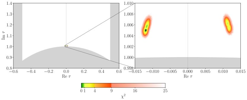
Figure 1: Regions in moduli space that yield fits with $\chi^{2}\leq 25$. The green, yellow, and orange colored regions may be interpreted as the $1\sigma$, $2\sigma$, and $3\sigma$ confidence intervals, respectively, while the opaque red fades out until the $5\sigma$ barrier is reached. The best-fit point of Equation 35 is marked by $\mathsf{x}$. The unshaded area corresponds to the fundamental domain of $\mathrm{SL}(2,\mathbbm{Z})$.

For the specific values given in Equation 35, the relations among the couplings of the flavon superpotential of Equation 29 read

$$\beta_{2}=4.27\beta_{1}\;,\qquad\beta_{3}=83.5\beta_{1}\;,\qquad\beta_{5}=142\beta_{4}\;,\qquad\beta_{6}=121\beta_{1}\,.$$ (36)

Any values of $\beta_{1}$ and $\beta_{4}$ then solve the $F$-term equations of the driving fields, cf. Equation 28, and ensure the specific vacuum alignment of Equation 35. The resulting observables at the best-fit point given in Equation 35 lie well within the $1\sigma$ intervals of the experimental data shown in Table 3, and read

$$m_{\mathrm{e}}/m_{\mu} =0.00473\;, m_{\mu}/m_{\tau} =0.0451\;,\quad y_{\tau} =0.795\;,$$ (37)

$$\sin^{2}\theta_{12} =0.306\;, \sin^{2}\theta_{13} =0.02231\;,\quad \sin^{2}\theta_{23} =0.568\;,$$

$$\delta_{\mathcal{CP}}^{\ell}/\pi =1.52\;\text{rad}\,, \eta_{1}/\pi =1.41\;\text{rad}, \eta_{2}/\pi =0.351\;\text{rad}\,,$$

$$m_{1} =49\,\mathrm{meV}\;, m_{2} =50\,\mathrm{meV}\;, m_{3} =0.75\,\mathrm{meV}\;.$$

Moreover, the resulting sum of neutrino masses, the neutrino mass observable in ${}^{3}\mathrm{H}$ beta decay, and the effective neutrino mass for neutrinoless double beta decay, are

$$\sum m_{i}=100\,\mathrm{meV}\;,\qquad m_{\beta}=50\,\mathrm{meV}\,,\qquad\text{and}\qquad m_{\beta\beta}=48\,\mathrm{meV}\,,$$ (38)

which are consistent with their latest experimental bounds $\sum m_{i}<120\,\mathrm{meV}$ [109], $m_{\beta}<800\,\mathrm{meV}$ [110], and $m_{\beta\beta}<156\,\mathrm{meV}$ [111]. It is to be noted that our predicted value of the effective neutrino mass $m_{\beta\beta}$ is challenged by experimental bounds determined with certain nuclear matrix element estimates [111], as illustrated in Figure 2.

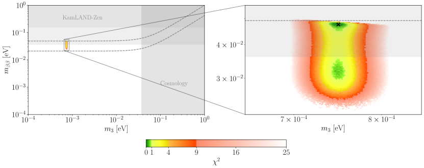
Figure 2: The effective neutrino mass for neutrinoless double beta decay as a function of the lightest neutrino mass. The experimentally allowed region within $3\sigma$ for inverted ordering is the region between the two dashed lines, while the region allowed in our model is represented by the colored area. The gray-shaded areas are excluded by KamLAND-Zen [111] or cosmological bounds [112, 109]. We remark that the KamLAND-Zen upper limit for the effective neutrino mass $m_{\beta\beta}$ depends on the used nuclear matrix element estimate. While all estimates applied by the KamLAND-Zen collaboration give rise to an upper bound of the effective mass to be below $156\,$meV (dark gray area), only some estimates yield limits that are smaller than $36\,$meV (light gray area) [111]. Hence, we find that the sample point marked by $\mathsf{x}$ is only challenged by some nuclear matrix element estimates while still being allowed according to the majority of estimates.

We remark that the model can be consistent with both octants of $\theta_{23}$, while only being compatible with Dirac $\mathcal{CP}$-violating phases in the range of $1.36<\delta_{\mathcal{CP}}^{\ell}<1.55$ at a $3\sigma$ C.L., as shown in Figure 3. Moreover, the inverted-ordering neutrino masses are predicted to lie within the narrow ranges

$$48\,\mathrm{meV}<m_{1}<50\,\mathrm{meV}\;,\quad 49\,\mathrm{meV}<m_{2}<51\,\mathrm{meV}\;,\quad 0.72\,\mathrm{meV}<m_{3}<0.78\,\mathrm{meV}\;,$$ (39)

at a $3\sigma$ C.L. The numerical analysis suggests that the model prefers a neutrino spectrum with inverted ordering. For a normal-ordering spectrum we only obtain a match with experimental data just barely in the $3\sigma$ interval with $\chi^{2}\approx 7$.

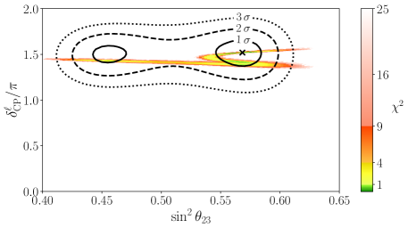
Figure 3: Predicted regions in the space of $\sin^{2}\theta_{23}$ and $\delta_{\mathcal{CP}}^{\ell}$ with $\chi^{2}\leq 25$ in our model. The black lines indicate the regions that are experimentally admissible at a $1$, $2$, and $3\sigma$ C.L. as obtained by the global analysis NuFIT v5.3 [106].

5 DM abundance

Let us start by identifying the DM candidate. Since the flavon field only couples to charged leptons, the phenomenological implications for DM in our model are determined by the charged-lepton Yukawa interactions and the flavon potential. The interactions between the SM charged leptons and the flavon scalar $\phi_{3}$ are given by

$$\mathcal{L}_{\mathrm{CL}} \leavevmode\nobreak\ =\leavevmode\nobreak\ -\sum_{i=1}^{3}\frac{v_{d}}{2}\alpha_{i}\,\psi_{E_{i}^{C}}\left(\psi_{E}\phi_{3}\right)_{{\boldsymbol{1}}}+\text{h.c}\;$$ (40)

$$\leavevmode\nobreak\ \longrightarrow\leavevmode\nobreak\ -\sum_{i=1}^{3}\frac{v_{d}}{2}\alpha_{i}\,\psi_{E_{i}^{C}}\left(\psi_{E}\left(\phi_{3}+v_{3}(1,a,b)^{T}\right)\right)_{{\boldsymbol{1}}}+\text{h.c.}\;,$$

where $\psi_{E}$ denotes the fermionic part of the charged-lepton component of $L$. In the last line, we develop the flavon $\phi_{3}$ in the vacuum with its VEV given by $v_{3}(1,a,b)^{T}$, see Equation 27. From the leading flavon superpotential terms in Equation 23, we obtain

$$\mathcal{L}_{\phi} \leavevmode\nobreak\ =\leavevmode\nobreak\ -\frac{1}{2}\Lambda_{\phi}\beta_{1}\left(\psi_{\zeta_{3}}\psi_{\phi_{3}}\right)_{{\boldsymbol{1}}}-\frac{1}{2}\beta_{2}\left(\psi_{\zeta_{3}}\psi_{\phi_{3}}\phi_{3}\right)_{{\boldsymbol{1}}}-\frac{1}{2}\Lambda_{\phi}\beta_{4}\left(\psi_{\zeta_{1^{\prime\prime}}}\psi_{\phi_{1^{\prime}}}\right)_{{\boldsymbol{1}}}+\text{h.c.}$$ (41)

$$\leavevmode\nobreak\ \to\leavevmode\nobreak\ -\frac{1}{2}\Lambda_{\phi}\beta_{1}\left(\psi_{\zeta_{3}}\psi_{\phi_{3}}\right)_{{\boldsymbol{1}}}-\frac{1}{2}\beta_{2}\left(\psi_{\zeta_{3}}\psi_{\phi_{3}}\left(\phi_{3}+v_{3}(1,a,b)^{T}\right)\right)_{{\boldsymbol{1}}}$$

$$\leavevmode\nobreak\ \leavevmode\nobreak\ \leavevmode\nobreak\ \leavevmode\nobreak\ \leavevmode\nobreak\ -\frac{1}{2}\Lambda_{\phi}\beta_{4}\left(\psi_{\zeta_{1^{\prime\prime}}}\psi_{\phi_{1^{\prime}}}\right)_{{\boldsymbol{1}}}+\text{h.c.}$$

$$\leavevmode\nobreak\ =\leavevmode\nobreak\ -\frac{1}{2}\Lambda_{\phi}\beta_{1}\left(\psi_{\zeta_{3}}\psi_{\phi_{3}}\right)_{{\boldsymbol{1}}}-\frac{4.27}{2}\beta_{1}\left(\psi_{\zeta_{3}}\psi_{\phi_{3}}\left(\phi_{3}+v_{3}(1,a,b)^{T}\right)\right)_{{\boldsymbol{1}}}$$

$$\leavevmode\nobreak\ \leavevmode\nobreak\ \leavevmode\nobreak\ \leavevmode\nobreak\ \leavevmode\nobreak\ -\frac{1}{2}\Lambda_{\phi}\beta_{4}\left(\psi_{\zeta_{1^{\prime\prime}}}\psi_{\phi_{1^{\prime}}}\right)_{{\boldsymbol{1}}}+\text{h.c.}\,,$$

where $\phi_{3}$ is again expanded around its VEV in the second line and we use the relations of Equation 36 in the last line.

The DM candidate is the lowest mass-state Dirac fermion built as a linear combination of the Weyl components of the driving fields and flavon fields, $\psi_{\zeta_{i}},\psi_{\phi_{i}}$, whereas the mediator is a linear combination of the flavon scalars. The particle content relevant for DM production is outlined in Table 4. After the Higgs and the flavons acquire VEVs as given in Equation 27, the symmetry group of Table 2 gets broken down to $\mathrm{U}(1)_{\text{EM}}\times\mathrm{U}(1)_{R}$.

	$\psi_{E_{i}}$	$\psi_{E_{i}^{C}}$	$\phi_{3,i}$	$\phi_{1^{\prime}}$	$\psi_{\phi_{3,i}}$	$\psi_{\zeta_{3,i}}$	$\psi_{\phi_{1^{\prime}}}$	$\psi_{\zeta_{1^{\prime\prime}}}$
$\mathrm{U}(1)_{\text{EM}}$	$-1$	$+1$	$0$	$0$	$0$	$0$	$0$	$0$
$\mathrm{U}(1)_{R}$	$0$	$0$	$0$	$0$	$-1$	$+1$	$-1$	$+1$

Table 4: Particle content for DM production.

Interactions in Equations 40 and 41 allow for processes as shown in the diagrams in Figure 4(a). Furthermore, we also consider the scalar potential

$$V=\frac{\partial W}{\partial\varphi_{i}}K^{i\bar{\jmath}}\frac{\partial W^{*}}{\partial\varphi_{\bar{\jmath}}^{*}}+\sum_{i=1,2,3}|\widetilde{m}_{\phi}\phi_{3,i}|^{2}+|\widetilde{m}_{\phi}\phi_{1^{\prime}}|^{2}\;,$$ (42)

where we have added the soft-masses $\widetilde{m}_{\phi}$ for the flavon scalars. We assume that $\widetilde{m}_{\phi}$ is the same for the four scalars and should be of order of the SUSY breaking scale. It has been shown in [114] that for modular $A_{4}$ supersymmetric models, the SUSY breaking scale is constrained to be above $6$ TeV. Therefore, we choose values of order $\widetilde{m}_{\phi}=20-1000$ TeV. Furthermore, the $A$-term in Equation 20 does not play a significant role in DM production at tree-level since the production of DM through flavon scalar annihilations are suppressed due to the low reheating temperature we consider; therefore, we also ignore the $A$-term in our analysis.

(a) DM production diagram.

(b) Effective DM production diagram

Figure 4: (a). The indices $i,j,m$ indicate the three possible charged-lepton flavor states, while the indices $n,k,\ell$ indicate the three possible components of the triplet plus the non-trivial singlet of flavons and driving fields. DM is identified as the lowest mass-state of $\psi_{\zeta_{\ell}},\psi_{\phi_{n}}$. The mediator is the scalar flavon $\phi_{k}$. (b) Since the effective mass of the flavon scalar is expected to be very big, $m_{\phi}\gg m_{E_{i}},m_{\psi_{\phi\zeta}}$, then the diagram shrinks to an effective $4-$fermion interaction. This leads to a preferred freeze-in scenario.

It turns out that the correct DM relic abundance can be obtained with a freeze-in scenario [115] in this model (cf. [99] where a freeze-out production mechanism is utilized). This can be seen as follows. First, note that the effective scalar flavon mass $m_{\phi}$ is obtained by diagonalizing the mass matrix obtained from Equation 42. If we assume that $\widetilde{m}_{\phi}\gg m_{E_{i}},m_{\psi_{\phi\zeta}}$, where $m_{E_{i}},m_{\psi_{\phi\zeta}}=m_{\text{DM}}\sim\Lambda_{\phi}\beta_{1}$ represent the mass of the charged leptons and the DM respectively, then the mediator mass ($m_{\phi}\sim\widetilde{m}_{\phi}+m_{\psi_{\phi\zeta}}$) is much larger than the DM and the charged-lepton masses. Therefore, the diagram Figure 4(a) reduces to the effective $4-$fermion operator as indicated in Figure 4(b) with a coupling of $\sim\frac{\beta_{2}\alpha_{m}}{m_{\phi}^{2}}$. In a freeze-out mechanism, if the rate $\left\langle\sigma v\right\rangle$ at which DM is annihilated decreases, then the amount of DM relic abundance increases. Since we must require $\beta_{2}\ll 4\pi$ to retain perturbativity, and we expect $\alpha_{1}=-6.97$, as explained at the end Section 4, then

$$\left\langle\sigma v\right\rangle\sim\left|\frac{\beta_{2}\alpha_{m}}{m_{\phi}^{2}}\right|^{2}\ll\left|\frac{88}{m_{\phi}^{2}}\right|^{2}\;.$$ (43)

Using micrOMEGAs 5.3.41 [116, 117, 118], we find that for the chosen values of $\Lambda_{\phi}$ and $\widetilde{m}_{\phi}$, too much DM is produced. Since increasing $m_{\phi}$ or lowering $\beta_{2}$ would only decrease $\left\langle\sigma v\right\rangle$, the DM abundance can not be decreased to the observed DM abundance in a freeze-out scenario. On the other hand, for a freeze-in scenario, we have the opposite behavior. Specifically, if $\left\langle\sigma v\right\rangle$ decreases, the amount of produced DM also decreases. So, we can choose smaller $\beta_{2}$ or larger $m_{\phi}$ values to obtain the observed relic abundance of DM in the Universe.

We now proceed to present the predictions of our model for the DM abundance after performing a parameter scan. We use micrOMEGAs 5.3.41 [116, 117, 118] for the DM abundance computation and FeynRules 2.0 [119] to create the CalcHEP [120] model files. As mentioned earlier, we assume $\tan\beta=60$ and a low reheating temperature of $T_{\text{R}}=150$ GeV.

From our discussion we see that we have 4 free parameters to determine the DM in our model:

1. the scalar flavon soft-mass $\widetilde{m}_{\phi}$,

2. the flavor breaking scale $\Lambda_{\phi}$,

3. the coupling $\beta_{1}$ in Equation 23, and

4. the coupling $\beta_{4}$ in Equation 23.

We fix $10^{-6}\leq\beta_{1},\beta_{4}\leq 10^{-4}$ and $20$ TeV $\leq\widetilde{m}_{\phi},\,\Lambda_{\phi}\leq 1000$ TeV. These bounds for the couplings $\beta_{1},\,\beta_{4}$ respect the perturbativity of all the couplings $\beta_{i}$ (cf. Equation 36).

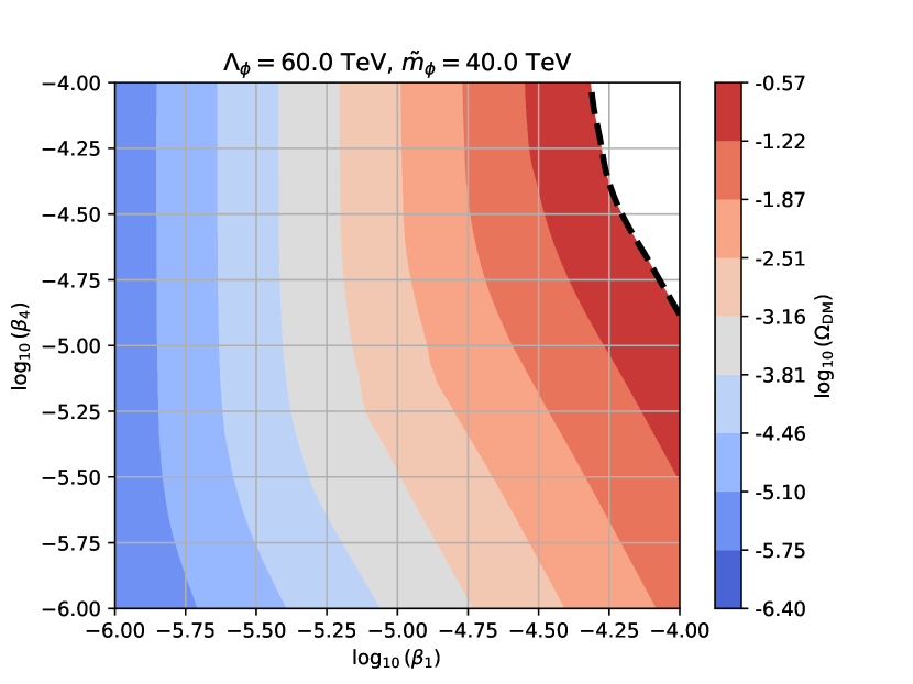
(a)

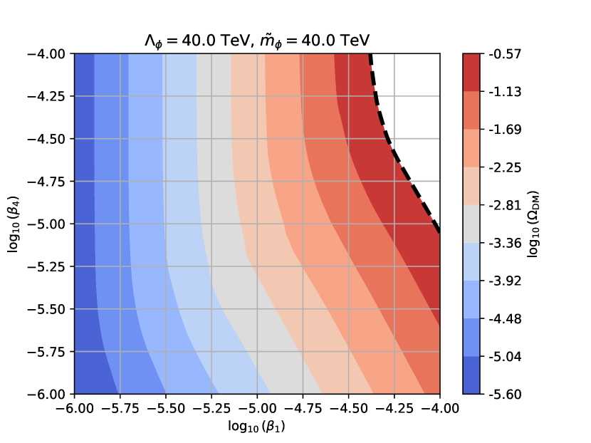
(b)

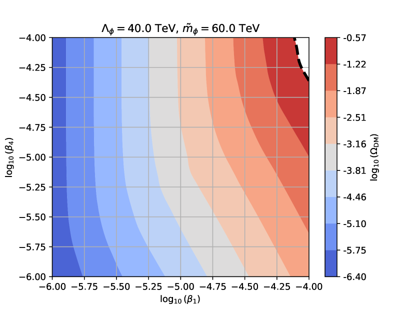
(c)

Figure 5: Predicted DM relic abundance as a function of $\log_{10}\left(\beta_{1}\right)$ and $\log_{10}\left(\beta_{4}\right)$ with fixed values of $\widetilde{m}_{\phi}$ and $\Lambda_{\phi}$ at some benchmark values. We choose $T_{\text{R}}=150$ GeV. The dashed black line denotes the relic DM abundance $\Omega_{\text{DM}}=0.265$.

In Figure 5 we show the prediction for DM relic abundance as a function of $\beta_{1}$ and $\beta_{4}$, for $\Lambda_{\phi}>\widetilde{m}_{\phi}$ (Figure 5(a)), $\widetilde{m}_{\phi}=\Lambda_{\phi}$ (Figure 5(b)), and $\widetilde{m}_{\phi}<\Lambda_{\phi}$ (Figure 5(c)). The unshaded region indicates the excluded parameter space where too much DM is produced. We see that all plots in Figure 5 exhibit similar behavior. It is possible to have a coupling up to $\beta_{4},\beta_{1}=10^{-4}$, but not at the same time. This is consistent with the fact that freeze-in normally requires small couplings [115]. Furthermore, the abundance increases as we increase either $\beta_{1}$ or $\beta_{4}$, which is consistent with the fact that the DM relic abundance increases with $\left\langle\sigma v\right\rangle$.

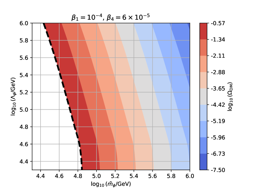
(a)

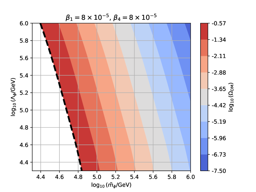
(b)

(c)

Figure 6: Predicted DM relic abundance as a function of $\log_{10}\left(\widetilde{m}_{\phi}/\text{GeV}\right)$ and $\log_{10}\left(\Lambda_{\phi}/\text{GeV}\right)$ with fixed values of $\beta_{1}$ and $\beta_{4}$ at some benchmark values. We choose $T_{\text{R}}=150$ GeV. The dashed black line denotes the relic DM abundance $\Omega_{\text{DM}}=0.265$.

Figure 6 shows the predicted DM relic abundance as a function of $\widetilde{m}_{\phi}$ and $\Lambda_{\phi}$ for $\beta_{1}>\beta_{4}$ (Figure 6(a)), $\beta_{1}=\beta_{4}$ (Figure 6(b)), and $\beta_{1}<\beta_{4}$ (Figure 6(c)). The unshaded space represents the excluded parameter space. We observe a similar behavior for the three plots in Figure 6. The DM abundance decreases if either $\widetilde{m}_{\phi}$ or $\Lambda_{\phi}$ grows. Furthermore, a soft-mass of $m_{\phi}=20$ TeV and a simultaneous flavon breaking-scale $\Lambda_{\phi}=20$ TeV is excluded in all cases for the chosen values of other parameters.

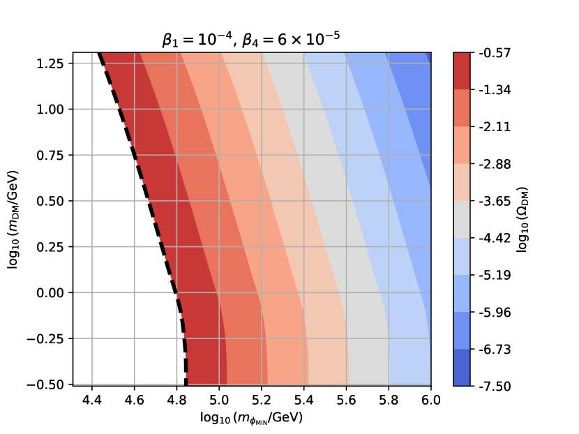
(a)

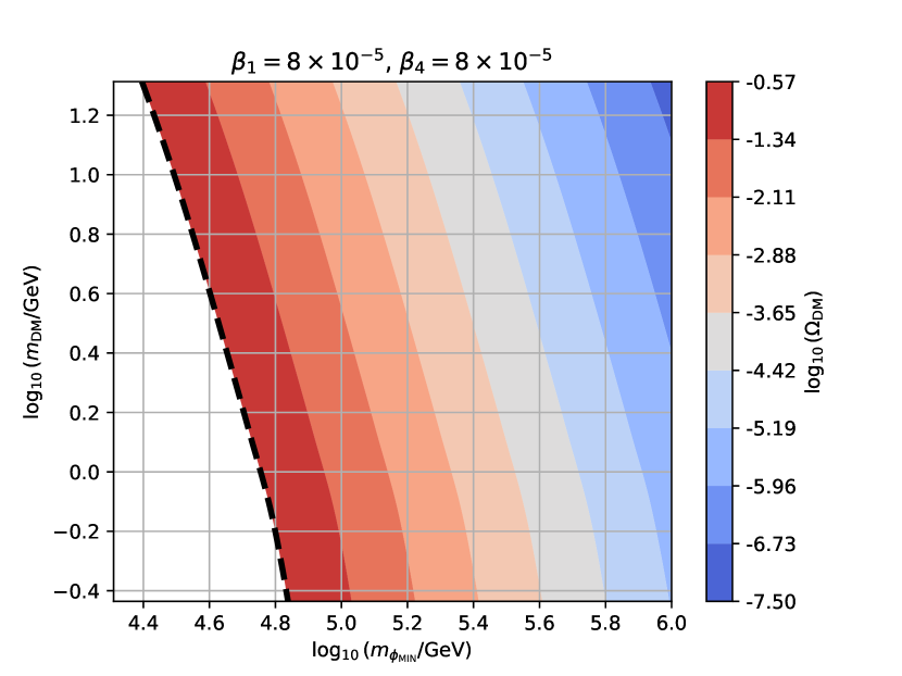
(b)

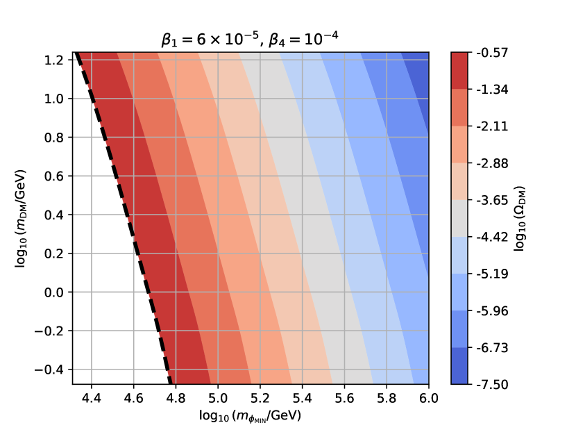
(c)

Figure 7: Predicted DM relic abundance as a function of the minimum mediator scalar flavon mass $\log_{10}\left(m_{\phi_{\text{MIN}}}/\text{GeV}\right)$ and DM mass $\log_{10}\left(m_{\text{DM}}/\text{GeV}\right)$ for fixed $\beta_{1}$ and $\beta_{4}$ at some benchmark values. We fix $T_{\text{R}}=150\text{ GeV}$. The dashed black line denotes the relic DM abundance $\Omega_{\text{DM}}=0.265$.

Finally, in Figure 7 we show the correlation between the minimum scalar flavon mass $m_{\phi_{\text{MIN}}}$ and DM mass $m_{\text{DM}}$ for fixed values of $\beta_{1}>\beta_{4}$ (Figure 7(a)), $\beta_{1}=\beta_{4}$ (Figure 7(b)), and $\beta_{1}<\beta_{4}$ (Figure 7(c)). By comparing Figures 7 and 6, we find that for a given value of the soft-mass $\widetilde{m}_{\phi}$, the minimum scalar flavon mass $m_{\phi_{\text{MIN}}}$ constrained by the DM relic abundance can be derived. We see that the scalar flavon mass can be as low as $\sim 63$ TeV for all cases illustrated in Figure 7. Moreover, the DM mass can be as low as $\sim 16$ GeV for $\beta_{1}=6\times 10^{-5}$ and $\beta_{4}=10^{-4}$.

6 Conclusion

We constructed a flavor model based on the finite modular group $\Gamma_{3}\cong A_{4}$ that simultaneously explains the flavor parameters in the lepton sector and accounts for the observed DM relic abundance in the Universe. The 12 lepton flavor parameters are determined by 8 real parameters: the two components of the modulus VEV, the four flavon VEVs, $\left\langle\phi_{i}\right\rangle$, and two dimensionful parameters that set the mass scales of charged-lepton and neutrino masses. We identify a DM candidate composed of the fermionic parts of the flavon superfields and the driving superfields. The mediator is the scalar part of the flavon superfield which interacts with the charged-lepton sector of the SM. We obtain a good fit to the lepton flavor parameters (3 charged lepton masses, 3 mixing angles, 1 $\mathcal{CP}$ phase, 2 neutrino squared mass differences) with $\chi^{2}=0.08$ for an inverted-hierarchy neutrino spectrum. The lepton flavor fit fixes the couplings of the charged leptons to the DM mediator as well as the flavon VEVs $\left\langle\phi_{i}\right\rangle$. These VEVs satisfy the $F$-term equations to retain supersymmetry at high energies, determining thereby the coupling between our DM candidate and the mediator. Interestingly, our model exhibits 4 additional degrees of freedom that are left free and serve to achieve a DM relic abundance which does not exceed the observed value $\Omega_{\text{CDM}}=0.265$. These parameters are 2 dimensionless couplings $\beta_{1},\beta_{4}$, the flavor breaking scale $\Lambda_{\phi}$, and the soft-mass for the flavon $\widetilde{m}_{\phi}$. We find that if the mediator mass is assumed to be much larger than the DM and the charged-lepton masses, then the appropriate DM production mechanism is freeze-in rather than freeze-out. We observe that a viable DM relic abundance can be generated in regions of the parameter space constrained by $10^{-6}\leq\beta_{1},\beta_{4}\leq 10^{-4}$, $20$ TeV $\leq\widetilde{m}_{\phi},\,\Lambda_{\phi}\leq 1000$ TeV, $\tan\beta=60$, and $T_{R}=150$ GeV.

Although some amount of tuning is necessary in our model to identify the best parameter values, we point out that it is the choice of charges and modular weights that render the right flavon superpotential, which in turn delivers the alignment of the flavon VEVs $\left\langle\phi_{i}\right\rangle$. Further, the phenomenologically viable value of the modulus VEV $\left\langle\tau\right\rangle$ might be achieved through mechanisms as in [97].

As a feasible outlook of our findings, it would be interesting to study the possibility of applying this new scenario in top-down models such as [88]. Another interesting aspect to explore would be the study of additional constraints on the DM free parameters $\beta_{1},\,\beta_{4},\,\Lambda_{\phi}$ and $\widetilde{m}_{\phi}$. This could be done by using constraints from electron scattering searches like XENON1T [121], SENSEI [122] or DAMIC [123]. Furthermore, this model only accounts for the lepton sector, but it should be extended to the quark sector. In this case, we could also use searches from nucleon scattering like LUX [124], DEAP-3600 [125], PandaX-II [126], DarkSide [127] or EDELWEISS [128]. We leave these intriguing questions for upcoming work.

Acknowledgments

The work of M.-C.C. and V.K.-P. was partially supported by the U.S. National Science Foundation under Grant No. PHY-1915005. The work of S.R.-S. was partly supported by UNAM-PAPIIT grant IN113223 and Marcos Moshinsky Foundation. This work was also supported by UC-MEXUS-CONACyT grant No. CN-20-38. V.K.-P. would like to thank Kevork N. Abazajian, Max Fieg, Xueqi Li, Xiang-Gan Liu, Gopolang Mohlabeng, Michael Ratz and Miša Toman for fruitful discussions. M-C.C.and V.K.-P. would also like to thank Instituto de Física, UNAM, for the hospitality during their visit. A.B. would like to thank the Department of Physics and Astronomy at UCI for the hospitality during his visit. V.K.-P. also thanks the opportunity to use the cluster at Instituto de Física, UNAM. This work utilized the infrastructure for high-performance and high-throughput computing, research data storage and analysis, and scientific software tool integration built, operated, and updated by the Research Cyberinfrastructure Center (RCIC) at the University of California, Irvine (UCI). The RCIC provides cluster-based systems, application software, and scalable storage to directly support the UCI research community. https://rcic.uci.edu

References

• [1] G. Altarelli and F. Feruglio, Rev. Mod. Phys. 82 (2010), 2701, arXiv:1002.0211 [hep-ph].
• [2] H. Ishimori, T. Kobayashi, H. Ohki, Y. Shimizu, H. Okada, and M. Tanimoto, Prog. Theor. Phys. Suppl. 183 (2010), 1, arXiv:1003.3552 [hep-th].
• [3] D. Hernández and A. Y. Smirnov, Phys. Rev. D 86 (2012), 053014, arXiv:1204.0445 [hep-ph].
• [4] S. F. King and C. Luhn, Rept. Prog. Phys. 76 (2013), 056201, arXiv:1301.1340 [hep-ph].
• [5] S. F. King, A. Merle, S. Morisi, Y. Shimizu, and M. Tanimoto, New J. Phys. 16 (2014), 045018, arXiv:1402.4271 [hep-ph].
• [6] S. F. King, Prog. Part. Nucl. Phys. 94 (2017), 217, arXiv:1701.04413 [hep-ph].
• [7] F. Feruglio and A. Romanino, Rev. Mod. Phys. 93 (2021), no. 1, 015007, arXiv:1912.06028 [hep-ph].
• [8] G. Altarelli and F. Feruglio, Nucl. Phys. B 741 (2006), 215, hep-ph/0512103.
• [9] F. Feruglio, C. Hagedorn, and L. Merlo, JHEP 03 (2010), 084, arXiv:0910.4058 [hep-ph].
• [10] G.-J. Ding, S. F. King, C. Luhn, and A. J. Stuart, JHEP 05 (2013), 084, arXiv:1303.6180 [hep-ph].
• [11] C.-C. Li and G.-J. Ding, Nucl. Phys. B 881 (2014), 206, arXiv:1312.4401 [hep-ph].
• [12] Y. Muramatsu, T. Nomura, and Y. Shimizu, JHEP 03 (2016), 192, arXiv:1601.04788 [hep-ph].
• [13] S. F. King and Y.-L. Zhou, JHEP 05 (2019), 217, arXiv:1901.06877 [hep-ph].
• [14] A. E. Cárcamo Hernández and S. F. King, Nucl. Phys. B 953 (2020), 114950, arXiv:1903.02565 [hep-ph].
• [15] M.-C. Chen, V. Knapp-Pérez, M. Ramos-Hamud, S. Ramos-Sánchez, M. Ratz, and S. Shukla, Phys. Lett. B 824 (2022), 136843, arXiv:2108.02240 [hep-ph].
• [16] M. Hirsch, S. Morisi, E. Peinado, and J. W. F. Valle, Phys. Rev. D 82 (2010), 116003, arXiv:1007.0871 [hep-ph].
• [17] X.-G. He, X.-D. Ma, M. A. Schmidt, G. Valencia, and R. R. Volkas, arXiv:2403.12485 [hep-ph].
• [18] H. Acaroğlu, M. Blanke, J. Heisig, M. Krämer, and L. Rathmann, JHEP 06 (2024), 179, arXiv:2312.09274 [hep-ph].
• [19] H. Acaroğlu and M. Blanke, JHEP 05 (2022), 086, arXiv:2109.10357 [hep-ph].
• [20] F. Feruglio, Are neutrino masses modular forms?, 227, 2019, pp. 227–266.
• [21] J. C. Criado and F. Feruglio, SciPost Phys. 5 (2018), no. 5, 042, arXiv:1807.01125 [hep-ph].
• [22] T. Kobayashi, K. Tanaka, and T. H. Tatsuishi, Phys. Rev. D 98 (2018), no. 1, 016004, arXiv:1803.10391 [hep-ph].
• [23] F. J. de Anda, S. F. King, and E. Perdomo, Phys. Rev. D 101 (2020), no. 1, 015028, arXiv:1812.05620 [hep-ph].
• [24] H. Okada and M. Tanimoto, Phys. Lett. B 791 (2019), 54, arXiv:1812.09677 [hep-ph].
• [25] G.-J. Ding, S. F. King, and X.-G. Liu, Phys. Rev. D 100 (2019), no. 11, 115005, arXiv:1903.12588 [hep-ph].
• [26] T. Kobayashi, Y. Shimizu, K. Takagi, M. Tanimoto, and T. H. Tatsuishi, Phys. Rev. D 100 (2019), no. 11, 115045, arXiv:1909.05139 [hep-ph], [Erratum: Phys.Rev.D 101, 039904 (2020)].
• [27] T. Asaka, Y. Heo, T. H. Tatsuishi, and T. Yoshida, JHEP 01 (2020), 144, arXiv:1909.06520 [hep-ph].
• [28] X.-G. Liu and G.-J. Ding, JHEP 08 (2019), 134, arXiv:1907.01488 [hep-ph].
• [29] G.-J. Ding and S. F. King, Rept. Prog. Phys. 87 (2024), no. 8, 084201, arXiv:2311.09282 [hep-ph].
• [30] T. Kobayashi, N. Omoto, Y. Shimizu, K. Takagi, M. Tanimoto, and T. H. Tatsuishi, JHEP 11 (2018), 196, arXiv:1808.03012 [hep-ph].
• [31] P. P. Novichkov, J. T. Penedo, S. T. Petcov, and A. V. Titov, JHEP 04 (2019), 174, arXiv:1812.02158 [hep-ph].
• [32] P. P. Novichkov, J. T. Penedo, S. T. Petcov, and A. V. Titov, JHEP 04 (2019), 005, arXiv:1811.04933 [hep-ph].
• [33] P. P. Novichkov, S. T. Petcov, and M. Tanimoto, Phys. Lett. B 793 (2019), 247, arXiv:1812.11289 [hep-ph].
• [34] J. T. Penedo and S. T. Petcov, Nucl. Phys. B 939 (2019), 292, arXiv:1806.11040 [hep-ph].
• [35] J. C. Criado, F. Feruglio, and S. J. D. King, JHEP 02 (2020), 001, arXiv:1908.11867 [hep-ph].
• [36] G.-J. Ding, S. F. King, and X.-G. Liu, JHEP 09 (2019), 074, arXiv:1907.11714 [hep-ph].
• [37] T. Kobayashi, Y. Shimizu, K. Takagi, M. Tanimoto, and T. H. Tatsuishi, JHEP 02 (2020), 097, arXiv:1907.09141 [hep-ph].
• [38] G.-J. Ding, S. F. King, C.-C. Li, and Y.-L. Zhou, JHEP 08 (2020), 164, arXiv:2004.12662 [hep-ph].
• [39] P. P. Novichkov, J. T. Penedo, and S. T. Petcov, Nucl. Phys. B 963 (2021), 115301, arXiv:2006.03058 [hep-ph].
• [40] X. Wang, B. Yu, and S. Zhou, Phys. Rev. D 103 (2021), no. 7, 076005, arXiv:2010.10159 [hep-ph].
• [41] C.-C. Li, X.-G. Liu, and G.-J. Ding, JHEP 10 (2021), 238, arXiv:2108.02181 [hep-ph].
• [42] T. Kobayashi, Y. Shimizu, K. Takagi, M. Tanimoto, and T. H. Tatsuishi, PTEP 2020 (2020), no. 5, 053B05, arXiv:1906.10341 [hep-ph].
• [43] G.-J. Ding, F. Feruglio, and X.-G. Liu, JHEP 01 (2021), 037, arXiv:2010.07952 [hep-th].
• [44] J.-N. Lu, X.-G. Liu, and G.-J. Ding, Phys. Rev. D 101 (2020), no. 11, 115020, arXiv:1912.07573 [hep-ph].
• [45] S. J. D. King and S. F. King, JHEP 09 (2020), 043, arXiv:2002.00969 [hep-ph].
• [46] X.-G. Liu, C.-Y. Yao, and G.-J. Ding, Phys. Rev. D 103 (2021), no. 5, 056013, arXiv:2006.10722 [hep-ph].
• [47] H. Okada and M. Tanimoto, Phys. Rev. D 103 (2021), no. 1, 015005, arXiv:2009.14242 [hep-ph].
• [48] P. Chen, G.-J. Ding, and S. F. King, JHEP 04 (2021), 239, arXiv:2101.12724 [hep-ph].
• [49] G.-J. Ding, S. F. King, and J.-N. Lu, JHEP 11 (2021), 007, arXiv:2108.09655 [hep-ph].
• [50] Y. Zhao and H.-H. Zhang, JHEP 03 (2021), 002, arXiv:2101.02266 [hep-ph].
• [51] C. Arriaga-Osante, X.-G. Liu, and S. Ramos-Sánchez, JHEP 05 (2024), 119, arXiv:2311.10136 [hep-ph].
• [52] S. Kikuchi, T. Kobayashi, K. Nasu, S. Takada, and H. Uchida, JHEP 07 (2023), 134, arXiv:2302.03326 [hep-ph].
• [53] S. Kikuchi, T. Kobayashi, K. Nasu, S. Takada, and H. Uchida, JHEP 04 (2024), 045, arXiv:2310.17978 [hep-ph].
• [54] F. Feruglio, V. Gherardi, A. Romanino, and A. Titov, JHEP 05 (2021), 242, arXiv:2101.08718 [hep-ph].
• [55] F. Feruglio, Phys. Rev. Lett. 130 (2023), no. 10, 101801, arXiv:2211.00659 [hep-ph].
• [56] S. T. Petcov and M. Tanimoto, Eur. Phys. J. C 83 (2023), no. 7, 579, arXiv:2212.13336 [hep-ph].
• [57] Y. Abe, T. Higaki, J. Kawamura, and T. Kobayashi, Eur. Phys. J. C 83 (2023), no. 12, 1140, arXiv:2301.07439 [hep-ph].
• [58] F. Feruglio, JHEP 03 (2023), 236, arXiv:2302.11580 [hep-ph].
• [59] T. Nomura and H. Okada, Phys. Lett. B 797 (2019), 134799, arXiv:1904.03937 [hep-ph].
• [60] M. K. Behera, S. Singirala, S. Mishra, and R. Mohanta, J. Phys. G 49 (2022), no. 3, 035002, arXiv:2009.01806 [hep-ph].
• [61] P. T. P. Hutauruk, D. W. Kang, J. Kim, and H. Okada, Phys. Dark Univ. 44 (2024), 101440, arXiv:2012.11156 [hep-ph].
• [62] T. Kobayashi, H. Okada, and Y. Orikasa, Phys. Dark Univ. 37 (2022), 101080, arXiv:2111.05674 [hep-ph].
• [63] X. Zhang and S. Zhou, JCAP 09 (2021), 043, arXiv:2106.03433 [hep-ph].
• [64] T. Kobayashi, S. Nagamoto, and S. Uemura, PTEP 2017 (2017), no. 2, 023B02, arXiv:1608.06129 [hep-th].
• [65] T. Kobayashi, S. Nagamoto, S. Takada, S. Tamba, and T. H. Tatsuishi, Phys. Rev. D 97 (2018), no. 11, 116002, arXiv:1804.06644 [hep-th].
• [66] T. Kobayashi and S. Tamba, Phys. Rev. D 99 (2019), no. 4, 046001, arXiv:1811.11384 [hep-th].
• [67] Y. Kariyazono, T. Kobayashi, S. Takada, S. Tamba, and H. Uchida, Phys. Rev. D 100 (2019), no. 4, 045014, arXiv:1904.07546 [hep-th].
• [68] K. Hoshiya, S. Kikuchi, T. Kobayashi, Y. Ogawa, and H. Uchida, PTEP 2021 (2021), no. 3, 033B05, arXiv:2012.00751 [hep-th].
• [69] S. Kikuchi, T. Kobayashi, S. Takada, T. H. Tatsuishi, and H. Uchida, Phys. Rev. D 102 (2020), no. 10, 105010, arXiv:2005.12642 [hep-th].
• [70] S. Kikuchi, T. Kobayashi, H. Otsuka, S. Takada, and H. Uchida, JHEP 11 (2020), 101, arXiv:2007.06188 [hep-th].
• [71] H. Ohki, S. Uemura, and R. Watanabe, Phys. Rev. D 102 (2020), no. 8, 085008, arXiv:2003.04174 [hep-th].
• [72] Y. Almumin, M.-C. Chen, V. Knapp-Pérez, S. Ramos-Sánchez, M. Ratz, and S. Shukla, JHEP 05 (2021), 078, arXiv:2102.11286 [hep-th].
• [73] S. Kikuchi, T. Kobayashi, and H. Uchida, Phys. Rev. D 104 (2021), no. 6, 065008, arXiv:2101.00826 [hep-th].
• [74] Y. Tatsuta, JHEP 10 (2021), 054, arXiv:2104.03855 [hep-th].
• [75] S. Kikuchi, T. Kobayashi, K. Nasu, H. Uchida, and S. Uemura, Phys. Rev. D 105 (2022), no. 11, 116002, arXiv:2202.05425 [hep-th].
• [76] S. Kikuchi, T. Kobayashi, K. Nasu, and H. Uchida, JHEP 08 (2022), 256, arXiv:2203.01649 [hep-th].
• [77] S. Kikuchi, T. Kobayashi, K. Nasu, S. Takada, and H. Uchida, JHEP 06 (2023), 013, arXiv:2211.07813 [hep-th].
• [78] A. Baur, H. P. Nilles, A. Trautner, and P. K. S. Vaudrevange, Phys. Lett. B 795 (2019), 7, arXiv:1901.03251 [hep-th].
• [79] A. Baur, H. P. Nilles, A. Trautner, and P. K. S. Vaudrevange, Nucl. Phys. B 947 (2019), 114737, arXiv:1908.00805 [hep-th].
• [80] H. P. Nilles, S. Ramos-Sánchez, and P. K. S. Vaudrevange, Nucl. Phys. B 957 (2020), 115098, arXiv:2004.05200 [hep-ph].
• [81] H. P. Nilles, S. Ramos-Sánchez, and P. K. S. Vaudrevange, Phys. Lett. B 808 (2020), 135615, arXiv:2006.03059 [hep-th].
• [82] A. Baur, M. Kade, H. P. Nilles, S. Ramos-Sánchez, and P. K. S. Vaudrevange, JHEP 02 (2021), 018, arXiv:2008.07534 [hep-th].
• [83] H. P. Nilles, S. Ramos–Sánchez, and P. K. S. Vaudrevange, Nucl. Phys. B 966 (2021), 115367, arXiv:2010.13798 [hep-th].
• [84] A. Baur, M. Kade, H. P. Nilles, S. Ramos-Sánchez, and P. K. S. Vaudrevange, Phys. Lett. B 816 (2021), 136176, arXiv:2012.09586 [hep-th].
• [85] A. Baur, M. Kade, H. P. Nilles, S. Ramos-Sánchez, and P. K. S. Vaudrevange, JHEP 06 (2021), 110, arXiv:2104.03981 [hep-th].
• [86] H. P. Nilles, S. Ramos-Sánchez, A. Trautner, and P. K. S. Vaudrevange, Nucl. Phys. B 971 (2021), 115534, arXiv:2105.08078 [hep-th].
• [87] A. Baur, H. P. Nilles, S. Ramos-Sánchez, A. Trautner, and P. K. S. Vaudrevange, Phys. Rev. D 105 (2022), no. 5, 055018, arXiv:2112.06940 [hep-th].
• [88] A. Baur, H. P. Nilles, S. Ramos-Sánchez, A. Trautner, and P. K. S. Vaudrevange, JHEP 09 (2022), 224, arXiv:2207.10677 [hep-ph].
• [89] A. Baur, H. P. Nilles, S. Ramos-Sánchez, A. Trautner, and P. K. S. Vaudrevange, arXiv:2405.20378 [hep-th].
• [90] H. P. Nilles, S. Ramos-Sánchez, and P. K. S. Vaudrevange, JHEP 02 (2020), 045, arXiv:2001.01736 [hep-ph].
• [91] A. Font, L. E. Ibanez, D. Lust, and F. Quevedo, Phys. Lett. B 245 (1990), 401.
• [92] H. P. Nilles and M. Olechowski, Phys. Lett. B 248 (1990), 268.
• [93] M. Cvetic, A. Font, L. E. Ibanez, D. Lust, and F. Quevedo, Nucl. Phys. B 361 (1991), 194.
• [94] S. Kachru, R. Kallosh, A. D. Linde, and S. P. Trivedi, Phys. Rev. D 68 (2003), 046005, hep-th/0301240.
• [95] K. A. Intriligator, N. Seiberg, and D. Shih, JHEP 04 (2006), 021, hep-th/0602239.
• [96] J. M. Leedom, N. Righi, and A. Westphal, JHEP 02 (2023), 209, arXiv:2212.03876 [hep-th].
• [97] V. Knapp-Pérez, X.-G. Liu, H. P. Nilles, S. Ramos-Sánchez, and M. Ratz, Phys. Lett. B 844 (2023), 138106, arXiv:2304.14437 [hep-th].
• [98] Particle Data Group, P. A. Zyla et al., PTEP 2020 (2020), no. 8, 083C01.
• [99] T. Nomura, Y. Shimizu, and T. Takahashi, arXiv:2405.14163 [hep-ph].
• [100] X.-G. Liu, C.-Y. Yao, B.-Y. Qu, and G.-J. Ding, Phys. Rev. D 102 (2020), no. 11, 115035, arXiv:2007.13706 [hep-ph].
• [101] X.-G. Liu and G.-J. Ding, JHEP 03 (2022), 123, arXiv:2112.14761 [hep-ph].
• [102] M.-C. Chen, S. Ramos-Sánchez, and M. Ratz, Phys. Lett. B 801 (2020), 135153, arXiv:1909.06910 [hep-ph].
• [103] G.-J. Ding, X.-G. Liu, and C.-Y. Yao, JHEP 01 (2023), 125, arXiv:2211.04546 [hep-ph].
• [104] J. Terning, Modern supersymmetry: Dynamics and duality, 2006.
• [105] Particle Data Group, R. L. Workman and Others, PTEP 2022 (2022), 083C01.
• [106] I. Esteban, M. C. González-García, M. Maltoni, T. Schwetz, and A. Zhou, JHEP 09 (2020), 178, arXiv:2007.14792 [hep-ph], https://www.nu-fit.org.
• [107] S. Antusch and V. Maurer, JHEP 11 (2013), 115, arXiv:1306.6879 [hep-ph].
• [108] A. Baur, FlavorPy, 2024, https://doi.org/10.5281/zenodo.11060597.
• [109] Planck, N. Aghanim et al., Astron. Astrophys. 641 (2020), A6, arXiv:1807.06209 [astro-ph.CO], [Erratum: Astron.Astrophys. 652, C4 (2021)].
• [110] KATRIN, M. Aker et al., Nature Phys. 18 (2022), no. 2, 160, arXiv:2105.08533 [hep-ex].
• [111] KamLAND-Zen, S. Abe et al., Phys. Rev. Lett. 130 (2023), no. 5, 051801, arXiv:2203.02139 [hep-ex].
• [112] GAMBIT Cosmology Workgroup, P. Stöcker et al., Phys. Rev. D 103 (2021), no. 12, 123508, arXiv:2009.03287 [astro-ph.CO].
• [113] M. D’Onofrio and K. Rummukainen, Phys. Rev. D 93 (2016), no. 2, 025003, arXiv:1508.07161 [hep-ph].
• [114] M. Tanimoto and K. Yamamoto, JHEP 10 (2021), 183, arXiv:2106.10919 [hep-ph].
• [115] L. J. Hall, K. Jedamzik, J. March-Russell, and S. M. West, JHEP 03 (2010), 080, arXiv:0911.1120 [hep-ph].
• [116] G. Bélanger, F. Boudjema, A. Goudelis, A. Pukhov, and B. Zaldivar, Comput. Phys. Commun. 231 (2018), 173, arXiv:1801.03509 [hep-ph].
• [117] G. Alguero, G. Belanger, S. Kraml, and A. Pukhov, SciPost Phys. 13 (2022), 124, arXiv:2207.10536 [hep-ph].
• [118] G. Belanger et al., JHEP 02 (2022), 042, arXiv:2111.08027 [hep-ph].
• [119] A. Alloul, N. D. Christensen, C. Degrande, C. Duhr, and B. Fuks, Comput. Phys. Commun. 185 (2014), 2250, arXiv:1310.1921 [hep-ph].
• [120] A. Belyaev, N. D. Christensen, and A. Pukhov, Comput. Phys. Commun. 184 (2013), 1729, arXiv:1207.6082 [hep-ph].
• [121] XENON, E. Aprile et al., Phys. Rev. Lett. 123 (2019), no. 25, 251801, arXiv:1907.11485 [hep-ex].
• [122] SENSEI, O. Abramoff et al., Phys. Rev. Lett. 122 (2019), no. 16, 161801, arXiv:1901.10478 [hep-ex].
• [123] DAMIC, A. Aguilar-Arevalo et al., Phys. Rev. Lett. 123 (2019), no. 18, 181802, arXiv:1907.12628 [astro-ph.CO].
• [124] LUX, D. S. Akerib et al., Phys. Rev. Lett. 122 (2019), no. 13, 131301, arXiv:1811.11241 [astro-ph.CO].
• [125] DEAP, R. Ajaj et al., Phys. Rev. D 100 (2019), no. 2, 022004, arXiv:1902.04048 [astro-ph.CO].
• [126] PandaX-II, X. Cui et al., Phys. Rev. Lett. 119 (2017), no. 18, 181302, arXiv:1708.06917 [astro-ph.CO].
• [127] DarkSide, P. Agnes et al., Phys. Rev. Lett. 121 (2018), no. 8, 081307, arXiv:1802.06994 [astro-ph.HE].
• [128] EDELWEISS, E. Armengaud et al., Phys. Rev. D 99 (2019), no. 8, 082003, arXiv:1901.03588 [astro-ph.GA].
DM
dark matter
SUSY
supersymmetry
VEV
vacuum expectation value
EFT
effective field theory
MFV
minimal flavor violation
SM
Standard Model
EW
Electroweak