Efficiently preparing chiral states via fermionic cooling on bosonic quantum hardware
Abstract
We propose an efficient protocol for preparing low energy states of arbitrary fermionic Hamiltonians on a noisy bosonic quantum simulator. This procedure involves performing adiabatic cooling by coupling the target system with a simulated bath. The bath is periodically monitored in order to extract entropy from the system. By fermionizing the simulated target system and the bath together, we allow individual fermionic excitations of the system to coherently hop to the bath sites. In this way, we achieve a cooling rate linearly proportional to the density of these excitations, despite the fact that they are non-local in terms of the bosonic degrees of freedom of the hardware. In particular, we show that certain topological phases, such as the chiral (non-Abelian) phase of the Kitaev honeycomb model can be prepared efficiently using our protocol. We find that our protocol performs favorably in the presence of noise, making it suitable for execution on near-term quantum devices.
I Introduction
Simulating quantum many-body systems, both in and out of equilibrium, is one of most promising applications of near-term quantum computers Cirac and Zoller (2012); Georgescu et al. (2014). In such tasks, quantum computers offer a vast advantage over their classical counterparts, by virtue of their ability to store the many-body wave functions and perform unitary gates that implement physical time evolution according to arbitrary Hamiltonians, at a polynomial cost in the system size. Such simulations may have practical utility in many fields, such as materials science, high-energy physics, and quantum chemistry. Preparation of a low energy state of a many-body Hamiltonian is an important subroutine for these simulations. Doing this efficiently for arbitrary Hamiltonians is a highly non-trivial task, and is one of the major challenges in the field.
Of particular interest is the case where the ground state of the Hamiltonian is topologically non-trivial. Predicting the occurrence of topological states, e.g., in quantum spin systems or interacting electrons in flat Chern bands, is notoriously difficult. In addition, such topological states are particularly challenging to prepare on quantum computers using conventional methods since, by definition, they cannot be connected to a product state by a finite-depth spatially-local unitary circuit Chen et al. (2010). These unitary circuit algroithms include variational methods McClean et al. (2016); Moll et al. (2018); Tilly et al. (2022), adiabatic processes Farhi et al. (2000); Childs et al. (2001); Alan Aspuru-Guzik and Anthony D. Dutoi and Peter J. Love and Martin Head-Gordon (2005); Albash and Lidar (2018), and effective imaginary time evolution Motta et al. (2019); Lin et al. (2021); Jouzdani et al. (2022) . In addition, protocols for cooling the system by coupling it to a simulated thermal bath have been proposed Boykin et al. (2002); Kaplan et al. (2017); Metcalf et al. (2020); Polla et al. (2021); Zaletel et al. (2021); Rodríguez Pérez (2021); Matthies et al. (2022); Lloyd et al. (2024). All these methods are expected to suffer a parametric reduction in performance when preparing topological states, requiring the circuit depth to increase with the system size to achieve a given accuracy.
A large class of topologically non-trivial states can be prepared efficiently using dynamic circuits with measurements and classical feedback Piroli et al. (2021); Tantivasadakarn et al. (2023). The principle is illustrated by the example of the toric code model Kitaev (2003): the Hamiltonian is “frustration–free,” i.e., it consists of a sum of commuting terms that can be measured simultaneously. After the measurement, the system can be brought into its ground state by applying a unitary transformation designed to remove the excitations that were detected by the measurement. This method is not applicable for generic Hamiltonians away from the frustration-free limit. Moreover, certain topological states, such as chiral states, do not have a frustration-free description.
In this study, we tackle the problem of preparing chiral topological states, focusing on the well-known example of the chiral gapped phase of the Kitaev spin liquid (KSL) model on the honeycomb lattice, which hosts non-Abelian excitations Kitaev (2006). The KSL model can be mapped into a system of emergent Majorana fermions coupled to a static gauge field.
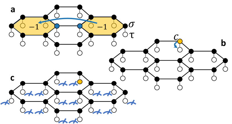
The preparation scheme consists of two steps. In the first step, the system is prepared in the flux-free sector by measuring the flux operators through all plaquettes, and applying unitary operators that correct the fluxes that are detected Dennis et al. (2002). The second step is to prepare the fermionic ground state, whose Chern number is non-zero. The key idea is to introduce auxiliary “bath” degrees of freedom that simulate an effective fermionic bath, coupled to the system’s emergent fermions. Both species of fermions are coupled to the same gauge field, allowing single-fermion hopping between them. We provide an explicit encoding of the system and bath fermions into the physical bosonic qubits, generalizing the one-dimensional construction of Ref. Kishony et al. (2023) to two dimensions. The bath fermions are then used to extract energy and entropy from the system, by performing simulated cyclic adiabatic cooling Matthies et al. (2022); Kishony et al. (2023) followed by measurements of the auxiliary qubits. The steps of the protocol are illustrated in Fig. 1.
Our protocol prepares the ground state of the chiral phase parametrically more efficiently than other methods, such as adiabatic preparation Farhi et al. (2000) or ‘naive’ adiabatic cooling using a simulated bosonic bath Kaplan et al. (2017); Matthies et al. (2022). These methods require a quantum circuit whose depth grows at least polynomially with the system size. In contrast, within our method, the energy density decreases exponentially with the number of cycles performed, and thus the total depth required to achieve a given accuracy in the total ground state energy grows only logarithmically with the system size. In the presence of decoherence, our protocol reaches a steady state whose energy density is proportional to the noise rate, which is parametrically lower than bosonic cooling protocols (where the energy density of the steady state scales as the square root of the noise rate Matthies et al. (2022)).
The protocol presented here can be used to efficiently prepare the ground state of a generic (interacting) fermionic model in 2D. This is done by artificially introducing a gauge field similar to the physical gauge field of the KSL model in order to facilitate the fermionization scheme for the system and the bath. The presence of an effective fermionic bath allows to remove single fermion excitations, while keeping the coupling between the system and auxiliary qubits spatially local.
This paper is organized as follows. In Sec. II we introduce our algorithm for preparing the ground state of the KSL model. In Sec. III we analyze the performance of the protocol both with and without noise via numerical simulations. Finally, in Sec. IV we generalize our protocol for arbitrary interacting fermionic systems.
II Preparing a chiral spin liquid
II.1 Model
In this section we explain how to prepare the ground state of the KSL model in the phase where the emergent fermions carry a non-trivial Chern number, as efficiently as in a topologically trivial phase. The same principle can be applied to arbitrary interacting fermionic Hamiltonians, as we discuss below.
The KSL model consists of spin- degrees of freedom on a honeycomb lattice with strongly anisotropic exchange interactions Kitaev (2006); Winter et al. (2017); Hermanns et al. (2018). The Hamiltonian is written as:
| (1) |
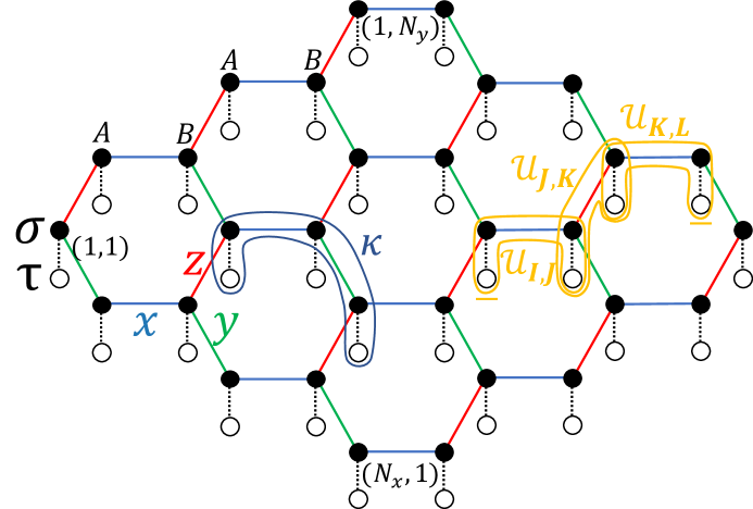
Here, denotes the sites of the honeycomb lattice, where and label the unit cell and labels the two sublattices, and denotes the Pauli matrix at site . The bonds of the lattice are partitioned into three sets – , , and bonds –according to their geometric orientations (see Fig. 2). We denote the corresponding Kitaev anisotropic exchange couplings by and , respectively. The term is a three-spin interaction acting on three neighboring sites denoted by , such that both and are nearest neighbors of site . The term breaks time reversal symmetry, and opens a gap in the bulk that drives the system into the chiral non-Abelian phase Kitaev (2006).
In order to facilitate an efficient protocol to prepare the ground state of (1), we introduce a modified KSL Hamiltonian, , that includes both a system () and a auxiliary () spin at every site of the honeycomb lattice. The auxiliary spins are used to cool the system down to its ground state. The Hamiltonian is illustrated in Fig. 2, and is composed of a sum of two terms:
| (2) |
where is the modified KSL Hamiltonian:
| (3) |
The operators all commute with . Clearly, is identical to in Eq. (1) in the sector . In fact, the two Hamiltonians are related by a unitary transformation for any state of the spins with even parity, . To see this, we note that all of the unitary operators , for , commute with and anticommute individually with and . The transformation from a sector with a given of even parity to the sector {} can be constructed by annihilating pairs of using a product of the unitaries along a path connecting the points . Thus, preparing the ground state of in any known even-parity sector of is equivalent to preparing the ground state of the original KSL Hamiltonian, Eq. (1).
The “control” Hamiltonian , which is used to cool into the ground state of , is chosen as a time-dependent effective Zeeman field acting on with and components and , respectively,
| (4) |
The time dependence of and and the protocol used for cooling are described below.
II.2 Fermionization
It is useful to fermionize the spins and by introducing a set of six Majorana operators per site, subject to the constraint
| (5) |
The spin operators are related to the fermionic ones by:
| (6) |
where and is the totally antisymmetric tensor. This transformation of the spins to fermions is analogous to the one used by Kitaev Kitaev (2006). Note, however, that we have fermionized the and spins together, and as a result, there is a single constraint per site containing both a and a spin. For later use, we note that, using Eqs. (5) and (6), we can write
| (7) |
Using this mapping, we express Hamiltonian (2) as
| (8) |
where we identify the set of conserved gauge fields
| (9) |
The gauge-invariant flux of the gauge field is defined on each hexagonal plaquette that corresponds to the unit cell , as the product of on its edges. In terms of the spin degrees of freedom, this can be written as
| (10) |
The fermionic Hamiltonian (8) with is identical to the Hamiltonian found by fermionizing the original KSL model Kitaev (2006), with playing the role of the “system fermions.” The remaining and operators describe the fermionic modes of the bath, while the operators introduced above Eq. (5) only participate through their roles in setting the values of the conserved gauge fields . The term multiplied by in Eq. (8) allows fermions to hop between the system and the bath, while the term multiplied by acts on the bath fermions alone. Our aim is to prepare the system fermions in the ground state of the Hamiltonian (8) with and no fluxes, i.e., (equivalent to setting , up to a gauge transformation).
II.3 Preparation Protocol
We now present the protocol to prepare the ground state of , starting from an arbitrary initial state. Similarly to Refs. Matthies et al. (2022); Kishony et al. (2023), the protocol consists of cycles which are repeated until convergence to the ground state is achieved. Since the protocol is intended to be implemented on bosonic qubits, in this section we return to the description in terms of the and spins.
In each cycle, the and spins are evolved unitarily for a time period , with a time-dependent Hamiltonian (2) designed to decrease the expectation value of . The unitary evolution is followed by a projective measurement of the spins in the basis. The measurement outcomes are used to determine the Hamiltonian of the next cycle.
In the beginning of the th cycle, the spins are assumed to be in an eigenstate of with known eigenvalues, which we denote by . Before the first cycle, the system is initialized in a state where for all . We then perform the following operations:
- a.
- b.
-
c.
The operators are measured, giving new values . A new cycle then begins from step b.
Importantly, the flux operators commute with . Ideally, they therefore retain their initial values, . In the presence of decoherence on a real quantum simulator, may flip during the cycle. This may require returning to step 1 between cycles, where the flux operators are measured again and unitary operators are applied to correct flipped fluxes, as discussed in Sec. III.2 and Appendix A.
The idea behind this protocol is that, in analogy to adiabatic demagnetization, the coupling between the and spins cools the system towards the ground state of . The spins are initially polarized in a direction parallel to the effective Zeeman fields acting on them. Adiabatically sweeping the Zeeman fields downward while the coupling is non-zero tends to transfer energy into the spins, decreasing the expectation value of . This picture guides the choice of the protocol parameters, , and : should be chosen to be large enough compared to the gap between the ground state and the lowest excited state of , such that sweeping the Zeeman field during the protocol brings the excitations in the system to resonance with the spins. The maximum coupling controls the rate of the cooling. is chosen such that the time evolution is adiabatic with respect to the system’s gap, which sets the maximum allowed values of and : these are chosen such that .
The operation of the cooling protocol is particularly transparent in the fermionic representation, Eq. (8). It is straightforward to check that in the beginning of each cycle, when , the bath fermions and are decoupled from the system fermions, , and are initialized in the ground state of the bath Zeeman Hamiltonian. Sweeping downwards induces level crossings between states of the system () and bath fermions, and when , excitations are transferred from the system to the bath.
II.4 Performance analysis
The fact that the system and bath can be described as emergent fermions which are coupled to the same gauge field means that a single fermionic excitation can be transferred coherently to the bath. This dramatically accelerates the cooling process compared to simpler “bosonic” adiabatic cooling algorithms of the type described in Refs. Boykin et al. (2002); Kaplan et al. (2017); Metcalf et al. (2020); Polla et al. (2021); Zaletel et al. (2021); Rodríguez Pérez (2021); Matthies et al. (2022); Lloyd et al. (2024). In these protocols, only a gauge-neutral pair of fermionic excitations can be transferred from the system to the bath, slowing down the cooling process as the ground state is approached.
Specifically, the performance of our protocol can be understood from simple considerations. The argument mirrors that given in Ref. Kishony et al. (2023) for “gauged cooling” of a one-dimensional quantum Ising model. Since fermionic excitations in the system can independently hop into the bath, each excitation has a finite probability to be removed by the bath in each cycle. The cooling rate is therefore proportional to the energy density of . Approximating the cooling process as a continuous time evolution, we obtain a rate equation for the energy density, :
| (11) |
where is the cooling rate, and is the steady state energy density. The quantities and depend on the protocol parameters, such as , and , and in a realistic noisy quantum simulator, also on the noise rate; in the perfectly adiabatic, noiseless case, , the ground state energy density. Solving Eq. (11), we obtain . In contrast, in a simple adiabatic cooling protocol where only pairs of fermionic excitations can be transferred to the bath, , resulting in a power-law approach to the steady state, .
The fact that the fermionic Hamiltonian (8) is quadratic allows us to analyze the cooling dynamics in a basis in which the excitations are decoupled. Moreover, within the flux-free sector, and assuming that the system is prepared initially such that and hence the signs of the ’s are spatially uniform, the Hamiltonian can be brought into a translationally invariant form by a unitary transformation. This allows an explicit analysis of the performance of the protocol in momentum space, which we present in Appendix C. The analysis verifies the exponential convergence to the steady state with the number of cycles performed, as anticipated above. Moreover, we find that in the ideal (noiseless) case, the steady state energy depends only on the adiabaticity of the protocol with respect to the system’s gap, , whereas the cooling rate depends also on the the adiabaticity with respect to the avoided crossing gaps encountered during the time evolution with . In particular, in the limit where is large compared to , the ground state can be approached with an exponential accuracy.
While these results are demonstrated for the solvable model , which can be mapped to free fermions, we expect them to hold more generally. For example, the performance is not expected to be parametrically affected if quartic interactions between the system fermions are added to Eq. (3). The application of our protocol to general interacting fermionic Hamiltonians is discussed further in Sec. IV.
III Numerical simulations
III.1 Performance without noise
We simulate the fermion cooling algorithm numerically with and without noise using the efficient procedure described in Appendix D which relies on the model being one of free fermions. In all simulations we choose , , in the chiral phase, and use protocol parameters , . Periodic boundary conditions are used unless otherwise stated.
Setting periodic boundary conditions allows us to simulate this translation invariant model in -space point by point. We cool a system of size unit cells in the absence of noise starting from a completely random state. Here, it is assumed that the system has been initialized to the flux-free sector prior to the action of the cooling protocol, which leaves the gauge fields fixed. Time evolution is performed in each momentum sector using an ordinary differential equation solver with a relative tolerance of such that the deviation of the steady state from the ground state is expected to derive predominantly from diabatic transitions.
In the ground state, the Chern number of the fermions is equal to 1. To probe the convergence to the ground state, we define the quantity :
| (12) |
where is the single particle density matrix of either the system () or the bath () fermions. Specifically, , with an analogous expression for . Here, is the Fourier transform of on sublattice with wavevector . In a (pure) Slater determinant state, the quantity becomes the integrated Chern density. We calculate this value by performing a discrete integral in momentum space.
Fig. 4 shows (solid lines) and (dashed lines) at the end of a single cooling cycle before performing the measurement of the spins, as a function of the sweep time, . As the sweep duration is increased, the Chern number of the system approaches and that of the bath approaches , even after a single cycle. The fact that our protocol succeeds in preparing a fermionic chiral ground state starting from a topologically trivial state by a finite depth local unitary circuit is due to the chiral state possessing “invertible” topological order; i.e., stacking two systems with opposite Chern numbers yields a trivial state. Thus, the topological state of the system’s fermions and its inverse (in the bath) can be prepared starting from a trivial state 111Note, however, that overall, the spin system is in a non-invertible topologically ordered state, since the chiral phase of the KSL has fractional (non-Abelian) statistics..
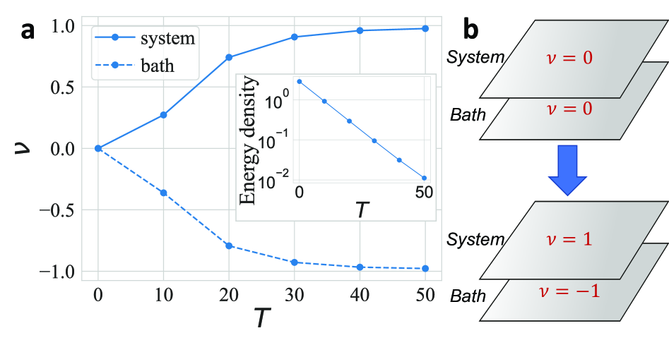
The inset of the Fig. 4 shows the energy density after a single cooling cycle as a function of the duration . As the cycle duration is increased, the system approaches the ground state energy in a single cycle. The deviation from the ground state energy decreases exponentially with increasing .
III.2 Performance with noise
In this section, we numerically test the performance of the proposed cooling algorithm in the presence of noise. For simplicity, the noise is modeled as a uniform depolarizing channel acting on all and qubits at some rate of errors per cooling cycle per qubit. This noise is simulated stochastically as described in Appendix D.
Importantly, the fluxes of the gauge field may be excited by the action of noise on the system. In order to overcome this, one should periodically measure and fix these fluxes, while performing our proposed algorithm for cooling the excitations of the fermions . Fixing the observed fluxes can be done in an analogous way to the action of error correction in the surface code Dennis et al. (2002) by annihilating them in pairs, as explained in Appendix A. When flux excitations are removed (by applying local spin operations), fermionic excitations may be created, and these are then cooled by subsequent cycles of the cooling protocol. Using the protocol, the energy density of the steady state should be proportional to the noise rate, although there is a finite density of flux excitations in the steady state.
We have simulated a KSL system of size unit cells, cooled in the presence of decoherence for multiple cycles. The results are presented in Fig. 5. The energy density is shown at the end of each cycle, with and without the active correction of the flux degrees of freedom. In the simulation with flux correction, the fluxes are measured and removed at the end of each cycle. For simplicity, we have assumed that the measurements are ideal, and the flux correction operations are perfect. In both cases the stochastic action of errors appear as local peaks in the energy density after which the fermionic excitations produced are cooled. However, when errors which excite the flux degrees of freedom occur and these are not corrected, further cycles of fermionic cooling are only able to reach the ground state within the new excited flux sector. After many cycles, a steady state is reached in which the flux degrees of freedom are in a maximally mixed state.
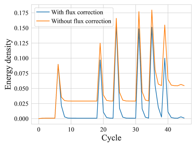
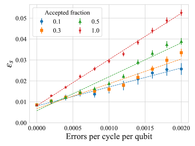
Figure 6 shows the energy density of the steady state reached by cooling a system of size in the presence of noise while correcting the flux degrees of freedom at each cycle. The energy density is linear in the error rate, demonstrating that cooling of both fermionic and flux excitations is done at a rate proportional to their density.
The active correction of the flux degrees of freedom by measurement and feedback provides a natural tool for further error mitigation by post selection. In cycles which require a large weight Pauli correction in order to annihilate the monitored flux excitations, the error together with its correction likely result in the insertion of fermionic excitations which must be removed by further cooling cycles. We denote the weight of the Pauli correction (defined as the number of gates applied to correct the fluxes) at cycle by , and calculate its exponential moving average
| (13) |
where is the exponential cooling rate in the absence of noise. We perform post selection in Fig. 6 by accepting a fraction of the cycles with the smallest values of , using . Performing such post selection succeeds in reducing the expectation value of the energy density. In the limit of a very low accepted fraction of the data, the energy density is reduced approximately by a factor of two at low error rates. In this limit, all cycles in which spins are affected by errors are removed, but cycles in which spins are disturbed remain part of the data. Further post selection can be done by imposing a requirement on the outcomes of the measurements of the degrees of freedom from cycle to cycle Matthies et al. (2022).
IV Extension to arbitrary fermionic Hamiltonians
Our protocol for preparing the ground state of the KSL model can be generalized as a method for preparing the ground state of an arbitrary (interacting) fermionic Hamiltonian in 2D. Given some local target Hamiltonian acting on the system Majorana fermions , we introduce the gauge fields artificially and modify the target Hamiltonian such that the fermions become charged under the gauge field. Namely, we modify each hopping term between site and site in the target Hamiltonian by the product of the gauge fields on a path connecting the two sites. We then introduce the bath fermions , and use Eq. (6) to map the fermionic Hamiltonian (including the hopping between the system and bath fermions, used for cooling the system) onto a bosonic local Hamiltonian acting on the and spins. The ground state of the Hamiltonian is prepared according to the protocol above and this state is related to the ground state of the target Hamiltonian by the known gauge transformation as discussed in Sec. II.
Generalizations to other problems, e.g., with complex spinful fermions or multiple orbitals per site, are straightforward. We also note that Hamiltonians with fermion number conservation can be implemented within our protocol; the fermion number changes during each cycle, but the system is cooled towards the ground state that has a well-defined fermion number set by a chemical potential term.
V Summary
In this work, we have presented an efficient protocol for preparing certain chiral topological states of matter on quantum simulators. Our prime example is the chiral phase of the Kitaev spin model on the honeycomb lattice. Our protocol can be similarly used to prepare invertible topological phases of fermions, such as Chern insulators and chiral topological superconductors. Importantly, our protocol does not require an a-priori knowledge of the ground state wavefunction, and should perform equally well in the presence of interactions (although the phases we prepare have a description in terms of non-interacting fermions). In the absence of interactions and decoherence, the ground state can be reached after a single cycle, up to adiabatic errors (for the non-interacting case, a similar approach was proposed in Ref. Tantivasadakarn et al. (2023)).
Our scheme utilizes a simultaneous fermionization of the target system and the cooling bath with which it is coupled, in order to allow the removal of single fermionic excitations from the system to the bath. Crucially, the protocol relies on repeated measurements of the bath spins that detects the fermionic excitations, and local classical feedback that removes them.
In practice, for running this algorithm on real quantum hardware, one should choose the time duration of the unitary evolution and the number of Trotter steps, , to optimize the trade-off between diabatic errors and Trotterization noise (which decrease upon increasing and ) versus the noise deriving from environmental decoherence and low fidelity gates (which are typically proportional to the number of gates applied, and hence to ). The optimization can be done even without knowledge of the noise characteristics, by minimizing the measured energy of the steady state with respect to the protocol parameters, such as and .
Our protocol offers a parametric advantage compared to other recently-proposed methods to prepare chiral 2D states. Ref. Kalinowski et al. (2023) describes a method to prepare the chiral state of the Kitaev honeycomb model by adiabatic evolution. Due to the gap closing along the path, the excitation energy of the final state (or the ground state fidelity) scales polynomially with the duration of the time evolution. In contrast, in our protocol, no adiabatic path is required, and the excitation energy scales exponentially with the cycle duration. In Ref. Chen et al. (2024), a method for preparing chiral states using sequential quantum circuits is described; this method requires a circuit whose depth scales with the linear size of the system in order to reach a state with a given energy density. Ref. Chu et al. (2023) provides an entanglement renormalization circuit which can prepare chiral states in a depth that scales logarithmically with system size, however this requires the use of long-range unitary gates. By comparison, within our method the required circuit depth is independent of the system size and local qubit connectivity in 2D is sufficient.
We emphasize that, while our method does not require knowing the ground state in advance, the performance of the protocol depends crucially on the topological phase to which the ground state belongs. Developing practical and efficient methods to prepare ground states in more complicated topological phases, such as fractional Chern insulators, is an interesting outstanding challenge.
Acknowledgements.
G.K. and E.B. were supported by CRC 183 of the Deutsche Forschungsgemeinschaft (subproject A01) and a research grant from the Estate of Gerald Alexander. M.R. acknowledges the Brown Investigator Award, a program of the Brown Science Foundation, the University of Washington College of Arts and Sciences, and the Kenneth K. Young Memorial Professorship for support.Appendix A Removing fluxes in 2D
In order to reach the ground state of the 2D KSL, one should prepare the system in a flux-free state of the gauge field and then proceed to cool the fermionic excitations . Fluxes can be removed by measuring the plaquette operators which correspond to local 6-body spin operators shown in Eq. (10). The excitations can be removed in pairs by products of local unitary operations. We note that the operator at a vertex of the honeycomb lattice shared between three hexagons anticommutes with two of the three flux operators on these hexagons, while commuting with the third (as well as all the other plaquettes in the lattice). Therefore, applying such a unitary operator flips the signs of the two corresponding plaquettes, potentially also inserting fermionic excitations. Choosing some pairing of the measured excited plaquettes, one can construct a string of spin operators connecting each pair such that the product anti-commutes only with the plaquette operators at the end points of the string.
Using the above approach, a finite density of flux exitations can be corrected using measurements and feed-forward unitaries (analogously to the error correction protocol in the surface code Dennis et al. (2002)). The composite error (the original error affecting the fluxes together with the correction) is a product of Pauli operators acting on the spins which commutes with all of the flux operators, leaving them unaffected. However, the action of this operator on the system excites a number of residual fermionic excitations proportional to its weight (the number of spins on which it acts). Therefore, assuming a low error rate resulting in a low weight Pauli error with high probability, it is important to construct a correction with a low weight as well by annihilating the flux excitations in local pairs - using a minimum weight perfect matching decoder Edmonds (1965). Otherwise, the density of residual fermionic excitations will scale with system size.
The resulting fermionic excitations left after fusing the fluxes can be removed later by the coupling to the bath. Consequently, in the presence of noise, the combined algorithm (composed of a unitary sweep, measurement of the bath spins and the fluxes, and feed-forward correction of the fluxes) should reach a steady state whose energy density is proportional to the noise rate and is independent of system size. This is the algorithm used in presence of noise, whose results are shown in Figs. 5 and 6.
Appendix B Smooth evolution of time dependent couplings
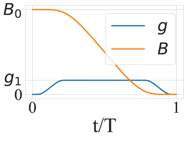
In order to approach the adiabatic limit exponentially with increasing cooling cycle duration , we choose the time dependence of the couplings and to have finite derivatives at all orders. Explicitly, we use a smooth step function as used in Ref. Kishony et al. (2023), defined as
| (14) |
Using this, we express and as
| (15) |
| (16) |
These curves are shown in Fig. 3 for , as chosen in our numerical simulations.
Appendix C Analysis in momentum space
In this section we study the cooling dynamics of the quadratic fermionic Hamiltonian (8) in the flux-free sector with uniform . We choose a gauge where , for which the Hamiltonian is translationally invariant, and Fourier transform the fermionic Hamiltonian to find
| (17) |
where , with the time-dependent Hamiltonian describing the modes at each given by
| (21) |
Here, is a unit matrix, is the submatrix describing the “system” () fermions,
| (22) |
and the matrix that describes hopping between fermionic system and bath () is given by
| (23) |
where we allow the coupling to be sublattice dependent rather than spatially uniform as chosen in the main text. The functions and in Eq. (22) are given by and .
C.1 Adiabatic limit
For the cooling protocol to succeed, it is essential to ensure that for all the off-diagonal terms have a non-zero matrix element between the ground state of the target Hamiltonian, , and the ground state of the Hamiltonian of one of the bath modes, . Importantly, if the system-bath coupling is nonvanishing for all , in the perfectly adiabatic limit the system reaches its ground state after a single cycle (see discussion in Ref. Kishony et al. (2023)). The instantaneous spectrum of in the topological phase with and (where the ground state of the system fermions carries a Chern number of when ) is shown at the point as a function of in Fig. 7. At this point, we find and , such that using only the sublattice bath (taking ) does not allow cooling of fermionic excitations at this point.
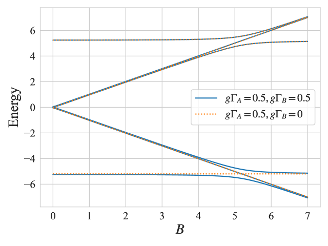
The existence of this gap closing is due to the non-zero Chern number of the target ground state. As varies, the spinor corresponding to the system’s ground state covers the entire Bloch sphere. Therefore, there must be a value of for which the system’s ground state is orthogonal to the spinor formed by acting with the first column of on the bath’s ground states. At this point, the coupling to the bath on the sublattice alone cannot cool the system.
Using two bath sublattices is enough to overcome this problem. As long as matrix is not singular, the spinors obtained by acting with the columns of on the system’s ground state are not identical, and at least one of these spinors has a non-zero overlap with the system’s ground state at each . Note that, in contrast to the topological phase, in the trivial phase where the Chern number vanishes (obtained, e.g., when and ), one bath sublattice would generically be sufficient (with appropriately chosen coupling).
C.2 Diabatic corrections
Deviations from the adiabatic limit have two main effects. First, the protocol does not converge to its steady state after a single cycle, but rather converges to the steady state exponentially with the number of cycles performed. Second, the steady state deviates from the ground state of the system. Importantly, we shall now show that the deviation of the steady state from the ground state due to diabatic errors is controlled by the intrinsic energy gap of the system, and not by the avoided crossing in the middle of the cycle (see Fig. 8). The mid-cycle avoided crossing gap controls the rate of convergence to the steady state.
Returning to the case of , the diabatic corrections are most straightforward to analyze after a series of unitary transformations which map the problem at each into an evolution of three spins. First, we perform a dependent unitary transformation
| (24) |
where is chosen such that , with being the spectrum of the KSL model. This brings the Hamiltonian (21) into a purely antisymmetric form
| (28) |
Next, we write the corresponding vector of complex fermionic annihilation operators in terms of two vectors of Majorana operators: , where with , and similarly for . Using the antisymmetric property of , the many-body Hamiltonian decouples when written in terms of , :
| (29) |
For a given , the parts of the Hamiltonian that depend on and are independent and identical, and it is sufficient to analyze one of them.
C.2.1 Mapping to a three spin problem
The part that depends on can be written in terms of three pseudospin operators, defined such that , , . The basis of the corresponding Hilbert space can be labelled according to the eigenvalues of ; we denote the basis states as . The -dependent part of the Hamiltonian is written as
| (30) |
We have thus mapped the problem into that of three coupled spins. The Hamiltonian of the sector has the same form, and can be treated similarly. Note that the spins are distinct from the physical ones, and .
C.2.2 Solution of the three spin problem
At the Hamiltonian is diagonalized in the orthonormal basis , , , with energies given by , , , . At finite , the first two states remain decoupled. The Hamiltonian in the complementary subspace written in this basis is given by
| (31) |
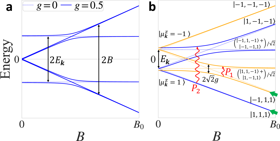
and its spectrum is shown as a function of for (solid lines) and for (dotted lines) in Fig. 8b. Turning on a non-zero couples to and . (Note that : the even and odd parity sectors of total pseudospin are decoupled.)
Each cooling cycle is initialized with the bath spins , in their respective ground states, i.e., the system is initialized in some mixture of the states . For , the energies of the eigenstates and cross at , while the state remains spectrally separated from the only state it is directly coupled to, . With a finite , the crossing becomes an avoided crossing and in the adiabatic limit, the states and are exchanged under the time evolution, while evolves trivially.
Away from the adiabatic limit, we denote the diabatic transition probability for the , pair as and the diabatic transition probability between and as (see Fig. 8b). For and assuming is constant for times where , is approximately given by the Landau-Zener formula, for some constant . The second transition probability, , is determined by the single particle gap of the target Hamiltonian, , where is the minimal gap. We neglect the possibility for transitions to the states as a second order effect, occurring with probability of the order of .
C.2.3 Analysis of the cooling dynamics
A single cycle of the cooling protocol, including the measurement of the ancilla spins, can be described as a map from the initial density matrix for the system (corresponding to the pseudospin ) to the final one, i.e., the dynamics realize a quantum channel. The protocol consists of applying this quantum channel to the system multiple times, until a steady state is reached.
We number the four states participating in the dynamics , , , by for brevity and denote the corresponding density matrix by
| (32) |
The final step of the protocol, in which are measured and the signs of are adjusted accordingly for the next cycle, is equivalent to a resetting operation taking after the measurement. The action of this operation on the density matrix is given by
| (33) |
The unitary time evolution step acts as
where
| (34) |
where and are the transition probabilities between the different states (see Sec. C.2.2 and Fig. 8b), and we denote the complementary probabilities to by . Finally, under the full protocol cycle consisting of unitary evolution followed by measurement and reset,
| (35) |
where
| (36) |
Here, the complex phases cancel. If we take , then the steady state of the protocol is the desired ground state () since there is no probability for any transition. In general, the steady state of these dynamics is given by
| (37) |
the steady state is a mixture of the ground state () and the excited state (). The probability to be in the ground state is given by
| (38) |
We denote the eigenvalues of the quantum channel by (where corresponds to the steady state). The eigenvalues, , , and determine the rate in cycles at which the steady state is exponentially approached. These are given by
| (39) |
| (40) |
| (41) |
The largest among these (i.e., the eigenvalue closest to 1) is , and hence this eigenvalue controls the approach to the steady state: asymptotically, the deviation from the steady state scales with the number of cycles as , where 222Note that, in general, . In the special case , and the steady state becomes degenerate. For any other value of , the system converges to the steady state..
Interestingly, Eq. (38) shows that for , the steady state is exactly the ground state, independent of the value of . This is due to the fact that, for , there is no way to escape from the ground state once it is reached. However, the rate of approach to the ground state does depend on .
Appendix D Single-particle density matrix simulation of free fermions
The free evolution of a quantum many-body system under a quadratic fermionic Hamiltonian, including measurements and resets of single sites and Pauli errors, can be traced numerically efficiently, requiring only time and memory that scale as polynomials of the system size. Here, we briefly describe the technique used to simulate the noisy dynamics of the cooling process discussed in Sec. III.2. The technique is the same as that used in Ref. Kishony et al. (2023).
We keep track of the single particle density matrix as well as the values of the gauge field as they evolve under the noisy cooling dynamics. This allows us to calculate any quadratic observables, and the energy in particular.
During free evolution under the Hamiltonian (8) of the main text within a fixed sector of the gauge field , the single particle density matrix evolves under a unitary matrix by conjugation, . This unitary is given by the time ordered exponentiation of the Hamiltonian in matrix form, and can be found numerically by Trotterization or using an ordinary differential equation solver. In Sec. III.2 we use second order Trotterization, making steps per cooling cycle. Importantly, the unitary depends on the values of the gauge field which are looked up for its computation.
The resetting operation of the bath fermions at the end of each cycle is handled as in Ref. Kishony et al. (2023). This amounts to setting all matrix elements of in the two rows and the two columns corresponding to and to to zero, and then setting the block at their intersection to the values found at .
Depolarizing noise is implemented through stochastic application of Pauli errors before each Trotter step of the time evolution and for each spin () with probability of . The Pauli operators are bilinear in the fermions (6), such that they correspond to evolution under a quadratic fermionic Hamiltonian. Pauli errors act on the Majorana fermions, flipping the signs of two of the three gauge fields incident to site .
Measuring the flux degrees of freedom within this framework simply requires reading off the product of the values of the gauge fields around the corresponding plaquettes. These values are well defined at every point in time for each trajectory in these simulations, and their fluctuations can be obtained by averaging over multiple trajectories with stochastic noise. Correcting these fluxes in order to return to the flux-free sector, as described in Appendix A, is done by applying a unitary correction given by a product of Pauli operators.
References
- Cirac and Zoller (2012) J. Ignacio Cirac and Peter Zoller, “Goals and opportunities in quantum simulation,” Nature Physics 8, 264–266 (2012).
- Georgescu et al. (2014) I. M. Georgescu, S. Ashhab, and Franco Nori, “Quantum simulation,” Reviews of Modern Physics 86, 153–185 (2014).
- Chen et al. (2010) Xie Chen, Zheng-Cheng Gu, and Xiao-Gang Wen, “Local unitary transformation, long-range quantum entanglement, wave function renormalization, and topological order,” Phys. Rev. B 82, 155138 (2010).
- McClean et al. (2016) Jarrod R McClean, Jonathan Romero, Ryan Babbush, and Alán Aspuru-Guzik, “The theory of variational hybrid quantum-classical algorithms,” New Journal of Physics 18, 023023 (2016).
- Moll et al. (2018) Nikolaj Moll, Panagiotis Barkoutsos, Lev S Bishop, Jerry M Chow, Andrew Cross, Daniel J Egger, Stefan Filipp, Andreas Fuhrer, Jay M Gambetta, Marc Ganzhorn, Abhinav Kandala, Antonio Mezzacapo, Peter Müller, Walter Riess, Gian Salis, John Smolin, Ivano Tavernelli, and Kristan Temme, “Quantum optimization using variational algorithms on near-term quantum devices,” Quantum Science and Technology 3, 030503 (2018).
- Tilly et al. (2022) Jules Tilly, Hongxiang Chen, Shuxiang Cao, Dario Picozzi, Kanav Setia, Ying Li, Edward Grant, Leonard Wossnig, Ivan Rungger, George H. Booth, and Jonathan Tennyson, “The variational quantum eigensolver: A review of methods and best practices,” Physics Reports 986, 1–128 (2022).
- Farhi et al. (2000) Edward Farhi, Jeffrey Goldstone, Sam Gutmann, and Michael Sipser, “Quantum computation by adiabatic evolution,” (2000), arXiv:quant-ph/0001106 [quant-ph] .
- Childs et al. (2001) Andrew M. Childs, Edward Farhi, and John Preskill, “Robustness of adiabatic quantum computation,” Phys. Rev. A 65, 012322 (2001).
- Alan Aspuru-Guzik and Anthony D. Dutoi and Peter J. Love and Martin Head-Gordon (2005) Alan Aspuru-Guzik and Anthony D. Dutoi and Peter J. Love and Martin Head-Gordon, “Simulated quantum computation of molecular energies,” Science 309, 1704–1707 (2005).
- Albash and Lidar (2018) Tameem Albash and Daniel A. Lidar, “Adiabatic quantum computation,” Rev. Mod. Phys. 90, 015002 (2018).
- Motta et al. (2019) Mario Motta, Chong Sun, Adrian T. K. Tan, Matthew J. O’Rourke, Erika Ye, Austin J. Minnich, Fernando G. S. L. Brandão, and Garnet Kin-Lic Chan, “Determining eigenstates and thermal states on a quantum computer using quantum imaginary time evolution,” Nature Physics 16, 205–210 (2019).
- Lin et al. (2021) Sheng-Hsuan Lin, Rohit Dilip, Andrew G. Green, Adam Smith, and Frank Pollmann, “Real- and imaginary-time evolution with compressed quantum circuits,” PRX Quantum 2, 010342 (2021).
- Jouzdani et al. (2022) Pejman Jouzdani, Calvin W. Johnson, Eduardo R. Mucciolo, and Ionel Stetcu, “Alternative approach to quantum imaginary time evolution,” Phys. Rev. A 106, 062435 (2022).
- Boykin et al. (2002) P. Oscar Boykin, Tal Mor, Vwani Roychowdhury, Farrokh Vatan, and Rutger Vrijen, “Algorithmic cooling and scalable NMR quantum computers,” Proceedings of the National Academy of Sciences 99, 3388–3393 (2002).
- Kaplan et al. (2017) David B. Kaplan, Natalie Klco, and Alessandro Roggero, “Ground states via spectral combing on a quantum computer,” (2017), arXiv:1709.08250 [quant-ph] .
- Metcalf et al. (2020) Mekena Metcalf, Jonathan E. Moussa, Wibe A. de Jong, and Mohan Sarovar, “Engineered thermalization and cooling of quantum many-body systems,” Phys. Rev. Res. 2, 023214 (2020).
- Polla et al. (2021) Stefano Polla, Yaroslav Herasymenko, and Thomas E. O’Brien, “Quantum digital cooling,” Phys. Rev. A 104, 012414 (2021).
- Zaletel et al. (2021) Michael P. Zaletel, Adam Kaufman, Dan M. Stamper-Kurn, and Norman Y. Yao, “Preparation of low entropy correlated many-body states via conformal cooling quenches,” Phys. Rev. Lett. 126, 103401 (2021).
- Rodríguez Pérez (2021) David Rodríguez Pérez, “Quantum error mitigation and autonomous correction using dissipative engineering and coupling techniques,” Ph.D. thesis, Colorado School of Mines (2021).
- Matthies et al. (2022) Anne Matthies, Mark Rudner, Achim Rosch, and Erez Berg, “Programmable adiabatic demagnetization for systems with trivial and topological excitations,” (2022).
- Lloyd et al. (2024) Jerome Lloyd, Alexios Michailidis, Xiao Mi, Vadim Smelyanskiy, and Dmitry A. Abanin, “Quasiparticle cooling algorithms for quantum many-body state preparation,” (2024), arXiv:2404.12175 [quant-ph] .
- Piroli et al. (2021) Lorenzo Piroli, Georgios Styliaris, and J. Ignacio Cirac, “Quantum circuits assisted by local operations and classical communication: Transformations and phases of matter,” Phys. Rev. Lett. 127, 220503 (2021).
- Tantivasadakarn et al. (2023) Nathanan Tantivasadakarn, Ashvin Vishwanath, and Ruben Verresen, “Hierarchy of topological order from finite-depth unitaries, measurement, and feedforward,” PRX Quantum 4, 020339 (2023).
- Kitaev (2003) Alexei Kitaev, “Fault-tolerant quantum computation by anyons,” Annals of Physics 303, 2–30 (2003), arXiv:quant-ph/9707021 [quant-ph] .
- Kitaev (2006) Alexei Kitaev, “Anyons in an exactly solved model and beyond,” Annals of Physics 321, 2–111 (2006).
- Dennis et al. (2002) Eric Dennis, Alexei Kitaev, Andrew Landahl, and John Preskill, “Topological quantum memory,” Journal of Mathematical Physics 43, 4452–4505 (2002).
- Kishony et al. (2023) Gilad Kishony, Mark S. Rudner, Achim Rosch, and Erez Berg, “Gauged cooling of topological excitations and emergent fermions on quantum simulators,” (2023), arXiv:2310.16082 [cond-mat.str-el] .
- Winter et al. (2017) Stephen M Winter, Alexander A Tsirlin, Maria Daghofer, Jeroen van den Brink, Yogesh Singh, Philipp Gegenwart, and Roser Valentí, “Models and materials for generalized kitaev magnetism,” Journal of Physics: Condensed Matter 29, 493002 (2017).
- Hermanns et al. (2018) Maria Hermanns, Itamar Kimchi, and Johannes Knolle, “Physics of the kitaev model: Fractionalization, dynamic correlations, and material connections,” Annual Review of Condensed Matter Physics 9, 17–33 (2018).
- Kalinowski et al. (2023) Marcin Kalinowski, Nishad Maskara, and Mikhail D. Lukin, “Non-abelian floquet spin liquids in a digital rydberg simulator,” Physical Review X 13 (2023), 10.1103/physrevx.13.031008.
- Note (1) Note, however, that overall, the spin system is in a non-invertible topologically ordered state, since the chiral phase of the KSL has fractional (non-Abelian) statistics.
- Chen et al. (2024) Xie Chen, Michael Hermele, and David T. Stephen, “Sequential adiabatic generation of chiral topological states,” (2024), arXiv:2402.03433 [cond-mat.str-el] .
- Chu et al. (2023) Su-Kuan Chu, Guanyu Zhu, and Alexey V. Gorshkov, “Entanglement renormalization circuits for chiral topological order,” (2023), arXiv:2304.13748 [quant-ph] .
- Edmonds (1965) Jack Edmonds, “Paths, trees, and flowers,” Canadian Journal of Mathematics 17, 449–467 (1965).
- Note (2) Note that, in general, . In the special case , and the steady state becomes degenerate. For any other value of , the system converges to the steady state.