Logarithmic regret in the ergodic Avellaneda–Stoikov market making model

Jialun Cao1 Galen.Cao@ed.ac.uk David Šiška1 D.Siska@ed.ac.uk Lukasz Szpruch1,2 L.Szpruch@ed.ac.uk  and  Tanut Treetanthiploet3 tanut.t@infinitaskt.com 1School of Mathematics, University of Edinburgh, United Kingdom 2The Alan Turing Institute, London, United Kingdom 3Infinitas by Krungthai, Bangkok, Thailand
Abstract.

We analyse the regret arising from learning the price sensitivity parameter $\kappa$ of liquidity takers in the ergodic version of the Avellaneda–Stoikov market making model. We show that a learning algorithm based on a regularised maximum-likelihood estimator for the parameter achieves the regret upper bound of order $\ln^{2}T$ in expectation. To obtain the result we need two key ingredients. The first are tight upper bounds on the derivative of the ergodic constant in the Hamilton–Jacobi–Bellman (HJB) equation with respect to $\kappa$. The second is the learning rate of the maximum-likelihood estimator which is obtained from concentration inequalities for Bernoulli signals. Numerical experiment confirms the convergence and the robustness of the proposed algorithm.

Key words and phrases:
Regret, Online learning, Adaptive control, Ergodic control, Market making, Maximum likelihood estimation
2020 Mathematics Subject Classification:
Primary 93E35; Secondary 93C40, 93C41, 93E20, 91G80

1. Introduction

Market makers are market participants who are willing to both buy and sell an asset at any time thus providing liquidity. They aim to make a profit from the spread, i.e. buying at a lower price (bid) and selling at a higher price (ask) at the cost of carrying inventory risk. While the principle is simple, executing this consistently profitably is not straightforward due to price volatility, various market micro-structure considerations, information asymmetry and other factors.

Avellaneda and Stoikov [9] have proposed a formulation of the market making task as a stochastic control problem within a parsimonious model. Since then, the framework has been extensively studied and extended to incorporate various additional features, see [26, 34, 15, 14, 12, 13] and the references therein.

In this paper we introduce the ergodic formulation of the model. We will establish an upper bound on regret of order $\ln^{2}T$ arising from having to learn the key unknown parameter online (while executing a strategy) in the ergodic market making model. In the remainder of the introduction we will briefly introduce the ergodic market making model, the concept of regret, provide a literature review and highlight the main contributions of this paper. In Section 2 we will state all the assumptions and results in detail.

Ergodic formulation of the Avellaneda–Stoikov model

The market maker places one buy / sell order at distances $\delta^{-}$, $\delta^{+}$ from the mid price denoted $S_{t}$ and updates these continuously as new information arrives. These are the controls. On average $\lambda^{\pm}$ per unit of time buy / sell market orders (orders from liquidity takers) arrive. These hit the limit order posted by the market maker with probability of $e^{-\kappa\delta^{\pm}}$. The system thus has the controlled dynamics given by

$$\begin{split}dS_{t}&=\sigma dW_{t},\quad S_{0}=s_{0}\,,\\ dQ_{t}^{\delta^{\pm}}&=dN_{t}^{\delta,-}-dN_{t}^{\delta,+},\quad Q_{0}=q_{0}\,,\\ dX^{\delta^{\pm}}_{t}&=(S_{t-}+\delta_{t}^{+})dN_{t}^{\delta,+}-(S_{t-}-\delta_{t}^{-})dN_{t}^{\delta,-},\quad X_{0}=x_{0}\,,\end{split}$$

where $(S_{t})_{t\geq 0}$ is the exogenous mid-price process, $(Q_{t}^{\delta^{\pm}})_{t\geq 0}$ is the market maker’s inventory and $(X^{\delta^{\pm}}_{t})_{t\geq 0}$ is the market maker’s cash balance. The inventory and cash processes are driven by $N_{t}^{\delta,\pm}$, two independent Poisson jump processes with intensities $\lambda^{\pm}e^{-\kappa\delta^{\pm}}$. The market maker wishes to maximize the long-run average reward which sums the earnings and changes to mark-to-market value of their holdings of the risky asset but is subject to a quadratic inventory penalty expressing their risk aversion:

$$J(q,x,S;\delta^{\pm})=\lim_{T\rightarrow+\infty}\frac{1}{T}\mathbb{E}_{q,x,S}\bigg{[}\int_{0}^{T}\mathrm{d}(X^{\delta^{\pm}}_{t}+S_{t}Q_{t}^{\delta^{\pm}})-\phi\int_{0}^{T}(Q^{\delta^{\pm}}_{t})^{2}\,\mathrm{d}t\bigg{]}\,.$$

If the values of all the parameters are known then the market maker can solve the ergodic Hamilton–Jacobi–Bellman (HJB) equation associated to the problem and obtain the optimal strategy in closed form as we show in Section 2.1. Under the optimal strategy, the market maker’s reward, per of unit time, will be given by the ergodic constant

$$\gamma(\kappa)=\sup_{\delta^{\pm}}J(x,S,q;\delta^{\pm}).$$

Online learning and regret

The model parameters are: liquidity takers orders’ arrival rates $\lambda^{\pm}$, the price sensitivity of the liquidity takers $\kappa$, the mid price volatility $\sigma$ (which actually plays no role as the mid price process is a martingale) and the risk aversion $\phi$. The market maker chooses their risk aversion and thus it’s not a parameter that they would need to learn. The liquidity takers orders’ arrival rates $\lambda^{\pm}$ can be observed and learned offline (without participating in the market) since, in the framework of the model where our market maker is assumed to provide a relatively small fraction of the overall liquidity, it is unlikely that the presence of their volume in the market would impact the rate of liquidity taking. This leaves $\kappa$ and this is the key parameter. It is not reasonable to assume that this could be learned offline. Exchanges provide visibility of the order book and some information on executed trades but often not enough to allow good offline estimate for $\kappa$. Furthermore other market makers will react to the presence of the additional volume placed by our market maker at the distance $\delta^{\pm}$ thus potentially rendering any offline estimate of $\kappa$ invalid. Indeed, some may choose to place their volume at better price (they want to trade) than the spread given by our market maker while others may wish to place the volume at worse price (they may think our market maker knows something about the price they don’t).

The key parameter to learn online (i.e. while participating in the market) is thus $\kappa$. At each time $t\geq 0$ the market maker will have their estimate of the parameter denoted $\kappa_{t}$ while the true, unknown, value is $\kappa^{\ast}$. They can solve the ergodic control problem and obtain the strategy which would be optimal if $\kappa_{t}$ would be the true parameter. Let us denote this by strategy by $\psi^{\kappa_{t},\pm}$.

Our aim is to gain asymptotic understanding of the regret given by

(1) $$\mathcal{R}(T)=\gamma(\kappa^{\star})T-\mathbb{E}_{q,x,S}\bigg{[}\int_{0}^{T}\mathrm{d}\big{(}X^{\psi^{\kappa_{t},\pm}}_{t}+S_{t}Q^{\psi^{\kappa_{t},\pm}}_{t}\big{)}-\phi\int_{0}^{T}(Q^{\psi^{\kappa_{t},\pm}}_{t})^{2}\,\mathrm{d}t\bigg{]}\,.$$

This is the difference between the optimal, inaccessible, reward up to time $T$ and the reward the agent gains by following their chosen method of learning.

If the market maker would use a fixed $\kappa\neq\kappa^{\ast}$ then their expected regret would be roughly $(\gamma(\kappa^{\ast})-\gamma(\kappa))T$ i.e. linear. Any algorithm which achieves sub-linear regret is learning. We construct a regularised maximum-likelihood estimator, see (25), and employ it in Algorithm 1, to achieve the expected regret upper bound of order $\ln^{2}T$. See Theorem 19.

Existing literature

Before we proceed to discussing online learning let us mention the “offline” learning approach in Cartea [12]. There, parameter uncertainty for the finite-time-horizon market making model is accepted and robust controls which take model ambiguity into account are derived.

Online learning and regret analysis in stochastic control has been studied in the context of adaptive control and reinforcement learning. Broadly, there are three relatively distinct areas.

The first area is discrete and finite space and time Markov decision problems (either discounted or ergodic). Here regret of order $\sqrt{T}$ is expected in the general setting and with additional structural assumptions regret of order $\ln T$ is achievable, see Auer and Ortner [8], Auer et al. [7] and references therein.

The second area is still discrete time with linear dynamics and convex cost / concave rewards. This makes the setting tractable even in the case of more general state spaces and action spaces. This is the setting most explored in the literature over the years: Kumar [33], Campi and Kumar [11], Abbasi-Yadkori [1], Abeille and Lazaric [2], Agarwal et al. [4] Dean et al. [19], Cohen et al. [18], Cassel et al. [17], Faradonbeh et al. [22], Lale et al. [35], Simchowitz and Foster [37], Hambly et al. [29] and undoubtedly some others. The theme is again that order $\sqrt{T}$ is achievable and if more can be assumed (e.g. “identifiability conditions” which imply “self-exploration”) then regret upper bound of order $\ln T$ holds.

Finally, the third which is the continuous-time, in linear-convex framework setting is the least explored. Guo et al. [28] considers finite-time-horizon linear-convex episodic learning and propose algorithm which achieves order $\sqrt{N\ln N}$ regret (with $N$ being the episode number) under an identifiability assumption. In Basei et al. [10] where, the episodic learning LQR is studied, regret bound of order $(\ln N)(\ln(\ln N))$ is obtained, again under an identifiability assumption. Szpruch et al. [39] show that without the identifiability assumption it is possible to balance exploration and exploitation (by adding an entropic regularizer) to achieve order $\sqrt{N}$ regret. In Szpruch et al. [38] this is improved to $\ln^{2}N$ by means of establishing stronger (2nd order) regularity result for the dependence of the problem value function on the unknown system parameters.

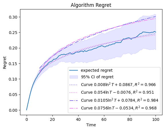
Having reviewed existing results, we note that the study of regret in continuous-time ergodic control has been limited. Fruit and Lazaric [23] derive regret bounds in semi-Markov decision processes (SMDP) within the ergodic setting and show that the regret of order $\sqrt{T}$ is achievable under certain assumptions (e.g. lump sum reward). In Gao and Zhou [24], the order of regret is improved to $\ln T$ by focusing on continuous-time Markov decision processes, a more specific case than SMDP. This represents a significant step forward, showing that logarithmic regret is achievable in continuous-time ergodic frameworks. Nevertheless jump diffusion dynamics and non-linear running rewards required in the Avellaneda–Stoikov model do not fit into the framework of any of the existing papers. From other results in the literature we see that our result showing $\ln^{2}T$ regret is nearly as good as it gets but a question remains whether this is optimal i.e. what is the regret lower bound in this setting. The numerical experiment shows regret of order $\ln^{2}T$ is a good fit for what we observe, see Figure 3.

Our contributions

To the best of authors’ knowledge this is the first paper on regret analysis for ergodic control of jump diffusions. The control problem we focus on is the ergodic version of the Avellaneda–Stoikov market making model and we show that the expected regret has an upper bound of order of $\ln^{2}T$.

There are three main ingredients which allow us to obtain this result. First, we prove existence of and convergence to an invariant measure in the ergodic Avellaneda–Stoikov market making model. While the well-posedness of the ergodic problem follows mostly from the analysis carried out in Guéant and Manziuk [27] the result on existence of and convergence to the invariant measure is new and relies on newly established explicit solution the the ergodic HJB corresponding to our problem.

Second, we obtain bounds on the second derivative of the average earnings per unit time (the ergodic constant) with respect to the parameter $\kappa$ which has to be learned.

Finally, using concentration inequalities for Bernoulli random variables we show that a regularised maximum likelihood estimator yields a high probability bound of order $N^{-1/2}$ on the distance between the true value $\kappa^{\ast}$ and the estimate $\kappa_{N}$ obtained after $N$ market orders have arrived.

2. Main results

In this section, we will introduce the ergodic Avellaneda–Stoikov market making model and state the main results of the paper.

The market maker (agent) proposes bid$(-)$ and ask$(+)$ depths (control) $(\delta^{\pm}_{t})_{t\geq 0}$ pegged to the mid-price of an asset and wish to make profit from the spread. The space $(\Omega^{W},\mathcal{F}^{W},\mathbb{P}^{W})$ supports a Brownian motion $(W_{t})_{t\geq 0}$ that describes the asset mid-price process $(S_{t})_{t\geq 0}$, following the dynamics

(2) $$dS_{t}=\sigma dW_{t},\quad S_{0}=s_{0}\,.$$

Apart from the market maker, there are liquidity takers sending market orders (MOs) at random times. The model assumes that the arrivals of buy$(+)$ and sell$(-)$ MOs, $(M_{t}^{\pm})_{t\geq 0}$, follow two independent Poisson processes with intensities $\lambda^{+}$ and $\lambda^{-}$ defined on $(\Omega^{M},\mathcal{F}^{M},\mathbb{P}^{M})$. Given two independent IID sequences $U^{\pm}_{i}\sim U(0,1)$ defined on $(\Omega^{U},\mathcal{F}^{U},\mathbb{P}^{U})$ an incoming market buy/sell order trades with the sell/buy volume posted by the market maker when $U^{\pm}_{M^{\pm}_{t}}\geq e^{-\kappa^{\pm}\delta_{t}^{\pm}}$. The probability space for the model is thus

(3) $$\begin{split}(\Omega,\mathcal{F},\mathbb{P})=\big{(}\Omega^{W}\times\Omega^{M}\times\Omega^{U},\mathcal{F}^{W}\otimes\mathcal{F}^{M}\otimes\mathcal{F}^{U},\mathbb{P}^{W}\otimes\mathbb{P}^{M}\otimes\mathbb{P}^{U}\big{)}\,.\end{split}$$

The filtration is $\mathbb{F}:=(\mathcal{F}_{t})_{t\geq 0}$, where $\mathcal{F}_{t}=\sigma(W_{r},r\leq t)\vee\sigma(M_{r}^{\pm},r\leq t)\vee\sigma(U^{+}_{M^{+}_{r}},r\leq t)\vee\sigma(U^{-}_{M^{-}_{r}},r\leq t)$. Let $\underline{q}\in\mathbb{Z}^{-}$ and $\bar{q}\in\mathbb{Z}^{+}$ denote the market maker’s inventory limits. The market maker will stop posting buy/sell orders when their inventory is at $\bar{q}$ and at $\underline{q}$ respectively. At other times their strategy is to post at a distance $\delta^{\pm}\in\mathbb{R}$ from the mid-price $S_{t}$. Clearly, the strategy $\delta^{\pm}$ must be adapted to the filtration $\mathbb{F}$. Let $(N_{t}^{\delta,\pm})_{t\geq 0}$ be the controlled counting processes for the agent’s filled buy/sell orders, i.e.

$$N_{t}^{\delta,\pm}=N_{t-}^{\delta,\pm}+(M^{\pm}_{t}-M^{\pm}_{t-})\bm{1}_{\left\{U^{\pm}_{M^{\pm}_{t}}\geq e^{-\kappa^{\pm}\delta_{t-}^{\pm}}\right\}}\,.$$

Hence the inventory process $(Q_{t})_{t\geq 0}$ of the market maker is

(4) $$dQ_{t}^{\delta^{\pm}}=dN_{t}^{\delta,-}-dN_{t}^{\delta,+},\quad Q_{0}=q_{0}\,\text{ and }\,\underline{q}\leq Q_{t}\leq\bar{q}\,.$$

Let us write $\Omega^{Q}=[\underline{q},\bar{q}]\cap\mathbb{Z}$, so that $Q_{t}$ takes values in $\Omega^{Q}$ for $t\geq 0$. Let $(X_{t})_{t\geq 0}$ denote the market maker’s cash balance, satisfying

(5) $$dX^{\delta^{\pm}}_{t}=(S_{t-}+\delta_{t}^{+})dN_{t}^{\delta,+}-(S_{t-}-\delta_{t}^{-})dN_{t}^{\delta,-},\quad X_{0}=x_{0}\,.$$

Let us define the class of admissible policies as

(6) $$\begin{split}\mathcal{A}=\big{\{}(\delta^{\pm}_{t})_{t\geq 0}&:\text{$\overline{\mathbb{R}}$-valued, bounded from below, progressively measurable }\\ &\text{w.r.t. $\mathbb{F}$ and s.t. for any $T>0$ we have }\mathbb{E}\int_{0}^{T}|\delta^{\pm}_{t}|^{2}\,\mathrm{d}t<\infty\big{\}}\,.\end{split}$$

2.1. The ergodic market making model

In this section we will formulate the ergodic control problem, state key results connecting the control formulation with the ergodic HJB equation, provide explicit solution for the ergodic HJB and formulae for the Markovian ergodic optimal controls, state equilibrium properties of the system and state a result on convergence to equilibrium.

Control problem formulation

The market maker aims to maximise a long-run average reward of the accumulated PnL with a running inventory penalty. Let $J(x,S,q;\delta^{\pm})$ be the ergodic reward functional given by

(7) $$J(q,x,S;\delta^{\pm})=\lim_{T\rightarrow+\infty}\frac{1}{T}\mathbb{E}_{q,x,S}\bigg{[}\int_{0}^{T}\mathrm{d}(X^{\delta^{\pm}}_{t}+S_{t}Q_{t}^{\delta^{\pm}})-\phi\int_{0}^{T}(Q^{\delta^{\pm}}_{t})^{2}\,\mathrm{d}t\bigg{]}\,,$$

where the notation $\mathbb{E}_{q,x,S}[\cdot]$ represents expectation conditional on $Q_{0}=q,X_{0}=x,S_{0}=S$ and $\phi\geq 0$ is the running inventory penalty parameter. For the optimal ergodic control problem, the purpose is to give a characterisation of the optimal long-run average reward, also known as the ergodic constant

$$\gamma=\sup\Big{\{}J(q,x,S;\delta^{\pm}):\delta^{\pm}\in\mathcal{A}\Big{\}}\,,$$

and to construct an optimal feedback (Markov) control $\psi^{\pm}$. We will later see that $\gamma$ is indeed independent of $q,x,S$ and thus calling it the ergodic constant is justified. Of course it still depends on all the model parameters, in particular on $\kappa$.

Let us define a running reward function $f:\Omega^{Q}\times\overline{\mathbb{R}}^{2}\rightarrow\mathbb{R}$ as

(8) $$f(q;\delta^{\pm})=\delta^{+}\lambda^{+}e^{-\kappa^{+}\delta^{+}}+\delta^{-}\lambda^{-}e^{-\kappa^{-}\delta^{-}}-\phi q^{2}\,.$$

By (2), (4) and (5), we have

$$\begin{split}&d(X^{\delta^{\pm}}_{t}+S_{t}Q^{\delta^{\pm}}_{t})=dX^{\delta^{\pm}}_{t}+S_{t}dQ^{\delta^{\pm}}_{t}+Q^{\delta^{\pm}}_{t}dS_{t}+dS_{t}dQ^{\delta^{\pm}}_{t}\\ &=(\delta^{+}\lambda^{+}e^{-\kappa^{+}\delta^{+}}+\delta^{-}\lambda^{-}e^{-\kappa^{-}\delta^{-}})dt+\delta^{+}d\tilde{N}_{t}^{\delta,+}+\delta^{-}d\tilde{N}_{t}^{\delta,-}+\sigma Q^{\delta^{\pm}}_{t}dW_{t}\,,\end{split}$$

where $\tilde{N}_{t}^{\delta,\pm}$ are independent compensated Poisson processes. As the intensities of $N_{t}^{\delta^{+}}$ and $N_{t}^{\delta^{-}}$ would be 00 whenever $\delta^{+}=+\,\infty$ and $\delta^{-}=+\,\infty$ and otherwise $\delta^{\pm}\in\mathcal{A}$ is clearly square integrable, therefore $\mathbb{E}\big{[}\int_{0}^{T}\delta^{+}d\tilde{N}_{t}^{\delta,+}\big{]}=0$ and $\mathbb{E}\big{[}\int_{0}^{T}\delta^{-}d\tilde{N}_{t}^{\delta,-}\big{]}=0$. Moreover, $(Q_{t}^{\delta^{\pm}})_{t\geq 0}\in\Omega^{Q}$ is $\mathcal{F}_{t}-$adapted and bounded and so $\mathbb{E}\big{[}\int_{0}^{T}\sigma Q^{\delta^{\pm}}_{t}dW_{t}\big{]}=0$. Hence the ergodic market making control problem can be reduced from dimension of 3 to 1 by Fubini’s theorem

(9) $$J(q;\delta^{\pm})=\lim_{T\rightarrow+\infty}\frac{1}{T}\mathbb{E}_{q}\Big{[}\int_{0}^{T}f(Q^{\delta^{\pm}}_{t};\delta^{\pm})\,\mathrm{d}t\Big{]}\,,\quad\gamma=\sup\Big{\{}J(q;\delta^{\pm}):\delta^{\pm}\in\mathcal{A}\Big{\}}\,.$$

To analyse the ergodic control problem (9), some preliminaries are required. We start with the existence and uniqueness analysis for the classical market making problem in the discounted finite and infinite-time-horizon settings.

Key results for the discounted finite time and infinite-time problems

We first define the unoptimised Hamiltonian function $H:\Omega^{Q}\times\mathbb{R}^{2}\times\mathbb{R}^{2}\rightarrow\mathbb{R}$ and the optimised Hamiltonian function $H:\Omega^{Q}\times\mathbb{R}^{2}\rightarrow\mathbb{R}$ for the market making model as

(10) $$\begin{split}H(q,\delta^{\pm},\bm{p})&=\lambda^{+}e^{-\kappa^{+}\delta^{+}}(p_{1}+\delta^{+})\bm{1}_{q>\underline{q}}+\lambda^{-}e^{-\kappa^{-}\delta^{-}}(p_{2}+\delta^{-})\bm{1}_{q<\bar{q}}-\phi q^{2}\,,\\ H(q,\bm{p})&=\sup_{\delta^{\pm}\in\mathbb{R}^{2}}H(q,\delta^{\pm},\bm{p})\,.\end{split}$$

Now we consider the optimal market making problem in the discounted finite-time-horizon setting. We assume that the market maker has a penalty $G(q)$ for any inventory $q\in\Omega^{Q}$ held at the terminal time $T>0$

(11) $$G(q)=-\alpha q^{2},$$

with $\alpha\geq 0$ the terminal inventory penalty parameter. Let $v_{r}(t,q;T)$ be the value function given by

(12) $$\begin{split}v_{r}(t,q;T)&=\sup_{\delta_{u}^{\pm}\in\mathcal{A}}\mathbb{E}_{t,q}\bigg{[}\int_{t}^{T}e^{-r(u-t)}f(Q_{u};\delta_{u}^{\pm})\,\mathrm{d}u+e^{-r(T-t)}G(Q_{T}^{\delta^{\pm}})\bigg{]}\,,\end{split}$$

where $r\geq 0$ is the discounted factor, the running reward function $f$ is given by (8) and $\mathcal{A}$ denotes the class of admissible policies defined by (6). The associated Hamilton–Jacobi–Bellman (HJB) equation to the value function (12) is

(13) $$0=\partial_{t}u(t,q)-ru(t,q)+H\Big{(}q,(u(t,q^{\prime})-u(t,q))_{q^{\prime}\in\{q-1,q+1\}}\Big{)},\quad\forall q\in\Omega^{Q},$$

subject to the terminal condition (11).

Theorem 1 provides the existence and uniqueness for the optimal market making problem in the discounted finite-time-horizon setting. The proof is provided in Appendix A.1. We also recommend Guéant et al. [27] for the proof of a more general stochastic control problem with a discrete state space.

Theorem 1 (Existence and uniqueness for discounted finite-time HJB).

There exists a unique solution $u$ to the HJB equation (13) on $t\in(-\infty,T]$ with the terminal condition (11) such that for any $t^{\prime}>0$ we have $u\in C^{1}([-t^{\prime},T];\Omega^{Q})$. Moreover, $u=v_{r}$.

It is well known [15, 25] that there is an explicit solution to $v_{r}$ satisfying (12) in the case of $r=0$, denoted by $v_{0}$, given by the following theorem.

Theorem 2 (Explicit Solution of Finite-time-horizon Model).

Assume $\kappa^{\pm}=\kappa$ and $r=0$. Let $\bm{v}_{0}(t;T)=[v_{0}(t,\bar{q};T),v_{0}(t,\bar{q}-1;T),...,v_{0}(t,\underline{q};T)]^{T}$ be a $(\bar{q}-\underline{q}+1)$-dim vector of the solution to HJB equation (13) with terminal condition (11). Let $\bm{z}$ be the $(\bar{q}-\underline{q}+1)$-dim vector with components $z_{j}=e^{-\alpha\kappa j^{2}}$ and $\bm{A}$ be the $(\bar{q}-\underline{q}+1)-$square matrix

$\displaystyle\bm{A}=\begin{bmatrix}-\phi\kappa\bar{q}^{2}&\lambda^{+}e^{-1}&0&...&&\\ \lambda^{-}e^{-1}&-\phi\kappa(\bar{q}-1)^{2}&\lambda^{+}e^{-1}&...&&&\\ &&&...&&\\ &...&\lambda^{-}e^{-1}&-\phi\kappa(\bar{q}-i)^{2}&\lambda^{+}e^{-1}&...&\\ &&&...&\\ &&&...&\lambda^{-}e^{-1}&-\phi\kappa(\underline{q}+1)^{2}&\lambda^{+}e^{-1}\\ &&&...&0&\lambda^{-}e^{-1}&-\phi\kappa\underline{q}^{2}\end{bmatrix}$

Then the explicit solution is uniquely given by

$$\bm{v}_{0}(t;T)=\frac{1}{\kappa}\ln(e^{(T-t)\bm{A}}\cdot\bm{z})\,.$$

Let us move to discussing the infinite-time-horizon problem. The value function, in the discounted infinite-time-horizon setting, is

(14) $$v_{r}(q)=\sup_{\delta^{\pm}\in\mathcal{A}}\mathbb{E}_{q}\Big{[}\int_{0}^{+\infty}e^{-rt}f(Q_{t};\delta_{t}^{\pm})\,\mathrm{d}t\Big{]}\,,$$

where, in this case, the discount factor is strictly positive $r>0$. The associated HJB equation for the control problem (14) is

(15) $$0=-ru(q)+H\Big{(}q,(u(q^{\prime})-u(q))_{q^{\prime}\in\{q-1,q+1\}}\Big{)},\quad\forall q\in\Omega^{Q}\,.$$

Theorem 3 gives the existence of the solution to the discounted infinite-time-horizon problem, the proof is provided in Appendix A.2.

Theorem 3 (Existence for discounted infinite-time HJB).

Let $v_{r}(\cdot,\cdot;T)$ be the unique solution to the HJB equation (13) with the terminal condition (11) and $r>0$. Then for $v_{r}:\Omega^{Q}\rightarrow\mathbb{R}$ given by (14) we have $\forall q\in\Omega^{Q}$ and $\forall t\in\mathbb{R}^{+}$ that

$$v_{r}(q)=\lim_{T\rightarrow+\infty}v_{r}(t,q;T)\,.$$

Moreover, $v_{r}$ is the unique solution to (15).

The ergodic HJB and its connection the ergodic control problem

In this section, we analyse the ergodic control problem (9) by considering the asymptotic behavior of $T\rightarrow+\,\infty$ in the finite-time-horizon model (12) with $r=0$ and $r\rightarrow 0$ in the discounted infinite-time-horizon model (14). We prove that $\lim_{r\rightarrow 0}rv_{r}(q)$ is equal to the ergodic constant $\gamma$ in (9). Then explicit solutions to the ergodic control problem are derived.

We start with Theorem 4 that analyses the asymptotic behaviour of $r\rightarrow 0$ in the discounted infinite-time-horizon model (14), the proof of which is provided in Appendix A.3.

Theorem 4.

For the value function $v_{r}$ given by (14) there exists a constant $\hat{\gamma}\in\mathbb{R}$ such that

$$\lim_{r\rightarrow 0}rv_{r}(q)=\hat{\gamma},\quad\forall q\in\Omega^{Q}\,.$$

Moreover, $\hat{v}(q)=\lim_{r\rightarrow 0}\Big{(}v_{r}(q)-v_{r}(0)\Big{)}$ is well defined for $\forall q\in\Omega^{Q}$. Finally, $\hat{\gamma}$ and $\hat{v}$ solve the ergodic HJB equation

(16) $$0=-\hat{\gamma}+H\Big{(}q,(\hat{v}(q^{\prime})-\hat{v}(q))_{q^{\prime}\in\{q-1,q+1\}}\Big{)},\quad\forall q\in\Omega^{Q}\,,$$

where the Hamiltonian function $H$ is given by (10).

The next theorem, Theorem 5, states that the constant $\hat{\gamma}$ from Theorem 4 is equivalent to the optimal long-run average reward $\gamma$ in the ergodic control problem (9), which associates the equation (16) with the ergodic control problem. Hence we call (16) the ergodic HJB equation, which contains an unknown pair of the ergodic constant $\gamma$ and ergodic value function $\hat{v}$. Theorem 5, which will be proved in Appendix A.4, is a first step towards obtaining an explicit solution to the equation (16).

Theorem 5.

Let $\hat{\gamma}$ be the constant proposed in Theorem 4. Let $v_{0}(t,q;T)$ be the unique solution to the HJB equation (13) with $r=0$. Then

(17) $$\lim_{T\rightarrow+\infty}\frac{1}{T}v_{0}(0,q;T)=\hat{\gamma}=\gamma,\quad\forall q\in\Omega^{Q}\,,$$

where $\gamma$ is the ergodic constant defined in (9).

So far we’ve established the connection between the ergodic constant $\gamma$ and the solution of the ergodic HJB equation (16). Next, we are interested in how this constant depends on the model parameter $\kappa$. This is best seen from an explicit formulation for $\gamma=\gamma(\kappa)$ given in the following theorem.

Theorem 6.

Assume $\kappa^{\pm}=\kappa>0$. Let $\lambda_{max}(\kappa)$ be the largest eigenvalue of the matrix $\bm{A}$ given in Theorem 2. Then the ergodic constant $\gamma$ in (9) is given by

$$\gamma=\gamma(\kappa)=\frac{\lambda_{max}(\kappa)}{\kappa}\,.$$

The proof is given in Appendix A.5 and is based on establishing the asymptotic behaviour as $T\rightarrow+\,\infty$ in $v_{0}(t,q;T)$.

The ergodic HJB equation (16) can be solved once we obtain $\gamma$. Proposition 7, which will be proved in Appendix A.7, analyses the uniqueness (defined up to a constant) for the solution $\hat{v}$ to the ergodic HJB equation (16). Then we can obtain the existence and uniqueness for the optimal control by Proposition 8.

Proposition 7.

Let $v$ and $w$ be two solutions to the ergodic HJB equation (16) with the same $\gamma$. Then there exists a constant $\eta\in\mathbb{R}$ such that

$$v(q)=w(q)+\eta,\quad\forall q\in\Omega^{Q}\,.$$

That is, the solution to equation (16) is unique up to a constant.

Proposition 8 (Existence and Uniqueness for Ergodic Optimal Control).

The optimal feedback (Markov) control for the ergodic control problem $\psi^{\pm}$ is uniquely given by

(18) $$\psi^{+}(q)=\begin{cases}\frac{1}{\kappa}+\hat{v}(q)-\hat{v}(q-1),&q\neq\underline{q},\\ \,+\infty,&q=\underline{q},\\ \end{cases},\,\psi^{-}(q)=\begin{cases}\frac{1}{\kappa}+\hat{v}(q)-\hat{v}(q+1),&q\neq\bar{q},\\ \,+\infty,&q=\bar{q},\\ \end{cases}$$

where $\hat{v}$ is the solution to the ergodic HJB equation (16).

Obviously, $\psi^{\pm}$ given by (18) depends on the model parameters, in particular on $\kappa$. We will denote the optimal feedback control for the ergodic problem with the parameter $\kappa$ as $\psi^{\pm,\kappa}$.

Finally, we come to Theorem 9 proved in Appendix A.9 that provides an explicit solution to the ergodic HJB equation (16) .

Theorem 9.

Assume that $\kappa^{\pm}=\kappa$. Let $\bm{\hat{v}}=[\hat{v}(\bar{q}),\hat{v}(\bar{q}-1),...,\hat{v}(\underline{q})]^{\top}$ be a $(\bar{q}-\underline{q}+1)$-dim vector of a solution to the ergodic HJB equation (16) and $\bm{\hat{v}}=\frac{1}{\kappa}\ln\bm{\hat{\omega}}$. Let $\gamma$ be the ergodic constant from Theorem 6 and $\bm{C}$ be the $(\bar{q}-\underline{q}+1)-$square matrix

$\displaystyle\bm{C}=\begin{bmatrix}-\kappa(\phi\bar{q}^{2}+\gamma)&\lambda^{+}e^{-1}&0&&&...&\\ \lambda^{-}e^{-1}&-\kappa\big{(}\phi(\bar{q}-1)^{2}+\gamma\big{)}&\lambda^{+}e^{-1}&&&...&\\ &&&...&\\ &...&&&\lambda^{-}e^{-1}&-\kappa\big{(}\phi(\underline{q}+1)^{2}+\gamma\big{)}&\lambda^{+}e^{-1}\\ &...&&&0&\lambda^{-}e^{-1}&-\kappa(\phi\underline{q}^{2}+\gamma)\end{bmatrix}$

Then it holds that

(19) $$\bm{C}\bm{\hat{\omega}}=0\,,$$

i.e. $\bm{\hat{\omega}}$ is the non-trivial solution to the homogeneous equation with coefficient matrix $\bm{C}$.

Notice that once we’ve obtained $\bm{\hat{\omega}}$ by solving (19) we have an explicit formula for the optimal ergodic control $\psi^{\pm}$ uniquely given by (18).

Convergence to equilibrium

We’ve derived the explicit solutions to the ergodic control problem (9). Now we proceed to analyse the ergodicity of the state $(Q_{t})_{t\geq 0}\in\Omega^{Q}$, i.e. how fast the state $(Q_{t})_{t\geq 0}$ converges to the equilibrium distribution. This will be essential in the regret analysis. Clearly, the state space $\Omega^{Q}$ is discrete, hence we can utilise the classical discrete state-space Markov chain theory. Let us first define the equilibrium under the Markov control $\delta^{\pm}$ for the market making system as follows.

Definition 10 (Equilibrium).

The distribution $\pi\in\mathcal{P}(\Omega^{Q})$ is said to be an equilibrium distribution for the Markov control $\delta^{\pm}$ if, for any $t\geq 0$, it holds that $\pi=\mathcal{L}(Q_{t}^{\pi,\delta^{\pm}})\,,$ where $\mathcal{L}$ denotes the law and $Q_{t}^{\pi,\delta^{\pm}}$ is given by (4) under control $\delta^{\pm}$ with $Q_{0}\sim\pi$.

The following lemma is proved in Appendix A.10.

Lemma 11.

There exists an equilibrium distribution under the ergodic optimal control $\psi^{\pm}$ given by (18).

As we show in Appendix A.10, the dynamics of the inventory (4) can be considered as a discrete Markov chain with the transition probability matrix $\bm{P}$ defined in (41). For any $i\in\{0,1,...,\bar{q}-\underline{q}\}$, we have $\bm{P}_{ii}>0$. Hence, by definition, $\bm{P}$ is aperiodic. Moreover, as $\bm{P}$ is a tridiagonal matrix, for any $N\geq(\bar{q}-\underline{q}+1)$, $\bm{P}^{N}$ has all positive entries, i.e. $\forall i,j\in\{0,1,...,\bar{q}-\underline{q}\}$, $\bm{P}^{N}_{ij}>0$. Hence $\bm{P}$ is irreducible. Therefore, the convergence rate for any distribution under $\bm{P}$ to the equilibrium distribution satisfies the so-called Convergence Theorem [21].

Lemma 12 (Convergence Theorem).

Let $\pi_{t}$ be the probability distribution of the random variables $Q_{t}$ that follows the controlled dynamics (4) with an initial state $Q_{0}\sim\pi_{0}$ and the ergodic optimal control (18). Let $\pi$ be the equilibrium distribution established by Lemma 11. Then, there exists constants $C>0$ and $0<\alpha<1$ such that

$$\left\|\pi_{t}-\pi\right\|_{TV}\leq C\alpha^{t},\quad\forall t\geq 0\,.$$

2.2. Learning and regret

In this section, we consider the parameter learning problem of the market making model in the ergodic setting, where the price sensitivity of market participants parameter is unknown to the market maker. We assume that the parameter is equal on the bid/ask side $\kappa^{\star}=\kappa^{\star,\pm}$ and $k^{\star}\in[\underline{K},\bar{K}]$ for some $\underline{K},\bar{K}\in\mathbb{R}^{+}$ with $\underline{K}\leq\bar{K}$. The market maker does not observe $\kappa^{\star}$, but has a prior knowledge that $\kappa^{\star}\in[\underline{K},\bar{K}]$. At each time $t>0$, the market maker generates the estimate of the parameter denoted $\kappa_{t}$ in the compact set $[\underline{K},\bar{K}]$ from the learning algorithm, see Algorithm 1 for more details. By assuming this is the true parameter they can solve the ergodic control problem and obtain the policy $\psi^{\kappa_{t}}$ given by (18) which would be optimal if $\kappa_{t}$ indeed was the true parameter.

Remark 13.

In a general RL problem the agent aims to learn from data, e.g. states, actions and rewards, a policy that optimises the reward, see [10, 38, 24]. In this learning problem, we have derived the global optimal policy $\psi^{\pm}$ (see Section 2.1). The global optimal policy is attainable if the true $\kappa^{\star}$ is known. Therefore, it is sufficient to define a learning algorithm to generate the parameter $\kappa$.

In view of this it is natural to define the learning algorithm as the function that generates $\kappa_{t}$ from all available information up to time $t>0$.

Definition 14.

Let $(\Omega^{\star},\mathcal{F}^{\star},\mathbb{P}^{\star})$ be defined as

$$(\Omega^{\star},\mathcal{F}^{\star},\mathbb{P}^{\star})=\big{(}\Omega^{M}\times\Omega^{U},\mathcal{F}^{M}\otimes\mathcal{F}^{U},\mathbb{P}^{M}\otimes\mathbb{P}^{U}\big{)}\,,$$

see details in (3), $\mathcal{N}$ be the $\sigma-$algebra generated by $\mathbb{P}^{\star}-$null sets, and the continuous-time learning algorithm $\Psi=(\Psi_{t})_{t}$ be some function $\Psi:\Omega^{\star}\times\mathbb{R}^{+}\mapsto[\underline{K},\bar{K}]$. We say that $\Psi=(\Psi_{t})_{t}$ is an admissible learning algorithm if $\Psi$ is $\big{(}\mathcal{G}^{\Psi}_{t^{-}}\otimes\mathcal{B}(\mathbb{R}^{+})\big{)}/\mathcal{B}([\underline{K},\bar{K}])$ measurable, with the $\sigma-$algebra $\mathcal{G}^{\Psi}=(\mathcal{G}^{\Psi}_{t})_{t}$ defined as $\mathcal{G}^{\Psi}_{t}:=\sigma\big{\{}M_{s}^{\Psi;\kappa^{\star},\pm}\big{|}0<s\leq t\big{\}}\vee\sigma\big{\{}U_{M^{\Psi;\kappa^{\star},\pm}_{s}}^{\Psi;\kappa^{\star},\pm}\big{|}0<s\leq t\big{\}}\vee\mathcal{N}$.

Remark 15.

$\mathcal{G}_{t}^{\Psi}$ in Definition 14 describes the available and useful information for the agent to estimate $\kappa$ up to time $t$. Moreover, it is not hard to see [31, 40] that the learning algorithm $\kappa_{t}$ generated by a maximum likelihood estimator is $\mathcal{G}^{\Psi}_{t^{-}}-$measurable.

To measure the performance of a learning algorithm in the ergodic setting, we utilise the notion of regret proposed by [7].

Definition 16.

Given a learning algorithm $\Psi$ that generates $\kappa_{t}$ in $t\in[0,T]$, its expected regret up to time $T$ is defined as

(20) $$\mathcal{R}^{\Psi}(T)=\gamma(\kappa^{\star})T-\mathbb{E}_{q}\Big{[}\int_{0}^{T}f(Q_{t}^{\psi^{\kappa_{t}};\kappa^{\star}},\psi^{\kappa_{t}};\kappa^{\star})\,\mathrm{d}t\Big{]}\,,$$

where $\gamma(\kappa^{\star})$ is the optimal long-run average reward under the parameter $\kappa^{\star}$, $f$ is the running reward function given by

(21) $$f(q,\delta^{\pm};\kappa^{\star})=\lambda^{+}\delta^{+}e^{-\kappa^{\star}\delta^{+}}+\lambda^{-}\delta^{-}e^{-\kappa^{\star}\delta^{-}}-\phi q^{2}\,,$$

and $Q_{t}^{\psi^{\kappa_{t}};\kappa^{\star}}$ is the inventory process governed by $\kappa^{\star}$ but with the control $\psi^{\kappa_{t}}$, i.e.

(22) $$\begin{split}dQ_{t}^{\psi^{\kappa};\kappa^{\star}}&=dN_{t}^{\psi^{\kappa};\kappa^{\star},-}-dN_{t}^{\psi^{\kappa};\kappa^{\star},+}\\ &=\big{(}\lambda^{+}e^{-\kappa^{\star}\psi^{\kappa,-}}-\lambda^{-}e^{-\kappa^{\star}\psi^{\kappa,+}}\big{)}dt+d\tilde{N}_{t}^{\psi^{\kappa};\kappa^{\star},-}-d\tilde{N}_{t}^{\psi^{\kappa};\kappa^{\star},+}\,,\end{split}$$

with $N_{t}^{\psi^{\kappa};\kappa^{\star},\pm}$ the controlled counting processes for the market maker’s filled buy/sell orders and $\tilde{N}_{t}^{\psi^{\kappa};\kappa^{\star},\pm}$ the corresponding compensated Poisson processes.

An alternative definition of the expected regret which is commonly seen in the finite-time-horizon RL problems,e.g. [10, 38], is

(23) $$\begin{split}\widehat{\mathcal{R}}^{\Psi}(T)&=J(\psi^{\kappa^{\star}};\kappa^{\star})-J(\psi^{\kappa_{t}};\kappa^{\star})\\ &=\mathbb{E}_{q}\Big{[}\int_{0}^{T}f(Q_{t}^{\psi^{\kappa^{\star}};\kappa^{\star}},\psi^{\kappa^{\star}};\kappa^{\star})\,\mathrm{d}t\Big{]}-\mathbb{E}_{q}\Big{[}\int_{0}^{T}f(Q_{t}^{\psi^{\kappa_{t}};\kappa^{\star}},\psi^{\kappa_{t}};\kappa^{\star})\,\mathrm{d}t\Big{]}\,.\end{split}$$

The following Lemma will be proved Appendix A.11.

Lemma 17.

There exists a constant $C$ independent of $T,q$ such that

(24) $$\left|\gamma(\kappa^{\star})T-\mathbb{E}_{q}\Big{[}\int_{0}^{T}f(Q_{t}^{\psi^{\kappa^{\star}};\kappa^{\star}},\psi^{\kappa^{\star}};\kappa^{\star})\,\mathrm{d}t\Big{]}\right|\leq C\,,$$

Therefore $\mathcal{R}^{\Psi}(T)$ and $\widehat{\mathcal{R}}^{\Psi}(T)$ shares the same asymptotic growth rate, which means that the definitions of regret (20) and (23) are asymptotically equivalent.

The learning algorithm

When a buy or sell MO comes, let $(Y_{n})_{n=1}^{N}\in\{0,1\}$ denote the number of the market maker’s filled order and $(\delta_{n})_{n=1}^{N}$ be the offset (depth) posted by the market maker. We know that $\mathcal{L}(Y_{n}|\delta_{n})=\bm{B}(1,e^{-\kappa^{\star}\delta_{n}})$, i.e. the probability of an incoming MO hitting the LO follows the Bernoulli distribution with $p=e^{-\kappa^{\star}\delta_{n}}$.

To learn $\kappa^{\star}$ from the Bernoulli signals, we can simply consider a maximum likelihood estimator [16, Example 7.2.7]. The log-likelihood of $\kappa$ given $(Y_{n})_{n=1}^{N}$ and $(\delta_{n})_{n=1}^{N}$ is

$$\ell_{N}(\kappa)=\sum_{n=1}^{N}\left(-\kappa\delta_{n}Y_{n}+(1-Y_{n})\log(1-e^{-\kappa\delta_{n}})\right)\,,$$

then

$$\frac{\mathrm{d}^{2}}{\mathrm{d}\kappa^{2}}\ell_{N}(\kappa)=-\sum_{n=1}^{N}\delta_{n}^{2}(1-Y_{n})\left(\frac{e^{-\kappa\delta_{n}}}{(1-e^{-\kappa\delta_{n}})^{2}}\right)\,.$$

Observe that the value of the solution to $\frac{\mathrm{d}}{\mathrm{d}\kappa}\ell_{N}(\kappa)=0$ may tend to infinity when the number of Bernoulli signals is limited. Therefore, one of the main issues of the likelihood function is that each term in the summation of the Fisher information can be arbitrarily small since $e^{-\kappa\delta}\rightarrow 0$ as $\kappa\rightarrow\infty$ for any fixed $\delta>0$. To overcome this issue, we consider a regularised and biased estimator for $\kappa$. Let us define $\tilde{\ell}_{N}(\kappa)$ as a regularised log-likelihood function for estimating $\kappa$ such that

(25) $$\begin{split}&\frac{\mathrm{d}}{\mathrm{d}\kappa}\tilde{\ell}_{N}(\kappa)=\bigg{[}\sum_{n=1}^{N}\Big{(}-\delta_{n}Y_{n}+(1-Y_{n})\delta_{n}\frac{e^{-\kappa\delta_{n}}}{1-e^{-\kappa\delta_{n}}}\Big{)}\bm{1}_{\delta_{n}<+\infty}+\delta_{0}\Big{(}-1+\frac{e^{-\kappa\delta_{0}}}{1-e^{-\kappa\delta_{0}}}\Big{)}\bigg{]}\bm{1}_{\kappa\leq\bar{K}}\\ &+\bigg{[}\sum_{n=1}^{N}\Big{(}-\delta_{n}Y_{n}+(1-Y_{n})\delta_{n}\frac{e^{-\bar{K}\delta_{n}}}{1-e^{-\bar{K}\delta_{n}}}\Big{)}\bm{1}_{\delta_{n}<+\infty}+\delta_{0}\Big{(}-1+\frac{e^{-\bar{K}\delta_{0}}}{1-e^{-\bar{K}\delta_{0}}}\Big{)}\bigg{]}\bm{1}_{\kappa>\bar{K}}\\ &+\bigg{[}\sum_{n=1}^{N}\Big{(}-(1-Y_{n})\delta_{n}^{2}\frac{e^{-\bar{K}\delta_{n}}}{(1-e^{-\bar{K}\delta_{n}})^{2}}\Big{)}\bm{1}_{\delta_{n}<+\infty}-\delta_{0}^{2}\frac{e^{-\bar{K}\delta_{0}}}{(1-e^{-\bar{K}\delta_{0}})^{2}}\bigg{]}(\kappa-\bar{K})\bm{1}_{\kappa>\bar{K}},\end{split}$$

with $\delta_{0}>0$ a regularisation parameter. In this case, we have

$\displaystyle\frac{\mathrm{d}^{2}}{\mathrm{d}\kappa^{2}}\tilde{\ell}_{N}(\kappa)=-$ $\displaystyle\left(\sum_{n=1}^{N}(1-Y_{n})\delta_{n}^{2}\frac{e^{-\kappa\delta_{n}}}{(1-e^{-\kappa\delta_{n}})^{2}}\bm{1}_{\delta_{n}<+\infty}+\delta_{0}^{2}\frac{e^{-\kappa\delta_{0}}}{(1-e^{-\kappa\delta_{0}})^{2}}\right)\bm{1}_{\kappa\leq\bar{K}}$
$\displaystyle-\left(\sum_{n=1}^{N}(1-Y_{n})\delta_{n}^{2}\frac{e^{-\bar{K}\delta_{n}}}{(1-e^{-\bar{K}\delta_{n}})^{2}}\bm{1}_{\delta_{n}<+\infty}+\delta_{0}^{2}\frac{e^{-\bar{K}\delta_{0}}}{(1-e^{-\bar{K}\delta_{0}})^{2}}\right)\bm{1}_{\kappa>\bar{K}}.$

The learning algorithm is summarised as follows.

Algorithm 1 A Regularised Learning Algorithm for Ergodic Market Making $\hat{\Psi}$
Choose $\delta_{0}>0$, an initial guess $\kappa_{0}\in[\underline{K},\bar{K}]$, the total number of coming MOs $N$ up to time $T$ with the coming times of the MOs $(t_{n})_{n=1}^{N}$ and the signals of filled LOs from the market maker $(Y_{n})_{n=1}^{N}$, the market maker’s inventory $(Q_{t})_{t\in[0,T]}$
if $t=0$ then
     Choose the offset $\delta_{1}=\psi^{\kappa_{0}}(Q_{0})$ using (18).
end if
for $t=t_{i}$ with $i=1,2,\dots N$ do
     Obtain $\kappa_{i}$ by numerically solving $\frac{\mathrm{d}}{\mathrm{d}\kappa}\tilde{\ell}_{i}(\kappa_{i})=0$ with $\frac{\mathrm{d}}{\mathrm{d}\kappa}\tilde{\ell}_{i}(\kappa_{i})$ given by (25).
     if $\kappa_{i}\notin[\underline{K},\bar{K}]$ then
         Let $\kappa_{i}=\kappa_{i-1}$.
     end if
     Update $\delta_{i+1}=\psi^{\kappa_{i}}(Q_{t_{i}})$ using (18).
end for
Remark 18.

We can observe that, compared with a general RL algorithm, there is no trade-off between the exploration and exploitation in Algorithm 1. The agent can always learn from the Bernoulli signals about $\kappa$ since they quote on at least one of the buy side or the sell side.

Regret upper bound

We now state the main result of this section, which shows the logarithmic regret upper bound of Algorithm 1.

Theorem 19.

For the regret upper bound of Algorithm 1 $\hat{\Psi}$, there exist constants $C_{1},C_{2}>0$ such that $\forall T>0$,

(26) $$\mathcal{R}^{\hat{\Psi}}(T)\leq C_{1}\ln^{2}T+C_{2}\,.$$

It requires some effort to prove Theorem 19, therefore we collect some key results needed for the proof.

Step 1: Analysis of Performance Gap

In this section, we analyse the performance gap of the expected regret $\mathcal{R}^{\Psi}(T)$ defined in (16).

We start with the ergodic analysis for the market making model with misspecified $\kappa$ due to the existence of the term, $\mathbb{E}_{q}\Big{[}\int_{0}^{T}f(Q_{t}^{\psi^{\kappa_{t}};\kappa^{\star}},\psi^{\kappa_{t}};\kappa^{\star})\,\mathrm{d}t\Big{]}$, in regret.

Let us define, for $q\in\Omega^{Q}$, $\delta^{\pm}\in\mathbb{\overline{R}}^{2}$, $\bm{p}\in\mathbb{R}^{2}$ and $\kappa^{\star}\in[\underline{K},\bar{K}]$, the Hamiltonian function

(27) $$H(q,\delta^{\pm},\bm{p};\kappa^{\star})=\lambda^{+}e^{-\kappa^{\star}\delta^{+}}(p_{1}+\delta^{+})\bm{1}_{q>\underline{q}}+\lambda^{-}e^{-\kappa^{\star}\delta^{-}}(p_{2}+\delta^{-})\bm{1}_{q<\bar{q}}-\phi q^{2}\,,$$

and the expected reward in the discounted finite-time-horizon setting under model misspecification, $v_{r}^{\psi^{\kappa}}(t,q;T;\kappa^{\star})$, as

(28) $$v_{r}^{\psi^{\kappa}}(t,q;T;\kappa^{\star})=\mathbb{E}_{q}\bigg{[}\int_{t}^{T}e^{-r(u-t)}f(Q_{u}^{\psi^{\kappa};\kappa^{\star}},\psi^{\kappa};\kappa^{\star})\,\mathrm{d}u+e^{-r(T-t)}G(Q_{T}^{\psi^{\kappa};\kappa^{\star}})\bigg{]}\,,$$

where $f$ is given by (21) and $G$ is the terminal condition (11). Then $v_{r}^{\psi^{\kappa}}(\cdot,\cdot;T;\kappa^{\star})$ satisfies the following linear ODE. See proof in Appendix A.12.

Lemma 20.

The function $v_{r}^{\psi^{\kappa}}(\cdot,\cdot;T;\kappa^{\star})$ given by (28) satisfies the linear ODE

(29) $$0=\partial_{t}v_{r}^{\psi^{\kappa}}-rv_{r}^{\psi^{\kappa}}+H\Big{(}q,\psi^{\kappa},(v_{r}^{\psi^{\kappa}}(t,q^{\prime};T;\kappa^{\star})-v_{r}^{\psi^{\kappa}}(t,q;T;\kappa^{\star}))_{q^{\prime}\in\{q-1,q+1\}};\kappa^{\star}\Big{)}\,,$$

for all $q\in\Omega^{Q}$ subject to the terminal condition (11).

Next we focus on the long-run average reward for $v_{0}^{\psi^{\kappa}}$ given by (28) with $r=0$. Proposition 21 provides the existence of $\gamma(\kappa;\kappa^{\star})$, i.e. the long-run average reward for the model with misspecified $\kappa$. Moreover, $\gamma(\kappa;\kappa^{\star})$ with the ergodic value function under the model misspecification, $\hat{v}^{\psi^{\kappa}}(\cdot;\kappa^{\star}):\Omega^{Q}\rightarrow\mathbb{R}$, solves the linear system (31) below. Rigorous definition of $\hat{v}^{\psi^{\kappa}}(\cdot;\kappa^{\star})$ and proof of Proposition 21 are provided in Appendix A.13.

Proposition 21.

There exists $\gamma(\kappa;\kappa^{\star})\in\mathbb{R}$ such that

(30) $$\gamma(\kappa;\kappa^{\star})=\lim_{T\rightarrow+\infty}\frac{1}{T}v_{0}^{\psi^{\kappa}}(0,q;T;\kappa^{\star})\,,$$

where $v_{0}^{\psi^{\kappa}}(\cdot,\cdot;T;\kappa^{\star})$ is given by (28) with $r=0$. Moreover, there exist $\gamma(\kappa;\kappa^{\star})$ and $\hat{v}^{\psi^{\kappa}}:\Omega^{Q}\rightarrow\mathbb{R}$ that solve the linear system

(31) $$0=-\gamma(\kappa;\kappa^{\star})+H\Big{(}q,\psi^{\kappa},(\hat{v}^{\psi^{\kappa}}(q^{\prime};\kappa^{\star})-\hat{v}^{\psi^{\kappa}}(q;\kappa^{\star}))_{q^{\prime}\in\{q-1,q+1\}};\kappa^{\star}\Big{)},\,\forall q\in\Omega^{Q}.$$

The fact that $v_{0}^{\psi^{\kappa}}(\cdot,\cdot;T;\kappa^{\star})$ satisfies the linear ODE (29) with $r=0,\,\forall q\in\Omega^{Q}$ allows us to solve it in a matrix form. Moreover, by analysing the case of $T\rightarrow+\infty$ in (30), we can obtain a closed-form expression for $\gamma(\kappa,\kappa^{\star})$ as shown in Proposition 22. See proof in Appendix A.14.

Proposition 22.

Let $\bm{\tilde{A}}_{0}$ be a $(\bar{q}-\underline{q}+1)-$square tridiagonal matrix whose rows are labelled from $\bar{q}$ to $\underline{q}$ and entries are given by

$\displaystyle\bm{\tilde{A}}_{0}(i,q)=\begin{cases}-(\lambda^{+}e^{-\kappa^{\star}\psi^{\kappa,+}(q)}\bm{1}_{q>\underline{q}}+\lambda^{-}e^{-\kappa^{\star}\psi^{\kappa,-}(q)}\bm{1}_{q<\bar{q}}),&\text{if $i=q$},\\ \lambda^{+}e^{-\kappa^{\star}\psi^{\kappa,+}(q)},&\text{if $i=q+1$},\\ \lambda^{-}e^{-\kappa^{\star}\psi^{\kappa,-}(q)},&\text{if $i=q-1$},\\ 0,&\text{otherwise, }\end{cases}$

Let $\bm{U}$ be the matrix whose columns are the eigenvectors of $\bm{\tilde{A}}_{0}$. Let $\bm{\tilde{b}}$ be a $(\bar{q}-\underline{q}+1)-$dim vector with each component given by

$$b_{i}=\lambda^{+}\psi^{\kappa,+}(i)e^{-\kappa^{\star}\psi^{\kappa,+}(i)}\bm{1}_{i>\underline{q}}+\lambda^{-}\psi^{\kappa,-}(i)e^{-\kappa^{\star}\psi^{\kappa,-}(i)}\bm{1}_{i<\bar{q}}-\phi i^{2},$$

for $i=[\bar{q},\bar{q}-1,...,\underline{q}]$. Let $\bm{W}$ is the $(\bar{q}-\underline{q}+1)-$square matrix with the first diagonal element equal to $1$ and all other elements equal to 00. Then $\gamma(\kappa;\kappa^{\star})$ given by (30) satisfies

(32) $$\gamma(\kappa;\kappa^{\star})\mathds{1}=\bm{U}\bm{W}\bm{U}^{-1}\bm{\tilde{b}},$$

where $\mathds{1}$ is a $(\bar{q}-\underline{q}+1)-$dim vector with entries $1$.

Although Proposition 22 gives an expression for $\gamma(\kappa;\kappa^{\star})$, it is not trivial to prove the regularity of $\gamma(\kappa;\kappa^{\star})$ as $\bm{\tilde{A}}_{0}$ is not a self-adjoint or normal operator. We first start with the following lemma that establishes the regularity of $\gamma=\gamma(\kappa)$ given in Theorem 6. The proof is provided in Appendix A.6.

Lemma 23.

The ergodic constant $\gamma:[\underline{K},\bar{K}]\ni\kappa\mapsto\gamma(\kappa)\in\mathbb{R}$ given by (4) is in $C^{2}([\underline{K},\bar{K}])$.

Next we analyse the regularity of $\gamma(\kappa;\kappa^{\star})$.

Lemma 24.

$\kappa\mapsto\gamma(\kappa;\kappa^{\star})$ is in $C^{2}([\underline{K},\bar{K}])$.

The key approach in the proof of Lemma 24 (see Appendix A.15) is to construct a self-adjoint operator similar to $\bm{\tilde{A}}_{0}$ and express $\gamma(\kappa;\kappa^{\star})$ in terms of the eigenvector of this self-adjoint operator, which is differentiable.

By Lemma 24, it is trivial to obtain the following lemma by the fact that $\kappa\mapsto\gamma(\kappa;\kappa^{\star})$ attains the maximum at $\kappa=\kappa^{\star}$, because $\psi^{\kappa^{\star}}$ is the optimal control for (30).

Lemma 25.

There exist a constant $C>0$ such that

$$0\leq\gamma(\kappa^{\star};\kappa^{\star})-\gamma(\kappa;\kappa^{\star})\leq C\left|\kappa-\kappa^{\star}\right|^{2},\,\forall\kappa\in[\underline{K},\bar{K}]\,.$$

So far we have performed the ergodic analysis for the market making model with parameter $\kappa$ misspecified. Another key step towards quantifying the performance gap, see Theorem 27, is to analyse the ergodicity under the model misspecification. By simply substituting $\kappa$ for $\kappa^{\star}$ and $\delta^{*,\pm}$ for $\psi^{\kappa}$ in the state transition matrix $\bm{P}$ defined in Appendix A.10, we can conclude that there still exists a unique equilibrium, denoted by $\pi^{\psi^{\kappa};\kappa^{\star}}$, for $Q_{t}^{\psi^{\kappa};\kappa^{\star}}$ following (22). Proposition 26, whose proof is provided in Appendix A.16, gives a nice property of the equilibrium $\pi^{\psi^{\kappa};\kappa^{\star}}$.

Proposition 26.

Let $\pi^{\psi^{\kappa};\kappa^{\star}}$ be the equilibrium distribution for the inventory process $Q_{t}$ following the controlled SDE (22)

$$dQ_{t}^{\psi^{\kappa};\kappa^{\star}}=\big{(}\lambda^{+}e^{-\kappa^{\star}\psi^{\kappa,-}}-\lambda^{-}e^{-\kappa^{\star}\psi^{\kappa,+}}\big{)}dt+d\tilde{N}_{t}^{\psi^{\kappa,-}}-d\tilde{N}_{t}^{\psi^{\kappa,+}},\quad t\in[0,T],Q_{0}\sim\pi^{\psi^{\kappa};\kappa^{\star}},$$

with $\psi^{\kappa}$ given by (18). Then it holds that

$$\begin{split}&\mathbb{E}\bigg{[}\int_{0}^{T}\lambda^{+}e^{-\kappa^{\star}\psi^{\kappa,+}(Q_{t}^{\psi^{\kappa};\kappa^{\star}})}\Big{(}\hat{v}^{\psi^{\kappa}}(Q_{t}^{\psi^{\kappa};\kappa^{\star}}-1;\kappa^{\star})-\hat{v}^{\psi^{\kappa}}(Q_{t}^{\psi^{\kappa};\kappa^{\star}};\kappa^{\star})\Big{)}\bm{1}_{Q_{t}^{\psi^{\kappa};\kappa^{\star}}>\underline{q}}\\ &+\lambda^{-}e^{-\kappa^{\star}\psi^{\kappa,-}(Q_{t}^{\psi^{\kappa};\kappa^{\star}})}\Big{(}\hat{v}^{\psi^{\kappa}}(Q_{t}^{\psi^{\kappa};\kappa^{\star}}+1;\kappa^{\star})-\hat{v}^{\psi^{\kappa}}(Q_{t}^{\psi^{\kappa};\kappa^{\star}};\kappa^{\star})\Big{)}\bm{1}_{Q_{t}^{\psi^{\kappa};\kappa^{\star}}<\bar{q}}\,\mathrm{d}t\bigg{]}=0\,,\end{split}$$

where $\hat{v}^{\psi^{\kappa}}(q;\kappa^{\star})$ is defined in Proposition 21.

With Proposition 2126 and Lemma 25 at hand, we finally obtain Theorem 27.

Theorem 27.

Given a continuous-time learning algorithm $\Psi$ that generates $\kappa_{t}$ up to time $T>0$, let $\mathcal{R}^{\Psi}(T)$ be the regret given by (20), then it holds that

$$\mathcal{R}^{\Psi}(T)\leq C_{1}\mathbb{E}\Big{[}\int_{0}^{T}\left|\kappa_{t}-\kappa^{\star}\right|^{2}\,\mathrm{d}t\Big{]}+C_{2}\frac{e^{T\ln\alpha}-1}{\ln\alpha},$$

with constants $C_{1},C_{2}>0,0<\alpha<1$ independent of $T$.

The proof is provided in Appendix A.17.

Step 2: Concentration Inequality

The next step towards Theorem 19 is to quantify the precise tail behaviour, also known as concentration inequality, of the regularised maximum likelihood estimator in Algorithm 1. Recall that $(\Omega^{\star},\mathcal{F}^{\star},\mathbb{P}^{\star})$ is given in Definition 14.

We start with several significant propositions to the regularised maximum likelihood estimator. The proofs of the following propositions are provided in Appendix A.18.

Proposition 28.

Let $(\delta_{n})_{n=1}^{N}$ be a collection of non-negative random variables taking values in $[\underline{\delta},\bar{\delta}]\cup\{+\infty\}$. Then for any $\epsilon\geq 0$ and bounded function $f:[\underline{\delta},\bar{\delta}]\cup\{+\infty\}\rightarrow\mathbb{R}$, it holds that,

$$\mathbb{P}^{\star}\left(\left|\sum_{n=1}^{N}f(\delta_{n})Y_{n}-\sum_{n=1}^{N}f(\delta_{n})e^{-\kappa^{\star}\delta_{n}}\right|\leq\left\|f\right\|_{\infty}\sqrt{2N\ln(\tfrac{2}{\epsilon})}\right)\geq 1-\epsilon.$$
Remark 29.

Note that the estimator $\kappa$ generated by Algorithm 1 is bounded in the set $[\underline{K},\bar{K}]$, hence it is not hard to see that the optimal ergodic control $\delta$ takes values in $[\underline{\delta},\bar{\delta}]\cup\{+\infty\}$ with $\underline{\delta},\bar{\delta}\in\mathbb{R}$ by (18).

Proposition 30.

There exist constants $c,C>0$ depending on $\bar{K},\underline{\delta}$ and $\bar{\delta}$ such that for any policy $(\delta_{n})_{n=1}^{\infty}$ taking values in $[\underline{\delta},\bar{\delta}]\cup\{+\infty\}$, it holds that for any $\epsilon>0$,

$$\mathbb{P}^{\star}\left(\inf_{\kappa\geq 0}\Big{(}-\frac{\mathrm{d}^{2}}{\mathrm{d}\kappa^{2}}\tilde{\ell}_{N}(\kappa)\Big{)}\geq cN-C\sqrt{N\ln\big{(}\tfrac{2}{\epsilon}\big{)}}\right)\geq 1-\epsilon.$$
Proposition 31.

There exists a unique $\kappa_{N}>0$ such that $\frac{\mathrm{d}}{\mathrm{d}\kappa}\tilde{\ell}_{N}(\kappa_{N})=0$, where $\frac{\mathrm{d}}{\mathrm{d}\kappa}\tilde{\ell}_{N}(\kappa)$ is given by (25).

Proposition 32.

There exists constants $C,c\geq 0$ depending on $\kappa^{\star}$, $\delta_{0}$, and $\bar{\delta}$ such that for any policy $(\delta_{n})_{n=1}^{N}$ taking values in $[\underline{\delta},\bar{\delta}]\cup\{+\infty\}$, it holds that for any $\epsilon>0$,

$$\mathbb{P}^{\star}\left(\Big{|}\frac{\mathrm{d}}{\mathrm{d}\kappa}\tilde{\ell}_{N}(\kappa^{\star})\Big{|}\leq C\sqrt{N\ln\big{(}\tfrac{2}{\epsilon}\big{)}}+c\right)\geq 1-\epsilon.$$

With the above propositions, we obtain Theorem 33 with the proof provided in Appendix A.18, which quantifies the concentration inequality of the regularised maximum likelihood estimator in Algorithm 1.

Theorem 33.

Let $\kappa_{N}>0$ be the unique solution to $\frac{\mathrm{d}}{\mathrm{d}\kappa}\tilde{\ell}_{N}(\kappa_{N})=0$. There exists constants $C,c,N_{0}\geq 0$ such that for any $\epsilon\geq 0$, if $N\geq N_{0}\ln\big{(}\tfrac{2}{\epsilon}\big{)}$, then

$$\mathbb{P}^{\star}\left(|\kappa_{N}-\kappa^{\star}|\leq CN^{-1/2}\sqrt{\ln\big{(}\tfrac{2}{\epsilon}\big{)}}+cN^{-1}\right)\geq 1-2\epsilon.$$

We then introduce a corollary to Theorem 33. See proof in Appendix A.19.

Corollary 33.1.

Let $\kappa_{N}>0$ be the unique solution to $\frac{\mathrm{d}}{\mathrm{d}\kappa}\tilde{\ell}_{N}(\kappa_{N})=0$. Then there exists constants $C,c,N_{0}\geq 0$ such that for any $\epsilon\geq 0$,

$$\mathbb{P}^{\star}\left(|\kappa_{N}-\kappa^{\star}|\leq CN^{-1/2}\sqrt{\ln\big{(}\tfrac{2N}{\epsilon}\big{)}}+cN^{-1}\quad\text{for all}\quad N\geq N_{0}\ln\big{(}\tfrac{2}{\epsilon}\big{)}\right)\geq 1-\epsilon\,.$$

2.2.1. Step 3: Proof of Theorem 19

With Theorem 27, Theorem 33 and Corollary 33.1 at hand, we proceed to prove Theorem 19

Let $\tau_{n}$ be the time when the $n-$th market order arrives. By the fact that the summation of two independent Poisson processes is a Poisson process, we have $(\tau_{n+1}-\tau_{n})\sim_{IID}\text{exponential}\left(\lambda^{+}+\lambda^{-}\right)$ with the convention that $\tau_{0}=0$. Besides, let us define $\kappa_{t}=\kappa_{N_{t}}$, where $N_{t}$ is the number of signals up to time $t$. By using the notation above, we have

$$\int_{0}^{T}|\kappa_{t}-\kappa^{\star}|^{2}\,\mathrm{d}t\leq\sum_{n=0}^{N_{T}}(\tau_{n+1}-\tau_{n})|\kappa_{n}-\kappa^{\star}|^{2}=:X_{N_{T}}\,.$$

Clearly $X_{N_{T}}$ is a non-negative random variable.

The following proposition, Proposition 34, which is proved in Appendix  A.20, states that, given any $N_{T}$, i.e. the number of signals up to time $T$, the random variable $X_{N_{T}}$ is bounded by $\mathcal{O}(\ln^{2}N_{T})$ with high probability.

Proposition 34.

There exist constants $C_{1},C_{2},C_{3},C_{4}>0$ such that for any $\epsilon>0$,

$$\mathbb{P}^{\star}\left(X_{N_{T}}\leq C_{1}\ln^{2}N_{T}+C_{2}\ln N_{T}\ln(\tfrac{2}{\epsilon})+C_{3}\ln^{2}(\tfrac{2}{\epsilon})+C_{4}\right)\geq 1-2\epsilon.$$

Let $r(N_{T}):=C_{1}\ln^{2}N_{T}+C_{2}\ln N_{T}\ln(\tfrac{2}{\epsilon})+C_{3}\ln^{2}(\tfrac{2}{\epsilon})+C_{4}$. Then, by using Proposition 34, we have

$$\begin{split}\mathbb{E}[X_{N_{T}}]&=\mathbb{E}\Big{[}\mathbb{E}\big{[}X_{N_{T}}\big{|}N_{T}\big{]}\Big{]}\\ &=\mathbb{E}\Big{[}\mathbb{E}\big{[}X_{N_{T}}\bm{1}_{X_{N_{T}}\leq r(N_{T})}\big{|}N_{T}\big{]}\Big{]}+\mathbb{E}\Big{[}\mathbb{E}\big{[}X_{N_{T}}\bm{1}_{X_{N_{T}}>r(N_{T})}\big{|}N_{T}\big{]}\Big{]}\\ &\leq\mathbb{E}\Big{[}\mathbb{E}\big{[}r(N_{T})\big{|}N_{T}\big{]}\mathbb{P}\big{(}X_{N_{T}}\leq r(N_{T})\big{|}N_{T}\big{)}\Big{]}\\ &\qquad+\mathbb{E}\Big{[}\mathbb{E}\big{[}X_{N_{T}}\big{|}N_{T},X_{N_{T}}>r(N_{T})\big{]}\mathbb{P}\big{(}X_{N_{T}}>r(N_{T})\big{|}N_{T}\big{)}\Big{]}\\ &\leq\mathbb{E}\big{[}C_{1}\ln^{2}N_{T}+C_{2}\ln N_{T}\ln(\tfrac{2}{\epsilon})+C_{3}\ln^{2}(\tfrac{2}{\epsilon})+C_{4}\big{]}\\ &\qquad+(\bar{K}-\underline{K})^{2}\mathbb{E}\Big{[}\sum_{n=0}^{N_{T}}(\tau_{n+1}-\tau_{n})(2\epsilon)\Big{]}\,.\end{split}$$

Let us set $\epsilon=\frac{2}{T}$ and we can take $\epsilon$ out of the expectation. Besides, we know that $x\mapsto\ln x$ is concave and, for large $x$, i.e. $x\geq 3$, $x\mapsto\ln^{2}x2$ is concave, hence by Jensen’s inequality, we have

$$\begin{split}\mathbb{E}[X_{N_{T}}]&\leq C_{1}\ln^{2}(\mathbb{E}[N_{T}])+C_{2}\ln(\mathbb{E}[N_{T}])\ln T+C_{3}\ln^{2}T+C_{4}+4(\bar{K}-\underline{K})^{2}\frac{\mathbb{E}[\tau_{N_{T}+1}]}{T}\\ &\leq C_{1}\ln^{2}\big{(}T(\lambda^{+}+\lambda^{-})\big{)}+C_{2}\ln\big{(}T(\lambda^{+}+\lambda^{-})\big{)}\ln T+C_{3}\ln^{2}T+C_{4}\\ &\qquad+4(\bar{K}-\underline{K})^{2}\left(1+\frac{1}{T(\lambda^{+}+\lambda^{-})}\right)\\ &\leq C_{1}\big{(}\ln^{2}T+\ln^{2}(\lambda^{+}+\lambda^{-})\big{)}+C_{2}\ln^{2}T+C_{2}\ln^{2}T\ln(\lambda^{+}+\lambda^{-})\\ &\qquad+C_{3}\ln^{2}T+C_{4}+4(\bar{K}-\underline{K})^{2}\left(1+\frac{1}{T(\lambda^{+}+\lambda^{-})}\right)\\ &\leq\left(C_{1}+C_{2}(1+\ln(\lambda^{+}+\lambda^{-})+C_{3})\right)\ln^{2}T+\left(C_{1}\ln^{2}(\lambda^{+}+\lambda^{-})+C_{4}+4(\bar{K}-\underline{K})^{2}\right)\end{split}$$

where we use the fact that $\ln T\leq\ln^{2}T2$ for large $T$ and we ignore the term of order $\mathcal{O}(T^{-1})$. By using Theorem 27, we then have

$$\begin{split}\mathcal{R}^{\hat{\Psi}}(T)&\leq C_{1}^{\prime}\mathbb{E}\Big{[}\int_{0}^{T}\left|\kappa_{t}-\kappa^{\star}\right|^{2}\,\mathrm{d}t\Big{]}+C_{2}^{\prime}\frac{e^{T\ln\alpha}-1}{\ln\alpha}\\ &\leq C_{1}^{\prime}\mathbb{E}\Big{[}X_{N_{T}}\Big{]}+\frac{C_{2}^{\prime}}{\ln\frac{1}{\alpha}}(1-\alpha^{T})\\ &\leq C_{1}^{\prime}\left(C_{1}+C_{2}(1+\ln(\lambda^{+}+\lambda^{-})+C_{3})\right)\ln^{2}T\\ &\qquad+C_{1}^{\prime}\left(C_{1}\ln^{2}(\lambda^{+}+\lambda^{-})+C_{4}+4(\bar{K}-\underline{K})^{2}\right)+\frac{C_{2}^{\prime}}{\ln\frac{1}{\alpha}}\,,\end{split}$$

where $C_{1}^{\prime},C_{2}^{\prime}>0$ and $0<\alpha<1$ are constants independent of $T$ in Theorem  27 and $C_{1},C_{2},C_{3},C_{4}$ are constants independent of $\epsilon$ and $T$ in Proposition 34, hence the result of Theorem 19.

3. Numerical experiments

In this section, we numerically simulate the ergodic market making model (7) and the achieved regret of Algorithm 1.

Let us consider the following parameters in the simulation: $\lambda^{\pm}=1/s$, $\kappa^{\pm}=10\$^{-1}$, $\sigma=1.0s^{-1/2}\$$, $S_{0}=\$10$, $\bar{q}=30$, $\underline{q}=-30$ and $\phi=\$1\times 10^{-5}$. In the learning part, we set $\kappa^{\star}=10\$^{-1}$, $\underline{K}=1\$^{-1}$ and $\bar{K}=100\$^{-1}$.

By Theorem 2, we can determine the square matrix $\bm{A}$ and the largest eigenvalue of $\bm{A}$ is $\lambda_{max}=0.7297$. Then we have $\gamma=0.07297$ by using Theorem 6. Figure 1 (left panel) plots the asymptotic behaviors of $v(0,q;T)/T$ as $T$ increases, which $v(t,q;T)$ is the value function in the discounted finite-time-horizon setting with the discount factor $r=0$ given by (12). We can see that, for any initial $q\in\Omega^{Q}$, the value $v(0,q;T)/T\rightarrow\gamma=\lambda_{max}/\kappa$ as $T\rightarrow+\infty$ as stated in Theorem 5.

Refer to caption
Refer to caption
Refer to caption
Figure 1. Left: The asymptotic behaviors of $v(0,q;T)/T$ as $T$ increases. Middle: Several possible solutions $\hat{v}(q)$ to the ergodic HJB equation (16). Right: The unique optimal control $\delta^{\star}$.

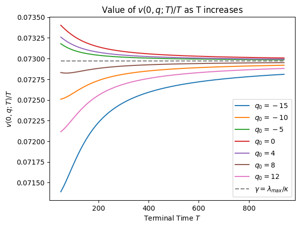
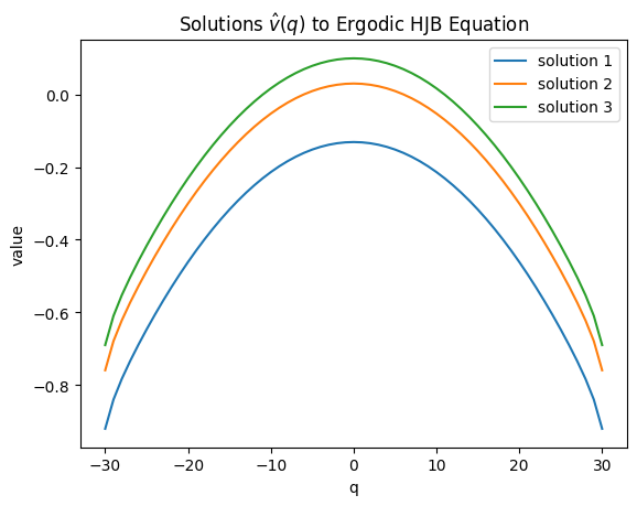
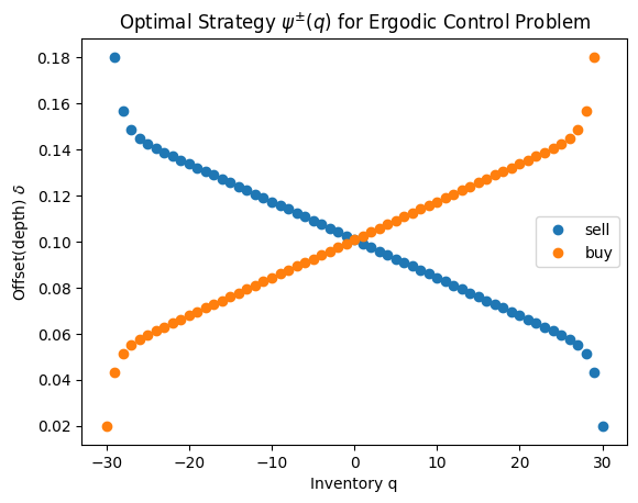
We then solve the ergodic HJB equation (16) and find the optimal feedback control $\psi$. By Theorem 9, there exists the null space of the $n-$square matrix $\bm{C}$ with non-trivial solutions satisfying $\bm{C}\bm{\hat{\omega}}=0$ with $\text{rank}(C)=n-1$. We consider the positive solutions in the null space, hence the solutions $\bm{\hat{v}}=\ln\bm{\hat{\omega}}/\kappa$ to the ergodic HJB equation can be well-defined. Figure 1 (middle panel) represents several solutions $q\mapsto\hat{v}(q)$ to the ergodic HJB equation (16). It can be seen that the solution $\hat{v}(q)$ is unique up to a constant. For all possible solutions $\hat{v}(q)$, the optimal control $\psi^{\pm}(q)$ for the ergodic control problem is unique, as shown in Figure 1 (right panel).

Refer to caption
Refer to caption
Figure 2. Left: Histogram of $Q_{t}$ at $t=1000s$, $1250s$, $1500s$, $1750s$ and $2000s$ under the ergodic optimal control $\psi^{\pm}$. Moreover, the dotted blue line plots the theoretical equilibrium distribution $\pi$ under the ergodic control $\psi^{\pm}$ as derived in Appendix A.10. Right: The log of total variation between the inventory distribution $\pi_{t}$ and the equilibrium $\pi$.

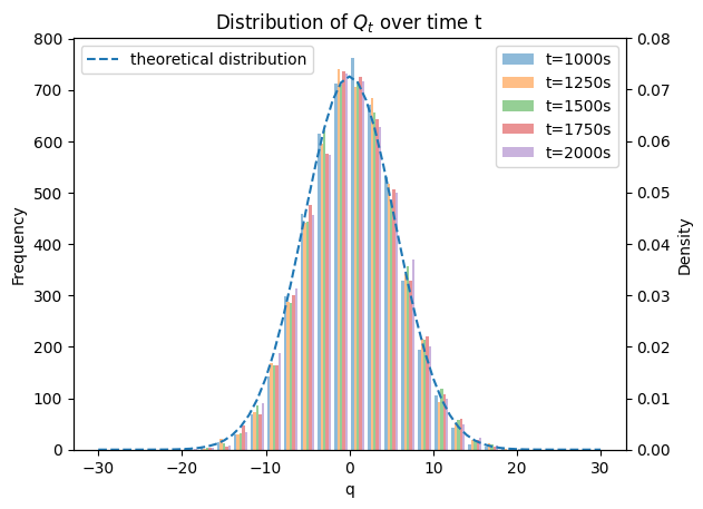
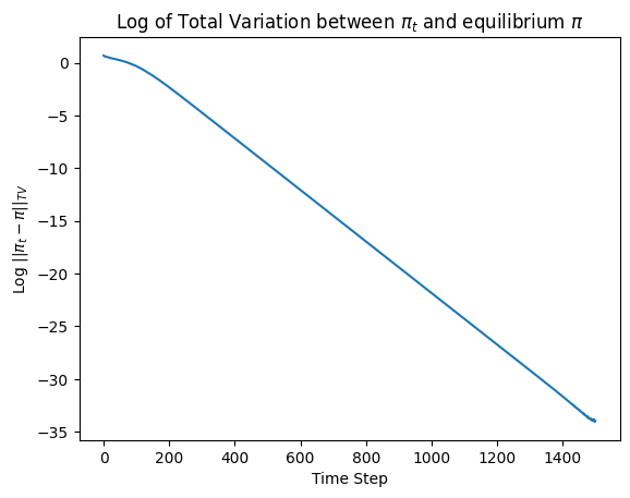
We continue to analyse the ergodicity of the market making system. Figure 2 (left panel) plots the inventory distribution $\pi_{t}$ at time $t=1000s$, $1250s$, $1500s$, $1750s$ and $2000s$ under the ergodic optimal control $\psi^{\pm}$. We can see that the distribution $\pi_{t}$ tends to converge to the dotted blue line over time, which is the theoretical equilibrium distribution $\pi$ of the inventory as derived in Appendix A.10. The right panel in Figure 2 plots the log of the total variation between the distribution $\pi_{t}$ and the equilibrium $\pi$. We terminates the simulation at $t=1500s$ as it reaches the machine precision. It shows that the convergence rate to the equilibrium is exponential.

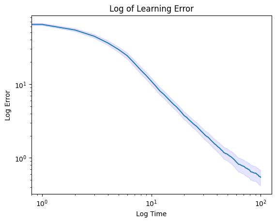
Now we proceed to simulate the proposed learning algorithm for the price sensitivity of market participants parameter $\kappa$ and its achieved regret. Figure 3 (left panel) plots the learning error $\left|\kappa_{t}-\kappa^{\star}\right|$ of Algorithm 1 in the log-log scale. Initially, the learning rate is slow due to the limited number of Bernoulli signals. As time increases, the estimated $\kappa_{t}$ quickly converges to the true parameter $\kappa^{\star}$. Moreover, the right panel of Figure 3, which is the Monte-Carlo simulation of the achieved (expected) regret of Algorithm 1, demonstrates that the algorithm regret grows sublinearly and is bounded by order $\mathcal{O}(\ln^{2}T)$. The complete code can be found at https://github.com/Galen-Cao/MM_parmater_learning.

Refer to caption
Refer to caption
Figure 3. Left: Log-log plot of the learning error $\left|\kappa_{t}-\kappa^{\star}\right|$ over time under Algorithm 1. Right: The regret over time for Algorithm 1.

4. Conclusion

In this paper, we introduced and analysed the ergodic formulation of the Avellaneda–Stoikov market making model. We established explicit solutions to the ergodic Hamilton–Jacobi–Bellman (HJB) equation and thus derived the optimal ergodic Markov controls. We’ve further shown that under the ergodic optimal control there is a unique invariant distribution for the market maker’s inventory and that any initial distribution converges exponentially fast to the equilibrium one. This allowed us to establish the regret upper bound of $\mathcal{O}(\ln^{2}T)$ for learning the unknown price sensitivity of liquidity takers $\kappa^{\star}$. Our work extends the known results on the market making model by providing a rigorous analysis of the ergodic setting and offering a robust solution for parameter learning. The numerical experiments further validate the theoretical results, confirming the robustness of the proposed algorithm.

A number of interesting questions have not been addressed in this paper and are left for future work. In particular, a key extension of the market making framework presented here accounts for adverse selection. Learning the parameters modelling adverse selection and establishing a regret bound would be interesting. Further, it would be interesting to compare this approach to a more classical RL algorithms where the optimal policy is learned directly. One would conjecture that as long as the market is behaving as the model postulates (up to the unknown parameter) using the optimal control derived from the maximum likelihood performs better. However, should the environment deviate from the model it’s possible that the pure RL approach will outperform the method proposed here.

Appendix A Proofs

A.1. Proof of Theorem 1

We first prove the properties of the Hamiltonian function $H$ given by (10).

Lemma 35 (Hamiltonian function).

For the Hamiltonian function $H$, we have

  1. (i)

    $\forall(q,\bm{p})\in\Omega^{Q}\times\mathbb{R}^{2}$, $H(q,\bm{p})$ is finite.

  2. (ii)

    $\forall\bm{p}\in\mathbb{R}^{2}$, $\exists\,\delta^{\pm,*}\in\mathbb{R}^{2}$ such that

    $$H(q,\bm{p})=H(q,\delta^{\pm,*},\bm{p})\,.$$
  3. (iii)

    $p_{1}\mapsto H(q,(p_{1},p_{2})))$ is strictly increasing for any $q\in\Omega^{Q}$ and $p_{2}\in\mathbb{R}$; and $p_{2}\mapsto H(q,(p_{1},p_{2})))$ is strictly increasing for any $q\in\Omega^{Q}$ and $p_{1}\in\mathbb{R}$.

  4. (iv)

    $\bm{p}\mapsto H(q,\bm{p})$ is locally Lipschitz for any $q\in\Omega^{Q}$.

Proof.

(i) (ii) Given $\forall(q,\bm{p})\in\Omega^{Q}\times\mathbb{R}^{2}$, we have

$$\begin{split}H(q,\bm{p})&=\sup_{\delta^{+}\in\mathbb{R}}\Big{\{}\lambda^{+}e^{-\kappa^{+}\delta^{+}}(p_{1}+\delta^{+})\Big{\}}+\sup_{\delta^{-}\in\mathbb{R}}\Big{\{}\lambda^{-}e^{-\kappa^{-}\delta^{-}}(p_{2}+\delta^{-})\Big{\}}-\phi q^{2}\,.\end{split}$$

Consider the function $c(\delta):\delta\mapsto c(\delta)\in\mathbb{R}$ as $c(\delta)=\lambda e^{-\kappa\delta}(p+\delta)$, where $\lambda,\kappa$ and $p$ are given. By letting the first derivative of $c(\delta)$ be 00 and checking that the second derivative is less than 00, we know that $c(\delta)$ attains its supremum at $\delta^{*}=\frac{1}{\kappa}-p$. Therefore, with the fact that $\phi q^{2}\geq 0$,

$$H(q,\bm{p})\leq\lambda^{+}e^{-\kappa^{+}\delta^{+,*}}(p_{1}+\delta^{+,*})+\lambda^{-}e^{-\kappa^{-}\delta^{-,*}}(p_{2}+\delta^{-,*})<+\infty.$$

Moreover, the supremum in the right hand side can be attained at $\delta^{\pm,*}$ given by the above expression, hence the results.

(iii) Given $q\in\Omega^{Q}$ and $p_{2}\in\mathbb{R}$, consider $p_{1}$ and $p^{\prime}_{1}$ such that $p_{1}>p^{\prime}_{1}$. Since $\lambda^{+}e^{-\kappa^{+}\delta^{*}}>0$, we have

$$\begin{split}\lambda^{+}e^{-\kappa^{+}\delta^{+}}(p_{1}+\delta^{+})\bm{1}_{q>\underline{q}}+&\lambda^{-}e^{-\kappa^{-}\delta^{-}}(p_{2}+\delta^{-})\bm{1}_{q<\bar{q}}-\phi q^{2}\,>\,\\ &\lambda^{+}e^{-\kappa^{+}\delta^{+}}(p^{\prime}_{1}+\delta^{+})\bm{1}_{q>\underline{q}}+\lambda^{-}e^{-\kappa^{-}\delta^{-}}(p_{2}+\delta^{-})\bm{1}_{q<\bar{q}}-\phi q^{2}\end{split}$$

By taking the supremum on both sides, we have $H(q,(p_{1},p_{2}))>H(q,(p^{\prime}_{1},p_{2}))$. Similarly, we have $H(q,(p_{1},p_{2}))>H(q,(p_{1},p^{\prime}_{2}))$ if $p_{2}>p^{\prime}_{2}$ given $q\in\Omega^{Q}$ and $p_{1}\in\mathbb{R}$.

(iv) We consider $\bm{p}=(p_{1},p_{2})$ and $\bm{p^{\prime}}=(p^{\prime}_{1},p^{\prime}_{2})$, then

$$\begin{split}\left|H(q,\bm{p})-H(q,\bm{p^{\prime}})\right|&=\bigg{|}\sup_{\delta^{+}\in\mathbb{R}}\Big{\{}\lambda^{+}e^{-\kappa^{+}\delta^{+}}(p_{1}+\delta^{+})\Big{\}}+\sup_{\delta^{-}\in\mathbb{R}}\Big{\{}\lambda^{-}e^{-\kappa^{-}\delta^{-}}(p_{2}+\delta^{-})\Big{\}}\\ &\quad-\sup_{\delta^{+}\in\mathbb{R}}\Big{\{}\lambda^{+}e^{-\kappa^{+}\delta^{+}}(p^{\prime}_{1}+\delta^{+})\Big{\}}-\sup_{\delta^{-}\in\mathbb{R}}\Big{\{}\lambda^{-}e^{-\kappa^{-}\delta^{-}}(p^{\prime}_{2}+\delta^{-})\Big{\}}\bigg{|}\\ &=\left|\frac{\lambda^{+}e^{-1}}{\kappa^{+}}\big{(}e^{-\kappa^{+}p_{1}}-e^{-\kappa^{+}p^{\prime}_{1}}\big{)}+\frac{\lambda^{-}e^{-1}}{\kappa^{-}}\big{(}e^{-\kappa^{-}p_{2}}-e^{-\kappa^{-}p^{\prime}_{2}}\big{)}\right|\,.\end{split}$$

With the fact that $x\mapsto e^{x}$ is locally Lipschitz, we conclude the result. ∎

To prove the existence of the unique solution $u$ to the HJB equation (13) on $(-\infty,T]$, we use Lemma 35 (4) to prove the locally Lipschitz of the ODE and apply [27, Theorem 3.3].

Moreover, by a standard verification argument, we know that $u=v_{r}$, which $v_{r}$ is the value function of the discounted finite-time-horizon control problem (12), hence the result of Theorem 1.

A.2. Proof of Theorem 3

Proof.

We first prove that $f(Q_{t};\delta_{t})$ for any $(Q_{t})_{t\geq 0}$ taking values in $\Omega^{Q}$ and $\delta_{t}^{\pm}\in\mathcal{A}$ is bounded. We know that, by using Lemma 35 (1), there exists a constant $\bar{C}\in\mathbb{R}$ such that,

(33) $$\begin{split}f(Q_{t};\tilde{\delta}_{t}^{\pm})&=\tilde{\delta}_{t}^{+}\lambda^{+}e^{-\kappa^{+}\tilde{\delta}_{t}^{+}}+\tilde{\delta}_{t}^{-}\lambda^{-}e^{-\kappa^{-}\tilde{\delta}_{t}^{-}}-\phi(Q^{\tilde{\delta}^{\pm}}_{t})^{2}\\ &\leq\sup_{\delta^{\pm}\in\mathbb{R}^{2}}\Big{(}\delta^{+}\lambda^{+}e^{-\kappa^{+}\delta^{+}}+\delta^{-}\lambda^{-}e^{-\kappa^{-}\delta^{-}}\Big{)}\\ &\leq\bar{C}\,,\end{split}$$

and by the boundedness from below of the admissible control set $\mathcal{A}$, there exists $\underline{C}\in\mathbb{R}$ such that

(34) $$\begin{split}f(Q_{t};\tilde{\delta}_{t}^{\pm})&\geq\inf_{\delta^{\pm}\in\mathcal{A}}\Big{(}\delta_{t}^{+}\lambda^{+}e^{-\kappa^{+}\delta_{t}^{+}}+\delta_{t}^{-}\lambda^{-}e^{-\kappa^{-}\delta_{t}^{-}}\Big{)}-\phi(\max(\bar{q},\underline{q}))^{2}\\ &\geq\underline{C}\,.\end{split}$$

To see that, $\forall q\in\Omega^{Q}$ and $t\in\mathbb{R}^{+}$, $v_{r}(q)=\lim_{T\rightarrow+\infty}v_{r}(t,q;T)$, we apply [27, Proposition 4.1] by using the running reward function $f$ is bounded. Moreover, by a standard verification argument, we know that $v_{r}$ is the solution to the HJB equation (15), hence the result of Theorem 3. ∎

A.3. Proof of Theorem 4

To prove Theorem 4, we first prove the following lemma.

Lemma 36.

Let $v_{r}(q)$ be given by (14), we have

  1. (i)

    $\exists\,C_{1}\in\mathbb{R}^{+}$ such that $|rv_{r}(q)|\leq C_{1}$ for any $q\in\Omega^{Q}$ and $r\in\mathbb{R}^{+}$.

  2. (ii)

    $\exists\,C_{2}\in\mathbb{R}^{+}$ such that $|v_{r}(\hat{q})-v_{r}(q)|\leq C_{2}|\hat{q}-q|$ for any $q,\hat{q}\in\Omega^{Q}$ and $r\in\mathbb{R}^{+}$.

Proof.

By using the fact that the running reward function $f$ is bounded (33) and (34), we can apply [27, Lemma 4.3(1)] to get statement (i) of the lemma.

To prove statement (ii), we first define the stopping time $\tau(q,\hat{q})$ under a control $\delta^{\pm}\in\mathcal{A}$ as

$$\tau:=\inf\{t\left.\right|Q_{t}^{\delta^{\pm},0,q}=\hat{q}\}\,.$$

With the fact that, for $\forall q,\hat{q}\in\Omega^{Q}$, the transition probability for $\hat{q}$ from $q$, $\bm{P}(q,\hat{q})>0$, we have $\mathbb{E}[Q_{\tau}]<+\infty$. See more detailed discussion in Appendix A.10 for the transition probability matrix.

Let us consider $\delta^{\pm,\epsilon}\in\mathcal{A}[0,\tau]$ with $\epsilon>0$ such that

$$v_{r}(q)-\epsilon\leq\mathbb{E}_{q}\Big{[}\int_{0}^{\tau}e^{-rt}f(Q_{t};\delta^{\pm,\epsilon})\,\mathrm{d}t+e^{-r\tau}v_{r}(\hat{q})\Big{]}\,.$$

By (33) and (34), there exists $\bar{C},\underline{C}$ such that $0\leq f(q;\delta^{\pm})-\underline{C}\leq\bar{C}-\underline{C}$ for any $q\in\Omega^{Q},\delta^{\pm}\in\mathcal{A}$. Therefore, with the fact that $e^{-rt}\leq 1$ for $t\in[0,\tau]$

$$\begin{split}v_{r}(q)-\epsilon-\frac{\underline{C}}{r}&\leq\mathbb{E}_{q}\Big{[}\int_{0}^{\tau}e^{-rt}\big{(}f(Q_{t};\delta^{\pm})-\underline{C}\big{)}\,\mathrm{d}t+e^{-r\tau}\big{(}v_{r}(\hat{q})-\frac{\underline{C}}{r}\big{)}\Big{]}\\ &\leq\mathbb{E}\Big{[}\int_{0}^{\tau}e^{-rt}\big{(}f(Q_{t};\delta^{\pm})-\underline{C}\big{)}\,\mathrm{d}t\Big{]}+\mathbb{E}\big{[}e^{-r\tau}\big{]}\big{(}v_{r}(\hat{q})-\frac{\underline{C}}{r}\big{)}\\ &\leq(\bar{C}-\underline{C})\mathbb{E}[\tau]+v_{r}(\hat{q})-\frac{\underline{C}}{r}\,.\end{split}$$

Therefore,

$$\begin{split}\frac{v_{r}(q)-v_{r}(\hat{q})}{|q-\hat{q}|}&\leq\frac{1}{|q-\hat{q}|}\Big{(}(\bar{C}-\underline{C})\mathbb{E}[\tau]+\epsilon\Big{)}\leq(\bar{C}-\underline{C})\mathbb{E}[\tau]+\epsilon,\quad q,\hat{q}\in\Omega^{Q},q\neq\hat{q}\,.\end{split}$$

Since $\mathbb{E}[\tau]<+\infty$ and $q\in\Omega^{Q}$, by letting $\epsilon\rightarrow 0$, we conclude that $v_{r}(q)-v_{r}(\hat{q})$ is bounded from above. By simply changing the order of $q$ and $\hat{q}$, we conclude the lower boundedness. Hence, we can find $C_{2}\in\mathbb{R}$ such that

$$|v_{r}(\hat{q})-v_{r}(q)|\leq C_{2}|\hat{q}-q|,\quad\forall q,\hat{q}\in\Omega^{Q},r\in\mathbb{R}^{+}\,.$$

Now we are ready to prove Theorem 4.

Proof.

In the proof we follow the ideas from [27, Proposition 4.6, 4.7]. As $\left|rv_{r}(q)\right|\leq C_{1}$ and $\left|v_{r}(q)-v_{r}(0)\right|\leq C_{2}\bar{q}=C^{\prime}_{2},\,\forall q\in\Omega^{Q}$ by Lemma 36, we can consider a sequence $(r_{n})_{n\in\mathbb{N}}$ converging towards 00 such that the sequences $\big{(}r_{n}v_{r_{n}}(q)\big{)}_{n\in\mathbb{N}}$ and $\big{(}v_{r_{n}}(q)-v_{r_{n}}(0)\big{)}_{n\in\mathbb{N}}$ are convergent for $q\in\Omega^{Q}$. Let $\hat{\gamma}(q)$ denote the limit of the sequence $\big{(}r_{n}v_{r_{n}}(q)\big{)}_{n\in\mathbb{N}}$, we have

$$0=\lim_{n\rightarrow+\infty}r_{n}\big{(}v_{r_{n}}(q)-v_{r_{n}}(0)\big{)}=\lim_{n\rightarrow+\infty}r_{n}v_{r_{n}}(q)-\lim_{n\rightarrow+\infty}r_{n}v_{r_{n}}(0)=\hat{\gamma}(q)-\hat{\gamma}(0)\,.$$

Let $\hat{\gamma}\in\mathbb{R}$ be a constant, then $\hat{\gamma}(q)=\hat{\gamma}(0)=\hat{\gamma}$ for any $q\in\Omega^{Q}$.

Next, we prove that $\hat{\gamma}$ is independent of the sequence $(r_{n})_{n\in\mathbb{N}}$. From the HJB equation (15), we have, for the sequence $v_{r_{n}}(q)$,

$$0=-r_{n}v_{r_{n}}(q)+H\Big{(}q,(v_{r_{n}}(q^{\prime})-v_{r_{n}}(q))_{q^{\prime}\in\{q-1,q+1\}}\Big{)},\quad\forall q\in\Omega^{Q}\,.$$

Let $\hat{v}(q)=\lim_{n\rightarrow+\infty}\big{(}v_{r_{n}}(q)-v_{r_{n}}(0)\big{)}$. As the sequence $\big{(}v_{r_{n}}(q)-v_{r_{n}}(0)\big{)}_{n\in\mathbb{N}}$ is convergent, we know that $\hat{v}(q)$ is well defined. Take $n\rightarrow+\infty$ on both sides, we have

(35) $$0=-\hat{\gamma}+H\Big{(}q,(\hat{v}(q^{\prime})-\hat{v}(q))_{q^{\prime}\in\{q-1,q+1\}}\Big{)},\quad\forall q\in\Omega^{Q}\,.$$

We then consider another sequence $(r^{\prime}_{n})_{n\in\mathbb{N}}$ converging towards 00 that leads to another limit $\eta\in\mathbb{R}$ for the sequence $\big{(}r^{\prime}_{n}v_{r^{\prime}_{n}}(q)\big{)}_{n\in\mathbb{N}}$, i.e. $\lim_{n\rightarrow+\infty}r^{\prime}_{n}v_{r^{\prime}_{n}}(q)=\eta,\,\forall q\in\Omega^{Q}$. Let $\hat{w}(q)=\lim_{n\rightarrow+\infty}\big{(}v_{r^{\prime}_{n}}(q)-v_{r^{\prime}_{n}}(0)\big{)}$, then we have

$$0=-\eta+H\Big{(}q,(\hat{w}(q^{\prime})-\hat{w}(q))_{q^{\prime}\in\{q-1,q+1\}}\Big{)},\quad\forall q\in\Omega^{Q}.$$

Let $z(q)=\hat{w}(q)-\hat{v}(q)$. Since the domain for $z(q)$ is bounded, we know that the supremum and infimum exist. Let us denote $\bar{z}=\sup_{q\in\Omega^{Q}}z(q)$, $\underline{z}=\inf_{q\in\Omega^{Q}}z(q)$ and $\epsilon=\frac{\hat{\gamma}-\eta}{\bar{z}-\underline{z}+1}$.

Let us first assume $\hat{\gamma}>\eta$ and prove that $\hat{\gamma}\leq\eta$ by contradiction. By the definition of $\epsilon$, we have, for $\forall q\in\Omega^{Q}$,

$$\begin{split}0\leq\epsilon&(\bar{z}-z(q)+1)\leq\hat{\gamma}-\eta\\ &=H\Big{(}q,(\hat{v}(q^{\prime})-\hat{v}(q))_{q^{\prime}\in\{q-1,q+1\}}\Big{)}-H\Big{(}q,(\hat{w}(q^{\prime})-\hat{w}(q))_{q^{\prime}\in\{q-1,q+1\}}\Big{)}\,.\end{split}$$

Therefore,

$$\begin{split}-\epsilon\hat{w}(q)+H\Big{(}q,(\hat{w}(q^{\prime})-&\hat{w}(q))_{q^{\prime}\in\{q-1,q+1\}}\Big{)}\leq\\ &-\epsilon(\hat{v}(q)+\bar{z}+1)+H\Big{(}q,(\hat{v}(q^{\prime})-\hat{v}(q))_{q^{\prime}\in\{q-1,q+1\}}\Big{)}\,.\end{split}$$

By using the comparison principle, see [27, Lemma 4.4], we know that $\hat{v}(q)+\bar{z}+1\leq\hat{w}(q)$, for $\forall q\in\Omega^{Q}$, which indicates a contradiction with the definition of $\bar{z}$. Hence, we have $\hat{\gamma}\leq\eta$. By simply changing the order of $\hat{\gamma}$ and $\eta$, we can obtain that $\hat{\gamma}\geq\eta$. Therefore, we conclude that $\hat{\gamma}=\eta$, i.e. $\hat{\gamma}$ is independent of the sequence $(r_{n})_{n\in\mathbb{N}}$. ∎

A.4. Proof of Theorem 5

Proof.

Let us define $\mu(t,q)=v_{0}(T-t,q;T)$, then $\mu(t,q)$ satisfies the following equation

(36) $$-\partial_{t}\mu(t,q)+H\Big{(}q,(\mu(t,q^{\prime})-\mu(t,q))_{q^{\prime}\in\{q-1,q+1\}}\Big{)}=0,\quad\forall(t,q)\in[0,+\infty)\times\Omega^{Q}\,,$$

subject to the initial condition $\mu(0,q)=G(q)$ with $G$ given by (11). We consider $U(t,q)=\mu(t,q)-\hat{\gamma}t$ for $(t,q)\in[0,+\infty)\times\Omega^{Q}$ with $\hat{\gamma}$ given in Theorem 4. We proceed to prove that $U(t,q)$ is bounded.

Let us consider $\varphi^{c}(t,q)=\hat{\gamma}t+\hat{v}(q)+c,\,\forall(t,q)\in[0,+\infty)\times\Omega^{Q}$ with the constant $c\in\mathbb{R}$ and $\hat{\gamma}$ given in Theorem 4 and $\hat{v}(q)=\lim_{n\rightarrow+\infty}\big{(}v_{r_{n}}(q)-v_{r_{n}}(0)\big{)}$, where $(r_{n})_{n\in\mathbb{N}}$ is a sequence converging towards 00 such that $\big{(}v_{r_{n}}(q)-v_{r_{n}}(0)\big{)}_{n\in\mathbb{N}}$ is convergent. From the ergodic HJB equation (16), we have,

$$\begin{split}-\partial_{t}\varphi^{c}(t,q)+&H\Big{(}q,(\varphi^{c}(t,q^{\prime})-\varphi^{c}(t,q))_{q^{\prime}\in\{q-1,q+1\}}\Big{)}=\\ &-\hat{\gamma}+H\Big{(}q,(\hat{v}(q^{\prime})-\hat{v}(q))_{q^{\prime}\in\{q-1,q+1\}}\Big{)}=0,\quad\forall(t,q)\in[0,+\infty)\times\Omega^{Q}\,.\end{split}$$

Let us denote $c_{1}=\inf_{q\in\Omega^{Q}}\big{(}G(q)-\hat{v}(q)\big{)}$, where $G(q)$ is the initial condition for the equation (36). Then we have, $\forall q\in\Omega^{Q}$,

$$\varphi^{c_{1}}(0,q)=\hat{v}(q)+\inf_{q\in\Omega^{Q}}\big{(}G(q)-\hat{v}(q)\big{)}\leq G(q)=v(T,q;T)=\mu(0,q)\,.$$

By using the comparison principle (see [27, Proposition 3.2]), we know that $\varphi^{c_{1}}(t,q)\leq\mu(t,q)$ for $(t,q)\in[0,+\infty)\times\Omega^{Q}$. We then consider $c_{2}=\sup_{q\in\Omega^{Q}}\big{(}G(q)-\hat{v}(q)\big{)}$, and clearly $\varphi^{c_{2}}(0,q)\geq\mu(0,q)$. By using the comparison principle again, we have $\varphi^{c_{2}}(t,q)\geq\mu(t,q)$. Therefore,

$$\varphi^{c_{1}}(t,q)\leq\mu(t,q)\leq\varphi^{c_{2}}(t,q),\quad\forall(t,q)\in[0,+\infty)\times\Omega^{Q}\,.$$

By the expression of $\varphi^{c_{1}}$ and $\varphi^{c_{2}}$, we have

$$\hat{v}(q)+c_{1}\leq\mu(t,q)-\hat{\gamma}t=U(t,q)\leq\hat{v}(q)+c_{2}\,.$$

As $q\mapsto\hat{v}(q)$ is well defined that has been proved in Appendix A.3 and $G(q)$ is bounded by definition, we can conclude that $U(t,q)$ is bounded on $(t,q)\in[0,+\infty)\times\Omega^{Q}$.

Now let us consider $U(T,q)=\mu(T,q)-\hat{\gamma}T$ with $T\in[0,+\infty)$. Take the limit $T\rightarrow+\infty$, we have

$$\lim_{T\rightarrow+\infty}\frac{1}{T}\mu(T,q)=\lim_{T\rightarrow+\infty}\frac{1}{T}\big{(}U(T,q)+\hat{\gamma}T\big{)}\,.$$

Since $U(T,q)$ is bounded, therefore

$$\lim_{T\rightarrow+\infty}\frac{1}{T}\mu(T,q)=\hat{\gamma}=\lim_{T\rightarrow+\infty}\frac{1}{T}v_{0}(T-T,q;T)=\lim_{T\rightarrow+\infty}\frac{1}{T}v_{0}(0,q;T)\,,$$

where $v_{0}(0,q;T)$ satisfies the HJB equation (13) with $r=0$

So far we’ve proved that, there exists a constant $\hat{\gamma}\in\mathbb{R}$ such that $\lim_{r\rightarrow 0}rv_{r}(q)=\hat{\gamma}=\lim_{T\rightarrow+\infty}\frac{1}{T}v_{0}(0,q;T)$ for any $q\in\Omega^{Q}$, which addresses one of the challenges in the ergodic control problem [6]. The next step is to prove that $\hat{\gamma}=\gamma$, where $\gamma$ is the ergodic constant defined in the ergodic control problem (9).

By definition, we have

$$\begin{split}\gamma&=\sup_{\delta\in\mathcal{A}}\lim_{T\rightarrow+\infty}\frac{1}{T}\mathbb{E}_{q}\Big{[}\int_{0}^{T}f(Q^{\delta^{\pm}}_{t};\delta^{\pm})\,\mathrm{d}t\Big{]}\\ &\leq\lim_{T\rightarrow+\infty}\sup_{\delta\in\mathcal{A}}\frac{1}{T}\mathbb{E}_{q}\Big{[}\int_{0}^{T}f(Q^{\delta^{\pm}}_{t};\delta^{\pm})\,\mathrm{d}t\Big{]}\\ &=\lim_{T\rightarrow+\infty}\frac{1}{T}v_{0}(0,q;T)=\hat{\gamma}\,.\end{split}$$

By Theorem 9 and Proposition 8, we know that there actually exists an optimal Markov control $\psi^{\pm}\in\mathcal{A}$ such that

$$\begin{split}\hat{\gamma}&=\lim_{T\rightarrow+\infty}\frac{1}{T}\mathbb{E}_{q}\Big{[}\int_{0}^{T}f(Q^{\psi^{\pm}}_{t};\psi^{\pm})\,\mathrm{d}t\Big{]}\\ &\leq\sup_{\delta\in\mathcal{A}}\lim_{T\rightarrow+\infty}\frac{1}{T}\mathbb{E}_{q}\Big{[}\int_{0}^{T}f(Q^{\delta^{\pm}}_{t};\delta^{\pm})\,\mathrm{d}t\Big{]}=\gamma\,,\end{split}$$

hence $\hat{\gamma}=\gamma$, and all $\hat{\gamma}$ will be substituted by $\gamma$ in the later context. ∎

A.5. Proof of Theorem 6

Proof.

By Theorem 2, the solution to $\bm{v}_{0}(0;T)$ can be given by $\bm{v}_{0}(0;T)=\frac{1}{\kappa}\ln(e^{T\bm{A}}\cdot\bm{z})$. As the subdiagonal and the superdiagonal elements of $\bm{A}$ are $\lambda^{-}e^{-1}$, $\lambda^{+}e^{-1}>0$, we can find a real and symmetric tridiagonal matrix $\bm{J}$ whose entries are given by

(37) $\displaystyle\bm{J}_{ij}=\begin{cases}\bm{A}_{ij},&\text{if $i=j$},\\ \sqrt{\lambda^{+}\lambda^{-}}e^{-1},&\text{if i = j-1 or j+1},\\ 0,&\text{otherwise}\end{cases}$

which is similar to $\bm{A}$. Hence, by [36], $\bm{J}$ (and $\bm{A}$) can be diagonalised with distinct eigenvalues. Let $n=\bar{q}-\underline{q}+1$, $\lambda_{1},\lambda_{2},...,\lambda_{n}$ be $n$ real eigenvalues of $\bm{A}$ with $\lambda_{1}>\lambda_{2}>...>\lambda_{n}$ and $\bm{\Lambda}$ be the diagonal matrix of $\bm{A}$ such that $\bm{A}=\bm{P}^{-1}\bm{\Lambda}\bm{P}$, where $\bm{P}$’s columns are the corresponding eigenvectors.

By Theorem 5, we have

$$\lim_{T\rightarrow+\infty}\frac{1}{T}v_{0}(0,q;T)=\gamma,\quad\forall q\in\Omega^{Q}\,.$$

Therefore, by considering the vector form of $\bm{v}_{0}(0;T)$ and using Theorem 2, we obtain

$$\begin{split}\lim_{T\rightarrow\infty}\frac{\bm{v}_{0}(t=0;T)}{T}&=\frac{1}{\kappa}\lim_{T\rightarrow\infty}\frac{1}{T}\ln(e^{T\bm{A}}\cdot\bm{z})=\frac{1}{\kappa}\lim_{T\rightarrow\infty}\frac{1}{T}\ln(\sum_{i=0}^{\infty}\frac{(T\bm{A})^{n}}{n!}\cdot\bm{z})\\ &=\frac{1}{\kappa}\lim_{T\rightarrow\infty}\frac{1}{T}\ln(\bm{P}e^{T\bm{\Lambda}}\bm{P}^{-1}\cdot\bm{z})\,.\end{split}$$

Let us denote $\bm{P}=\begin{bmatrix}P_{11}&...&P_{1n}\\ P_{21}&...&P_{2n}\\ \vdots&...&\vdots\\ P_{n1}&...&P_{nn}\end{bmatrix}_{n\times n}$ and $\bm{P}^{-1}\cdot\bm{z}=\begin{bmatrix}K_{1}\\ \vdots\\ K_{n}\end{bmatrix}_{n\times 1}$, then

$$\begin{split}\lim_{T\rightarrow\infty}\frac{\bm{v}_{0}(t=0;T)}{T}&=\frac{1}{\kappa}\lim_{T\rightarrow\infty}\frac{1}{T}\ln\begin{bmatrix}\sum_{i=1}^{n}K_{1}P_{1i}e^{\lambda_{i}T}\\ \sum_{i=1}^{n}K_{2}P_{2i}e^{\lambda_{i}T}\\ \vdots\\ \sum_{i=1}^{n}K_{n}P_{ni}e^{\lambda_{i}T}\end{bmatrix}_{n\times 1}\\ &=\frac{1}{\kappa}[\lambda_{1},\lambda_{1},...,\lambda_{1}]^{\top}\,,\end{split}$$

hence the result.

A.6. Proof of Lemma 23

Proof.

As discussed in Appendix A.5, we can find a real and symmetric tridiagonal matrix $\bm{J}$ that is similar to $\bm{A}$, whose eigenvalues are simple, i.e. the algebraic multiplicity is $1$. Moreover, it is obvious that $\kappa\mapsto\bm{J}(\kappa)$ given by (37) is $C^{\infty}([\underline{K},\bar{K}])$. By [30, 32, 41], $\kappa\mapsto\lambda_{max}(\kappa)$ can be parameterised smoothly on $\kappa\in[\underline{K},\bar{K}]$, i.e. $\lambda_{max}(\kappa)$ is $C^{\infty}([\underline{K},\bar{K}])$. By Theorem 6, we know that $\gamma(\kappa)=\frac{\lambda_{max}(\kappa)}{\kappa}$. Therefore, we can conclude that $\gamma(\kappa)$ is $C^{2}([\underline{K},\bar{K}])$ and $\frac{\mathrm{d}^{2}}{\mathrm{d}\kappa^{2}}_{\kappa}\gamma(\kappa)$ is bounded on the compact set $\kappa\in[\underline{K},\bar{K}]$. ∎

A.7. Proof of Proposition 7

Proof.

To prove Proposition 7, we recommend to follow the idea in [27, Proposition 4.7] and use the properties of the Hamiltonian function $H$ in Lemma 35. ∎

A.8. Proof of Proposition 8

Proof.

Notice that the right hand side of

(38) $$\psi^{\pm}(q)\in\operatorname*{arg\,max}_{\delta^{\pm}}H\Big{(}q,(\hat{v}(q^{\prime})-\hat{v}(q))_{q^{\prime}\in\{q-1,q+1\}}\Big{)},\quad\forall q\in\Omega^{Q},$$

is invariant under constant shifts in the solution $\hat{v}$ and hence the optimal control $\psi^{\pm}$ for the ergodic control problem is uniquely given by expression (18) by simply solving the right hand side of (38) with the convention that $\psi^{\pm}(q)=+\,\infty$ for $q=\underline{q},\bar{q}$, respectively. Moreover from (10) it is easy to see that $\psi^{\pm}$ is single-valued and given by the result. ∎

A.9. Proof of Theorem 9

Proof.

By Proposition 8, the ergodic HJB equation (16) can be rewritten as

$$\begin{split}0=-\phi q^{2}-\gamma&+\frac{\lambda^{+}}{\kappa}\exp{\big{(}-1-\kappa\hat{v}(q)+\kappa\hat{v}(q-1)\big{)}}\bm{1}_{q>\underline{q}}\\ &+\frac{\lambda^{-}}{\kappa}\exp{\big{(}-1-\kappa\hat{v}(q)+\kappa\hat{v}(q+1)\big{)}}\bm{1}_{q<\bar{q}}\,.\end{split}$$

By using Theorem 6, we get an explicit solution for $\gamma=\frac{\lambda_{max}}{\kappa}$. Therefore, to solve the ergodic HJB equation, the next step is to solve $\hat{v}$. Let $\hat{v}(q)=\frac{1}{\kappa}\ln\hat{\omega}(q)$, then

(39) $$-\kappa(\phi q^{2}+\gamma)+\lambda^{+}e^{-1}\frac{\hat{\omega}(q-1)}{\hat{\omega}(q)}\bm{1}_{q>\underline{q}}+\lambda^{-}e^{-1}\frac{\hat{\omega}(q+1)}{\hat{\omega}(q)}\bm{1}_{q<\bar{q}}=0\,.$$

Let $n=(\bar{q}-\underline{q}+1)$, $\bm{\hat{\omega}}=[\hat{\omega}(\bar{q}),\hat{\omega}(\bar{q}-1),...,\hat{\omega}(\underline{q})]^{\top}$ be an $n$-dim vector and $\bm{C}$ be an $n$ - square matrix given by

$\displaystyle\bm{C}=\begin{bmatrix}-\kappa(\phi\bar{q}^{2}+\gamma)&\lambda^{+}e^{-1}&0&&&...&\\ \lambda^{-}e^{-1}&-\kappa\big{(}\phi(\bar{q}-1)^{2}+\gamma\big{)}&\lambda^{+}e^{-1}&&&...&\\ &&&...&\\ &...&&&\lambda^{-}e^{-1}&-\kappa\big{(}\phi(\underline{q}+1)^{2}+\gamma\big{)}&\lambda^{+}e^{-1}\\ &...&&&0&\lambda^{-}e^{-1}&-\kappa(\phi\underline{q}^{2}+\gamma)\end{bmatrix}$

Therefore, the equation (39) can be written in a matrix form as

(40) $$\bm{C}\bm{\hat{\omega}}=0\,.$$

By the fact of $\gamma=\frac{\lambda_{max}}{\kappa}$, we observe that $\bm{C}=\bm{A}-\lambda_{max}\bm{I}$, where the matrix $\bm{A}$ is given in Theorem 2, $\lambda_{max}$ is the largest eigenvalue of $\bm{A}$ and $\bm{I}$ is the identity matrix. As $\bm{A}$ has $n$ distinct eigenvalues as proved in Appendix A.5, hence $\text{rank}(\bm{C})=n-1$. Therefore, $\bm{\hat{\omega}}$ is the set of non-trivial solutions to the homogeneous equation (40) with the coefficient matrix $\bm{C}$. ∎

A.10. Proof of Lemma 11

Proof.

Given the ergodic optimal control $\psi(q),\,\forall q\in\Omega^{Q}$, we consider the dynamic of inventory process (4) as a discrete Markov chain. Let $\bm{P}$ be an $n-$square matrix labelled from $\bar{q}$ to $\underline{q}$ denoting the state transition matrix. The entries of $\bm{P}$ are

(41) $\displaystyle\bm{P}_{ij}=\begin{cases}1-\lambda^{+}e^{-\kappa\psi^{+}(i)},&\text{if $i=j=\bar{q}$},\\ 1-\lambda^{-}e^{-\kappa\psi^{-}(i)},&\text{if $i=j=\underline{q}$},\\ 1-\lambda^{+}e^{-\kappa\psi^{+}(i)}-\lambda^{-}e^{-\kappa\psi^{-}(i)}+2\lambda^{+}\lambda^{-}e^{-\kappa(\psi^{+}(i)+\psi^{-}(i))},&\text{if $i=j\neq\bar{q},\underline{q}$},\\ \lambda^{-}e^{-\kappa\psi^{-}(i)}(1-\lambda^{+}e^{-\kappa\psi^{+}(i)}),&\text{if $i=j-1\neq\underline{q}$},\\ \lambda^{+}e^{-\kappa\psi^{+}(i)}(1-\lambda^{-}e^{-\kappa\psi^{-}(i)}),&\text{if $i=j+1\neq\bar{q}$},\\ \lambda^{-}e^{-\kappa\psi^{-}(i)},&\text{if $i=j-1=\underline{q}$},\\ \lambda^{+}e^{-\kappa\psi^{+}(i)},&\text{if $i=j+1=\bar{q}$},\\ 0,&\text{otherwise}.\end{cases}$

From the discussion for the tridiagonal matrix in Appendix A.5, clearly $\bm{P}$ is diagonalisable. Let $\lambda_{1},\lambda_{2},...,\lambda_{n}$ be $n$ real eigenvalues of $\bm{P}$. Let $\bm{\Lambda}$ be the diagonal matrix of $\bm{P}$ with $\bm{\Lambda}=\bm{U}^{-1}\bm{P}\bm{U}$, where $\bm{U}$’s columns are the eigenvectors of $\bm{P}$. As $\bm{P}$ is a stochastic matrix, hence by Perron–Frobenius theorem,

$$1=\lambda_{1}>|\lambda_{2}|>...>|\lambda_{n}|.$$

Therefore, given an initial distribution $\bm{q}$, the equilibrium $\bm{\pi}$ under $\delta^{*,\pm}$ as $T$ goes to infinity is

$$\begin{split}\bm{\pi}&=\lim_{T\rightarrow+\infty}\bm{q}\bm{P}^{T}\\ &=\bm{q}\lim_{T\rightarrow+\infty}\bm{U}\bm{\Lambda}^{T}\bm{U}^{-1}\\ &=\bm{q}\bm{U}\bm{W}\bm{U}^{-1}\,,\end{split}$$

with $\bm{W}$ an $n-$square matrix with only $1$ on the first diagonal element and 00 otherwise

A.11. Proof of Lemma 17

Proof.

The equation (24) is a step in the proof of Theorem 27 in a simpler case. We know that $\psi^{\kappa^{\star}}$ is the optimal control for the ergodic market making model under $\kappa^{\star}$ satisfying (18). Hence, from the ergodic HJB equation (16), we have

$$\begin{split}0=-\gamma(\kappa^{\star})-\phi q^{2}+&\lambda^{+}e^{-\kappa^{\star}\psi^{\kappa^{\star},+}(q)}\Big{(}\hat{v}^{\kappa^{\star}}(q-1)-\hat{v}^{\kappa^{\star}}(q)+\psi^{\kappa^{\star},+}(q)\Big{)}\bm{1}_{q>\underline{q}}\\ +&\lambda^{-}e^{-\kappa^{\star}\psi^{\kappa^{\star},-}(q)}\Big{(}\hat{v}^{\kappa^{\star}}(q+1)-\hat{v}^{\kappa^{\star}}(q)+\psi^{\kappa^{\star},-}(q)\Big{)}\bm{1}_{q<\bar{q}}\,.\end{split}$$

Therefore,

$$\begin{split}\gamma(\kappa^{\star})=\lambda^{+}\psi^{\kappa^{\star},+}(q)e^{-\kappa^{\star}\psi^{\kappa^{\star},+}(q)}&+\lambda^{-}\psi^{\kappa^{\star},-}(q)e^{-\kappa^{\star}\psi^{\kappa^{\star},-}(q)}-\phi q^{2}\\ &+\lambda^{+}e^{-\kappa^{\star}\psi^{\kappa^{\star},+}(q)}\big{(}\hat{v}^{\kappa^{\star}}(q-1)-\hat{v}^{\kappa^{\star}}(q)\big{)}\bm{1}_{q>\underline{q}}\\ &+\lambda^{-}e^{-\kappa^{\star}\psi^{\kappa^{\star},-}(q)}\big{(}\hat{v}^{\kappa^{\star}}(q+1)-\hat{v}^{\kappa^{\star}}(q)\big{)}\bm{1}_{q<\bar{q}}\,,\end{split}$$

where we ignore the indicator functions in the first line and use $\psi^{\kappa^{\star},\pm}(q)e^{-\kappa^{\star}\psi^{\kappa^{\star},\pm}(q)}=0$ for $q=\bar{q},\underline{q}$ respectively. Moreover, we notice that the first line satisfies (21), therefore

$$\begin{split}\bigg{|}\gamma(\kappa^{\star})T-\mathbb{E}_{q}\Big{[}&\int_{0}^{T}f(Q_{t}^{\psi^{\kappa^{\star}};\kappa^{\star}},\psi^{\kappa^{\star}};\kappa^{\star})\,\mathrm{d}t\Big{]}\bigg{|}\\ &=\bigg{|}\mathbb{E}_{q}\Big{[}\int_{0}^{T}\big{(}\gamma(\kappa^{\star})-f(Q_{t}^{\psi^{\kappa^{\star}};\kappa^{\star}},\psi^{\kappa^{\star}};\kappa^{\star})\big{)}\,\mathrm{d}t\Big{]}\bigg{|}\\ &=\bigg{|}\mathbb{E}_{q}\Big{[}\int_{0}^{T}\Big{(}\lambda^{+}e^{-\kappa^{\star}\psi^{\kappa^{\star},+}(q)}\big{(}\hat{v}^{\kappa^{\star}}(q-1)-\hat{v}^{\kappa^{\star}}(q)\big{)}\bm{1}_{q>\underline{q}}\\ &\qquad\qquad\qquad\quad+\lambda^{-}e^{-\kappa^{\star}\psi^{\kappa^{\star},-}(q)}\big{(}\hat{v}^{\kappa^{\star}}(q+1)-\hat{v}^{\kappa^{\star}}(q)\big{)}\bm{1}_{q<\bar{q}}\Big{)}\,\mathrm{d}t\Big{]}\bigg{|}\,.\end{split}$$

Let $\pi^{\kappa^{\star}}$ denote the equilibrium of the optimal ergodic market making model under parameter $\kappa^{\star}$ and function $h$ be

$$\begin{split}h(\kappa^{\star},q)=\lambda^{+}e^{-\kappa^{\star}\psi^{\kappa^{\star},+}(q)}\big{(}\hat{v}^{\kappa^{\star}}(q-1)&-\hat{v}^{\kappa^{\star}}(q)\big{)}\bm{1}_{q>\underline{q}}\\ &+\lambda^{-}e^{-\kappa^{\star}\psi^{\kappa^{\star},-}(q)}\big{(}\hat{v}^{\kappa^{\star}}(q+1)-\hat{v}^{\kappa^{\star}}(q)\big{)}\bm{1}_{q<\bar{q}}\,.\end{split}$$

By Lemma 36 (2), $h$ is bounded by $\bar{h}\in\mathbb{R}^{+}$. From a simpler version of Proposition 26 by substituting $\psi^{\kappa}$ to $\psi^{\kappa^{\star}}$, Lemma 12 and Lemma 36 (2), we have

$$\begin{split}\bigg{|}\gamma(\kappa^{\star})T-\mathbb{E}_{q}\Big{[}&\int_{0}^{T}f(Q_{t}^{\psi^{\kappa^{\star}};\kappa^{\star}},\psi^{\kappa^{\star}};\kappa^{\star})\,\mathrm{d}t\Big{]}\bigg{|}\\ &=\bigg{|}\int_{0}^{T}\int_{\Omega^{Q}}\Big{(}\lambda^{+}e^{-\kappa^{\star}\psi^{\kappa^{\star},+}(q)}\big{(}\hat{v}^{\kappa^{\star}}(q-1)-\hat{v}^{\kappa^{\star}}(q)\big{)}\bm{1}_{q>\underline{q}}\\ &\qquad\qquad\qquad\quad+\lambda^{-}e^{-\kappa^{\star}\psi^{\kappa^{\star},-}(q)}\big{(}\hat{v}^{\kappa^{\star}}(q+1)-\hat{v}^{\kappa^{\star}}(q)\big{)}\bm{1}_{q<\bar{q}}\Big{)}\,\mathrm{d}t\,\mathrm{d}\pi^{\kappa^{\star}}_{t}\bigg{|}\\ &\leq\bigg{|}\bar{h}\int_{0}^{T}\int_{\Omega^{Q}}\frac{h(\kappa^{\star},q)}{\bar{h}}(\mathrm{d}\pi^{\kappa^{\star}}_{t}-\mathrm{d}\pi^{\kappa^{\star}})\,\mathrm{d}t\bigg{|}\\ &\leq\bar{h}\int_{0}^{T}\left\|\pi^{\kappa^{\star}}_{t}-\pi^{\kappa^{\star}}\right\|_{TV}\,\mathrm{d}t\leq\frac{\bar{h}C}{-\ln\alpha}\,,\end{split}$$

with constants $C>0$ and $0<\alpha<1$ independent of $T$, hence the result. ∎

A.12. Proof of Lemma 20

Proof.

Let $w(t,q)$ satisfy the linear ODE (29) subject to the terminal condition (11), i.e.

$$0=\partial_{t}w(t,q)-rw(t,q)+H\Big{(}q,\psi^{\kappa},(w(t,q^{\prime})-w(t,q))_{q^{\prime}\in\{q-1,q+1\}};\kappa^{\star}\Big{)},\,\forall q\in\Omega^{Q},$$

and $w(T,q)=G(q)$. Clearly, the equation (29) is a linear ODE, hence there exists $\bm{w}\in C^{1}([0,T];\mathbb{R}^{n})$, which is a solution to (29).

Let us consider the following stochastic process, and we omit the superscript for $Q_{t}^{\psi^{\kappa};\kappa^{\star}}$ for notational simplicity.

$$X(s)=e^{-r(s-t)}w(s,Q_{s})+\int_{t}^{s}e^{-r(u-t)}f(Q_{u},\psi^{\kappa}_{u};\kappa^{\star})\,\mathrm{d}u$$

We know that $Q_{t}^{\psi^{\kappa};\kappa^{\star}}$ follows the SDE (4) with market parameter $\kappa^{\star}$ and control $\psi^{\kappa}$, i.e.

$$\begin{split}dQ_{t}^{\psi^{\kappa};\kappa^{\star}}&=dN_{t}^{\psi^{\kappa},-}-dN_{t}^{\psi^{\kappa},+}\\ &=\big{(}\lambda^{+}e^{-\kappa^{\star}\psi^{\kappa,-}}-\lambda^{-}e^{-\kappa^{\star}\psi^{\kappa,+},}\big{)}dt+d\tilde{N}_{t}^{\psi^{\kappa},-}-d\tilde{N}_{t}^{\psi^{\kappa},+},\end{split}$$

where $\tilde{N}_{t}^{\psi^{\kappa},\pm}$ are compensated Poisson processes.

By Itô’s formula,

$\displaystyle dX(s)=\,e^{-r(s-t)}\Big{\{}\partial_{s}w(s,Q_{s})-rw(s,Q_{s})+\lambda^{+}e^{-\kappa^{\star}\psi^{\kappa,+}}\left(w(s,Q_{s}-1)-w(s,Q_{s})\right)\bm{1}_{Q_{s}>\underline{q}}$
$\displaystyle+\lambda^{-}e^{-\kappa^{\star}\psi^{\kappa,-}}\left(w(s,Q_{s}+1)-w(s,Q_{s})\right)\bm{1}_{Q_{s}<\bar{q}}+f(Q_{s},\psi^{\kappa};\kappa^{\star})\Big{\}}ds$
$\displaystyle+e^{-r(s-t)}\Big{\{}\left(w(s,Q_{s}-1)-w(s,Q_{s})\right)\bm{1}_{Q_{s}>\underline{q}}d\tilde{N}_{s}^{+}+\left(w(s,Q_{s}+1)-w(s,Q_{s})\right)\bm{1}_{Q_{s}<\bar{q}}d\tilde{N}_{s}^{-}\Big{\}}$
$\displaystyle=\,e^{-r(s-t)}\Big{\{}\partial_{s}w(s,Q_{s})-rw(s,Q_{s})+H\big{(}Q_{s},\psi^{\kappa},(w(s,Q_{s}^{\prime})-w(s,Q_{s}))_{Q_{s}^{\prime}\in\{Q_{s}-1,Q_{s}+1\}}\big{)}\Big{\}}ds$
$\displaystyle+e^{-r(s-t)}\Big{\{}\left(w(s,Q_{s}-1)-w(s,Q_{s})\right)\bm{1}_{Q_{s}>\underline{q}}d\tilde{N}_{s}^{+}+\left(w(s,Q_{s}+1)-w(s,Q_{s})\right)\bm{1}_{Q_{s}<\bar{q}}d\tilde{N}_{s}^{-}\Big{\}}.$

where the last equality comes from the definition of $H(\cdot;\kappa^{\star})$ (27) and $f(\cdot;\kappa^{\star})$ (21). Take the integral and expectation for $X(s)$, we have

$$\begin{split}\mathbb{E}\big{[}&X(T)\big{|}Q_{t}=q\big{]}=\mathbb{E}\big{[}X(t)\big{|}Q_{t}=q\big{]}\\ &+\int_{t}^{T}e^{-r(s-t)}\Big{(}\partial_{s}w-rw+H\big{(}Q_{s},\psi^{\kappa},(w(s,Q^{\prime}_{s})-w(s,Q_{s}))_{Q^{\prime}_{s}\in\{Q_{s}-1,Q_{s}+1\}}\big{)}\Big{)}\,\mathrm{d}s\\ \end{split}$$

As $w(t,q)$ satisfies (29) and the terminal condition (11), therefore,

$$\begin{split}w(t,q)=\mathbb{E}\big{[}X(t)\big{|}Q_{t}=q\big{]}&=\mathbb{E}\big{[}X(T)\big{|}Q_{t}=q\big{]}\\ &=\mathbb{E}_{q}\Big{[}\int_{t}^{T}e^{-r(u-t)}f(Q_{u},\psi^{\kappa};\kappa^{\star})\,\mathrm{d}u+e^{-r(T-t)}G(Q_{T})\Big{]}.\end{split}$$

Hence $w(t,q)=v_{r}^{\psi^{\kappa}}(t,q;T;\kappa^{\star})$ by (28). ∎

A.13. Proof of Proposition 21

Proof.

First, let $v_{r}^{\psi^{\kappa}}(q;\kappa^{\star})$ be the expected reward in the discounted infinite-time-horizon setting, where the true price sensitivity parameter is $\kappa^{\star}$ but the market maker uses the strategy $\psi^{\kappa}$ given by (18) with parameter $\kappa$, i.e.

(42) $$v_{r}^{\psi^{\kappa}}(q;\kappa^{\star})=\mathbb{E}_{q}\Big{[}\int_{0}^{+\infty}e^{-rt}f(Q_{t}^{\psi^{\kappa};\kappa^{\star}},\psi^{\kappa};\kappa^{\star})\,\mathrm{d}t\Big{]},$$

where $f(\cdot;\kappa^{\star})$ is given by (21). Then we claim that $v_{r}^{\psi^{\kappa}}(q;\kappa^{\star})$ satisfies the following linear system

(43) $$0=-rv_{r}^{\psi^{\kappa}}(q;\kappa^{\star})+H\Big{(}q,\psi^{\kappa},(v_{r}^{\psi^{\kappa}}(q^{\prime};\kappa^{\star})-v_{r}^{\psi^{\kappa}}(q;\kappa^{\star}))_{q^{\prime}\in\{q-1,q+1\}};\kappa^{\star}\Big{)},\quad\forall q\in\Omega^{Q}\,.$$

We would like to provide a sketch of proof for the claim. First, the existence of $v_{r}^{\psi^{\kappa}}(q;\kappa^{\star})$ defined by (42) can follow the proof in Section A.2 for Theorem 3 but substituting the Hamiltonian function $H$ (10) for $H(\cdot;\kappa^{\star})$ (27). Let $w(q)$ be a solution for the linear system (43). Consider

$$X(s)=e^{-rs}w(Q_{s})+\int_{0}^{s}e^{-rt}f(Q_{t},\psi^{\kappa};\kappa^{\star})\,\mathrm{d}t\,.$$

By Itô’s formula

$\displaystyle dX(s)=$ $\displaystyle\,e^{-rs}\Big{\{}-rw(Q_{s})+\lambda^{+}e^{-\kappa^{\star}\psi^{\kappa,+}_{s}}\left(w(Q_{s}-1)-w(Q_{s})\right)\bm{1}_{Q_{s}>\underline{q}}$
$\displaystyle\quad+\lambda^{-}e^{-\kappa^{\star}\psi^{\kappa,-}_{s}}\left(w(Q_{s}+1)-w(Q_{s})\right)\bm{1}_{Q_{s}<\bar{q}}+f(Q_{s},\psi^{\kappa};\kappa^{\star})\Big{\}}ds$
$\displaystyle+e^{-rs}\Big{\{}\left(w(Q_{s}-1)-w(Q_{s})\right)\bm{1}_{Q_{s}>\underline{q}}d\tilde{N}_{s}^{+}+\left(w(Q_{s}+1)-w(Q_{s})\right)\bm{1}_{Q_{s}<\bar{q}}d\tilde{N}_{s}^{-}\Big{\}}$
$\displaystyle=$ $\displaystyle\,e^{-rs}\Big{\{}-rw(Q_{s})+H\left(Q_{s},\psi^{\kappa},(w(Q^{\prime}_{s})-w(Q_{s}))_{Q^{\prime}_{s}\in\{Q_{s}-1,Q_{s}+1\}}\right)\Big{\}}ds$
$\displaystyle+e^{-rs}\Big{\{}\left(w(Q_{s}-1)-w(Q_{s})\right)\bm{1}_{Q_{s}>\underline{q}}d\tilde{N}_{s}^{+}+\left(w(Q_{s}+1)-w(Q_{s})\right)\bm{1}_{Q_{s}<\bar{q}}d\tilde{N}_{s}^{-}\Big{\}}.$

where the last equality comes from the definition of $H(\cdot;\kappa^{\star})$ (27) and $f(\cdot;\kappa^{\star})$ (21). Take the integral and expectation for $X(s)$, we have

$$\begin{split}\mathbb{E}\big{[}X(T)\big{|}Q_{0}=q\big{]}&=\mathbb{E}\big{[}X(0)\big{|}Q_{0}=q\big{]}\\ &+\int_{0}^{T}e^{-rt}\Big{(}-rw(Q_{t})+H\big{(}Q_{t},\psi^{\kappa},(w(Q_{t}^{\prime})-w(Q_{t}))_{Q_{t}^{\prime}\in\{Q_{t}-1,Q_{t}+1\}}\big{)}\Big{)}\,\mathrm{d}t\\ \end{split}$$

As $w(q)$ satisfies (43), therefore,

$$\begin{split}w(q)=\mathbb{E}\big{[}X(0)\big{|}Q_{0}=q\big{]}&=\mathbb{E}\big{[}X(T)\big{|}Q_{0}=q\big{]}\\ &=\mathbb{E}_{q}\Big{[}\int_{0}^{T}e^{-rt}f(Q_{t},\psi^{\kappa};\kappa^{\star})\,\mathrm{d}t+e^{-rT}w(Q_{T})\Big{]}.\end{split}$$

Take limit $T\rightarrow+\infty$ on both sides, with the fact that the limit exists, i.e. $w(q)\in\mathbb{R},\forall q\in\Omega^{Q}$

$$w(q)=\mathbb{E}_{q}\Big{[}\int_{0}^{+\infty}e^{-rt}f(Q_{t},\psi^{\kappa};\kappa^{\star})\,\mathrm{d}t\Big{]}.$$

Hence $w(q)=v_{r}^{\psi^{\kappa}}(q;\kappa)$ defined by (42).

Now, we would like to to show that given $\gamma(\kappa;\kappa^{\star})$ defined by (30), it holds that

(44) $$\lim_{r\rightarrow 0}rv_{r}^{\psi^{\kappa}}(q;\kappa^{\star})=\gamma(\kappa;\kappa^{\star}),\quad\forall q\in\Omega^{Q}\,,$$

where $v_{r}^{\psi^{\kappa}}(q;\kappa^{\star})$ is defined by (42).

Let us start with the following lemma.

Lemma 37.
  1. (1)

    $\exists\,C_{1}\in\mathbb{R}^{+}$ such that $\left|rv_{r}^{\psi^{\kappa}}(q;\kappa^{\star})\right|\leq C_{1}$ for $\forall q\in\Omega^{Q}$ and $r\in\mathbb{R}^{+}$.

  2. (2)

    $\exists\,C_{2}\in\mathbb{R}^{+}$ such that $\left|v_{r}^{\psi^{\kappa}}(\hat{q};\kappa^{\star})-v_{r}^{\psi^{\kappa}}(q;\kappa^{\star})\right|\leq C_{2}|\hat{q}-q|$ for $\forall q,\hat{q}\in\Omega^{Q}$ and $r\in\mathbb{R}^{+}$.

As $\psi^{\kappa}\subset\mathcal{A}$, i.e. the collection of all Markov controls optimal for the ergodic control problem is a subset of the admissible control, the running reward function $f(\cdot;\kappa^{\star})$ is bounded. By (21), we have

(45) $$\begin{split}f(Q_{t},\psi^{\kappa};\kappa^{\star})&=\lambda^{+}\psi^{\kappa,+}e^{-\kappa^{\star}\psi^{\kappa,+}}+\lambda^{-}\psi^{\kappa,-}e^{-\kappa^{\star}\psi^{\kappa,-}}-\phi(Q_{t})^{2}\\ &\leq\sup_{\psi^{\kappa}\in\overline{\mathbb{R}}^{2}}\big{(}\lambda^{+}\psi^{\kappa,+}e^{-\kappa^{\star}\psi^{\kappa,+}}+\lambda^{-}\psi^{\kappa,-}e^{-\kappa^{\star}\psi^{\kappa,-}}\big{)}\\ &=\overline{C}\,\end{split}$$

and by the boundedness from below of $\mathcal{A}$,

(46) $$\begin{split}f(Q_{t},\psi^{\kappa};\kappa^{\star})&=\lambda^{+}\psi^{\kappa,+}e^{-\kappa^{\star}\psi^{\kappa,+}}+\lambda^{-}\psi^{\kappa,-}e^{-\kappa^{\star}\psi^{\kappa,-}}-\phi(Q_{t})^{2}\\ &\geq\inf_{\psi^{\kappa}}\big{(}\lambda^{+}\psi^{\kappa,+}e^{-\kappa^{\star}\psi^{\kappa,+}}+\lambda^{-}\psi^{\kappa,-}e^{-\kappa^{\star}\psi^{\kappa,-}}\big{)}-\phi\max(\bar{q},\underline{q})^{2}\\ &=\underline{C}\,.\end{split}$$

To prove Lemma 37 (1), we first consider that

$$\begin{split}v_{r}^{\psi^{\kappa}}(q;\kappa^{\star})&=\mathbb{E}_{q}\Big{[}\int_{0}^{+\infty}e^{-rt}f(Q_{t}^{\psi^{\kappa};\kappa^{\star}},\psi^{\kappa};\kappa^{\star})\,\mathrm{d}t\Big{]}\geq\mathbb{E}_{q}\Big{[}\int_{0}^{+\infty}e^{-rt}\underline{C}\,\mathrm{d}t\Big{]}=\frac{\underline{C}}{r}\,.\end{split}$$

On the other hand,

$$\begin{split}v_{r}^{\psi^{\kappa}}(q;\kappa^{\star})\leq\mathbb{E}_{q}\Big{[}\int_{0}^{+\infty}e^{-rt}\overline{C}\,\mathrm{d}t\Big{]}=\frac{\bar{C}}{r}\,.\end{split}$$

Hence

$$\left|rv_{r}(q)\right|\leq C_{1},\,\forall q\in\Omega^{Q},$$

with $C_{1}=\max(\left|\underline{C}\right|,\left|\overline{C}\right|)$.

To prove Lemma 37 (2), we define the stopping time $\tau(q,\hat{q})$ for $Q_{t}^{\psi^{\kappa};\kappa^{\star}}$ with $Q_{0}=q$ as

$$\tau:=\inf\{t\left.\right|Q_{t}^{\psi^{\kappa};\kappa^{\star}}=\hat{q}\}\,.$$

With the fact that, $\forall q,\hat{q}\in\Omega^{Q}$, the transition probability for $\hat{q}$ from $q$, i.e. $\bm{P}(q,\hat{q})>0$, see the more detailed discussion in Section A.10, it implies that $\mathbb{E}[Q_{\tau}]<+\infty$.

By (45) and (46), there exists $\overline{C},\underline{C}$ such that $0\leq f(q;\psi^{\kappa};\kappa^{\star})-\underline{C}\leq\overline{C}-\underline{C}$ for any $q\in\Omega^{Q}$. Therefore,

$$\begin{split}v_{r}^{\psi^{\kappa}}(q;\kappa^{\star})-\frac{\underline{C}}{r}&=\mathbb{E}_{q}\Big{[}\int_{0}^{\tau}e^{-rt}\big{(}f(Q^{\psi^{\kappa};\kappa^{\star}}_{t},\psi^{\kappa};\kappa^{\star})-\underline{C}\big{)}\,\mathrm{d}t+e^{-r\tau}\big{(}v_{r}^{\psi^{\kappa}}(\hat{q};\kappa^{\star})-\frac{\underline{C}}{r}\big{)}\Big{]}\\ &\leq\mathbb{E}\Big{[}\int_{0}^{\tau}e^{-rt}\big{(}\overline{C}-\underline{C}\big{)}\,\mathrm{d}t\Big{]}+\mathbb{E}\big{[}e^{-r\tau}\big{]}\big{(}v^{\psi^{\kappa};\kappa^{\star}}_{r}(\hat{q})-\frac{\underline{C}}{r}\big{)}\\ &\leq(\bar{C}-\underline{C})\mathbb{E}[\tau]+v^{\psi^{\kappa};\kappa^{\star}}_{r}(\hat{q})-\frac{\underline{C}}{r}\,.\end{split}$$

Therefore,

$$\begin{split}\frac{v^{\psi^{\kappa};\kappa^{\star}}_{r}(q)-v^{\psi^{\kappa};\kappa^{\star}}_{r}(\hat{q})}{|q-\hat{q}|}&\leq\frac{1}{|q-\hat{q}|}\Big{(}(\bar{C}-\underline{C})\mathbb{E}[\tau]\Big{)}\leq(\bar{C}-\underline{C})\mathbb{E}[\tau],\,\forall q,\hat{q}\in\Omega^{Q},q\neq\hat{q}.\end{split}$$

Since $\mathbb{E}[\tau]<+\infty$, we conclude that $\frac{v^{\psi^{\kappa};\kappa^{\star}}_{r}(q)-v^{\psi^{\kappa};\kappa^{\star}}_{r}(\hat{q})}{|q-\hat{q}|}$ is bounded from above. By simply changing the order of $q$ and $\hat{q}$, we conclude the lower boundedness. Hence, we can find $C_{2}\in\mathbb{R}^{+}$ such that

$$\left|v^{\psi^{\kappa};\kappa^{\star}}_{r}(q)-v^{\psi^{\kappa};\kappa^{\star}}_{r}(\hat{q})\right|\leq C_{2}|\hat{q}-q|,\,\forall q,\hat{q}\in\Omega^{Q},r\in\mathbb{R}^{+}\,.$$

.

With the fact that $\Big{|}rv_{r}^{\psi^{\kappa}}(q;\kappa^{\star})\Big{|}$ and $\Big{|}v_{r}^{\psi^{\kappa}}(\hat{q};\kappa^{\star})-v_{r}^{\psi^{\kappa}}(q;\kappa^{\star})\Big{|}$ are bounded, we can follow the discussion in Appendix A.3, i.e. consider a sequence $(r_{n})_{n\in\mathbb{N}}$ converging towards 00 such that the sequences $\big{(}r_{n}v_{r_{n}}^{\psi^{\kappa};\kappa^{\star}}(q)\big{)}_{n\in\mathbb{N}}$ and $\big{(}v_{r_{n}}^{\psi^{\kappa};\kappa^{\star}}(q)-v_{r_{n}}^{\psi^{\kappa};\kappa^{\star}}(0)\big{)}_{n\in\mathbb{N}}$ are convergent for $\forall q\in\Omega^{Q}$, then show that there exists $\gamma(\kappa;\kappa^{\star})\in\mathbb{R}$ such that $\gamma(\kappa;\kappa^{\star})=\lim_{r\rightarrow 0}rv_{r}^{\psi^{\kappa}}(q;\kappa^{\star})$. Again by substituting $H$ (10) for $H(\cdot;\kappa^{\star})$ in the proof of Theorem 5 in Appendix A.4, we can easily conclude that $\gamma(\kappa;\kappa^{\star})$ given by (44) also satisfies

$$\gamma(\kappa;\kappa^{\star})=\lim_{T\rightarrow+\infty}\frac{1}{T}v_{0}^{\psi^{\kappa}}(t=0,q;T;\kappa^{\star})\,.$$

Let us define $\hat{v}^{\psi^{\kappa}}(q;\kappa^{\star})=\lim_{r\rightarrow 0}\big{(}v_{r}^{\psi^{\kappa}}(q;\kappa^{\star})-v_{r}^{\psi^{\kappa}}(0;\kappa^{\star})\big{)}$ for $q\in\Omega^{Q}$. By the convergent of $\big{(}v_{r_{n}}^{\psi^{\kappa};\kappa^{\star}}(q)-v_{r_{n}}^{\psi^{\kappa};\kappa^{\star}}(0)\big{)}_{n\in\mathbb{N}}$ under the sequence $(r_{n})_{n\in\mathbb{N}}$ converging towards 00, we know that $\hat{v}^{\psi^{\kappa}}(q;\kappa^{\star})$ is well defined.

By passing the limit (44) to the equation (43), we obtain that

$$0=-\gamma(\kappa;\kappa^{\star})+H\Big{(}q,\psi^{\kappa},(\hat{v}^{\psi^{\kappa},\kappa^{\star}}(q^{\prime})-\hat{v}^{\psi^{\kappa},\kappa^{\star}}(q))_{q^{\prime}\in\{q-1,q+1\}};\kappa^{\star}\Big{)}\,,\,\forall q\in\Omega^{Q}.$$

A.14. Proof of Proposition 22

Proof.

By (29), the linear ODE for $t\mapsto v_{r}^{\psi^{\kappa}}(t,q;T;\kappa^{\star})$ can be written in a matrix form. Let $\bm{v}_{r}(t)=[v_{r}^{\psi^{\kappa}}(t,\bar{q};T;\kappa^{\star}),...,v_{r}^{\psi^{\kappa}}(t,\underline{q};T;\kappa^{\star})]$ be an $n-dim$ vector, where $n=\bar{q}-\underline{q}+1$. Now, let $\bm{\tilde{A}}_{r}$ denote an $n$-square matrix whose rows are labelled from $\bar{q}$ to $\underline{q}$ and entries are given by

(47) $\displaystyle\bm{\tilde{A}}_{r}(i,q)=\begin{cases}-(r+\lambda^{+}e^{-\kappa^{\star}\psi^{\kappa,+}(q)}\bm{1}_{q>\underline{q}}+\lambda^{-}e^{-\kappa^{\star}\psi^{\kappa,-}(q)}\bm{1}_{q<\bar{q}}),&\text{if $i=q$},\\ \lambda^{+}e^{-\kappa^{\star}\psi^{\kappa,+}(q)},&\text{if $i=q+1$},\\ \lambda^{-}e^{-\kappa^{\star}\psi^{\kappa,-}(q)},&\text{if $i=q-1$},\\ 0,&\text{otherwise. }\end{cases}$

Let $\bm{\tilde{b}}$ be an $n-dim$ vector where each component is

(48) $$b_{i}=\lambda^{+}\psi^{\kappa,+}(i)e^{-\kappa^{\star}\psi^{\kappa,+}(i)}\bm{1}_{i>\underline{q}}+\lambda^{-}\psi^{\kappa,-}(i)e^{-\kappa^{\star}\psi^{\kappa,-}(i)}\bm{1}_{i<\bar{q}}-\phi i^{2},$$

for $i=[\bar{q},\bar{q}-1,...,\underline{q}]$. Then $t\mapsto\bm{v}_{r}(t)$ satisfies

(49) $$0=\partial_{t}\bm{v}_{r}(t)+\bm{\tilde{A}}_{r}(\kappa)\bm{v}_{r}(t)+\bm{\tilde{b}}(\kappa),$$

with the terminal condition $\bm{v}_{r}(T;q)=[G(\bar{q}),\ldots,G(\underline{q})]^{\top}$, with $G$ given by (11). Let $\bm{G}$ denote the vector $[G(\bar{q}),\ldots,G(\underline{q})]^{\top}$. We know that there exists a solution to the linear ODE (49) with the terminal condition on $t\in(-\infty,T]$.

Now, let us consider the case of $r=0$. We use $\bm{\tilde{A}}_{0}(,i)$ to denote the $i-$th column of the coefficient matrix $\bm{\tilde{A}}_{0}$ with $i\in\{1,2,\dots,n\}$. With the entries given by (47) under $r=0$, we can observe that

$$\sum_{i=1}^{n-1}\bm{\tilde{A}}_{0}(,i)=-\bm{\tilde{A}}_{0}(,n),$$

which means $\bm{\tilde{A}}_{0}$ is singular. Hence the solution to (49) under $r=0$ can be given by

(50) $$\bm{v}_{0}(t)=e^{(T-t)\bm{\tilde{A}}_{0}(\kappa)}\bm{G}+\int_{t}^{T}e^{(s-t)\bm{\tilde{A}}_{0}(\kappa)}\bm{\tilde{b}}(\kappa)\,\mathrm{d}s.$$

By (47), $\bm{\tilde{A}}_{0}$ is a real tridiagonal matrix with all positive off-diagonal entries. Clearly the eigenvalues of $\bm{\tilde{A}}_{0}$ are simple, i.e. the algebraic multiplicity is 1. Furthermore, $\bm{\tilde{A}}_{0}$ is diagonally dominant matrix with all negative diagonal entries, i.e.

$$-\bm{\tilde{A}}_{0}(i,i)=\bm{\tilde{A}}_{0}(i,i-1)+\bm{\tilde{A}}_{0}(i,i-1)>0,$$

then $\bm{\tilde{A}}_{0}(i,i-1)$ is negative semi-definite. Let $\lambda_{i},i=\{1,\dots,n\}$ be the eigenvalues of $\bm{\tilde{A}}_{0}$ with $\lambda_{n}<\lambda_{n-1}<\dots<\lambda_{1}=0$, $\bm{U}$ be the matrix whose columns are the corresponding eigenvectors and $\bm{\Lambda}$ be the diagonal matrix. Then

$$\begin{split}\lim_{T\rightarrow+\infty}\frac{1}{T}\bm{v}_{0}(0,T)&=\lim_{T\rightarrow+\infty}\frac{1}{T}e^{T\bm{\tilde{A}}_{0}(\kappa)}\bm{G}+\lim_{T\rightarrow+\infty}\frac{1}{T}\int_{0}^{T}e^{t\bm{\tilde{A}}_{0}(\kappa)}\bm{\tilde{b}}(\kappa)\,\mathrm{d}t\\ &=\lim_{T\rightarrow+\infty}\frac{1}{T}\bm{U}e^{T\bm{\Lambda}}\bm{U}^{-1}\bm{G}+\lim_{T\rightarrow+\infty}\frac{1}{T}\bm{U}\int_{0}^{T}e^{t\bm{\Lambda}}\,\mathrm{d}t\,\bm{U}^{-1}\bm{\tilde{b}}\\ &=\lim_{T\rightarrow+\infty}\frac{1}{T}\bm{U}\begin{bmatrix}e^{\lambda_{1}T}&&&&\\ &e^{\lambda_{2}T}&&&&\\ &&&\dots&\\ &&&&&e^{\lambda_{n}T}\end{bmatrix}\bm{U}^{-1}\bm{G}\\ &\quad+\lim_{T\rightarrow+\infty}\frac{1}{T}\bm{U}\begin{bmatrix}\int_{0}^{T}e^{\lambda_{1}t}\,\mathrm{d}t&&&&\\ &\int_{0}^{T}e^{\lambda_{2}t}\,\mathrm{d}t&&&&\\ &&&\dots&\\ &&&&&\int_{0}^{T}e^{\lambda_{n}t}\,\mathrm{d}t\end{bmatrix}\bm{U}^{-1}\bm{\tilde{b}}\\ &=\lim_{T\rightarrow+\infty}\frac{1}{T}\bm{U}\begin{bmatrix}T&&&&\\ &\frac{1}{\lambda_{2}}(e^{\lambda_{2}T}-1)&&&&\\ &&&\dots&\\ &&&&&\frac{1}{\lambda_{n}}(e^{\lambda_{n}T}-1)\end{bmatrix}\bm{U}^{-1}\bm{\tilde{b}}\\ &=\bm{U}\bm{W}\bm{U}^{-1}\bm{\tilde{b}}\,,\end{split}$$

where $\bm{W}$ is the $n-$square matrix with only $1$ on the first diagonal element and 00 otherwise. By (30), we know $\gamma(\kappa;\kappa^{\star})\mathds{1}=\bm{U}\bm{W}\bm{U}^{-1}\bm{\tilde{b}}$ with $\mathds{1}$ the $n-$dim vector with all entries $1$. ∎

A.15. Proof of Lemma 24

Proof.

First, we would like to prove that $\kappa\mapsto\psi^{\kappa}$ with $\psi^{\kappa}$ given by 18 is $C^{\infty}([\underline{K},\bar{K}])$. By Proposition 8 and Theorem 9, it is equivalent to show that $\kappa\mapsto\bm{\hat{\omega}}(\kappa)$ by (19) is $C^{\infty}([\underline{K},\bar{K}])$. Let us consider a matrix $\bm{D}$ as

(51) $$\bm{D}=Diag(\,d_{\bar{q}},d_{\bar{q}-1},\dots,d_{\underline{q}}\,),$$

with $d_{q}=\prod_{\bar{q}-1,\dots,q}\sqrt{\frac{\lambda^{-}}{\lambda^{+}}}$ for $q\in\{\bar{q}-1,\bar{q}-2,\dots,\underline{q}\}$ and $d_{\bar{q}}=1$. Then $\bm{C}$ given in Theorem 9 can be transformed into a real and symmetric tridiagonal matrix $\bm{\tilde{C}}$ by $\bm{\tilde{C}}=\bm{D}^{-1}\bm{C}\bm{D}$ with entries

(52) $\displaystyle\bm{\tilde{C}}(i,q)=\begin{cases}-\kappa\phi q^{2}-\kappa\gamma(\kappa),&\text{if $i=q$},\\ \sqrt{\lambda^{+}\lambda^{-}}e^{-1},&\text{if $i=q-1$ or $q+1$},\\ 0,&\text{otherwise.}\end{cases}$

As there exists an $\bm{\hat{\omega}}$ solves (19), there must be an eigenvalue $\lambda_{1}=0$ of $\bm{C}$, or $\bm{\tilde{C}}$ as they are similar, with the corresponding eigenvector $\bm{\hat{\omega}}$ of $\bm{C}$ and $\bm{\tilde{\omega}}$ of $\bm{\tilde{C}}$. Therefore,

(53) $$0=\lambda_{1}\bm{\tilde{\omega}}=\bm{\tilde{C}}\bm{\tilde{\omega}}=\bm{D}^{-1}\bm{C}\bm{D}\bm{\tilde{\omega}}.$$

As $\bm{D}$ is non-singular, we have $\bm{\hat{\omega}}=\bm{D}\bm{\tilde{\omega}}$. As shown in Appendix A.6, $\gamma(\kappa)$ is $C^{\infty}([\underline{K},\bar{K}])$, therefore $\kappa\mapsto\bm{\tilde{C}}(\kappa)$ given by (52) is $C^{\infty}([\underline{K},\bar{K}])$. Hence, by [5, Result 7.2; Theorem 7.6], the eigenvector $\bm{\tilde{\omega}}$ can be parameterised smoothly on $\kappa\in[\underline{K},\bar{K}]$. Obviously, $\bm{D}$ is independent of $\kappa$. Therefore, we can conclude that $\bm{\hat{\omega}}(\kappa)=\bm{D}\bm{\tilde{\omega}}(\kappa)$ is $C^{\infty}([\underline{K},\bar{K}])$.

Proposition 22 gives an analytical solution to $\gamma(\kappa;\kappa^{\star})$ but it is not enough to show $\kappa\mapsto\gamma(\kappa;\kappa^{\star})$ is twice differentiable, as $\bm{U}$’s columns are the eigenvectors of $\bm{\tilde{A}}_{0}$ whereas $\bm{\tilde{A}}_{0}$ is not a self-adjoint or normal operator. Let us consider the matrix $\bm{V}$ as

(54) $$\bm{V}=Diag(\,v_{\bar{q}},v_{\bar{q}-1},\dots,v_{\underline{q}}\,),$$

with $v_{q}=\frac{\prod_{i=\bar{q}-1}^{q}\sqrt{\lambda^{-}}e^{-\frac{1}{2}\kappa^{\star}\psi^{\kappa,-}(i)}}{\prod_{i=\bar{q}}^{q+1}\sqrt{\lambda^{+}}e^{-\frac{1}{2}\kappa^{\star}\psi^{\kappa,+}(i)}}$ for $q\in\{\bar{q}-1,\bar{q}-2,\dots,\underline{q}\}$ and $v_{\bar{q}}=1$. Then $\bm{J}=\bm{V}^{-1}\bm{\tilde{A}}_{0}\bm{V}$ is a real and symmetric tridiagonal matrix with the entries as

(55) $\displaystyle\bm{J}(i,q)=\begin{cases}-(\lambda^{+}e^{-\kappa^{\star}\psi^{\kappa,+}(q)}\bm{1}_{q>\underline{q}}+\lambda^{-}e^{-\kappa^{\star}\psi^{\kappa,-}(q)}\bm{1}_{q<\bar{q}}),&\text{if $i=q$},\\ \sqrt{\lambda^{+}\lambda^{-}}e^{-\frac{\kappa^{\star}}{\kappa}},&\text{if $i=q+1$},\\ \sqrt{\lambda^{+}\lambda^{-}}e^{-\frac{\kappa^{\star}}{\kappa}},&\text{if $i=q-1$},\\ 0,&\text{otherwise. }\end{cases}$

There exists an orthogonal matrix $\bm{U^{\prime}}$ whose columns are the eigenvectors of $\bm{J}$ such that $\bm{\Lambda}=\bm{U^{\prime}}^{-1}\bm{J}\bm{U^{\prime}}$, where $\bm{\Lambda}$ is the diagonal matrix with eigenvalues of $\bm{\tilde{A}}_{0}$ since $\bm{J}$ is similar to $\bm{\tilde{A}}_{0}$. Moreover, we have

$$\bm{\Lambda}=\bm{U^{\prime}}^{-1}\bm{J}\bm{U^{\prime}}=\bm{U^{\prime}}^{-1}\bm{V}^{-1}\bm{\tilde{A}}_{0}\bm{V}\bm{U^{\prime}}=\bm{U}^{-1}\bm{\tilde{A}}_{0}\bm{U},$$

hence $\bm{U}=\bm{V}\bm{U^{\prime}}$. Therefore,

$$\gamma(\kappa;\kappa^{\star})\mathds{1}=\bm{V}\bm{U^{\prime}}\bm{W}\bm{U^{\prime}}^{-1}\bm{V}^{-1}\bm{\tilde{b}}.$$

Let $\bm{U^{\prime}}=[\bm{u}_{1},\bm{u}_{2},\dots,\bm{u}_{n}]$ where $\bm{u}_{i}$ is the corresponding eigenvector of $\bm{J}$ with the eigenvalue $\lambda_{i}$. Then

$$\bm{U^{\prime}}\bm{W}\bm{U^{\prime}}^{-1}=Diag(\bm{u}_{1})\bm{W^{\prime}}Diag(\bm{u}_{1}),$$

where $\bm{W^{\prime}}$ is the $n-$square matrix with all entries $1$ and $\bm{u}_{1}$ is the eigenvector of $\bm{J}$ with $\lambda_{1}=0$.

(56) $$\gamma(\kappa;\kappa^{\star})\mathds{1}=\bm{V}Diag(\bm{u}_{1})\bm{W^{\prime}}Diag(\bm{u}_{1})\bm{V}^{-1}\bm{\tilde{b}}.$$

Clearly, $\psi^{\kappa}\mapsto e^{-\kappa^{\star}\psi^{\kappa}}$ is a smooth function and $\kappa\mapsto\psi^{\kappa}$ is $C^{\infty}([\underline{K},\bar{K}])$. Therefore, $\bm{V}(\kappa)$ (54), $\bm{V}^{-1}(\kappa)$, $\bm{\tilde{b}}(\kappa)$ (48) and $\bm{J}(\kappa)$ are $C^{\infty}([\underline{K},\bar{K}])$. Moreover, $\bm{J}$ is a real and symmetric tridiagonal matrix with the simple eigenvalue $\lambda_{1}$. By [5, Result 7.2; Theorem 7.6], we know that $\kappa\mapsto\bm{u}_{1}(\kappa)$ can be chosen to be parameterised smoothly in $\kappa$. Hence, by (56), $\kappa\mapsto\gamma(\kappa;\kappa^{\star})$ is at least $C^{2}([\underline{K},\bar{K}])$ and $\frac{\mathrm{d}^{2}}{\mathrm{d}\kappa^{2}}_{\kappa}\gamma(\kappa;\kappa^{\star})$ is bounded on the compact set $\kappa\in[\underline{K},\bar{K}]$. ∎

A.16. Proof of Proposition 26

Proof.

By Proposition 21 and by (27), the equation (31) can be expressed as

$$\begin{split}\gamma(\kappa;\kappa^{\star})=-\phi q^{2}+&\lambda^{+}e^{-\kappa^{\star}\psi^{\kappa,+}(q)}\Big{(}\hat{v}^{\psi^{\kappa}}(q-1;\kappa^{\star})-\hat{v}^{\psi^{\kappa}}(q;\kappa^{\star})+\psi^{\kappa,+}(q)\Big{)}\bm{1}_{q>\underline{q}}\\ +&\lambda^{-}e^{-\kappa^{\star}\psi^{\kappa,-}(q)}\Big{(}\hat{v}^{\psi^{\kappa}}(q+1;\kappa^{\star})-\hat{v}^{\psi^{\kappa}}(q;\kappa^{\star})+\psi^{\kappa,-}(q)\Big{)}\bm{1}_{q<\bar{q}}\,.\end{split}$$

Take integral from 00 to $T$ and then take the expectation with respect to the probability measure $\pi^{\psi^{\kappa};\kappa^{\star}}$ under the controlled SDE (22) with $Q_{0}\sim\pi^{\psi^{\kappa};\kappa^{\star}}$, we have

$\displaystyle\int_{\Omega^{Q}}\int_{0}^{T}\gamma(\kappa;\kappa^{\star})\,\mathrm{d}t\,\mathrm{d}\pi^{\psi^{\kappa};\kappa^{\star}}=\int_{\Omega^{Q}}\int_{0}^{T}\Big{(}\lambda^{+}\psi^{\kappa,+}(q)e^{-\kappa^{\star}\psi^{\kappa,+}(q)}+\lambda^{-}\psi^{\kappa,-}(q)e^{-\kappa^{\star}\psi^{\kappa,-}(q)}$
$\displaystyle-\phi q^{2}+\lambda^{+}e^{-\kappa^{\star}\psi^{\kappa,+}}\big{(}\hat{v}^{\psi^{\kappa}}(q-1;\kappa^{\star})-\hat{v}^{\psi^{\kappa}}(q;\kappa^{\star})\big{)}\bm{1}_{q>\underline{q}}$
$\displaystyle+\lambda^{-}e^{-\kappa^{\star}\psi^{\kappa,-}}\big{(}\hat{v}^{\psi^{\kappa}}(q+1;\kappa^{\star})-\hat{v}^{\psi^{\kappa}}(q;\kappa^{\star})\big{)}\bm{1}_{q<\bar{q}}\Big{)}\,\mathrm{d}t\,\mathrm{d}\pi^{\psi^{\kappa};\kappa^{\star}}\,,$

where we omit the indicator function in the first line since $\psi^{\kappa,\pm}(q)e^{-\kappa^{\star}\psi^{\kappa,\pm}(q)}=0$ when $q=\bar{q},\underline{q}$, respectively. As $\gamma(\kappa;\kappa^{\star})$ is independent of $q$ and $t$ by Proposition 21, dividing by $T>0$ we get

$$\begin{split}&\gamma(\kappa;\kappa^{\star})\\ &=\frac{1}{T}\mathbb{E}_{\pi^{\psi^{\kappa};\kappa^{\star}}}\Big{[}\int_{0}^{T}\lambda^{+}\psi^{\kappa,+}e^{-\kappa^{\star}\psi^{\kappa,+}(Q_{t}^{\psi^{\kappa};\kappa^{\star}})}+\lambda^{-}\psi^{\kappa,-}e^{-\kappa^{\star}\psi^{\kappa,-}(Q_{t}^{\psi^{\kappa};\kappa^{\star}})}-\phi(Q_{t}^{\psi^{\kappa};\kappa^{\star}})^{2}\,\mathrm{d}t\Big{]}\\ &\qquad+\frac{1}{T}\int_{\Omega^{Q}}\int_{0}^{T}\Big{(}\lambda^{+}e^{-\kappa^{\star}\psi^{\kappa,+}(q)}\big{(}\hat{v}^{\psi^{\kappa}}(q-1;\kappa^{\star})-\hat{v}^{\psi^{\kappa}}(q;\kappa^{\star})\big{)}\bm{1}_{q>\underline{q}}\\ &\qquad\qquad+\lambda^{-}e^{-\kappa^{\star}\psi^{\kappa,-}(q)}\big{(}\hat{v}^{\psi^{\kappa}}(q+1;\kappa^{\star})-\hat{v}^{\psi^{\kappa}}(q;\kappa^{\star})\big{)}\bm{1}_{q<\bar{q}}\Big{)}\,\mathrm{d}t\,\mathrm{d}\pi^{\psi^{\kappa};\kappa^{\star}}.\end{split}$$

Moreover, for the initial distribution $\pi^{\psi^{\kappa};\kappa^{\star}}$, we have

$$\begin{split}&\gamma(\kappa;\kappa^{\star})=\lim_{T\rightarrow+\infty}\frac{1}{T}v_{0}^{\psi^{\kappa}}(t=0,q;T;\kappa^{\star})\\ &=\lim_{T\rightarrow+\infty}\frac{1}{T}\mathbb{E}_{\pi^{\psi^{\kappa};\kappa^{\star}}}\Big{[}\int_{0}^{T}\Big{(}\lambda^{+}\psi^{\kappa,+}e^{-\kappa^{\star}\psi^{\kappa,+}}+\lambda^{-}\psi^{\kappa,-}e^{-\kappa^{\star}\psi^{\kappa,-}}-\phi(Q^{\psi^{\kappa};\kappa^{\star}}_{t})^{2}\Big{)}\,\mathrm{d}t\Big{]}\end{split}$$

Hence

$$\begin{split}0=\int_{\Omega^{Q}}\lambda^{+}e^{-\kappa^{\star}\psi^{\kappa,+}}\Big{(}&\hat{v}^{\psi^{\kappa}}(q-1;\kappa^{\star})-\hat{v}^{\psi^{\kappa}}(q;\kappa^{\star})\Big{)}\bm{1}_{q>\underline{q}}\\ &+\lambda^{-}e^{-\kappa^{\star}\psi^{\kappa,-}}\Big{(}\hat{v}^{\psi^{\kappa}}(q+1;\kappa^{\star})-\hat{v}^{\psi^{\kappa}}(q;\kappa^{\star})\Big{)}\bm{1}_{q<\bar{q}}\,\mathrm{d}\pi^{\psi^{\kappa};\kappa^{\star}},\end{split}$$

which concludes the proof. ∎

A.17. Proof of Theorem 27

Proof.

By (31) in Proposition 21 and (27), we have,

$$\begin{split}\lambda^{+}\psi^{\kappa,+}(q)e^{-\kappa^{\star}\psi^{\kappa,+}(q)}+\lambda^{-}\psi^{\kappa,-}(q)&e^{-\kappa^{\star}\psi^{\kappa,-}(q)}-\phi q^{2}=\\ \gamma(\kappa;\kappa^{\star})&+\lambda^{+}e^{-\kappa^{\star}\psi^{\kappa,+}}\big{(}\hat{v}^{\psi^{\kappa}}(q-1;\kappa^{\star})-\hat{v}^{\psi^{\kappa}}(q;\kappa^{\star})\big{)}\bm{1}_{q>\underline{q}}\\ &+\lambda^{-}e^{-\kappa^{\star}\psi^{\kappa,-}}\big{(}\hat{v}^{\psi^{\kappa}}(q+1;\kappa^{\star})-\hat{v}^{\psi^{\kappa}}(q;\kappa^{\star})\big{)}\bm{1}_{q<\bar{q}},\end{split}$$

where we ignore the indicator functions in the first line since $\psi^{\kappa,\pm}(q)e^{-\kappa^{\star}\psi^{\kappa,\pm}(q)}=0$ for $q=\bar{q},\underline{q}$, respectively. Also, by definition, we know that

$$f(t,q,\delta^{\pm};\kappa^{\star})=\lambda^{+}\delta^{+}e^{-\kappa^{\star}\delta^{+}}+\lambda^{-}\delta^{-}e^{-\kappa^{\star}\delta^{-}}-\phi q^{2}.$$

Therefore, by Definition 16 of regret,

(57) $$\begin{split}&\mathcal{R}^{\Psi}(T)=\gamma(\kappa^{\star})T-\mathbb{E}_{q}\Big{[}\int_{0}^{T}f(t,Q_{t}^{\psi^{\kappa_{t}};\kappa^{\star}},\psi^{\kappa_{t}};\kappa^{\star})\,\mathrm{d}t\Big{]}\\ &=\mathbb{E}\Big{[}\int_{0}^{T}\big{(}\gamma(\kappa^{\star};\kappa^{\star})-\gamma(\kappa_{t};\kappa^{\star})\big{)}\,\mathrm{d}t\Big{]}\\ &\,\,\,\,-\mathbb{E}_{q}\Big{[}\int_{0}^{T}\lambda^{+}e^{-\kappa^{\star}\psi^{\kappa_{t},+}(Q_{t}^{\psi^{\kappa_{t}};\kappa^{\star}})}\Big{(}\hat{v}^{\psi^{\kappa_{t}}}(Q_{t}^{\psi^{\kappa_{t}};\kappa^{\star}}-1;\kappa^{\star})-\hat{v}^{\psi^{\kappa_{t}}}(Q_{t}^{\psi^{\kappa_{t}};\kappa^{\star}};\kappa^{\star})\Big{)}\bm{1}_{Q_{t}^{\psi^{\kappa_{t}};\kappa^{\star}}>\underline{q}}\\ &\quad\quad+\lambda^{-}e^{-\kappa^{\star}\psi^{\kappa_{t},-}(Q_{t}^{\psi^{\kappa_{t}};\kappa^{\star}})}\Big{(}\hat{v}^{\psi^{\kappa_{t}}}(Q_{t}^{\psi^{\kappa_{t}};\kappa^{\star}}+1;\kappa^{\star})-\hat{v}^{\psi^{\kappa_{t}}}(Q_{t}^{\psi^{\kappa_{t}};\kappa^{\star}};\kappa^{\star})\Big{)}\bm{1}_{Q_{t}^{\psi^{\kappa_{t}};\kappa^{\star}}<\bar{q}}\,\mathrm{d}t\Big{]}\,.\\ \end{split}$$

Let us define

(58) $$\begin{split}h(\kappa_{t},q)=\lambda^{+}e^{-\kappa^{\star}\psi^{\kappa_{t},+}(q)}&\big{(}\hat{v}^{\psi^{\kappa_{t}}}(q-1;\kappa^{\star})-\hat{v}^{\psi^{\kappa_{t}}}(q;\kappa^{\star})\big{)}\bm{1}_{q>\underline{q}}\\ &+\lambda^{-}e^{-\kappa^{\star}\psi^{\kappa_{t},-}(q)}\big{(}\hat{v}^{\psi^{\kappa_{t}}}(q+1;\kappa^{\star})-\hat{v}^{\psi^{\kappa_{t}}}(q;\kappa^{\star})\big{)}\bm{1}_{q<\bar{q}}.\end{split}$$

Then

$$\begin{split}\mathcal{R}^{\Psi}(T)&=\mathbb{E}\Big{[}\int_{0}^{T}\big{(}\gamma(\kappa^{\star};\kappa^{\star})-\gamma(\kappa_{t};\kappa^{\star})\big{)}\,\mathrm{d}t\Big{]}-\mathbb{E}_{q}\Big{[}\int_{0}^{T}h(\kappa_{t},Q_{t}^{\psi^{\kappa_{t}},\kappa^{\star}})\,\mathrm{d}t\Big{]}\\ &\leq C\mathbb{E}\Big{[}\int_{0}^{T}\left|\kappa_{t}-\kappa^{\star}\right|^{2}\,\mathrm{d}t\Big{]}-\int_{0}^{T}\int_{\Omega}h(\kappa_{t},q)\,d\pi^{\psi^{\kappa_{t}};\kappa^{\star}}_{t}\,\mathrm{d}t,\end{split}$$

where the last inequality comes from Corollary 25. Moreover, $\pi^{\psi^{\kappa_{t}};\kappa^{\star}}_{t}$ is the probability measure evolves under control $\psi^{\kappa_{t}}$ and parameter $\kappa^{\star}$ with $Q_{0}\sim q$. By Lemma 37 (2), there exists a constant $\bar{h}>0$ such that $\left|h(\kappa_{t},q)\right|\leq\bar{h}$ for $\kappa_{t}\in[\underline{K},\bar{K}]$. Therefore,

$$\begin{split}\mathcal{R}^{\Psi}(T)&\leq C\mathbb{E}\Big{[}\int_{0}^{T}\left|\kappa_{t}-\kappa^{\star}\right|^{2}\,\mathrm{d}t\Big{]}+\left|\int_{0}^{T}\int_{\Omega}h(\kappa_{t},q)\,\mathrm{d}\pi^{\psi^{\kappa_{t}};\kappa^{\star}}_{t}\,\mathrm{d}t\right|\\ &\leq C\mathbb{E}\Big{[}\int_{0}^{T}\left|\kappa_{t}-\kappa^{\star}\right|^{2}\,\mathrm{d}t\Big{]}+\left|\bar{h}\int_{0}^{T}\int_{\Omega}\frac{h(\kappa_{t},q)}{\bar{h}}(\,\mathrm{d}\pi^{\psi^{\kappa_{t}};\kappa^{\star}}_{t}-\mathrm{d}\pi^{\psi^{\kappa_{t}};\kappa^{\star}})\,\mathrm{d}t\right|\\ &\quad+\left|\int_{0}^{T}\int_{\Omega}h(\kappa_{t},q)\,\mathrm{d}\pi^{\psi^{\kappa_{t}};\kappa^{\star}}\,\mathrm{d}t\right|\\ &\leq C\mathbb{E}\Big{[}\int_{0}^{T}\left|\kappa_{t}-\kappa^{\star}\right|^{2}\,\mathrm{d}t\Big{]}+\left|\bar{h}\int_{0}^{T}\int_{\Omega}\frac{h(\kappa_{t},q)}{\bar{h}}(\,\mathrm{d}\pi^{\psi^{\kappa_{t}};\kappa^{\star}}_{t}-\mathrm{d}\pi^{\psi^{\kappa_{t}};\kappa^{\star}})\,\mathrm{d}t\right|,\end{split}$$

where $\pi^{\psi^{\kappa_{t}};\kappa^{\star}}$ is the probability measure of equilibrium distribution under control $\psi^{\kappa_{t}}$ and parameter $\kappa^{\star}$, and the last step uses Proposition 26. Then,

$$\begin{split}\mathcal{R}^{\Psi}(T)&\leq C\mathbb{E}\Big{[}\int_{0}^{T}\left|\kappa_{t}-\kappa^{\star}\right|^{2}\,\mathrm{d}t\Big{]}+\bar{h}\int_{0}^{T}\int_{\Omega}\left|\mathrm{d}\pi^{\psi^{\kappa_{t}};\kappa^{\star}}_{t}-\mathrm{d}\pi^{\psi^{\kappa_{t}};\kappa^{\star}}\right|\,\mathrm{d}t\\ &=C\mathbb{E}\Big{[}\int_{0}^{T}\left|\kappa_{t}-\kappa^{\star}\right|^{2}\,\mathrm{d}t\Big{]}+2\bar{h}\int_{0}^{T}\left\|\pi^{\psi^{\kappa_{t}};\kappa^{\star}}_{t}-\pi^{\psi^{\kappa_{t}};\kappa^{\star}}\right\|_{TV}\,\mathrm{d}t,\\ \end{split}$$

where $\|\cdot\|_{TV}$ denotes the total variation. By Lemma 12, we have

$$\begin{split}\mathcal{R}^{\Psi}(T)&\leq C\mathbb{E}\Big{[}\int_{0}^{T}\left|\kappa_{t}-\kappa^{\star}\right|^{2}\,\mathrm{d}t\Big{]}+2\bar{h}\int_{0}^{T}C(\kappa_{t})\alpha(\kappa_{t})^{t}\,\mathrm{d}t\\ &\leq C\mathbb{E}\Big{[}\int_{0}^{T}\left|\kappa_{t}-\kappa^{\star}\right|^{2}\,\mathrm{d}t\Big{]}+2\bar{h}\bar{C}\int_{0}^{T}\bar{\alpha}^{t}\,\mathrm{d}t\\ &=C\mathbb{E}\Big{[}\int_{0}^{T}\left|\kappa_{t}-\kappa^{\star}\right|^{2}\,\mathrm{d}t\Big{]}+2\bar{h}\bar{C}\frac{e^{T\ln\bar{\alpha}}-1}{\ln\bar{\alpha}},\end{split}$$

where $\bar{C}=\sup_{\kappa_{t}}C(\kappa_{t})>0$ and $0<\bar{\alpha}=\sup_{\kappa_{t}}\alpha(\kappa_{t})<1$ for $\kappa_{t}\in[\underline{K},\bar{K}]$. The existence of $\bar{C}$ and $\bar{\alpha}$ can be concluded by the following discussion. Since the convergence rate $\alpha$ is actually the second largest eigenvalue of the transition probability matrix $\bm{P}$ [20, 21], which is a continuous function of $\kappa$ on $[\underline{K},\bar{K}]$ by the fact that all eigenvalues for the tridiagonal transition matrix $\bm{P}$ are simple, i.e. the multiplicity is 1. Therefore, there exists $\bar{\alpha}=\sup_{\kappa\in[\underline{K},\bar{K}]}\alpha(\kappa)$. Moreover, $C$ can be given by the norm of the eigenvectors for $\bm{P}$. By [3], if all the eigenvalues of the $\bm{P}$ are simple, the corresponding eigenvectors can be chosen absolutely continuous on $\kappa\in[\underline{K},\bar{K}]$, hence the existence of $\bar{C}$.

Let $C_{1}=C>0,C_{2}=2\bar{h}\bar{C}>0$ and $0<\alpha=\bar{\alpha}<1$, we conclude the result. ∎

A.18. Proof of Concentration Inequality

A.18.1. Proof of Proposition 28

Proof.

Let $Z_{n}:=f(\delta_{n})(Y_{n}-e^{-\kappa^{\star}\delta_{n}})$. Since $-\|f\|_{\infty}\leq Z_{n}\leq\|f\|_{\infty}$ and since $\mathbb{E}\big{[}Z_{n}\big{|}(\delta_{n})_{n=1}^{N}\big{]}=0$, we get that

$$\mathbb{E}\left[\exp\left(\lambda Z_{n}\right)\big{|}(\delta_{n})_{n=1}^{N}\right]\leq\exp\left(\frac{1}{2}\lambda^{2}\|f\|_{\infty}^{2}\right).$$

Therefore, by the Markov inequality, for any $h>0$,

$\displaystyle\mathbb{P}^{\star}\left(\sum_{n=1}^{N}Z_{n}>h\bigg{|}(\delta_{n})_{n=1}^{N}\right)\leq\inf_{\lambda\in\mathbb{R}}\exp\left(\frac{N}{2}\lambda^{2}\|f\|_{\infty}^{2}-\lambda h\right)=\exp\left(-\frac{h^{2}}{2N\|f\|_{\infty}^{2}}\right).$

In particular,

$\displaystyle\mathbb{P}^{\star}\left(\sum_{n=1}^{N}Z_{n}>\|f\|_{\infty}\sqrt{2N\ln\big{(}\tfrac{2}{\epsilon}\big{)}}\bigg{|}(\delta_{n})_{n=1}^{N}\right)\leq\frac{\epsilon}{2}.$

By applying the same argument to $(-Z_{n})_{n=1}^{N}$, we obtain the reverse inequality and prove the required result conditional on $(\delta_{n})_{n=1}^{N}$. Taking the tower property, we achieve the required claim. ∎

A.18.2. Proof of Proposition 30

Proof.

By (25), we have

$\displaystyle\frac{\mathrm{d}^{2}}{\mathrm{d}\kappa^{2}}\tilde{\ell}_{N}(\kappa)=-$ $\displaystyle\left(\sum_{n=1}^{N}(1-Y_{n})\delta_{n}^{2}\frac{e^{-\kappa\delta_{n}}}{(1-e^{-\kappa\delta_{n}})^{2}}\bm{1}_{\delta_{n}<+\infty}+\delta_{0}^{2}\frac{e^{-\kappa\delta_{0}}}{(1-e^{-\kappa\delta_{0}})^{2}}\right)\bm{1}_{\kappa\leq\bar{K}}$
$\displaystyle-\left(\sum_{n=1}^{N}(1-Y_{n})\delta_{n}^{2}\frac{e^{-\bar{K}\delta_{n}}}{(1-e^{-\bar{K}\delta_{n}})^{2}}\bm{1}_{\delta_{n}<+\infty}+\delta_{0}^{2}\frac{e^{-\bar{K}\delta_{0}}}{(1-e^{-\bar{K}\delta_{0}})^{2}}\right)\bm{1}_{\kappa>\bar{K}}.$

By observing that $x\mapsto\frac{e^{-x}}{(1-e^{-x})^{2}}$ is decreasing for any $x\geq 0$ and $(1-Y_{n})\geq 0$ for all $n\in\mathbb{N}$,

$\displaystyle-\frac{\mathrm{d}^{2}}{\mathrm{d}\kappa^{2}}\tilde{\ell}_{N}(\kappa)$ $\displaystyle\geq\sum_{n=1}^{N}(1-Y_{n})\delta_{n}^{2}\left(\frac{e^{-\kappa\delta_{n}}}{(1-e^{-\kappa\delta_{n}})^{2}}\bm{1}_{\kappa\leq\bar{K}}+\frac{e^{-\bar{K}\delta_{n}}}{(1-e^{-\bar{K}\delta_{n}})^{2}}\bm{1}_{\kappa>\bar{K}}\right)\bm{1}_{\delta_{n}<+\infty}$
$\displaystyle\geq\sum_{n=1}^{N}(1-Y_{n})\delta_{n}^{2}\left(\frac{e^{-\bar{K}\delta_{n}}}{(1-e^{-\bar{K}\delta_{n}})^{2}}\right)\bm{1}_{\delta_{n}<+\infty}.$

Hence, for any policy $(\delta_{n})_{n=1}^{\infty}$ taking values in $[\underline{\delta},\bar{\delta}]\cup\{+\infty\}$, it holds that for any $\kappa\geq 0$,

$\displaystyle-\frac{\mathrm{d}^{2}}{\mathrm{d}\kappa^{2}}\tilde{\ell}_{N}(\kappa)\geq\sum_{n=1}^{N}(1-Y_{n})\left(\frac{\underline{\delta}^{2}e^{-\bar{K}\bar{\delta}}}{(1-e^{-\bar{K}\bar{\delta}})^{2}}\right).$

By Proposition 28, it holds that with $\mathbb{P}^{\star}$-probability at least $1-\epsilon$

$$\left|\sum_{n=1}^{N}(Y_{n}-e^{-\kappa^{\star}\delta_{n}})\left(\frac{\underline{\delta}^{2}e^{-\bar{K}\bar{\delta}}}{(1-e^{-\bar{K}\bar{\delta}})^{2}}\right)\right|\leq\left(\frac{\underline{\delta}^{2}e^{-\bar{K}\bar{\delta}}}{(1-e^{-\bar{K}\bar{\delta}})^{2}}\right)\sqrt{2N\ln\left(\tfrac{2}{\epsilon}\right)}.$$

In particular, on this event,

$\displaystyle\inf_{\kappa\geq 0}\Big{(}-\frac{\mathrm{d}^{2}}{\mathrm{d}\kappa^{2}}\tilde{\ell}_{N}(\kappa)\Big{)}\geq\sum_{n=1}^{N}(1-Y_{n})\left(\frac{\underline{\delta}^{2}e^{-\bar{K}\bar{\delta}}}{(1-e^{-\bar{K}\bar{\delta}})^{2}}\right)$
$\displaystyle\qquad\geq\sum_{n=1}^{N}(1-e^{-\kappa^{\star}\delta_{n}})\left(\frac{\underline{\delta}^{2}e^{-\bar{K}\bar{\delta}}}{(1-e^{-\bar{K}\bar{\delta}})^{2}}\right)-\left|\sum_{n=1}^{N}(Y_{n}-e^{-\kappa^{\star}\delta_{n}})\left(\frac{\underline{\delta}^{2}e^{-\bar{K}\bar{\delta}}}{(1-e^{-\bar{K}\bar{\delta}})^{2}}\right)\right|$
$\displaystyle\qquad\geq\left(\frac{\underline{\delta}^{2}e^{-\bar{K}\bar{\delta}}(1-e^{-\kappa^{\star}\underline{\delta}})}{(1-e^{-\bar{K}\bar{\delta}})^{2}}\right)N-\left(\frac{\underline{\delta}^{2}e^{-\bar{K}\bar{\delta}}}{(1-e^{-\bar{K}\bar{\delta}})^{2}}\right)\sqrt{2N\ln\left(\tfrac{2}{\epsilon}\right)}.$

This proves the required statement. ∎

A.18.3. Proof of Proposition 31

Proof.

Observe that as $\kappa\rightarrow\infty$, $\frac{\mathrm{d}}{\mathrm{d}\kappa}\tilde{\ell}_{N}(\kappa)\rightarrow-\infty$ and as $\kappa\rightarrow 0$, $\frac{\mathrm{d}}{\mathrm{d}\kappa}\tilde{\ell}_{N}(\kappa)\rightarrow+\infty$. Hence, the solution exists by continuity. The uniqueness follows from the fact that $\frac{\mathrm{d}^{2}}{\mathrm{d}\kappa^{2}}\tilde{\ell}_{N}(\kappa)<0$ for all $\kappa>0$. ∎

A.18.4. Proof of Proposition 32

Proof.

Since $\kappa^{\star}\in[\underline{K},\bar{K}]$,

$\displaystyle\frac{\mathrm{d}}{\mathrm{d}\kappa}\tilde{\ell}_{N}(\kappa^{\star})=$ $\displaystyle\Bigg{[}\sum_{n=1}^{N}\Bigg{(}-\delta_{n}Y_{n}+(1-Y_{n})\delta_{n}\frac{e^{-\kappa^{\star}\delta_{n}}}{1-e^{-\kappa^{\star}\delta_{n}}}\Bigg{)}\bm{1}_{\delta_{n}<+\infty}+\delta_{0}\Big{(}-1+\frac{e^{-\kappa^{\star}\delta_{0}}}{1-e^{-\kappa^{\star}\delta_{0}}}\Big{)}\Bigg{]}$
$\displaystyle=$ $\displaystyle\sum_{n=1}^{N}\frac{-\delta_{n}\bm{1}_{\delta_{n}<+\infty}}{1-e^{-\kappa^{\star}\delta_{n}}}\Big{(}Y_{n}-e^{-\kappa^{\star}\delta_{n}}\Big{)}+\delta_{0}\Big{(}-1+\frac{e^{-\kappa^{\star}\delta_{0}}}{1-e^{-\kappa^{\star}\delta_{0}}}\Big{)}.$

Let $f(\delta;\kappa^{\star})=\frac{-\delta\bm{1}_{\delta_{n}<+\infty}}{1-e^{-\kappa^{\star}\delta}}$, we know that $f(\delta)$ is bounded given $\delta\in[\underline{\delta},\bar{\delta}]\cup\{+\infty\}$ and $\sup_{\delta\in[\underline{\delta},\bar{\delta}]}\left|f(\delta;\kappa^{\star})\right|=\left|f(\bar{\delta};\kappa^{\star})\right|$. Therefore, by Proposition 28, with $\mathbb{P}^{\star}$-probability at least $1-\epsilon$,

$\displaystyle\left|\frac{\mathrm{d}}{\mathrm{d}\kappa}\tilde{\ell}_{N}(\kappa^{\star})\right|$ $\displaystyle\leq\left|f(\bar{\delta};\kappa^{\star})\right|\sqrt{4N\ln(\tfrac{2}{\epsilon})}+\delta_{0}\Big{|}-1+\frac{e^{-\kappa^{\star}\delta_{0}}}{1-e^{-\kappa^{\star}\delta_{0}}}\Big{|},$

where

$$C=2\left|f(\bar{\delta};\kappa^{\star})\right|,\quad c=\delta_{0}\Big{|}-1+\frac{e^{-\kappa^{\star}\delta_{0}}}{1-e^{-\kappa^{\star}\delta_{0}}}\Big{|}.$$

A.18.5. Proof of Theorem 33

Proof.

By the mean value theorem, there exists $\lambda\in(0,1)$ such that for $\tilde{\kappa}=\lambda\kappa_{N}+(1-\lambda)\kappa^{\star}$,

$\displaystyle 0=\frac{\mathrm{d}}{\mathrm{d}\kappa}\tilde{\ell}_{N}(\kappa_{N})=\frac{\mathrm{d}}{\mathrm{d}\kappa}\tilde{\ell}_{N}(\kappa^{\star})+\frac{\mathrm{d}^{2}}{\mathrm{d}\kappa^{2}}\tilde{\ell}_{N}(\tilde{\kappa})(\kappa_{N}-\kappa^{\star}).$

Therefore,

$$\left|\kappa_{N}-\kappa^{\star}\right|=\Big{(}-\frac{\mathrm{d}^{2}}{\mathrm{d}\kappa^{2}}\tilde{\ell}_{N}(\tilde{\kappa})\Big{)}^{-1}\big{|}\frac{\mathrm{d}}{\mathrm{d}\kappa}\tilde{\ell}_{N}(\kappa^{\star})\big{|}\leq\Big{(}\inf_{\kappa\geq 0}\big{(}-\frac{\mathrm{d}^{2}}{\mathrm{d}\kappa^{2}}\tilde{\ell}_{N}(\kappa)\big{)}\Big{)}^{-1}\big{|}\frac{\mathrm{d}}{\mathrm{d}\kappa}\tilde{\ell}_{N}(\kappa^{\star})\big{|}.$$

By Proposition 30 and Proposition 32, there exists constants $C,c,C^{\prime},c^{\prime}\geq 0$ such that it holds with $\mathbb{P}^{\star}$-probability at least $1-2\epsilon$ for any $\epsilon\geq 0$,

$$\left|\kappa_{N}-\kappa^{\star}\right|\leq\frac{C^{\prime}\sqrt{N\ln\big{(}\tfrac{2}{\epsilon}\big{)}}+c^{\prime}}{cN-C\sqrt{N\ln\big{(}\tfrac{2}{\epsilon}\big{)}}}.$$

Let $N_{0}=\frac{4C^{2}}{c^{2}}$. Then, if $N\geq N_{0}\ln(\tfrac{2}{\epsilon})$,

$\displaystyle cN-C\sqrt{N\ln\big{(}\tfrac{2}{\epsilon}\big{)}}$ $\displaystyle\geq\frac{cN}{2}+\left(\frac{c}{2}\sqrt{N_{0}\ln\big{(}\tfrac{2}{\epsilon}\big{)}}\right)\sqrt{N}-C\sqrt{N\ln\big{(}\tfrac{2}{\epsilon}\big{)}}=\frac{cN}{2}.$

Therefore, it it holds with $\mathbb{P}^{\star}$-probability at least $1-2\epsilon$ for any $\epsilon\geq 0$,

$$\left|\kappa_{N}-\kappa^{\star}\right|\leq\frac{2C^{\prime}}{c}N^{-1/2}\sqrt{\ln\big{(}\tfrac{2}{\epsilon}\big{)}}+\frac{2c^{\prime}}{c}N^{-1}.$$

A.19. Proof of Corollary 33.1

Proof.

By choosing ${N_{0}}$ to be sufficiently large, we can guarantee that if $N\geq N_{0}\ln\big{(}\tfrac{2}{\epsilon}\big{)}$, then $N\geq\tilde{N_{0}}\ln\big{(}\tfrac{2\pi^{2}N^{2}}{3\epsilon}\big{)}$ where $\tilde{N_{0}}$ is a constant given in Theorem 33.

In particular, for such $N$, Theorem 33 holds with $\epsilon_{N}=\tfrac{3\epsilon}{\pi^{2}N^{2}}$. Let $A_{N}$ denote the corresponding event. We can see that

$$\mathbb{P}^{\star}\left(\bigcup_{N\geq N_{0}\ln\big{(}\tfrac{2}{\epsilon}\big{)}}A_{N}^{c}\right)\leq\sum_{N\geq N_{0}\ln\big{(}\tfrac{2}{\epsilon}\big{)}}\mathbb{P}^{\star}(A_{N}^{c})\leq\sum_{N\geq N_{0}\ln\big{(}\tfrac{2}{\epsilon}\big{)}}2\left(\frac{3\epsilon}{\pi^{2}N^{2}}\right)\leq\epsilon.$$

This gives the required result. ∎

A.20. Proof of Proposition 34

On the event that Corollary 33.1 holds, we can see that

$$\begin{split}X_{N_{T}}&\leq\sum_{n=0}^{\lfloor N_{0}\ln\big{(}\tfrac{2}{\epsilon}\big{)}\rfloor}(\tau_{n+1}-\tau_{n})|\underline{K}-\bar{K}|^{2}\\ &\qquad+\sum_{n=\lceil N_{0}\ln\big{(}\tfrac{2}{\epsilon}\big{)}\rceil}^{N_{T}}(\tau_{n+1}-\tau_{n})\left(Cn^{-1/2}\sqrt{\ln\big{(}\tfrac{2n}{\epsilon}\big{)}}+cn^{-1}\right)^{2}\\ &\leq C^{\prime}\sum_{n=0}^{\lfloor N_{0}\ln\big{(}\tfrac{2}{\epsilon}\big{)}\rfloor}(\tau_{n+1}-\tau_{n})+C\sum_{n=\lceil N_{0}\ln\big{(}\tfrac{2}{\epsilon}\big{)}\rceil}^{N_{T}}(\tau_{n+1}-\tau_{n})\left(\frac{\ln\big{(}\tfrac{2}{\epsilon}\big{)}}{n}+\frac{\ln n}{n}\right)\,.\end{split}$$

By choosing $C$ to be sufficiently large, i.e. $C\geq C^{\prime}N_{0}$, we have

(59) $$\begin{split}X_{N_{T}}&\leq C^{\prime}(\tau_{1}-\tau_{0})+C^{\prime}\sum_{n=1}^{\lfloor N_{0}\ln\big{(}\tfrac{2}{\epsilon}\big{)}\rfloor}(\tau_{n+1}-\tau_{n})\\ &\quad-C\sum_{n=1}^{\lfloor N_{0}\ln\big{(}\tfrac{2}{\epsilon}\big{)}\rfloor}(\tau_{n+1}-\tau_{n})\left(\frac{\ln\big{(}\tfrac{2}{\epsilon}\big{)}}{n}+\frac{\ln n}{n}\right)+C\sum_{n=1}^{N_{T}}(\tau_{n+1}-\tau_{n})\left(\frac{\ln\big{(}\tfrac{2}{\epsilon}\big{)}}{n}+\frac{\ln n}{n}\right)\\ &\leq C^{\prime}(\tau_{1}-\tau_{0})+\sum_{n=1}^{\lfloor N_{0}\ln\big{(}\tfrac{2}{\epsilon}\big{)}\rfloor}(\tau_{n+1}-\tau_{n})\left(C^{\prime}-C\left(\frac{\ln\big{(}\tfrac{2}{\epsilon}\big{)}}{n}+\frac{\ln n}{n}\right)\right)\\ &\quad+C\sum_{n=1}^{N_{T}}(\tau_{n+1}-\tau_{n})\left(\frac{\ln\big{(}\tfrac{2}{\epsilon}\big{)}}{n}+\frac{\ln n}{n}\right)\\ &\leq C(\tau_{1}-\tau_{0})+C\sum_{n=1}^{N_{T}}(\tau_{n+1}-\tau_{n})\left(\frac{\ln\big{(}\tfrac{2}{\epsilon}\big{)}}{n}+\frac{\ln n}{n}\right)\,,\end{split}$$

where the last inequality comes from $C^{\prime}-C\left(\frac{\ln\big{(}\tfrac{2}{\epsilon}\big{)}}{n}+\frac{\ln n}{n}\right)\leq C^{\prime}-C\frac{\ln\big{(}\tfrac{2}{\epsilon}\big{)}}{n}\leq 0$ for any $1\leq n\leq N_{0}\ln(\tfrac{2}{\epsilon})$.

Next we need the following lemma which is proved in [39, Lemma 3.1].

Lemma 38.

Let $Y_{n}$ be an IID sub-exponential random variable with mean 00 and $(\rho_{n})\subseteq{\mathbb{R}}$. Then there exists a constant $C$ such that for any $\epsilon>0$ and $N\in{\mathbb{N}}$

$$\mathbb{P}\left(\left|\sum_{n=1}^{N}Y_{n}\rho_{n}\right|\geq C\ln\big{(}\tfrac{2}{\epsilon}\big{)}\sqrt{\sum_{n=1}^{N}\rho_{n}^{2}}\right)\leq\epsilon.$$

By using the above result applying to $\epsilon_{N}\propto\epsilon/N^{2}$ and taking the countable union of the above events, we have

$$\mathbb{P}\left(\left|\sum_{n=1}^{N}Y_{n}\rho_{n}\right|\leq C\ln\big{(}\tfrac{2N}{\epsilon}\big{)}\sqrt{\sum_{n=1}^{N}\rho_{n}^{2}}\quad\text{for all}\quad N\in{\mathbb{N}}\right)\geq 1-\epsilon\,.$$

Now, we note that $(\tau_{n+1}-\tau_{n}-\frac{1}{\lambda^{+}+\lambda^{-}})$ is sub-exponential with mean 00. Hence, on the event that Corollary 33.1 and Lemma 38 hold with $Y_{n}=\tau_{n+1}-\tau_{n}-\frac{1}{\lambda^{+}+\lambda^{-}}$, we know that with probability at least $1-2\epsilon$, it holds that

(60) $$\begin{split}(\tau_{1}-\tau_{0})+&\sum_{n=1}^{N_{T}}(\tau_{n+1}-\tau_{n})\left(\frac{\ln\big{(}\tfrac{2}{\epsilon}\big{)}}{n}+\frac{\ln n}{n}\right)\\ &=\frac{1}{\lambda^{+}+\lambda^{-}}\left(1+\sum_{n=1}^{N_{T}}\left(\frac{\ln\big{(}\tfrac{2}{\epsilon}\big{)}}{n}+\frac{\ln n}{n}\right)\right)\\ &\qquad+\sum_{n=1}^{N_{T}}(\tau_{n+1}-\tau_{n}-\frac{1}{\lambda^{+}+\lambda^{-}})\left(\frac{\ln\big{(}\tfrac{2}{\epsilon}\big{)}}{n}+\frac{\ln n}{n}\right)+(\tau_{1}-\tau_{0}-\frac{1}{\lambda^{+}+\lambda^{-}})\\ &\leq\frac{1}{\lambda^{+}+\lambda^{-}}+\frac{1}{\lambda^{+}+\lambda^{-}}\ln N_{T}\ln\big{(}\tfrac{2}{\epsilon}\big{)}+\frac{1}{2(\lambda^{+}+\lambda^{-})}\ln^{2}N_{T}\\ &\qquad+C\ln\big{(}\tfrac{2(N_{T}+1)}{\epsilon}\big{)}\sqrt{1+\sum_{n=1}^{N_{T}}\left(\frac{\ln\big{(}\tfrac{2}{\epsilon}\big{)}}{n}+\frac{\ln n}{n}\right)^{2}}\\ &\leq\frac{1}{\lambda^{+}+\lambda^{-}}+\frac{1}{\lambda^{+}+\lambda^{-}}\ln N_{T}\ln\big{(}\tfrac{2}{\epsilon}\big{)}+\frac{1}{2(\lambda^{+}+\lambda^{-})}\ln^{2}N_{T}\\ &\qquad+C\big{(}\ln(2N_{T})+\ln\big{(}\tfrac{2}{\epsilon}\big{)}\big{)}\sqrt{3+\left(\ln\left(\tfrac{2}{\epsilon}\right)\right)^{2}+2\ln\left(\tfrac{2}{\epsilon}\right)}\\ &\leq\left(\frac{1}{2(\lambda^{+}+\lambda^{-})}+C\sqrt{3}\right)\ln^{2}N_{T}+\left(\frac{1}{\lambda^{+}+\lambda^{-}}+C\right)\ln N_{T}\ln\big{(}\tfrac{2}{\epsilon}\big{)}\\ &\qquad+C(\sqrt{3}+1+\ln 2)\ln^{2}\big{(}\tfrac{2}{\epsilon}\big{)}+\left(\frac{1}{\lambda^{+}+\lambda^{-}}+C\sqrt{3}\ln 2\right)\,,\end{split}$$

where the last inequality uses the fact that $\ln N_{T}\leq\ln^{2}N_{T}$ for large $N_{T}$ and $\ln\big{(}\tfrac{2}{\epsilon}\big{)}\leq\ln^{2}\big{(}\tfrac{2}{\epsilon}\big{)}$ for small $\epsilon$. Note that the constant $C$ comes from Lemma 38 which is independent of $\epsilon$, hence the result.

References

  • [1] Yasin Abbasi-Yadkori and Csaba Szepesvári. Regret bounds for the adaptive control of linear quadratic systems. In Proceedings of the 24th Annual Conference on Learning Theory, pages 1–26. JMLR Workshop and Conference Proceedings, 2011.
  • [2] Marc Abeille and Alessandro Lazaric. Improved regret bounds for thompson sampling in linear quadratic control problems. In International Conference on Machine Learning, pages 1–9. PMLR, 2018.
  • [3] Andrew F Acker. Absolute continuity of eigenvectors of time-varying operators. Proceedings of the American Mathematical Society, 42(1):198–201, 1974.
  • [4] Naman Agarwal, Elad Hazan, and Karan Singh. Logarithmic regret for online control. Advances in Neural Information Processing Systems, 32, 2019.
  • [5] Dmitri Alekseevsky, Andreas Kriegl, Mark Losik, and Peter W Michor. Choosing roots of polynomials smoothly. arXiv preprint math/9801026, 1998.
  • [6] Mariko Arisawa and P-L Lions. On ergodic stochastic control. Communications in partial differential equations, 23(11-12):2187–2217, 1998.
  • [7] Peter Auer, Thomas Jaksch, and Ronald Ortner. Near-optimal regret bounds for reinforcement learning. Advances in neural information processing systems, 21, 2008.
  • [8] Peter Auer and Ronald Ortner. Logarithmic online regret bounds for undiscounted reinforcement learning. Advances in neural information processing systems, 19, 2006.
  • [9] Marco Avellaneda and Sasha Stoikov. High-frequency trading in a limit order book. Quantitative Finance, 8(3):217–224, 2008.
  • [10] Matteo Basei, Xin Guo, Anran Hu, and Yufei Zhang. Logarithmic regret for episodic continuous-time linear-quadratic reinforcement learning over a finite-time horizon. Journal of Machine Learning Research, 23(178):1–34, 2022.
  • [11] Marco C Campi and PR Kumar. Adaptive linear quadratic gaussian control: the cost-biased approach revisited. SIAM Journal on Control and Optimization, 36(6):1890–1907, 1998.
  • [12] Álvaro Cartea, Ryan Donnelly, and Sebastian Jaimungal. Algorithmic trading with model uncertainty. SIAM Journal on Financial Mathematics, 8(1):635–671, 2017.
  • [13] Álvaro Cartea, Fayçal Drissi, Leandro Sánchez-Betancourt, David Siska, and Lukasz Szpruch. Automated market makers designs beyond constant functions. Available at SSRN 4459177, 2023.
  • [14] Álvaro Cartea and Sebastian Jaimungal. Risk metrics and fine tuning of high-frequency trading strategies. Mathematical Finance, 25(3):576–611, 2015.
  • [15] Álvaro Cartea, Sebastian Jaimungal, and José Penalva. Algorithmic and high-frequency trading. Cambridge University Press, 2015.
  • [16] George Casella and Roger Berger. Statistical inference. CRC Press, 2024.
  • [17] Asaf Cassel, Alon Cohen, and Tomer Koren. Logarithmic regret for learning linear quadratic regulators efficiently. In International Conference on Machine Learning, pages 1328–1337. PMLR, 2020.
  • [18] Alon Cohen, Tomer Koren, and Yishay Mansour. Learning linear-quadratic regulators efficiently with only $\sqrt{T}$ regret. In International Conference on Machine Learning, pages 1300–1309. PMLR, 2019.
  • [19] Sarah Dean, Horia Mania, Nikolai Matni, Benjamin Recht, and Stephen Tu. Regret bounds for robust adaptive control of the linear quadratic regulator. Advances in Neural Information Processing Systems, 31, 2018.
  • [20] Persi Diaconis and Daniel Stroock. Geometric bounds for eigenvalues of markov chains. The annals of applied probability, pages 36–61, 1991.
  • [21] Rick Durrett. Probability: theory and examples, volume 49. Cambridge university press, 2019.
  • [22] Mohamad Kazem Shirani Faradonbeh, Ambuj Tewari, and George Michailidis. On adaptive linear–quadratic regulators. Automatica, 117:108982, 2020.
  • [23] Ronan Fruit and Alessandro Lazaric. Exploration-exploitation in mdps with options. In Artificial intelligence and statistics, pages 576–584. PMLR, 2017.
  • [24] Xuefeng Gao and Xun Yu Zhou. Logarithmic regret bounds for continuous-time average-reward markov decision processes. arXiv preprint arXiv:2205.11168, 2022.
  • [25] Olivier Guéant. The Financial Mathematics of Market Liquidity: From optimal execution to market making, volume 33. CRC Press, 2016.
  • [26] Olivier Guéant, Charles-Albert Lehalle, and Joaquin Fernandez-Tapia. Dealing with the inventory risk: a solution to the market making problem. Mathematics and financial economics, 7:477–507, 2013.
  • [27] Olivier Guéant and Iuliia Manziuk. Optimal control on graphs: existence, uniqueness, and long-term behavior. ESAIM: Control, Optimisation and Calculus of Variations, 26:22, 2020.
  • [28] Xin Guo, Anran Hu, and Yufei Zhang. Reinforcement learning for linear-convex models with jumps via stability analysis of feedback controls. SIAM Journal on Control and Optimization, 61(2):755–787, 2023.
  • [29] Ben Hambly, Renyuan Xu, and Huining Yang. Policy gradient methods for the noisy linear quadratic regulator over a finite horizon. SIAM Journal on Control and Optimization, 59(5):3359–3391, 2021.
  • [30] Roger A Horn and Charles R Johnson. Matrix analysis. Cambridge university press, 2012.
  • [31] Robert I Jennrich. Asymptotic properties of non-linear least squares estimators. The Annals of Mathematical Statistics, 40(2):633–643, 1969.
  • [32] Andreas Kriegl and Peter W Michor. Differentiable perturbation of unbounded operators. Mathematische Annalen, 327:191–201, 2003.
  • [33] PR Kumar. Optimal adaptive control of linear-quadratic-gaussian systems. SIAM Journal on Control and Optimization, 21(2):163–178, 1983.
  • [34] Mauricio Labadie and Pietro Fodra. High-frequency market-making with inventory constraints and directional bets. Quantitative Finance, 2013.
  • [35] Sahin Lale, Kamyar Azizzadenesheli, Babak Hassibi, and Anima Anandkumar. Explore more and improve regret in linear quadratic regulators. arXiv preprint arXiv:2007.12291, 31:32, 2020.
  • [36] Beresford N Parlett. The symmetric eigenvalue problem. SIAM, 1998.
  • [37] Max Simchowitz and Dylan Foster. Naive exploration is optimal for online lqr. In International Conference on Machine Learning, pages 8937–8948. PMLR, 2020.
  • [38] Lukasz Szpruch, Tanut Treetanthiploet, and Yufei Zhang. Exploration-exploitation trade-off for continuous-time episodic reinforcement learning with linear-convex models. arXiv preprint arXiv:2112.10264, 2021.
  • [39] Lukasz Szpruch, Tanut Treetanthiploet, and Yufei Zhang. Optimal scheduling of entropy regularizer for continuous-time linear-quadratic reinforcement learning. SIAM Journal on Control and Optimization, 62(1):135–166, 2024.
  • [40] Daniel H Wagner. Survey of measurable selection theorems: an update. In Measure Theory Oberwolfach 1979: Proceedings of the Conference Held at Oberwolfach, Germany, July 1–7, 1979, pages 176–219. Springer, 2006.
  • [41] Yongjia Xu and Yongzeng Lai. Derivatives of functions of eigenvalues and eigenvectors for symmetric matrices. Journal of Mathematical Analysis and Applications, 444(1):251–274, 2016.