Moments of characteristic polynomials and their derivatives for and and their application to one-level density in families of elliptic curve -functions
I.A. Cooper, N.C. Snaith
Thanks to Jon Keating for his help at the start of this project.
Abstract
Using the ratios theorems, we calculate the leading order terms in for the following averages of the characteristic polynomial and its derivative: and . Our expression, derived for integer , permits analytic continuation in and we conjecture that this agrees with the above averages for non-integer exponents. We use this result to obtain an expression for the one level density of the ‘excised ensemble’, a subensemble of , to next-to-leading order in . We then present the analogous calculation for the one level density of quadratic twists of elliptic curve -functions, taking into account a number theoretical bound on the central values of the -functions. The method we use to calculate the above random matrix averages uses the contour integral form of the ratios theorems, which are a key tool in the growing literature on averages of characteristic polynomials and their derivatives, and as we evaluate the next-to-leading term for large matrix size , this leads to some multi-dimensional contour integrals that are slightly asymmetric in the integration variables, which might be useful in other work.
1Introduction
We define the characteristic polynomial
of as
(1)
with the eigenvalues of denoted by
and being the conjugate transpose.
Mixed moments for , in the spirit of (actually in some cases the results are for a variation of the characteristic polynomial that is multiplied by a factor so as to be real on the unit circle) have been studied extensively, starting with Hughes in 2001 [24], by Dehaye [18, 19], by Winn [37] and Conrey, Rubinstein and Snaith in [16], and more recently in two large collaborations [8] and [11]. These results have led to an understanding of the rate of growth of the leading order term when the matrix size is large, and several varied expressions for the leading order coefficient in terms of determinants, combinatorial sums, integrals or relating it to solutions of Painlevé equations. This has been extended to circular beta ensembles by Forrester [22] and to higher derivatives in by Keating and Wei [29, 30], Barhoumi-Andréani [9] and Assiotis, Gunes, Keating and Wei [5] and generalised to , and by Altuǧ et al [1] and Andrade and Best [3]. There is an ongoing effort to give explicit expressions for the leading order coefficient also when the exponents and are non-integer. Early results in this direction generalised to [37] or , [19], and in the past few years Assiotis, Keating and Warren [7] have extended both the exponent on the characteristic polynomial and its derivative to real numbers and expressed the leading order coefficient as the expectation value of a certain random variable, with an extremely recent extension of this to averages of products of many derivatives of any order raised to any positive real powers in [5]. Similar work has been carried out for other ensembles by Assiotis, Gunes and Soor in [6].
Here, we calculate similar quantities over and , with the distinction that for the purposes of our application to the one level density of zeros of -functions, we do not always evaluate the characteristic polynomial at the point 1, as is the case in the aforementioned literature. To start with, in Section 2, we shall focus on the expected value
(2)
(note that the equivalent quantity for would always be zero due to the functional equation of the characteristic polynomial). The same method may also be applied to , and we have included the result of the equivalent calculation in Section 3.
An analogous quantity, a joint average of the Riemann zeta function and it’s logarithmic derivative, have been studied in the number theory literature for a slightly different purpose by Fazzari in [21]. Similar moments on the random matrix theory side have been considered by Simm and Wei [35].
In random matrix theory, the one level density gives us information about how the density of eigenvalues varies around the unit circle - about the likelihood of finding an eigenvalue in a particular interval on the unit circle if we draw a matrix at random from our ensemble. If one could write as an analytic expression in , then we could use this quantity to calculate the one level density for the excised ensemble , which was introduced in [20] as a model for quadratic twist families of elliptic curve -functions. In Section 5 we make the assumption that our expression for (2) holds for complex with .
Although our motivation is number theoretical, we do not need to call on much number theoretical knowledge because the hard work has been done for us by Conrey, Farmer and Zirnbauer in [14] who conjecture forms for averages of ratios of -functions. These expressions have identical structure to their random matrix analogues. So in Sections 6 and 7 we use these ratios conjectures to investigate the one-level density of -functions associated with a family of elliptic curves, but we do so by simply mimicking the steps used in the random matrix calculation. However, for completeness we give a little introduction to the relevant number theory in the next section.
1.1Elliptic curve -functions
An elliptic curve may be described by an equation of the form , and a quadratic twist of by a fundamental discriminant would be the curve .
For such an elliptic curve, we can construct an -function which has similar properties to the Riemann zeta function, for example an Euler product, a Dirichlet series, a Riemann Hypothesis. We write for the -function associated to and for the -function associated to . A theme in analytic number theory is that one can often deduce arithmetic information about number theoretical objects from properties of a related -function. The Euler product of an -function of an elliptic curve is
(3)
where , and counts solutions to the elliptic curve over the finite field of order . This obeys the functional equation
(4)
Here, the conductor is an integer associated to , and the ‘good primes’ are those which do not divide the conductor ([4], [34]). The Generalised Riemann Hypothesis suggests that zeros of such an -function are constrained to lie on the critical line in the complex plane with real part 1/2.
1.2RMT and number theory
Characteristic polynomials of unitary matrices have many features in common with -functions. According to the Katz-Sarnak philosophy, in some appropriate limit the zero statistics of a naturally-related family of -functions tend to the equivalent statistics of eigenvalues from some subgroup of [26] [27]. For unitary matrices, the analogue of the critical line is the unit circle, and the ‘Riemann hypothesis’ is known to be true (as the eigenvalues are all constrained to lie on the unit circle). All of the zeros of the derivative lie inside the unit circle, which is equivalent to the hypothesis in number theory that all of the relevant zeros of derivatives of -functions lie to the right of the critical line. For all subgroups of the unitary group, we have a functional equation, for example
(5)
for unitary matrices. Here, the appropriate Katz-Sarnak limit is the limit of large matrix size , where plays the same role in the functional equation as the log of the conductor in the elliptic curve -function case. The analogue of the critical value , where we are particularly interested in the value (or the order of vanishing) of the -functions due to the Birch Swinnerton-Dyer conjecture, is the central value , which, as one would expect, is at the symmetry point of the functional equation.
The excised model was proposed in [20] as a random matrix model for families of quadratic twists of elliptic curve -functions which is applicable in the finite conductor regime. The one level density for the excised model was calculated in that paper using Gaudin’s lemma. Here, we recalculate the one level density for the excised model using a method which requires the mixed moment
(6)
This is of interest, even though this calculation is already possible using an easier method, since the present method has an analogue in number theory - namely, via the ratios conjecture of [14], which involves averages (for example over a family) of ratios of -functions. This allows us in principle to repeat the calculation in the number theory setting - e.g. calculating the one level density for zeros of elliptic curve -functions in a family of quadratic twists - by simply following the same steps as in random matrix theory.
Our method is based on that used in [25], where a conjecture for the one level density for quadratic twists of elliptic curve -functions was derived. While this provided a very accurate conjecture for the one level density higher up the critical line, it failed to capture the behaviour of zeros close to the real axis. We expect that this is due to the approximations in the ‘recipe’ of [14] leading to a loss of information about the constraints on the central value of the -functions in our family ([31], [33],[36]), which force the central values either to take the value zero, or else obey
(7)
For more discussion of how this bound should be interpreted in a random matrix model, see [20] and [17]. Our goal here is to use the calculation for the excised model as a template to conjecture an expression for the one level density for the -functions.
The means we have to do this, without calling too deeply on number theoretical knowledge, is the similarity of the following two formulae.
Theorem 4.3 and Lemma 6.8 from [14] tell us that
(8)
and Conjecture 5.3 with Lemma 6.8 in [14] gives us
(9)
Here the contours enclose zero and . The components such as and will be discussed when we come to use these formulae in later sections (see (2) and (162) plus (6)), but the point here is to notice that if is equated to , then the structure of these two formula, one for an average over matrices from with Haar measure, and one an average over a family of elliptic curve -functions, is near identical.
2A mixed moment for
We would like to calculate the following ratio of characteristic polynomials averaged over :
(10)
Note that as the eigenvalues of matrices occur in conjugate pairs, the characteristic polynomial has the form
(11)
We idealy want an expression for (10) valid for any complex value of with positive real part. In order to do so, we shall use the ratios theorem (which is only valid for integer , but which eventually gives us an expression which can be analytically continued).
The ratios theorem [14], in its contour integral statement, (see Theorem 4.3 and Lemma 6.8 from [14]) tells us that
(12)
where , and the contours of integration enclose 0, and . To avoid ambiguity, we shall take the contours to be nested, i.e. the contour shall completely enclose the contour whenever . The Vandermonde determinant is
First, we simplify the products slightly to obtain
(15)
Note that we do not get poles from the term due to cancellation with the Vandermonde . Each contour has poles at , and . We contract each contour onto the poles so that it consists of a small circle around each pole, with narrow necks connecting the circles. The integral will cancel on each side of the neck as there are no branch points (note we are still assuming is an integer at this point). This leaves a sum in each variable over three circular contours:
(16)
where an integral with a subscript is the integral around a small circle centred on , and is a -tuple.
2.1Evaluating the contributions to the sum
We are aiming to evaluate for large values of . We will look at this asymptotically and also at the next-to-leading order term. To perform the sum over in (2) we need to consider separately terms where different numbers of variables are integrated round each of the three potential poles: , and . We show in the next section that in the case of a term where two or more of the variables are integrated around a pole away from 0, that term contributes zero to the sum for any value of . If all variables are on contours around zero, that term will be zero at leading order (see Section 2.1.2). This leaves us with evaluating the contribution when all variables except for one are evaluated around the pole at zero, which will be considered in Section 2.1.3.
2.1.1Two or more variables integrated around
Without loss of generality, we can choose and to be integration variables which we shall be integrating around either or . Consider the case where . The only singular parts of the integrand are the factors of and in the denominator. Considering performing, say, the integral first, after evaluation of the residue at , this will leave us with factors of from the Vandermonde in the numerator. These exactly cancel out the in the denominator, so the integrand has no singularities and therefore no residues in or . The same thing happens for .
There are only two possible non-zero values for the s, namely , so if we have more than two non-zero s then at least two of them must be equal and the integral will vanish.
Let us next consider the case where two of the s are non-zero and non-equal. For the purposes of doing the integrals in and , the other s may be treated as constants. Let us consider only the parts of the integrand that either diverge or tend to zero as and approach . We shall show that this vanishes when we do the contour integrals in and . This may be achieved by showing that
(17)
vanishes. In order to do the integrals in (17), we evaluate them sequentially. Let us do the residue first, treating as a constant independent of :
(18)
This has no poles in , since the term from the series expansion of is cancelled out. This completes our demonstration that terms in (2) with two or more residues at evaluated at will have zero contribution to the total sum.
2.1.2All the poles at zero
We have established that terms with fewer than poles at zero do not contribute at all to the sum for any value of . Let us now evaluate the contribution from the terms where all of the poles are integrated around zero, but this time we will scale the variables of integration by and look at the leading order term. We will find that even the leading order term of this calculation is negligible compared to the size of other terms in the sum (2) (see Section 2.1.3), but we can show that the coefficient of the leading order term here is zero, and as the method is useful later, we will demonstrate it in full detail. We start with the terms in (2) where all poles are evaluated at zero:
(19)
We can shrink the contours down to arbitrarily small circles around zero so that the variables are powers of smaller than and . We can use to simplify the factor in the numerator, and then have cancelation with the Vandermonde factor.
We will just consider the leading order term, so we also now take the large limit to find that (2.1.2) equals
(20)
where the next-to-leading order term, which is one power of lower, comes only from the lower terms in the expansion of the functions.
Taking the dependence out of the integral, we get
(21)
Note that
(22)
where is the permutation group of size , where for convenience we have permutations of the numbers . Using (22), we can rewrite the Vandermonde in terms of sums over the permutation group of size :
In each term of the sum over in (2.1.2), let us relabel the variables of integration so that appears with exponent 0, with exponent 1 etc. This results in identical terms, and the sign change from the relabelling cancels with the sign in the sum over . So, at leading order we have
(28)
(33)
We can do the integrals inside the determinant using
(34)
where the contour of integration comes in from , encircles the origin in the anticlockwise direction and then returns to . The exponent on will always be an integer in our case, so the integral on the two strands to will cancel, leaving just an anticlockwise circle around the origin. So, (2.1.2) becomes
(39)
and this is the leading order contribution from the term in (2) where all residues are evaluated at zero. Since when is a negative integer, the final column consists entirely of zeros, which means the determinant is zero.
2.1.3Setting up the case of one pole away from zero
We shall consider the case where exactly one of the integrals is integrated around , and the rest are integrated around zero. Let us first integrate around zero and around , and call this term . There will be other terms exactly equivalent to this term (i.e. identical up to relabelling of the integration variables) contributing to our final result, and terms equivalent to to integrating around zero and around . If we call the latter , then the total contribution to from the terms with one pole away from zero will be . Let us find first, where we shall start by separating the variable from the products:
(40)
To continue, we integrate out (noting that the contour encircles only the pole at , making this a simple residue calcuation) and scale the remaining variables by (observing that the powers of from the Vandermonde cancel out with the factors from
):
(41)
We see that the factors from the denominator cancel one of the similar factors in the numerator.
From here, we shall keep track of both the leading order and the next-to-leading order term in . Let us expand all the factors which have a term. To do so, we shall use
We now rewrite this so that all the terms take a similar form:
(47)
Let
(48)
(49)
2.1.4Evaluating
In this section we will evaluate directly because we build on the method in the following section, although we will see in Section 2.1.6 that this integral in fact shows up in the moment of the characteristic polynomial itself and so has already indirectly been evaluated in previous literature.
Cancelling the factors from (2.1.3) with Vandermonde factors we have
(55)
where for the second line we have used the identical method to Section 2.1.2 (see the similarities with (2.1.2) - the difference being that we have just variables).
Continuing to follow the method from Section 2.1.2 we write as a determinant of gamma functions. Then, in the second line below, we write the gamma functions as factorials, and then reverse the order of the columns (acquiring an overall sign from the column exchanges). We then multiply the new th column by :
(60)
(66)
We now use a trick from [2] to turn this matrix into a Vandermonde determinant. We note that the first row above is all 1’s. The element in the th position in row two is . Thus we can reduce the th element in the second row to just by adding twice the first row to the second row (this does not change the determinant) and then pulling a factor of 2 out of the second row. Note that this procedure works equally well for the first entry in row two, which is zero.
(73)
We note that in the rest of the matrix the th entry in the th row is a polynomial in of order with leading coefficient : for example, the th entry in the third row is . Working one row at a time, all but the leading order term of the polynomial can be removed by adding multiples of rows higher up the matrix, and the power of 2 is pulled out of the determinant. This leaves us with
Using the usual method from Section 2.1.2 (noting that the integrand of (86) is symmetric as long as we retain the sum over intact) to pull all the factors containing into the th row of the determinant, and also bringing the integration inside the determinant and evaluating the matrix elements as gamma functions, we see that each term in the sum over gives zero except for the term. This is because all terms except the th raise the power on , by one, making the power equal to that on . This results in two identical rows of gamma functions, and so the determinant is zero. For , however, we get the following non-zero determinant, which has a jump of 2 in the argument of the gamma function between the second-to-last and last row instead of the usual change by 1:
(92)
(99)
As in the previous section, we note that for the first rows the matrix element in the th column and th row is a polynomial in of order . For example, the th element in the 2nd row is just and the th element in the th row is . Working sequentially from the top, each polynomial can be reduced to just its highest order term, by adding multiples of previous rows. The final row, the only one that differs from (73), contains polynomials of order : . So, splitting the determinant into two determinants, each one containing just one of the two surviving terms from the bottom row, we have
(100)
(106)
(112)
The second determinant above is the Vandermonde , while the first determinant is what is called in [23] a “Vandemondian” (the notation for this matrix in that paper is ). Theorem I of [23] tells us that
(113)
This gives us a relation between the two determinants in (100) and so we have
(114)
Note we have inadvertently proven the interesting determinant relation:
(120)
(126)
By identical methods it can be shown that the third integral in (2.1.3) is
(127)
2.1.6Pulling together the case of one pole away from zero
We now feed the results of Sections 2.1.4 and 2.1.5 into (2.1.3), giving
The corresponding contribution from a pole at is simply
(129)
The total contribution from all the terms with one pole evaluated away from zero is
(130)
We note that another approach would be to relate the quantities and to the leading order terms of the well-studied moment of characteristic polynomials obtained by setting . The moment for finite matrix size can also be written as a multiple contour integral [13]
(131)
where the contours of integration encircle zero.
Upon scaling the variables by in the manner of Section 2.1.2 we find the relation with the integrals and from (2.1.3).
The moment was calculated in [28] using the Selberg integral and the leading order was expressed as (also obtained independently by [12])
(133)
where is the Barnes -function introduced in [10]. (The -function is uniquely defined by the functional equation
(134)
and the conditions that , .) So we see that we have a representation of in terms of Barnes -functions:
(135)
2.2Completing the mixed moment for
Returning to (2), we have found that in the sum over the ’s the leading and next-to-leading order terms when is large result from one variable being integrated around a pole at or with all the other variables integrated around the pole at zero. The leading order term is of order and when all poles are evaluated around zero the result is at most order so this is at least two orders lower than the leading order as long as .
The leading order and next-to-leading order terms were evaluated in the previous section. Also recall that
(136)
Plugging these into (2) and replacing with , we have
(137)
To get the logarithmic derivative, we first differentiate with respect to , noting that , and that . Then, we set : :
(138)
where we have used .
3A mixed moment for
Note that the method in Section 2 may also be used to find the equivalent quantity over the symplectic group. To do so, one starts from the contour integral statement of the ratios theorem (from Theorem 4.2 and Lemma 6.8 in [14]):
(139)
where , and the contours of integration enclose 0, and . Following the steps in Section 2 exactly, one finds
4Analytic continuation in
Until this point, has been constrained to be an integer greater than zero. However, have now written our moment as an expression which permits analytic continuation in . We might hope that we can now relax the constraint that must be an integer and analytically continue in the half plane . As can be seen in Table 1, this may well be the case (note that we would not expect perfect agreement for finite since (138) only captures the first two terms in the large expansion). Given that there is some evidence that the analytic continuation matches the ensemble average, we will proceed with the one-level density application.
Table 1: Numerically generated values of , compared with the prediction of (138). We have chosen i for this test. The numerical values were calculated using matrices generated uniformly with respect to Haar measure on .
Predicted value
Numerical value
1.0
0.255807-0.0993974i
0.26529-0.103092i
2.0
97.3408-35.0436i
98.0627-36.3916i
0.5
-0.031109-0.0273784i
-0.04091-0.02978i
1.0+1.0i
-0.002565+0.007075i
-0.003478+0.009805i
0.5+1.0i
0.049486-0.021654i
0.052749-0.023028i
5An application of mixed moments - calculating the one level density of eigenvalues for the excised model
The excised ensemble is the ensemble of matrices in , introduced in [20], whose characteristic polynomial evaluated at is greater than a cut-off value .
We will denote the joint probability distribution function for the eigenvalues over by , so that Haar measure for can be written as:
Here, is a normalisation constant and the s are the eigenangles.
The functional equation for the characteristic polynomial of an even orthogonal matrix is
(141)
Differentiating this gives the following identity:
(142)
Changing variables gives
(143)
Using residue calculus, we can write the Heaviside function as:
We wish to find the one level density . Formally, for a suitable test function ,
(149)
where is the measure for the excised ensemble (which we shall write out explicitly later). Using the argument principle, we may rewrite this in terms of the logarithmic derivative of the characteristic polynomial:
(150)
Here, is a contour surrounding the segment of the real axis between and , and we have exploited the fact that all the eigenvalues of an orthogonal matrix lie on the unit circle in the complex plane. To continue, we first switch the order of integration:
(151)
Then, we note that the measure on is equal to d (Haar measure on ) multiplied by a Heaviside function:
(152)
Let us explicitly choose the contour to be a rectangle of height :
(153)
If we restrict ourselves to test functions that are -periodic, even, and analytic in a strip about the real axis, then the last two terms will cancel. Let us now rewrite the first two integrals so that they have all their poles on the same side of the contour (as this will allow us to move the contour onto the real line). To do so, we change variables on the first integral from , then use the functional equation (143) (which takes ) on the second to find that:
(154)
(making use of the fact that we have chosen to be even). The time has come to rewrite the Heaviside function in integral form using equation (144):
(155)
We can do the integrals over to next-to-leading-order in using (5) and (5), assuming they hold for complex :
(156)
Here we are assuming that any -dependence in the error term will not cause the error term to become unmanageably large when we integrate it. This seems a reasonable assumption since this method ultimately gives us good agreement with numerical results (see Figure 1). Note that has no poles in on the real line (the poles from the functions at 0 cancel out), so we can take the limit:
(157)
We can write this as a series of residues in :
(158)
We shall show that is the one level density for . This term comes from the real part of the leading order term in from the residue at :
(159)
Note that this is equal to the one level density from the full ensemble.
To see why the other residues take the form they do in (158), note that the higher residues will come from the poles of . We know that and are entire functions, so the poles will arise from . For the following, note that a Puiseaux series in is just a Laurent series in , where is some positive integer.
Firstly, note that away from the negative integers and half-integers, cannot diverge, since will be non-zero, and is meromorphic with poles only at the negative half integers. This rules out the possibility of poles in everywhere in the complex plane except at points in the set . Let us consider what happens at these points.
The -function has zeros at , each one of multiplicity . If we expand as a Laurent series about , then, we get terms proportional to etc. So, when we expand around , we get a Puiseaux series with terms proportional to etc. Note that we do not get powers of etc., since this series must square to the Laurent series for .
We also know that has poles at . In the Laurent expansion of around such a point , there are terms proportional to etc. This means that in the Puiseaux expansion of around the pole at , we have terms proportional to etc. Again, we do not get integer powers in this series, since it must square to the Laurent series for .
Consider at a negative integer . The series expansion of this product at will have terms proportional to etc, from multiplying the Puiseaux series together. This series will not have a term, so will not contribute a residue to (158).
However, at the negative half-integers , when we consider the product , the product of the two Puiseaux series will be a Laurent series with terms proportional to etc. This will have a term proportional to , so we will get a residue contributing to (158). This completes our demonstration that the sum of residues in (158) can be written as . So,
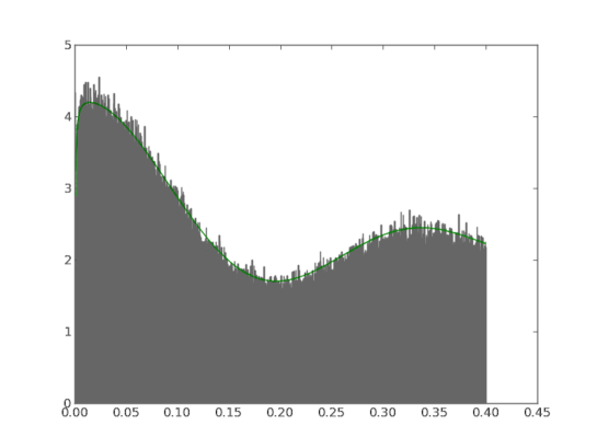
Figure 1 shows that for suitably chosen and , just using the first four residues gives an excellent approximation to the one level density.
Figure 1: One level density for the excised ensemble with , generated numerically using matrices, with the first four terms (up to ) from (158) plotted in green. Both plots are normalised to have unit area under the curve.
6A mixed moment of elliptic curve -functions
The equivalent quantity to the random matrix moment we calculated in the last section is
(161)
We will obtain an expression for this by differentiating once the ratios conjecture below, choosing to be .
In [14], Conrey, Farmer and Zirnbauer derived the following ratios conjecture. It is not stated explicitly in that paper, but is mentioned after their equation (6.31) as following from their Conjecture 5.3 and their Lemma 6.8 in analogy with (6.31). There are possibly some typos in that paper, so another resource is [32] where the conjecture is stated at Conjecture 5.1 using a slightly different set notation.
(162)
where
(163)
with
(164)
(165)
and
(166)
Here, and is a scalar and the contours of integration enclose all the ’s but avoid the singularities of .
The arithmetic factor is a product over primes which is convergent where we need to use it. It was first derived in [14] and is examined in some detail. It is stated in general at equation (5.37) in that paper (they call it ) and examined further in Section 6.3, however there are possible typos to beware of. We use the version in Mason and Snaith [32] in Conjecture 5.1 and translate here their set notation for an example
for the specific family of quadratic twists of the -function associated with the elliptic curve .
(168)
If we start using :
This has exactly the same polar structure as (2) - it behaves like the equivalent integral for . In the above we have defined to make the comparison easier. The associated with the largest in the sum, , can be thought to be equivalent to the matrix size in the random matrix version. Note that in the random matrix case we found both the leading order term and the next to leading order term in , while here, for simplicity, we shall just work with the leading order term in . Acting in analogy to the random matrix case at (2) we know that we can shrink the contours of integration onto the poles, with narrow necks connecting them. As we showed in Section 2.1, the integral will cancel on either side of the necks, leaving a sum over three circular contours for each variable. The only terms which contribute to this sum will have the residue from one evaluated at , and the rest evaluated at 0. Using this fact, and in analogy with (2.1.3), we get
(169)
where
(170)
Evaluating the integral:
(171)
We are interested in the large conductor limit, so let us scale the -variables by , and as in (2.1.3)
(172)
Keeping just the leading order term, we have:
(173)
(174)
(175)
(176)
(177)
(178)
Using these,
(179)
The integral here is very nearly with the exception of the exponential. In analogy with Section 2.1.4 we write
(180)
with
(181)
Compare this with (55). In exactly the same way as at (55) we write
We set , write as for simplicity, and differentiate this with respect to :
(198)
Here . Fortunately, when we set (note is not necessarily real), several of these terms disappear. We note that . Also .
(199)
Here, . Now let
(200)
and
so
(202)
7One level density for quadratic twists of elliptic curve -functions
In Section 5, we used both the leading order term and the next to leading order terms (in ) for the mixed moment in order to calculate the one level density over . However, to make the calculation easier, we shall only use the leading order term in this time. Let denote a zero of on the half line. For a test function , let us consider the one level density
(203)
where is a suitable test function (e.g. an even Schwartz function).
Using the argument principle, we find
(204)
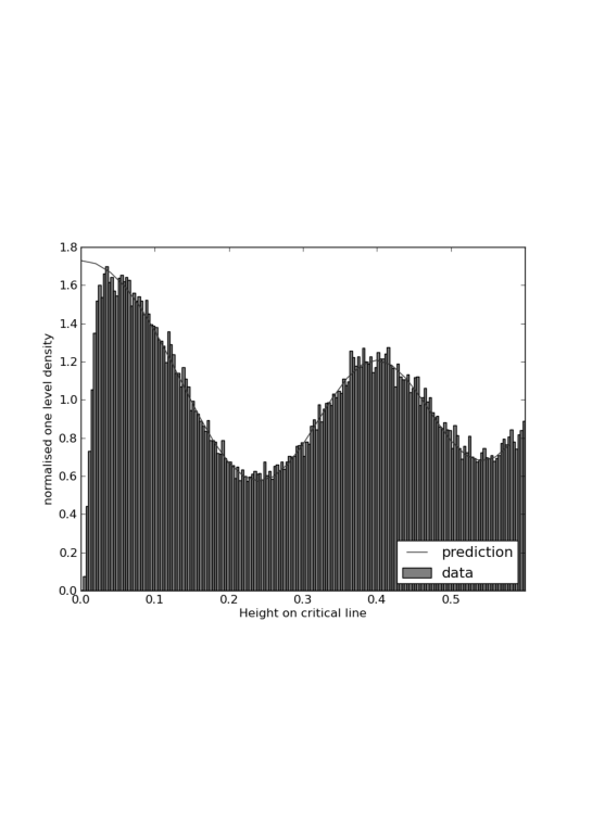
where denotes a vertical line from to , and . One can continue from here by replacing the ratio of -functions with the result of the ratios conjecture for . This was done in [25], and results in an excellent prediction for the one level density away from the critical point , but which does not capture the extra zero repulsion at the origin, as can be seen in Figure 2. Based on the work done in [20] and in [17], we believe that this extra repulsion is linked to the discretisation of the central values due to the central value formula (7). That is, the central value is either zero or it is greater than . Therefore, we might expect that if we explicitly enforce this bound using a Heaviside step function, we would get a prediction for the one level density which does contain information about the central value which might have been lost in the approximations of the ratios conjecture recipe. Therefore we define our one level density in the following way:
(205)
where . The value of has been computed for many families by Michael Rubinstein and can be found in Table 3 of [15]. Using the integral representation of the Heaviside function (144), we get
(206)
where . We can move the logarithmic derivative of inside the integral:
(207)
Let us first consider the integral over on the line. If we replace the ratios of -functions by the result in (6), the integrand no longer has poles in for on the line, so we can then move the path of integration onto to get
(208)
Here again we are assuming can be a complex variable, rather than just an integer, and from here on we will neglect error terms. Our purpose is to show that this method gives qualitatively the correct behaviour of the one level density near the origin.
For the integral, we change variables so that we can write it as an integral over :
(209)
The functional equation for these -functions looks like
(210)
where
(211)
We take the derivative of the functional equation
(212)
We then replace the ratio of -functions with the result in (6), to find that for the integral over , we get:
(213)
We know from Section 5 that has poles at the negative half-integers, and the term is the one level density already derived in [25], so we can write this as a series of residues:
(214)
7.1The term
This corresponds to the one level density derived at Theorem 2.3 in [25] (with slightly different notation for the arithmetic parts):
Figure 2: One level density of zeros for even twists with of the -function associated with the elliptic curve . We can see that the prediction due to the ratios conjecture as calculated in [25] (the smooth curve, reproduced in (7.1) here) fails to capture the behaviour of the one level density close to the origin.
7.2The contribution from higher residues
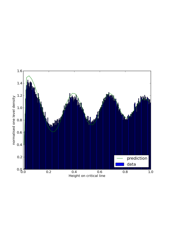
The higher residues will not take such a neat form, but may be calculated using a computational algebra package, and the resulting one level density prediction using the first three residues is shown in Figure 3. Near the origin, this is a marked improvement on the prediction using only the first residue, i.e. the prediction from [25] in Figure 2. Away from the origin, it is less good, but since we are only using the first three residues and we are only working to leading order term in , it is reasonable to suppose that if we calculated more residues and/or higher order terms in , then we would get even better agreement. This supports the hypothesis that information about the discretisation of the central values is lost in the error term of the ratios conjecture for finite conductor.
Figure 3: One level density of zeros for even twists with of the L-function associated with the elliptic curve , with the first three residues from the prediction (7).
References
[1]
S.A. Altuǧ, S. Bettin, I. Petrow, Rishikesh, and I. Whitehead.
A recursion formula for moments of derivatives of random matrix
polynomials.
Quart. J. Math., 65:1111–25, 2014.
[2]
E. Alvarez and N.C. Snaith.
Moments of the logarithmic derivative of characteristic polynomials
from and .
Journal of Mathematical Physics, 61(10), 2020.
[3]
J.C. Andrade and C.G. Best.
Joint moments of derivatives of characteristic polynomials of random
symplectic and orthogonal matrices.
J. Phys. A, 57(20), 2024.
arXiv:2312.04981.
[4]
A. Ash and R. Gross.
Curves, Counting and Number Theory.
Princeton University Press, 2012.
[5]
T. Assiotis, M.A. Gunes, J.P. Keating, and F. Wei.
Exchangeable arrays and integrable systems for characteristic
polynomials of random matrices.
arXiv:2407.19233.
[6]
T. Assiotis, M.A. Gunes, and A. Soor.
Convergence and an explicit formula for the joint moments of the
circular Jacobi -ensemble characteristic polynomial.
Math. Phys. Anal. Geom., 25(15), 2022.
[7]
T. Assiotis, J.P. Keating, and J. Warren.
On the joint moments of the characteristic polynomials of random
unitary matrices.
IMRN, 2022(18), 2022.
[8]
E.C. Bailey, S. Bettin, G. Blower, J.B. Conrey, A. Prokhorov, M.O. Rubinstein,
and N.C. Snaith.
Mixed moments of characteristic polynomials of random unitary
matrices.
J. Math. Phys., 60(8), 2019.
[9]
Y. Barhoumi-Andréani.
A new approach to the characteristic polynomial of a random unitary
matrix.
arXiv:2011.02465.
[10]
E.W. Barnes.
The theory of the -function.
Q. J. Math., 31:264–314, 1900.
[11]
E. Basor, P. Bleher, R. Buckingham, T. Grava, A. Its, E. Its, and J. Keating.
A representation of joint moments of CUE characteristic polynomials
in terms of Painlevé functions.
Nonlinearity, 32(10):4033–4078, 2019.
arXiv:1811.00064.
[12]
E. Brézin and S. Hikami.
Characteristic polynomials of random matrices.
Comm. Math. Phys., 214:111–135, 2000.
arXiv:math-ph/9910005.
[13]
J.B. Conrey, D.W. Farmer, J.P. Keating, M.O. Rubinstein, and N.C. Snaith.
Integral moments of -functions.
Proc. London Math. Soc., 91(1):33–104, 2005.
arXiv:math.nt/0206018.
[14]
J.B. Conrey, D.W. Farmer, and M.R. Zirnbauer.
Autocorrelation of ratios of -functions.
Comm. Number Theory and Physics, 2(3):593–636, 2008.
arXiv:0711.0718.
[15]
J.B. Conrey, J.P. Keating, M.O. Rubinstein, and N.C. Snaith.
Random matrix theory and the Fourier coefficients of half-integral
weight forms.
Experiment. Math., 15(1):67–82, 2006.
arXiv:math.nt/0412083.
[16]
J.B. Conrey, M.O. Rubinstein, and N.C. Snaith.
Moments of the derivative of characteristic polynomials with an
application to the Riemann zeta-function.
Comm. Math. Phys., 267(3):611–629, 2006.
arXiv:math.NT/0508378.
[17]
I. A. Cooper, Patrick W. Morris, and N.C. Snaith.
Beyond the excised ensemble: modelling elliptic curve
-functions with random matrices.
Journal of Physics A: Mathematical and Theoretical, 49(7),
2016.
[18]
P.-O. Dehaye.
Joint moments of derivatives of characteristic polynomials.
Alg. Number Theory, 2(1):31–68, 2008.
arXiv:math/0703440.
[19]
P.-O. Dehaye.
A note on moments of derivatives of characteristic polynomials.
In DMTCS Proceedings, 22nd International Conference on formal
power series and algebraic combinatorics, volume AN. Discrete mathematics
and Theoretical Computer Science, 2010.
[20]
E. Dueñez, D. K. Huynh, S. J. Miller, J. P. Keating, and N. C. Snaith.
A random matrix model for elliptic curve -functions of finite
conductor.
J. Phys. A, 45(11), 2012.
arXiv:1107.4426.
[21]
A. Fazzari.
On the joint second moment of zeta and its logarithmic derivative.
arXiv:2310.15918.
[22]
P.J. Forrester.
Joint moments of a characteristic polynomial and its derivative for
the circular -ensemble.
Probability and mathematical physics, 3(1), 2022.
[24]
C.P. Hughes.
On the characteristic polynomial of a random unitary matrix and
the Riemann zeta function.
PhD thesis, University of Bristol, 2001.
[25]
D.K. Huynh, J.P. Keating, and N.C. Snaith.
Lower order terms for the one-level density of elliptic curve
-functions.
J. Number Theory, 129:2883–2902, 2009.
arXiv:0811.2304.
[26]
N.M. Katz and P. Sarnak.
Random Matrices, Frobenius Eigenvalues and Monodromy.
American Mathematical Society Colloquium Publications, 45. American
Mathematical Society, Providence, Rhode Island, 1999.
[27]
N.M. Katz and P. Sarnak.
Zeros of zeta functions and symmetry.
Bull. Amer. Math. Soc., 36:1–26, 1999.
[28]
J.P. Keating and N.C. Snaith.
Random matrix theory and -functions at .
Comm. Math. Phys, 214:91–110, 2000.
[29]
J.P. Keating and F. Wei.
Joint moments of higher order derivatives of CUE characteristic
polynomials I: asymptotic formulae.
IMRN, 12, 2024.
arXiv:2307.01625.
[30]
J.P. Keating and F. Wei.
Joint moments of higher order derivatives of CUE characteristic
polynomials II: structures, recursive relations and applications.
Nonlinearity, 37(8), 2024.
arXiv:2307.02831.
[31]
W. Kohnen and D. Zagier.
Values of -series of modular forms at the center of the critical
strip.
Invent. Math., 64:175–198, 1981.
[32]
A.M. Mason and N.C.Snaith.
Orthogonal and symplectic -level densities.
Memoirs of the AMS, 251(1194), 2018.
arXiv:1509.05250.
[33]
E. Moshe Baruch and Z. Mao.
Central values of automorphic -functions.
Geom. Func. Anal., 17:333–384, 2007.
[34]
K. Rubin and A. Silverberg.
Ranks of elliptic curves.
Bull. Amer. Math. Soc., 39(4):455–74, 2002.
[35]
N. Simm and F. Wei.
Private communication.
[36]
J.-L. Waldspurger.
Sur les coefficients de Fourier des formes modulaires de poids
demi-entier.
J. Math. Pures Appl., 60(9):375–484, 1981.
[37]
B. Winn.
Derivative moments for characteristic polynomials from the CUE.
Commun. Math. Phys., 315:531–562, 2012.