Application of Langevin Dynamics to Advance the Quantum Natural Gradient Optimization Algorithm

Abstract

A Quantum Natural Gradient (QNG) algorithm for optimization of variational quantum circuits has been proposed recently. In this study, we employ the Langevin equation with a QNG stochastic force to demonstrate that its discrete-time solution gives a generalized form of the above-specified algorithm, which we call Momentum-QNG. Similar to other optimization algorithms with the momentum term, such as the Stochastic Gradient Descent with momentum, RMSProp with momentum and Adam, Momentum-QNG is more effective to escape local minima and plateaus in the variational parameter space and, therefore, achieves a better convergence behavior compared to the basic QNG. Our open-source code is available at https://github.com/borbysh/Momentum-QNG

1 Introduction

Optimization of variational quantum circuits in hybrid quantum-classical algorithms has become a popular task over the recent time. The best known applications include the Variational Quantum Eigensolver (VQE) [1], Quantum Approximate Optimization Algorithm (QAOA) [2] and Quantum Neural Networks (QNNs) [3, 4, 5].

A computationally efficient method for evaluating analytic gradients on quantum hardware has been recently proposed [6]. Therefore, the application of optimization algorithms from the Stochastic Gradient Descent (SGD) family has become possible. However, the path of steepest descent in the parameter space, guided by the (opposite) gradient vector direction, is usually not optimal, because it depends on the number of variational parameters, which is usually excessive. The same overparametrization problem is present in classical Machine Learning (ML) (see, e.g., [7]). To mitigate it, a Natural Gradient (NG) concept has been proposed [8]. Contrary to vanilla SGD, NG determines the steepest descent direction taking into account the Riemannian metric tensor. In this way, the optimization path becomes invariant under arbitrary reparametrization (see [8]) and, therefore, does not suffer from overparametrization [9].

Inspired by the NG approach, Stokes et al. [10] have recently proposed its generalization to the quantum circuit optimization task, which they called a Quantum Natural Gradient (QNG) optimizer. They considered a parametric family of unitary operators $U_{\theta}\in U(N)$, which are indexed by real parameters $\theta\in\mathbb{R}^{d}$. With a fixed reference unit vector $|0\rangle\in\mathbb{C}^{N}$ and a Hermitian operator $H=H^{\dagger}$ acting on $\mathbb{C}^{N}$, they consider the following optimization problem

$$\min_{\theta\in\mathbb{R}^{d}}\mathcal{L}(\theta)\,,\quad\mathcal{L}(\theta)=\frac{1}{2}\operatorname{tr}(P_{\psi_{\theta}}H)=\frac{1}{2}\langle\psi_{\theta},H\psi_{\theta}\rangle\,,$$ (1)

where $\psi_{\theta}=U_{\theta}|0\rangle$ and $P_{\psi_{\theta}}\in\mathbb{CP}^{N-1}$ is the associated projector. Note that $\psi_{\theta}$ is normalized, since $U_{\theta}$ is unitary. Any local optimum of the nonconvex objective function $\mathcal{L}(\theta)$ can be found by iterating the following discrete-time dynamical system,

$$\theta_{n+1}=\operatorname*{arg\,min}_{\theta\in\mathbb{R}^{d}}\left[\langle\theta-\theta_{n},\nabla\mathcal{L}(\theta_{n})\rangle\phantom{\frac{1}{2\eta}}\right.$$

$$\left.+\frac{1}{2\eta}\|\theta-\theta_{n}\|_{g(\theta_{n})}^{2}\right]\,,$$ (2)

where $\eta>0$ is a positively defined constant, $g(\theta_{n})$ is the symmetric matrix of the Fubini-Study metric tensor $g_{ij}(\theta)=\operatorname{Re}[G_{ij}(\theta)]$, and the Quantum Geometric Tensor is defined as follows (for further details see [10] and references therein):

$$G_{ij}(\theta)=\left\langle\frac{\partial\psi_{\theta}}{\partial\theta^{i}},\frac{\partial\psi_{\theta}}{\partial\theta^{j}}\right\rangle-\left\langle\frac{\partial\psi_{\theta}}{\partial\theta^{i}},\psi_{\theta}\right\rangle\left\langle\psi_{\theta},\frac{\partial\psi_{\theta}}{\partial\theta^{j}}\right\rangle\,.$$ (3)

In (1), according to [10], we introduced the following notation:

$$\|\theta-\theta_{n}\|_{g(\theta_{n})}^{2}=\langle\theta-\theta_{n},g(\theta_{n})(\theta-\theta_{n})\rangle\enspace.$$ (4)

Then, the first-order optimality condition corresponding to (1) is:

$$g(\theta_{n})(\theta_{n+1}-\theta_{n})=-\eta\cdot\nabla\mathcal{L}(\theta_{n})\enspace.$$ (5)

A solution of the optimization problem (1) is thus provided by the following expression which involves the inverse $g^{-1}(\theta_{n})$ of the metric tensor:

$$\theta_{n+1}-\theta_{n}=-\eta\cdot g^{-1}({\theta_{n}})\nabla\mathcal{L}(\theta_{n})\enspace.$$ (6)

In this way, with the Fubini-Study metric tensor introduced, the implied descent direction in the parameter space, given by the right-hand side of (6), becomes invariant with respect to arbitrary reparametrization and, therefore, to the details of QNN architecture. With their QNG optimizer (6), the authors of [10] achieved a considerable optimization performance improvement as compared with SGD and Adam [11].

However, being rather effective for convex optimization, QNG often sticks to local minima, saddles and plateaus of non-convex loss functions. In classical ML applications, employing optimization algorithms with momentum (inertial) term, such as SGD with momentum [12], RMSProp with momentum [13] and Adam [11], has demonstrated better convergence characteristics.

Recently, Borysenko and Byshkin [14] demonstrated that a discrete-time solution of the Langevin equation with stochastic gradient force term results into the well-known SGD with momentum [12] optimization algorithm. In this paper, we consider the Langevin equation with the QNG stochastic force term. In Section 2 we show that its discrete-time solution yields a generalized QNG optimization algorithm, which we call Momentum-QNG. In Section 3 we benchmark it together with the basic QNG, Momentum and Adam on several optimization tasks to demonstrate its enhanced performance.

2 Langevin equation with QNG force

The adaptation of Langevin dynanimcs for optimization suggests a new prospective research direction (see, e.g., [15] and [16] ). For optimization of analitically defined objective functions, even a quantum form of the Langevin dynamics has been proposed [17]. In Langevin dynamics, two forces are added to the classical Newton equation of motion – a viscous friction force proportional to the velocity with a friction coefficient $\gamma\geq 0$ and a thermal white noise. Explicitly, the Langevin dynamics of a (Brownian) particle with unit mass $m=1$ in the space of real variables $\theta\in\mathbb{R}^{d}$ and real time $t$ can be described by the following equation (see e.g. [18, 19, 20, 21]):

$$\frac{dv(t)}{dt}=f(\theta)-\gamma v(t)+R(t),$$ (7)

where $v=d\theta/dt$ denotes velocities and $R(t)$ is a random uncorrelated force with zero mean.

The discrete-time form of (7) with stochastic force $\hat{f}=f+R$ reads:

$$\frac{\Delta\theta_{n+1}-\Delta\theta_{n}}{\Delta t^{2}}=\hat{f}_{n}-\gamma\frac{\Delta\theta_{n+1}+\Delta\theta_{n}}{2\Delta t},$$ (8)

where $\Delta\theta_{n+1}=\theta_{n+1}-\theta_{n}$ and $\Delta t$ is a time step. Now, it is straightforward to obtain the next parameter updating formula:

$$\Delta\theta_{n+1}=\rho\Delta\theta_{n}+\hat{f}_{n}\cdot\eta$$ (9)

with

$$\rho=\frac{1-\gamma\Delta t/2}{1+\gamma\Delta t/2}$$ (10)

and

$$\eta=\frac{\Delta t^{2}}{1+\gamma\Delta t/2}=\frac{1+\rho}{2}\Delta t^{2}.$$ (11)

Equation (9) is nothing else but a well-known SGD with momentum optimization algorithm [12] (further referred to as Momentum) with $\rho$ being a momentum coefficient and $\eta$ a learning rate constant.

Setting

$$\hat{f}_{n}=-g^{-1}({\theta_{n}})\nabla\mathcal{L}(\theta_{n}),$$ (12)

from (9) one obtains a generalized form of (6):

$$\Delta\theta_{n+1}=\rho\Delta\theta_{n}-\eta\cdot g^{-1}({\theta_{n}})\nabla\mathcal{L}(\theta_{n}),$$ (13)

which we call Momentum-QNG. Note, that (13) reduces to (6) for $\rho=0$.

From (13) one can see that our Momentum-QNG optimization algorithm is a quantum adaptation of SGD with momentum [12] and should not be confused with the recently introduced Momentum QNG algorithm [22] (which is a quantum adaptation of Adam [11]) proposed by the authors of qBang [22].

3 Results and discussion

In this section we benchmark Momentum-QNG with reference to other gradient-based algorithms, such as basic QNG, Adam and Momentum optimizers. In all calculations we set $\Delta\theta_{0}=0$ as the initial condition.

3.1 Variational Quantum Eigensolvers

Our first test-drive model is an Investment Portfolio Optimization task treated with the VQE approach. To compare the performance of different optimizers, we run a series of 200 trials on a modified tutorial code [23]. Each trial is initialized with the random-guess values of variational parameters, being the same for all optimizers. Next, the optimization process runs for 200 steps or until energy convergence up to the 3-digit accuracy. The values of hyperparameters are as follows: $0.01\leq\eta\leq 0.25$, $\rho=0.9$ for Momentum and Momentum-QNG, and $\beta_{1}=0.9$, $\beta_{2}=0.99$, $\epsilon=10^{-8}$ for Adam. To compare the performance of different optimizers, we calculate the mean and standard deviation values of $\Delta E=E_{opt}-E_{ground}$ – the difference between the optimized and the ground state energy. From Fig. 1(a) one can see that Momentum-QNG gives the least mean $\Delta E$ between all the optimizers studied over the whole range of stepsize (learning rate $\eta$) values under consideration.

To study the convergence behaviour of the optimization algorithms under consideration, in Fig. 1(b) we plot the mean (symbols) and the standard deviation (error bars) of the number of steps to convergence of the optimization procedure in a series of 200 trials, as a function of the stepsize value (learning rate, $\eta$). One can see that Momentum-QNG demonstrates a decent convergence behavior over the whole range of stepsize values under consideration and even the best one for $\eta\leq 0.075$. For further details of our calculations see [24].

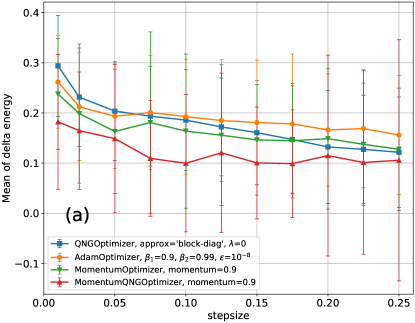
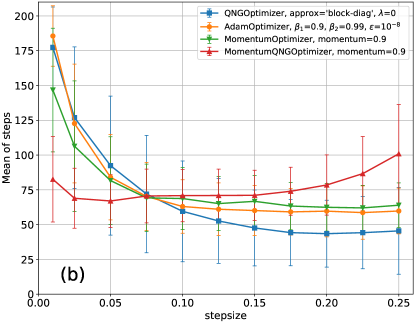
Figure 1: Benchmarking Momentum-QNG together with QNG, Momentum and Adam on the portfolio optimization problem. The vertical axis shows the mean (symbols) and the standard deviation (error bars) of the difference between the optimized and the ground state energy (a) and the number of steps to convergence (b) in a series of 200 trials, while the horizontal axis shows the stepsize value (learning rate, $\eta$) of four different optimizers under consideration. Each trial is initialized with random-guess values of the variational parameters, being the same for all optimizers. Then the optimization process runs for 200 steps (or until convergence) independently by each optimizer.

3.2 Quantum Approximate Optimization Algorithm

Our second test model is the Minimum Vertex Cover problem treated with the QAOA approach. Recently, this problem has been used to study the impact of noise on classical optimizers and to determine the optimal depth of the QAOA circuit [25]. In our calculations we use a modified code by Jack Ceroni [26] for the 4-qubit Minimum Vertex Cover problem. For this problem we run a series of 200 trials with the same for all optimizers random-guessed initial values of variational parameters. The optimization process runs for 200 steps or until energy convergence up to the 2-digit accuracy during at least 6 steps. To compare the performance of different optimizers, we calculate the quality ratio of the final optimized state - the total probability to find the states of the exact solution in the given optimized solution. The values of hyperparameters are as follows: $0.01\leq\eta\leq 0.25$, $\rho=0.9$ for Momentum and Momentum-QNG, and $\beta_{1}=0.9$, $\beta_{2}=0.99$, $\epsilon=10^{-8}$ for Adam. From Fig. 2(a) one can see that in the range of stepsize (learning rate $\eta$) values under consideration Adam, Momentum and Momentum-QNG achieve almost equal maximal values of the quality ratio. At the same time we note that, for $\eta<0.2$, Momentum-QNG systematically outperforms both Adam and original QNG.

To study the convergence behaviour of the optimization algorithms under consideration, on Fig. 2(b) we plot the mean (symbols) and the standard deviation (error bars) of the number of steps to convergence of the optimization procedure in a series of 200 trials, as a function of the value of stepsize (learning rate, $\eta$). One can see that, with the increase of stepsize, Momentum quickly goes above the convergence limit, QNG and Momentum-QNG demonstrate the intermediate results, while Adam shows the best convergence behaviour. For further details of our calculations see [27].

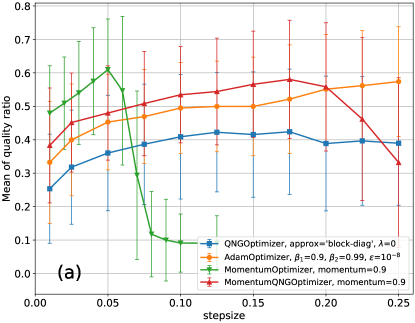
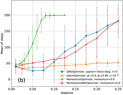
Figure 2: Benchmarking Momentum-QNG together with QNG, Momentum and Adam on the Minimum Vertex Cover problem. The vertical axis shows the mean (symbols) and the standard deviation (error bars) of the quality ratio (a) and of the number of steps to convergence (b) in a series of 200 trials, while the horizontal axis shows the value of stepsize (learning rate, $\eta$) of four different optimizers under consideration. Each trial is initialized with random-guess values of the variational parameters, being the same for all optimizers. Then the optimization process runs for 200 steps (or until convergence) independently by each optimizer.

4 Conclusions

In this paper we demonstrate that application of Langevin dynamics with Quantum Natural Gradient force for optimization of variational quantum circuits gives a new optimization algorithm, which we call Momentum-QNG. The basic QNG algorithm uses the metric tensor to rescale the variational parameter space to give a more symmetric shape of the loss function to smooth the optimization path. On the other hand, the momentum (inertial) term in the Momentum algorithm prevents the optimization process from sticking to the local minima and plateaus. Here we report that the combination of both these features in the Momentum-QNG algorithm gives a strong boost effect. Indeed, for the Minimum Vertex Cover problem (see Fig. 2(a)) the proposed Momentum-QNG algorithm outperforms the basic QNG for the same values of the learning rate $\eta<0.25$. And for the Investment Portfolio Optimization problem (see Fig. 1(a)) it gives the best result between all the optimizers under consideration. At the same time we note that when there are no loss function barriers and plateaus separating the initial and the desired optimized state of the system, one should set $\rho=0$ in the Momentum-QNG algorithm (or simply use the basic QNG one) to reduce the number of steps to convergence.

Appendix A Cumulative probability distributions

In this appendix section we present the cumulative probability distributions calculated for different stepsize values.

A.1 Investment Portfolio Optimization problem

From Fig. 3 one can see that Momentum-QNG gives the highest probability to find the energy of the final optimized state within the range $\Delta E\leq 0.2$. At the same time from Fig. 4 one can see that Momentum-QNG demonstrates the least variation of the number of steps to convergence in the whole stepsize range (see also Fig. 1(b)).

A.2 Minimum Vertex Cover problem

From Fig. 5 one can see that Momentum-QNG demonstrates one of the best quality ratio distributions among the algorithms studied and definitely outperforms the basic QNG optimizer. At the same time, from Fig. 6 one can see that Momentum-QNG demonstrates a modest convergence behaviour compared to Adam, similar to the basic QNG and Momentum.

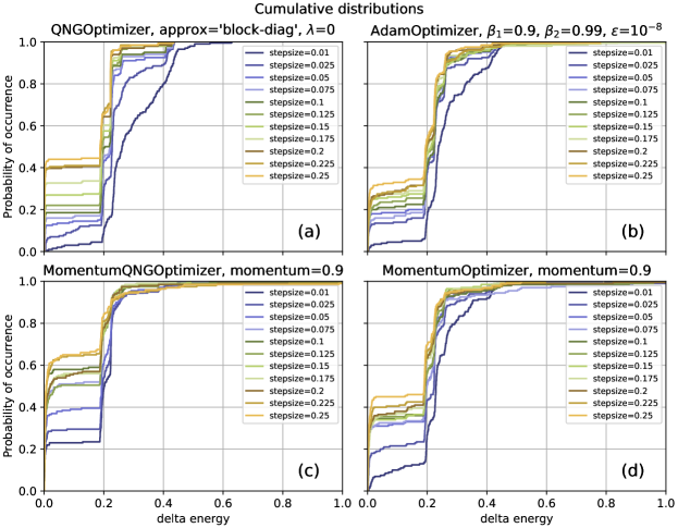
Figure 3: Benchmarking Momentum-QNG (c) together with QNG (a), Momentum (d) and Adam (b) on the Portfolio Optimization problem. The horizontal axis shows the value of the difference between the optimized and the ground state energy, while the vertical axis shows the cumulative probability to obtain the corresponding energy difference in a series of 200 trials. The curves are calculated for all values of the stepsize (learning rate, $\eta$) under consideration.

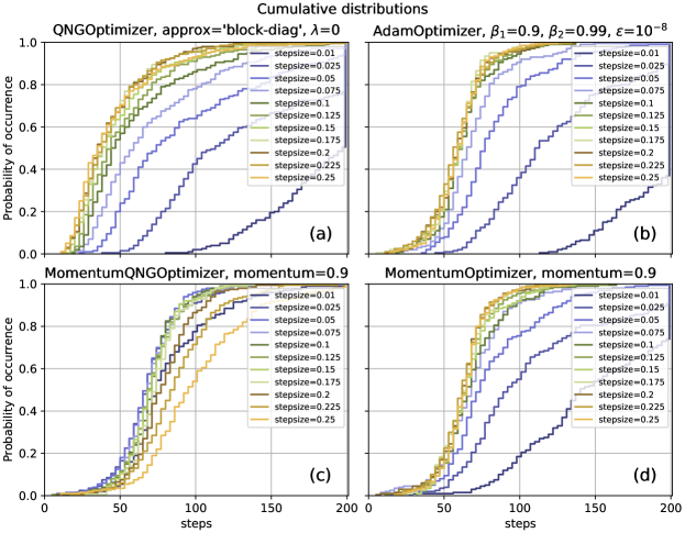
Figure 4: Benchmarking Momentum-QNG (c) together with QNG (a), Momentum (d) and Adam (b) on the Portfolio Optimization problem. The horizontal axis shows the number of steps to energy convergence up to the 3-digit accuracy, while the vertical axis shows the cumulative probability to obtain the corresponding number of steps in a series of 200 trials. The curves are calculated for all values of the stepsize (learning rate, $\eta$) under consideration.

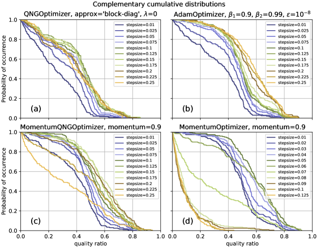
Figure 5: Benchmarking Momentum-QNG (c) together with QNG (a), Momentum (d) and Adam (b) on the Minimum Vertex Cover problem. The horizontal axis shows the value of the quality ratio, being a characteristic of an optimized state, while the vertical axis shows the cumulative probability to obtain the corresponding quality ratio in a series of 200 trials. The curves are calculated for all values of the stepsize (learning rate, $\eta$) under consideration.

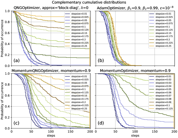
Figure 6: Benchmarking Momentum-QNG (c) together with QNG (a), Momentum (d) and Adam (b) on the Minimum Vertex Cover problem. The horizontal axis shows the number of steps to energy convergence up to the 2-digit accuracy during at least 6 steps, while the vertical axis shows the cumulative probability to obtain the corresponding number of steps in a series of 200 trials. The curves are calculated for all values of the stepsize (learning rate, $\eta$) under consideration.

References

- [1] Alberto Peruzzo, Jarrod McClean, Peter Shadbolt, Man-Hong Yung, Xiao-Qi Zhou, Peter J Love, Alán Aspuru-Guzik, and Jeremy L O’Brien. “A variational eigenvalue solver on a photonic quantum processor.”. Nature Communications 5, 4213 (2014).
- [2] Edward Farhi, Jeffrey Goldstone, and Sam Gutmann. “A quantum approximate optimization algorithm” (2014). arXiv:1411.4028.
- [3] Edward Farhi and Hartmut Neven. “Classification with quantum neural networks on near term processors” (2018). arXiv:1802.06002.
- [4] William Huggins, Piyush Patil, Bradley Mitchell, K Birgitta Whaley, and E Miles Stoudenmire. “Towards quantum machine learning with tensor networks”. Quantum Science and Technology 4, 024001 (2019).
- [5] Maria Schuld, Alex Bocharov, Krysta M. Svore, and Nathan Wiebe. “Circuit-centric quantum classifiers”. Physical Review A101 (2020).
- [6] Maria Schuld, Ville Bergholm, Christian Gogolin, Josh Izaac, and Nathan Killoran. “Evaluating analytic gradients on quantum hardware”. Phys. Rev. A 99, 032331 (2019).
- [7] Behnam Neyshabur, Russ R Salakhutdinov, and Nati Srebro. “Path-sgd: Path-normalized optimization in deep neural networks”. In C. Cortes, N. Lawrence, D. Lee, M. Sugiyama, and R. Garnett, editors, Advances in Neural Information Processing Systems. Volume 28. Curran Associates, Inc. (2015). url: https://proceedings.neurips.cc/paper_files/paper/2015/file/eaa32c96f620053cf442ad32258076b9-Paper.pdf.
- [8] Shun-ichi Amari. “Natural Gradient Works Efficiently in Learning”. Neural Computation 10, 251–276 (1998).
- [9] Tengyuan Liang, Tomaso Poggio, Alexander Rakhlin, and James Stokes. “Fisher-Rao metric, geometry, and complexity of neural networks”. In Kamalika Chaudhuri and Masashi Sugiyama, editors, Proceedings of the Twenty-Second International Conference on Artificial Intelligence and Statistics. Volume 89 of Proceedings of Machine Learning Research, pages 888–896. PMLR (2019). url: http://proceedings.mlr.press/v89/liang19a/liang19a.pdf.
- [10] James Stokes, Josh Izaac, Nathan Killoran, and Giuseppe Carleo. “Quantum natural gradient”. Quantum 4, 269 (2020).
- [11] Diederik P. Kingma and Jimmy Ba. “Adam: A method for stochastic optimization” (2014). arXiv:1412.6980.
- [12] D. Rumelhart, G. Hinton, and R. Williams. “Learning representations by back-propagating errors.”. Nature 323, 533–536 (1986).
- [13] Tijmen Tieleman and Geoffrey Hinton. “Lecture 6e rmsprop: Divide the gradient by a running average of its recent magnitude”. COURSERA: Neural networks for machine learning 4, 26–31 (2012). url: https://www.cs.toronto.edu/~tijmen/csc321/slides/lecture_slides_lec6.pdf.
- [14] O. Borysenko and M. Byshkin. “Coolmomentum: a method for stochastic optimization by Langevin dynamics with simulated annealing.”. Sci Rep 11, 10705 (2021).
- [15] Nanyang Ye, Zhanxing Zhu, and Rafal Mantiuk. “Langevin dynamics with continuous tempering for training deep neural networks”. In Advances in Neural Information Processing Systems. Pages 618–626. (2017). url: https://proceedings.neurips.cc/paper_files/paper/2017/file/019d385eb67632a7e958e23f24bd07d7-Paper.pdf.
- [16] Yi-An Ma, Yuansi Chen, Chi Jin, Nicolas Flammarion, and Michael I Jordan. “Sampling can be faster than optimization”. Proceedings of the National Academy of Sciences 116, 20881–20885 (2019).
- [17] Zherui Chen, Yuchen Lu, Hao Wang, Yizhou Liu, and Tongyang Li. “Quantum Langevin Dynamics for Optimization” (2024). arXiv:2311.15587v2.
- [18] Giovanni Bussi and Michele Parrinello. “Accurate sampling using Langevin dynamics”. Physical Review E 75, 056707 (2007).
- [19] Eric Vanden-Eijnden and Giovanni Ciccotti. “Second-order integrators for Langevin equations with holonomic constraints”. Chemical Physics Letters 429, 310–316 (2006).
- [20] W.F. Van Gunsteren and H.J.C. Berendsen. “Algorithms for Brownian dynamics”. Molecular Physics 45, 637–647 (1982).
- [21] Tamar Schlick. “Molecular modeling and simulation: an interdisciplinary guide”. Volume 21 of Interdisciplinary Applied Mathematics. Springer Verlag. (2010). url: https://link.springer.com/book/10.1007/978-1-4419-6351-2.
- [22] David Fitzek, Robert S. Jonsson, Werner Dobrautz, and Christian Schäfer. “Optimizing Variational Quantum Algorithms with qBang: Efficiently Interweaving Metric and Momentum to Navigate Flat Energy Landscapes”. Quantum 8, 1313 (2024).
- [23] Chi-Chun Chen. https://eric08000800.medium.com/portfolio-optimization-with-variational-quantum-eigensolver-vqe-2-477a0ee4e988 (2023).
- [24] Oleksandr Borysenko, Mykhailo Bratchenko, Ilya Lukin, Mykola Luhanko, Ihor Omelchenko, Andrii Sotnikov, and Alessandro Lomi. https://github.com/borbysh/Momentum-QNG/blob/main/portfolio_optimization.ipynb (2024).
- [25] Aidan Pellow-Jarman, Shane McFarthing, Ilya Sinayskiy, Daniel K Park, Anban Pillay, and Francesco Petruccione. “The effect of classical optimizers and ansatz depth on QAOA performance in noisy devices”. Scientific Reports 14, 16011 (2024).
- [26] Jack Ceroni. “Intro to QAOA”. https://pennylane.ai/qml/demos/tutorial_qaoa_intro/ (2024).
- [27] Oleksandr Borysenko, Mykhailo Bratchenko, Ilya Lukin, Mykola Luhanko, Ihor Omelchenko, Andrii Sotnikov, and Alessandro Lomi. https://github.com/borbysh/Momentum-QNG/blob/main/QAOA_depth4.ipynb (2024).