Counterfactual Fairness by Combining Factual and Counterfactual Predictions
Abstract
In high-stake domains such as healthcare and hiring, the role of machine learning (ML) in decision-making raises significant fairness concerns. This work focuses on Counterfactual Fairness (CF), which posits that an ML model’s outcome on any individual should remain unchanged if they had belonged to a different demographic group. Previous works have proposed methods that guarantee CF. Notwithstanding, their effects on the model’s predictive performance remains largely unclear. To fill in this gap, we provide a theoretical study on the inherent trade-off between CF and predictive performance in a model-agnostic manner. We first propose a simple but effective method to cast an optimal but potentially unfair predictor into a fair one without losing the optimality. By analyzing its excess risk in order to achieve CF, we quantify this inherent trade-off. Further analysis on our method’s performance with access to only incomplete causal knowledge is also conducted. Built upon it, we propose a performant algorithm that can be applied in such scenarios. Experiments on both synthetic and semi-synthetic datasets demonstrate the validity of our analysis and methods.
1 Introduction
Machine learning (ML) has been widely used in high-stake domains such as healthcare (Daneshjou et al., 2021), hiring (Hoffman et al., 2018), criminal justice (Brennan et al., 2009), and loan assessment (Khandani et al., 2010), bringing with it critical ethical and social considerations. A prominent example is the bias observed in the COMPAS tool against African Americans in recidivism predictions (Brackey, 2019). This issue is particularly alarming in an era where large-scale deep learning models, commonly trained on noisy data from the internet, are increasingly prevalent. Such models, due to their extensive reach and impact, amplify the potential for widespread and systemic biases. This increasing awareness underscores the need for ML practitioners to integrate fairness considerations into their work, extending their focus beyond merely maximizing prediction accuracy (Bolukbasi et al., 2016; Calders and Verwer, 2010; Dwork et al., 2012; Grgic-Hlaca et al., 2016; Hardt et al., 2016). Various fairness notions have been developed, ranging from group-level measures such as group parity (Hardt et al., 2016) to individual-level metrics (Dwork et al., 2012). Recently, there has been a growing interest in approaches based on causal inference, particularly in understanding the causal effects of sensitive attributes such as gender and age on decision-making (Chiappa, 2019; Galhotra et al., 2022; Khademi et al., 2019). This has led to the proposal of Counterfactual Fairness (CF), which states that prediction for an individual in hypothetical scenarios where their sensitive attributes differ should remain unchanged (Kusner et al., 2017). As an individual-level notion agnostic to the choice of similarity measure (Kusner et al., 2017; Rosenblatt and Witter, 2023a), CF has recently gained traction (Anthis and Veitch, 2024; Nilforoshan et al., 2022; Makhlouf et al., 2022; Rosenblatt and Witter, 2023b).
To achieve CF, Kusner et al. (2017) first proposed a naive solution, suggesting that predictions should only use non-descendants of the sensitive attribute in a causal graph. This approach only requires a causal topological ordering of variables and achieves perfect CF by construction. However, it limits the available features for downstream tasks and could be inapplicable in certain cases (Kusner et al., 2017). For relaxation, they further proposed an algorithm that leverages latent variables. Extending this line of work, Zuo et al. (2023) introduced a technique that incorporates additional information by mixing factual and counterfactual samples. Although perfect CF has been established in their work, its predictiveness degraded, and whether the predictive power can be improved remains unknown. In parallel to this, another branch of research employed regularization and augmentation to encourage CF (Garg et al., 2019; Stefano et al., 2020; Kim et al., 2021). However, as these methods cannot guarantee perfect CF, analyzing the optimal predictive performance under CF constraints is highly challenging.
To take a first step in understanding this problem, we conduct a formal quantitative study on the inherent trade-off between Counterfactual Fairness (CF) and predictive performance, which quantifies the predictive power that has to be given up for satisfying the fairness (i.e., perfect CF) criteria(Zhao and Gordon, 2022; Xian et al., 2023). Towards this goal, we first prove that the optimal predictor under the fairness constraint can be achieved by combining factual and counterfactual predictions using a (potentially unfair) optimal predictor. To the best of our knowledge, this is the first counterfactually fair predictor that is proven optimal. Next, we quantify the excess risk between the optimal predictor with and without CF constraints. This quantity sheds lights on the best possible model, in terms of predictive performance, under the stringent notion of perfect CF. To take scenarios with incomplete causal knowledge (e.g. unknown causal graph or model) in consideration, we further study the CF and predictive performance degradation caused by imperfect counterfactual estimations. Inspired by our theoretical findings, we first propose a plugin method that leverages a (potentially unfair) pretrained model to achieve optimal fair prediction and further propose a practical way to achieve good empirical performance under counterfactual estimation inaccuracies.
We summarize our contributions as follows:
-
1.
To the best of our knowledge, we propose the first CF method that is provably optimal in terms of predictive performance under perfect CF and characterize their inherent trade-off, which applies to all CF methods.
-
2.
We investigate the CF and predictive performance degradation from estimation error resulting from limited causal knowledge and propose methods to mitigate estimation errors in practice.
-
3.
We empirically demonstrate that our proposed CF methods outperform existing methods in both the full and incomplete causal knowledge settings.
2 Preliminaries
2.1 Notation
We use capital letter to represent random variables and lowercase letters to represent the realization of random variables. Now we define a few variables that will be considered in this work. represents the sensitive attribute of an individual (e.g. gender), represents the target variable to predict, represents observed features other than and , and represents unobserved confounding variables which are not caused by any observed variables while represent their realization respectively.
2.2 Counterfactual
In this work, we use the framework of Structrual Causal Models (SCMs) (Pearl, 2009). A SCM is a triplet where represent exogenous variables (factors outside the model), represent endogenous variables, and contains a set of functions that maps from and to .
A counterfactual query asks a question like: what would the value of be if had taken a different value given certain observations . For example, given that a person is a woman and given everything we observe about her performance in an interview, what is the probability of her getting the job if she had been a man? More formally, given a SCM, a counterfactual query can be written as . Here is the evidence and in the subscript represents the intervention on . For the general procedure to estimate counterfactual, please refer to Pearl (2009).
2.3 Counterfactual Fairness
Built upon the framework above, we focus on Counterfactaul Fairness (CF), which requires the predictors to be fair among factual and counterfactual samples. More formally, it is defined as below
Definition 2.1.
(Counterfactual Fairness) We say a predictor is counterfactually fair if
This definition states that intervention on should not affect the distribution of . Using the same example above, the probability of a woman getting the job should be the same as that if she had been a man. For that goal, we use the following metric to evaluate CF
Definition 2.2.
(Total Effect) The Total Effect (TE) of a predictor is
Therefore, a predictor is counterfactually fair if and only if . Throughout the paper, we use TE to quantify the violation of counterfactual fairness.
3 Counterfactual Fairness via Output Combination
3.1 Problem Setup
We assume that all data we have is generated by a causal model (Pearl, 2009) and we consider the representative causal graph shown in Figure 1 that has been widely adopted in the literature (Grari et al., 2023; Kusner et al., 2017; Zuo et al., 2023) For simplicity, we omit the exogenous noise variables corresponding to and in the graph. Our analysis is presented based on binary given its pivotal importance in the literature (Pessach and Shmueli, 2023) and for the sake of presentation clearness, but our analysis and our method can be naturally extended on multi-class . We first state the main assumptions needed in this section.
Assumption 3.1.
-
1.
and are independent of each other.
-
2.
The mapping between and is invertible given .
While the invertibility assumption might be restrictive in certain scenarios, it simplifies the theoretical analysis and has been adopted in recent works on counterfactual estimation (Nasr-Esfahany et al., 2023; Zhou et al., 2024). Further, we empirically validate the effectiveness of our method after relaxing this assumption in the experiment section. To facilitate our discussion, we first define as the mapping between and , i.e., . According to our second assumption, is an invertible function, i.e., . This assumption simplifies the counterfactual estimation of for different values of into a deterministic function. In our context, counterfactual estimation specifically refers to the estimation of . We introduce the concept of the counterfactual generating mechanism (CGM), denoted as . All proof can be found in Appendix A.
Given the setup, the following lemma characterizes the perfect CF constraint on .
Lemma 3.2.
Given Assumption 3.1, predictor on is counterfactually fair if and only if the predictor returns the same value for a sample and its counterfactuals, i.e.,
The proof is straightforward from the definition of TE. Notably, this lemma helps disambiguate the question whether counterfactual fairness is a distribution- or individual-level requirements as raised in Plecko and Bareinboim (2022). In our setup, they are equivalent due to invertibility between and given .
3.2 Optimal Counterfactual Fairness and Inherent Trade-off
Given the complete knowledge of the causal model, it is viable to satisfy the perfect CF constraint (Kusner et al., 2017; Zuo et al., 2023). These methods are known to result in empirical degradation of ML models performance, raising critical concerns about the fairness-utility trade-offs. However, it is still unknown to what extent the ML model performance has to be affected in order to achieve perfect CF. In this section we provide a formal study on this to close the gap.
Our solution consists of two steps. First, we propose a simple yet effective method that is provably optimal under the constraint of perfect CF. Next, we characterize the inherent trade-off between CF and predictive performance by checking the excess risk of this Bayes optimal predictor. Our result shows that the inherent trade-off is dominated by the dependency between and , echoing with previous analysis on non-causal based fairness notions (Chzhen et al., 2020; Xian et al., 2023). For brevity, we refer to a Bayes optimal predictor as “optimal”, and a model that satisfies perfect CF as “fair”.
We start with the following theorem instantiating an optimal and fair predictor.
Theorem 3.3.
Given Assumption 3.1 111Note that while the discussion in this paper focuses on the causal model in Figure 1, our theorem is valid for more general cases that satisfy Assumption 3.1. And for brevity, the following discussion is done under this assumption unless otherwise stated. and loss (i.e., squared loss for regression tasks, and cross-entropy loss for classification tasks), an optimal and fair predictor (i.e., the best possible model(s) under the constraint of perfect CF) is given by the average of the optimal (potentially unfair) predictions on itself and all possible counterfactuals:
where is the counterfactual of when intervening with , and is an unconstrained optimal predictor, i.e., .
This result suggests that, if we have to access to ground truth counterfactuals, a simple algorithm using an (potentially) unfair model could achieve strong fairness and accuracy. Remarkably, to our best knowledge, this is the first predictor that proves to achieve the optimality while being fair. Built upon the above result, we are ready to characterize the inherent trade-off between CF and model performance by the following theorem.
Theorem 3.4.
The inherent trade-off between CF and predictive performance, characterized by the excess risk of the Bayes optimal predictor under the CF constraint, is given by
for regression tasks using squared loss where denotes the variance of ; and
for classification tasks using cross-entropy loss.
Remarkably, the excess risks are completely characterized by the inherent dependency between and as determined by the underlying causal mechanism, similar to non-causal based group fairness (Chzhen et al., 2020; Xian et al., 2023). Moreover, they lower bound the excess risk of all possible predictors one may apply in order to achieve perfect CF.
3.3 Method with Incomplete Causal Knowledge
In this section, we aim at addressing CF in the scenario where causal knowledge is limited. Inspired by Theorem 3.3, we first present a simple plugin method as summarized in Algorithm 1.
For regression tasks, is the final output, and for classification tasks, is equivalent to the probability of , i.e., . It is note worthy that PCF is agnostic to the training of predictor that can be determined by the user freely. In fact, with access to the oracle CGM , then PCF would achieve perfect CF as proved in the next result.
Proposition 3.5.
Given that is the ground truth counterfactual generating mechanism, i.e., , Algorithm 1 achieves perfect CF for any pretrained predictor .
Note that the this proposition only requires access to ground truth and holds valid for any pretrained predictor . If is further accurate, then the corresponding PCF is able to achieve high accuracy as well, which is empirically validated in the experiments.
3.3.1 Given estimated
Acquiring counterfactuals in practice can be a challenging task and could lead to estimation errors. In this section we provide a theoretical analysis on this. Specifically, theorem below bounds the TE and excess risk due to the use of estimated counterfactuals.
Theorem 3.6.
Given an optimal predictor . Suppose it is L-lipschitz continuous in , and the counterfactual estimation error is bounded, i.e.,
for some , and are the ground truth and estimated CGMs respectively. Then, the total effect (TE) of Algorithm 1 based on is bounded by . Moreover, for squared loss 222We conjecture the error bound with cross-entropy loss follows a similar form and leave the more careful investigation as the future work., the excess risk is bounded by .
Note that and are inherent characteristic of the underlying mechanism and is independent of the counterfactual estimation. This suggests that if the counterfactuals are not too far away and is smooth, then fairness and prediction performance will not be affected significantly.
3.3.2 Given estimated and
In the previous section, we discussed how counterfactual estimation error directly impacts the performance of PCF in terms of CF and predictive performance. Here, we consider the situation where also needs to be estimated. We first note that the degradation in fairness remains the same as previous result
Remark 3.7.
The bound of TE given and follows that in Theorem 3.6.
The proof is straightforward since the original proof in Theorem 3.6 does not use any characteristic of optimality. To achieve good predictive performance, a natural approach is to train on the observed data via Empirical Risk Minimization (ERM), which should fit the predictor well given sufficient samples and a reasonable predictor class. However, ERM can only approximate Bayes optimality within the support of the training data. Outside this support, its performance can deteriorate significantly, as extensively studied in areas such as Domain Adaptation (Farahani et al., 2021) and Domain Generalization (Zhou et al., 2022). Consequently, when integrated with an approximate , we may encounter the issue where , inducing a distribution shift problem. To mitigate this, we suggest improving on the estimated counterfactual distribution. More formally we define the following objective called Counterfactual Risk Minimization (CRM)
This can be achieved either by augmenting the original training dataset or by fine-tuning with counterfactual samples. The choice between training from scratch or fine-tuning depends on the scale of the experiment and computational constraints. One important note is that the corresponding to the estimated counterfactual should remain the same as the of the factual samples. The motivation is that, given the formulation in Theorem 3.3, we conjecture that training on a mixture of factual and counterfactual samples while keeping the same is optimal. We leave a more thorough investigation of this for future work.
In summary, this section discusses how to improve the estimation of under counterfactual estimation error. We propose using data augmentation or fine-tuning based on practical scenarios. Additionally, in domains with abundant off-the-shelf pre-trained models (Bommasani et al., 2021), we can potentially avoid this issue by using these models as a good proxy for .
4 Related Works
Fairness Notions Fair Machine Learning has accumulated a vast literature that proposes various notions to measure fairness issues of machine learning models. Representative fairness notions can be categorized into three classes. Group fairness such as demographic parity (Pedreshi et al., 2008) and equalized odds (Hardt et al., 2016) requires certain group-level statistical independence between model predictions and individual’s demographic information. Despite its conceptual simplicity, group fairness is known for ruling out perfect model performance (Hardt et al., 2016) and may allow for bias against certain individuals (Corbett-Davies et al., 2023). Individual fairness (Dwork et al., 2012), on the other hand, asks a model to treat similar individuals similarly. However, it is often a highly task-specific and open-ended question how to measure the similarity between different individuals. Recently, counterfactual fairness (CF, Kusner et al. (2017)) further takes the causal relationship of data attributes into consideration when measuring fairness. In words, counterfactual fairness proposes that a model should treat any individual same to their counterfactual if the individual had been from another demographic group. As an individual-level notion agnostic to the choice of similarity measure (Kusner et al., 2017), CF has recently gained traction (Wu et al., 2019; Nilforoshan et al., 2022; Makhlouf et al., 2022; Rosenblatt and Witter, 2023b). Motivated by these recent advances, in this work we focus on the counterfactual fairness.
Methods for Fairness Given an unfair dataset, attempts to achieve fairness fall into three categories. Pre-processing cleans the data before running machine learning models on it by resampling the samples or removing undesired attributes (Kamiran and Calders, 2012). In-processing intervenes the model-training process by incorporating fairness constraints (Zafar et al., 2017; Donini et al., 2018; Lohaus et al., 2020) or penalties (Mohler et al., 2018; Scutari et al., 2021; Liu et al., 2023). Post-processing adjusts the raw model outputs to close the bias gap by, e.g., assigning each demographic group a unique decision threshold (Jang et al., 2022). Post-processing has been favored as a more efficient and practical solution that does not require retraining the original model (Petersen et al., 2021; Xian et al., 2023). To achieve CF, Kusner et al. (2017) applied pre-processing and discarded all descendants of the sensitive feature. Garg et al. (2019); Stefano et al. (2020); Kim et al. (2021) in-processed the model training by penalizing CF violations but their solutions lack formal CF guarantees and often contain unsatisfactory bias after the intervention (Zuo et al., 2023). Recently, Zuo et al. (2023) proposed another in-processing based solution that is capable of achieving perfect CF and better performance. However, their model still suffered from a performance drops, and it is unknown whether their method is optimal.
Inherent Trade-off between Fairness and Predictiveness Machine learning models are known suffered from performance drops after fairness interventions (Hardt et al., 2016; Menon and Williamson, 2018; Chen et al., 2018), which is known as the fairness-utility trade-offs. Recently, inherent trade-offs towards non-causal based fairness such as demographic parity (DP) has been established separately for regression Chzhen et al. (2020) and classification tasks Xian et al. (2023). The excess risks are characterized by certain distribution distance (i.e., Wasserstein-2 barycenter for regression, and total-variation or Wasserstein-1 barycenter for noiseless or noisy classification) between the conditional distribution of given . A similar trade-off between CF and predictiveness has also been empirically observed (Zuo et al., 2023). Nonetheless, their inherent trade-off remains an open open question. In this work we take the first step towards this goal and provide a quantitative analysis in both complete and incomplete causal knowledge settings as presented in Section 3. We hope our work sheds lights on future works towards more effective CF.
5 Experiments
In this section, we validate our theorems and effectiveness of our algorithms through experiments on synthetic datasets and semi-synthetic datasets. On synthetic datasets, we focus on validating our theorems in the settings where our assumptions are met. On semi-synthetic datasets, we focus on validating the effectiveness of our methods in more practical scenarios where limited causal knowledge is available and the invertibility assumption is relaxed.
Metrics
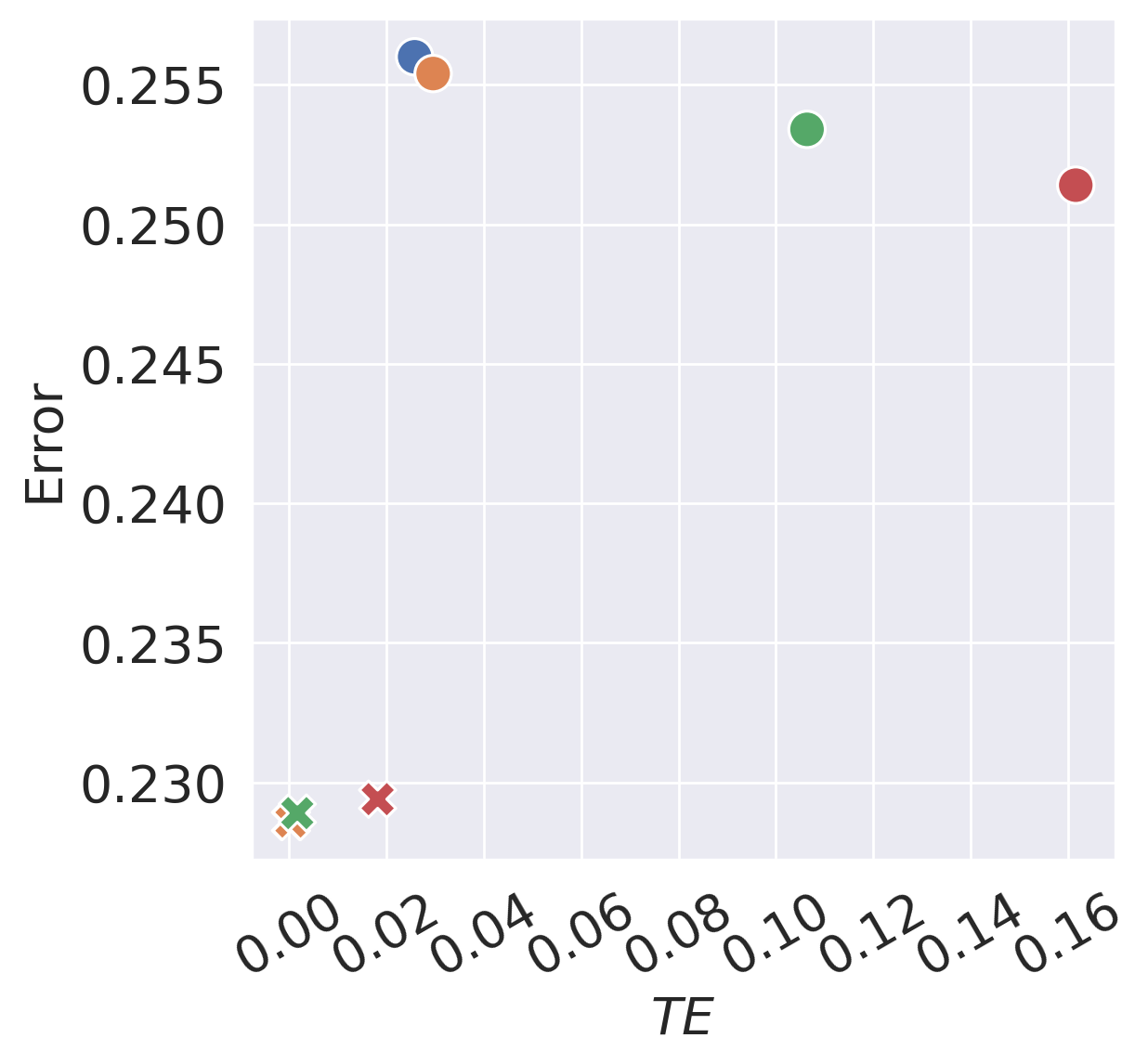
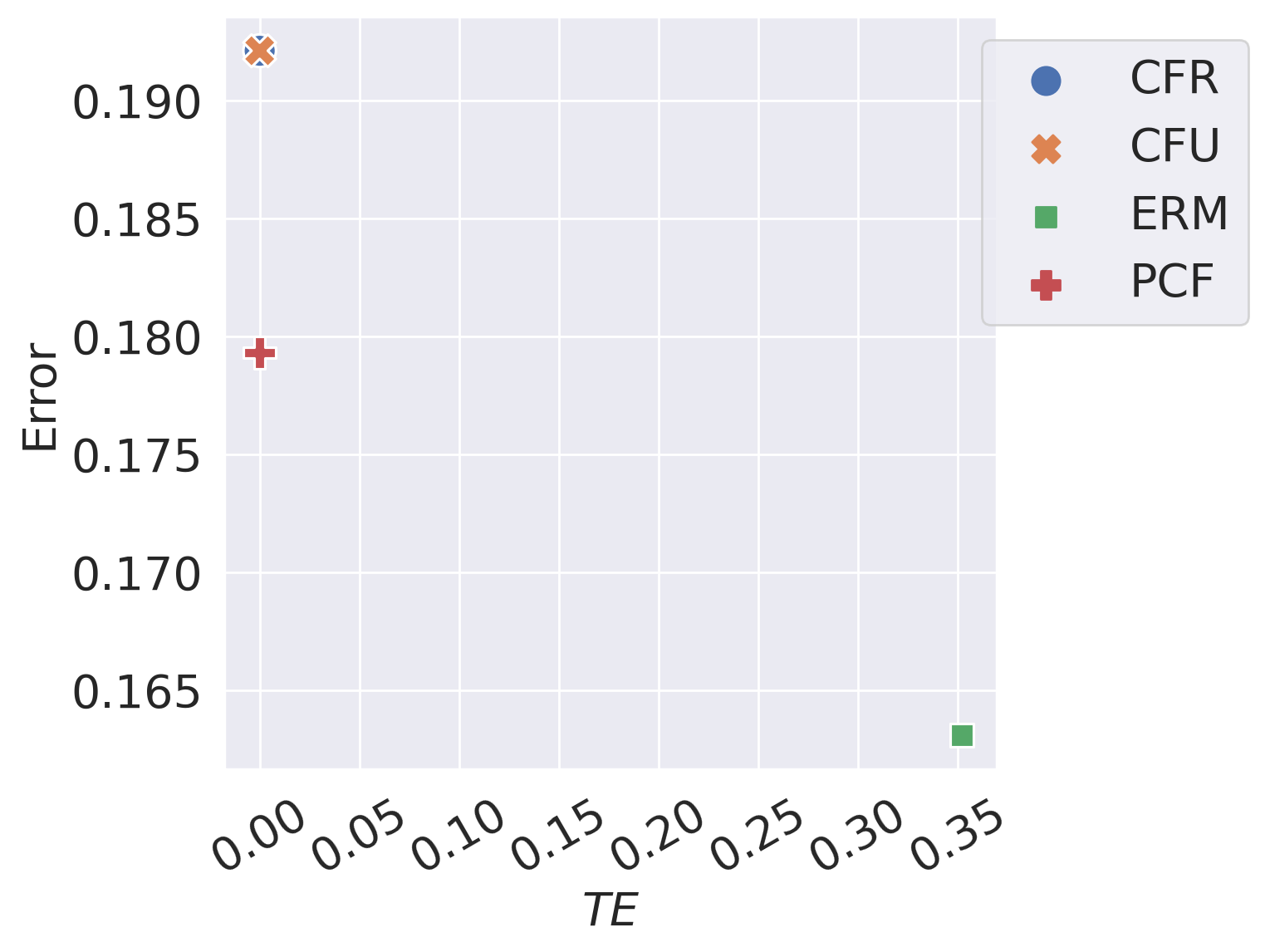
We consider two metrics in this paper: Error and Total Effect (TE). The former evaluates if each method can achieve its goal regardless of fair or not. This is important because we can achieve perfect Counterfactual Fairness by always outputing fixed prediction given whatever input, but that is not useful at all. The latter is a common metric to evaluate Counterfactual Fairness (Kim et al., 2021; Zuo et al., 2023). Given a test set , Error is defined as where is the ground truth target, is the prediction of , and depends on the task. TE is defined as where is the ground truth counterfactual corresponding to . Since we only consider binary sensitive attribute, we further define and to evaluate Counterfactual Fairness for different group respectively.
Methods
In general, we consider the following methods: (1) Empirical Risk Minimization (ERM): Directly train a classifier on all features without any fainress consideration. Specifically where represents the predictor. (2) Counterfactual Fairness with (CFU) (Kusner et al., 2017): To achieve Counterfactual Fairness, CFU proposes to use for prediction. Specifically, . (3) Counterfatual Fairness with fair representation (CFR) (Zuo et al., 2023): CFR proposes to use and a symmetric version of . Specifically, . (4) PCF333Essentially PCF with ERM (PCF-ERM). For brevity, we just call it PCF.: As introduced in Algorithm 1, PCF proposes to mix the output of factual and counterfactual prediction. Specifically, . (5) PCF with analytic solution (PCF-Ana): In our synthetic experiment, instead of training via ERM, we can directly acquire bayes optimal in closed-form. Detailed can be found in Section B.2. (6) PCF with CRM (PCF-CRM): As discussed in Section 3.3, it could be hard to get bayes optimal predictor, especially when there is counterfactual estimation error. Here due to the scale of our experiment, we choose to augment the dataset with estimated counterfactuals rather than finetuning. Specifically, is trained via ERM on the dataset .
5.1 Synthetic Dataset
In this section, we consider two regression synthetic datasets and two classification tasks where all of our assumptions in Assumption 3.1 are satisfied. The regression tasks are as below
The classification tasks take the same form except and for Linear-Cls and Cubic-Cls respectively. More details could be found in Section B.1. Results are averaged over 5 different runs where the structural model is kept the same but data is resampled. All results shown in the main paper use KNN based predictor. Results with other predictors can be found in Appendix C.
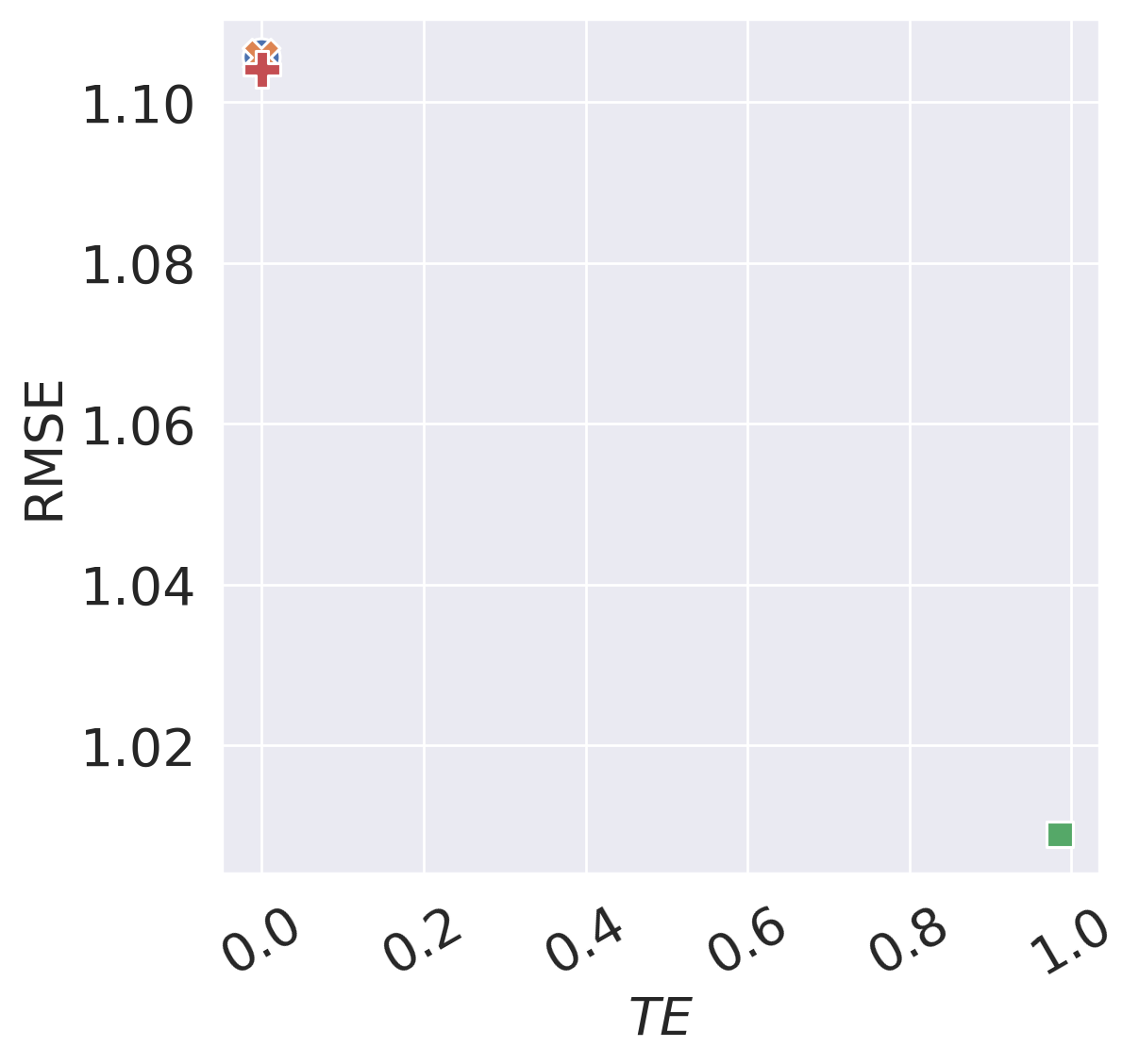
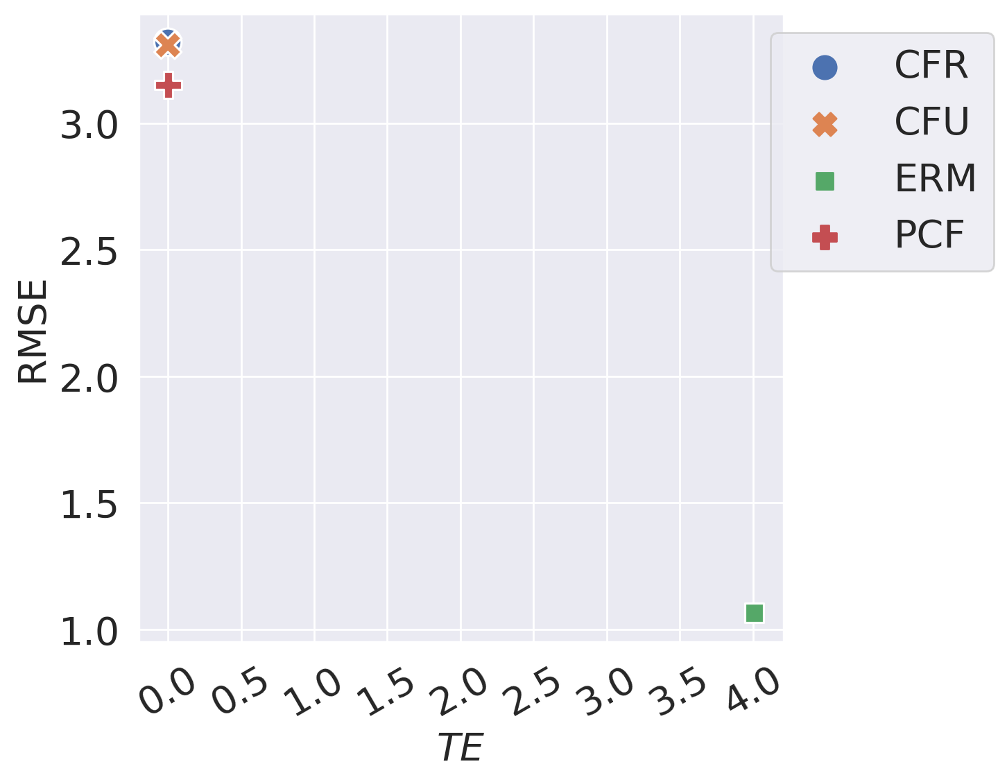
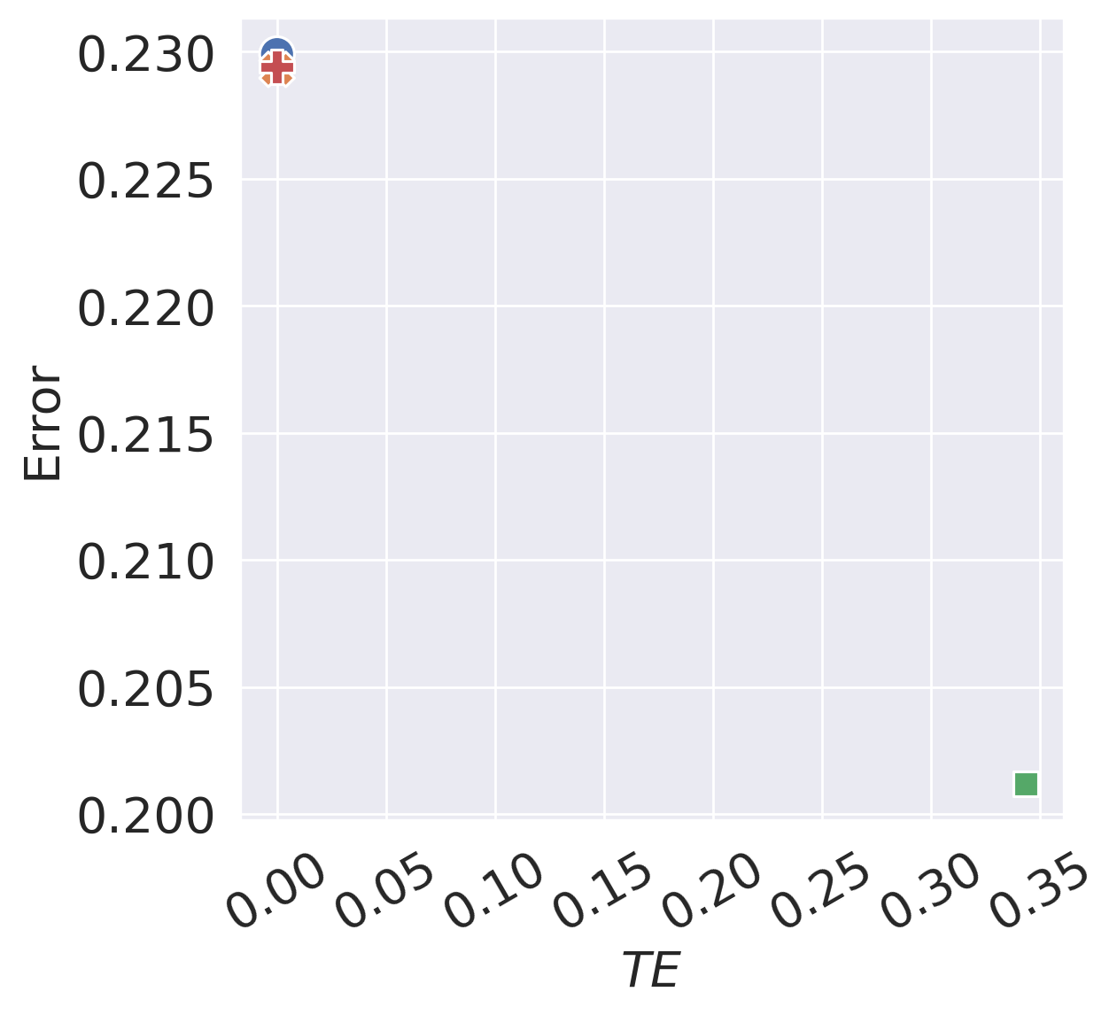
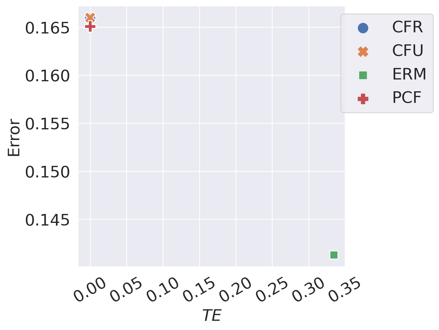
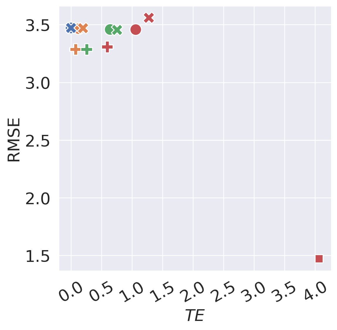
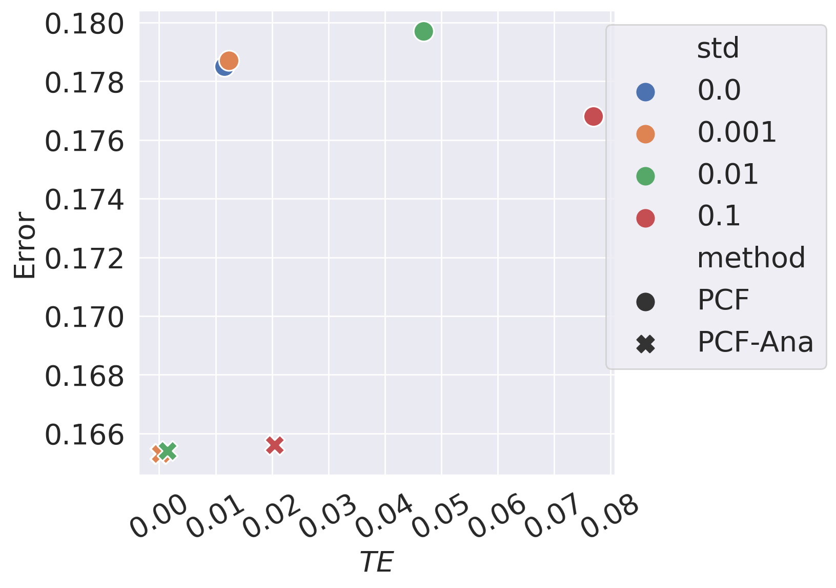
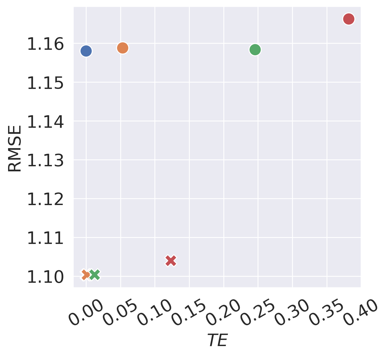
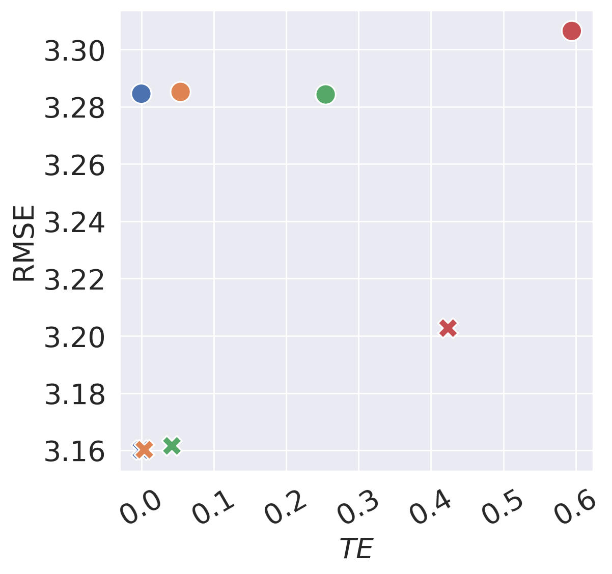
Optimality of PCF given true counterfactuals
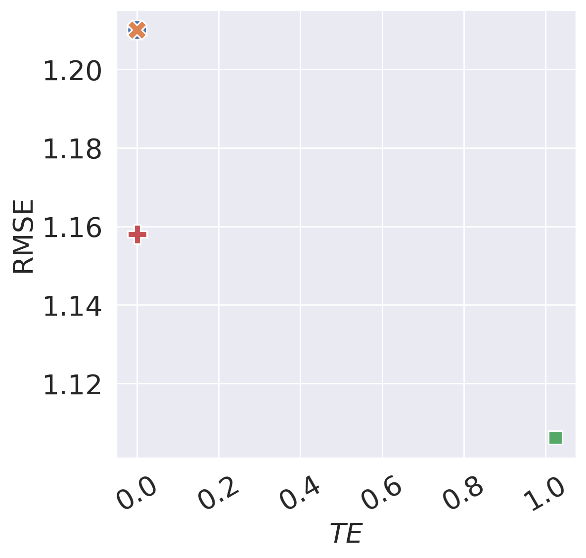
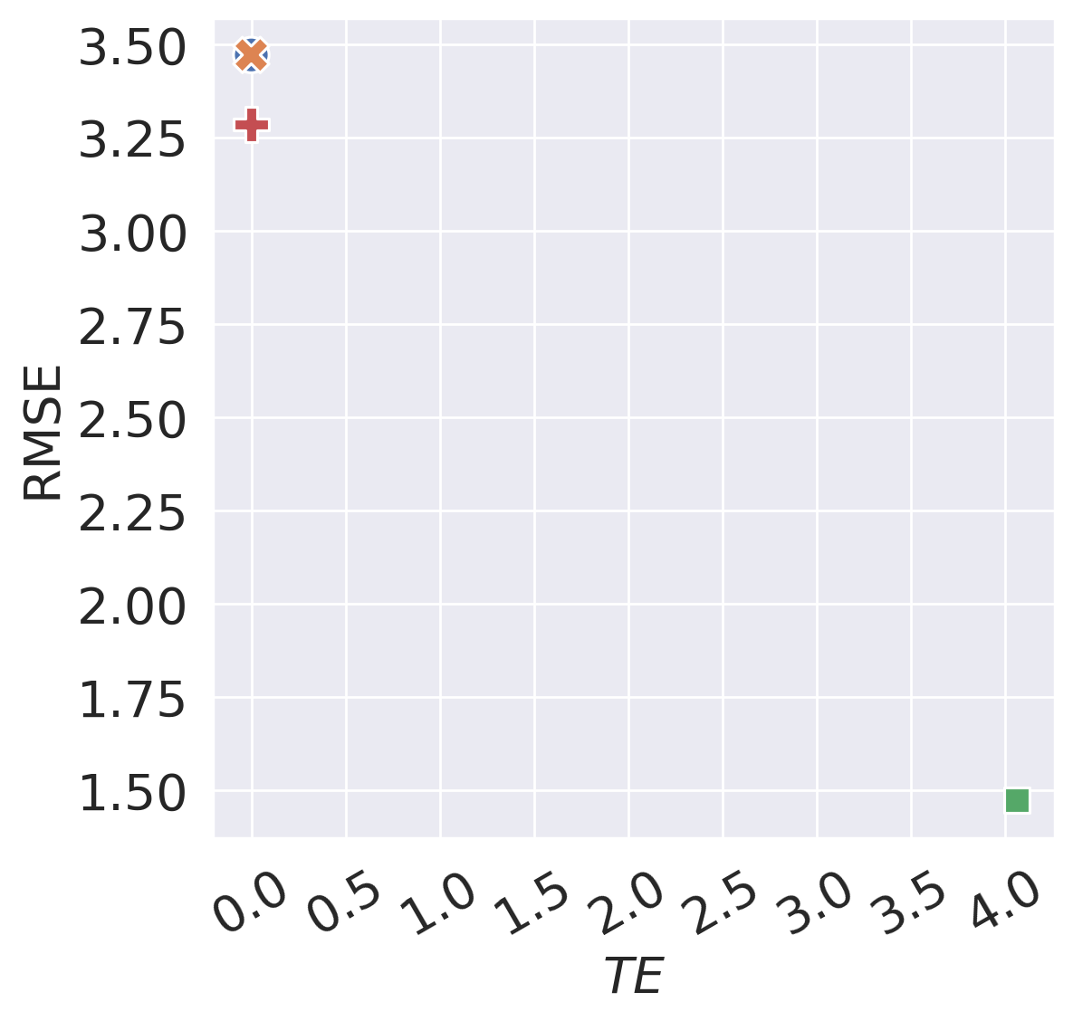
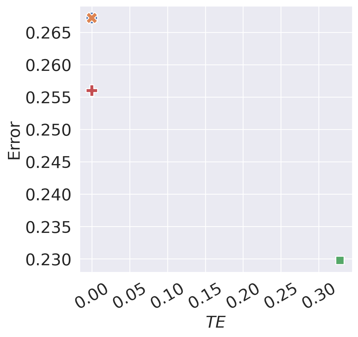
We first test different methods in situations where all methods have access to ground truth counterfactuals and as needed. In Figure 2, we observe that while CFE, CFR and PCF all achieve perfect CF, PCF has lowest predictor error. This validates Theorem 3.3 regarding the optimality of PCF under the constraint of CF. Furthermore, since here ERM can get solution close to optimal predictor (this indicates the plugin used by PCF is also close to being optimal), we can also observe the inherent fairness-utility trade-off discussed in Theorem 3.4.
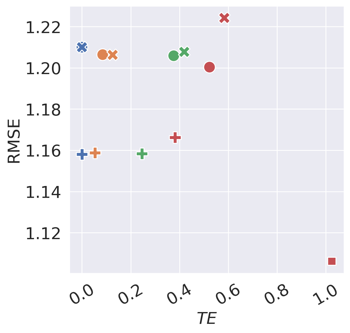

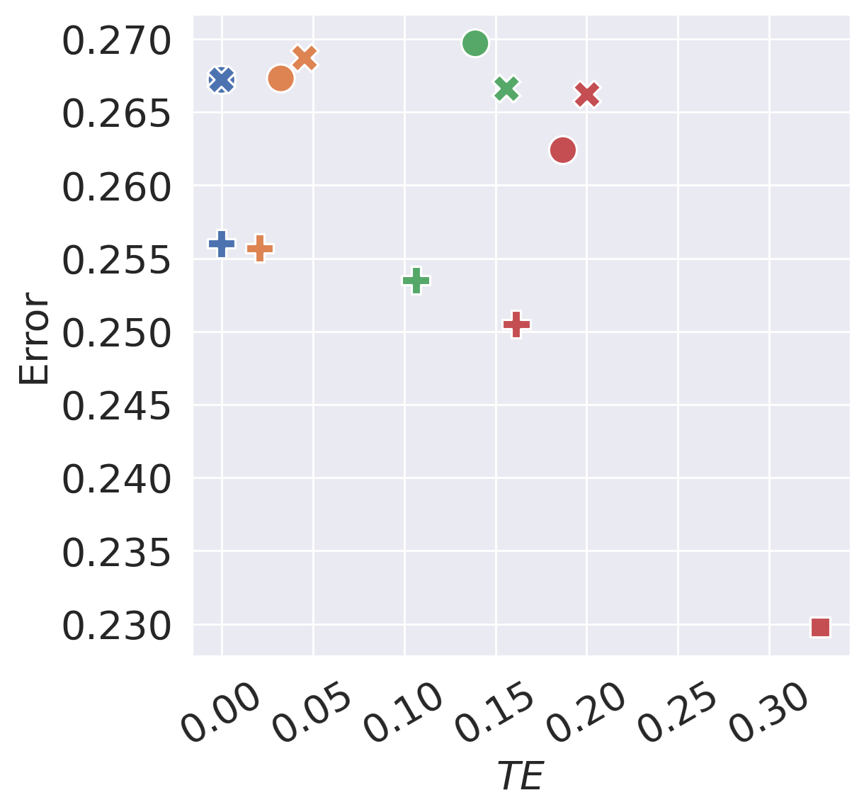
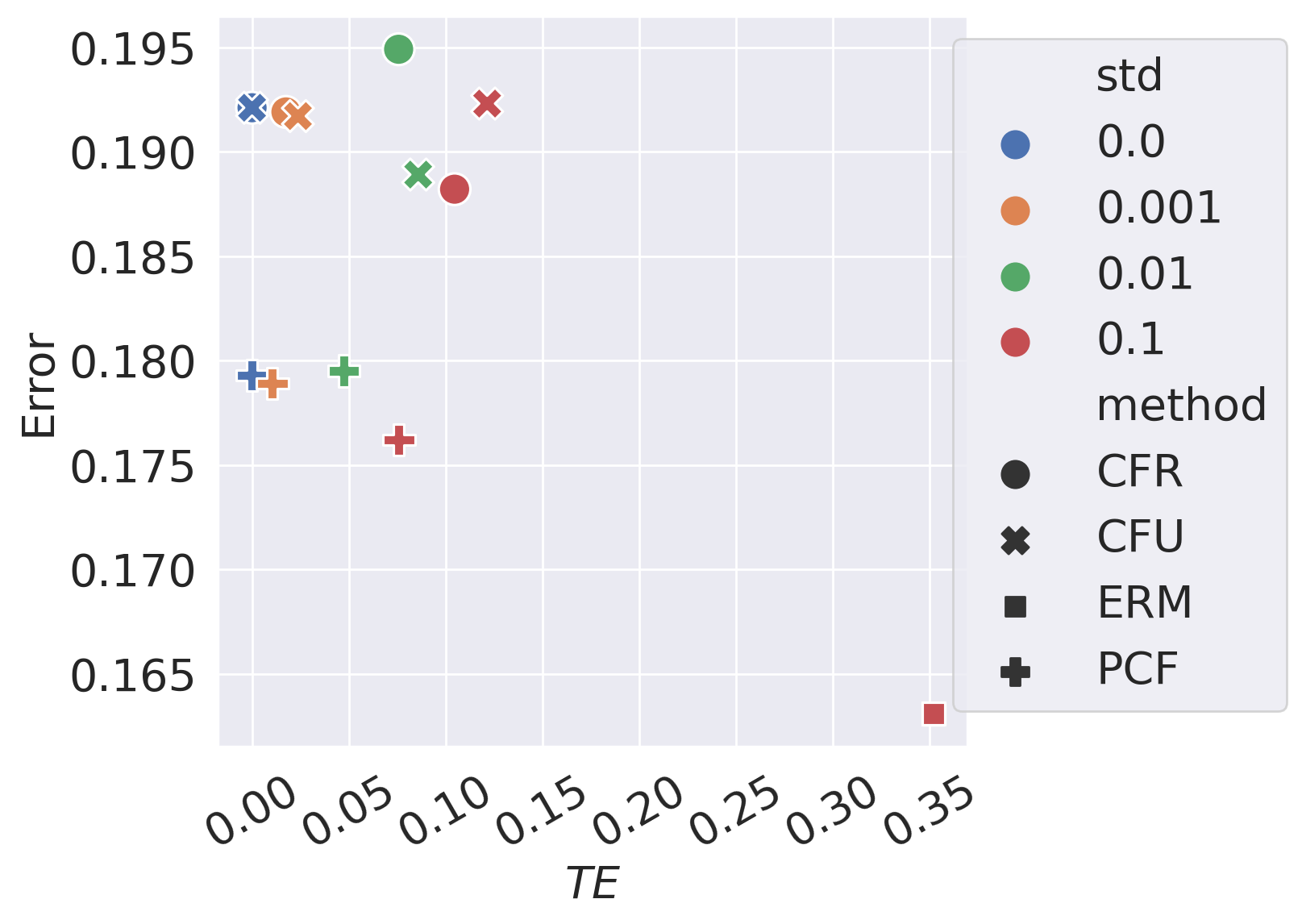
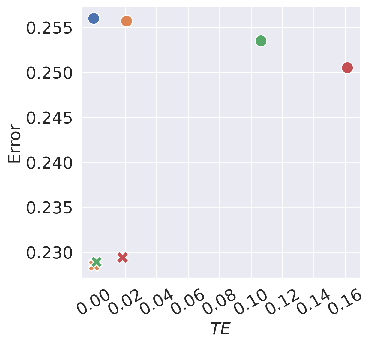
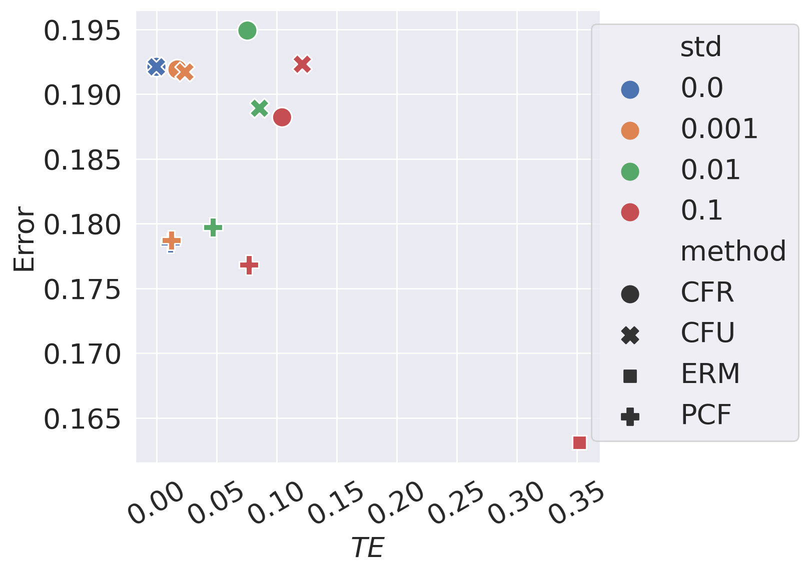
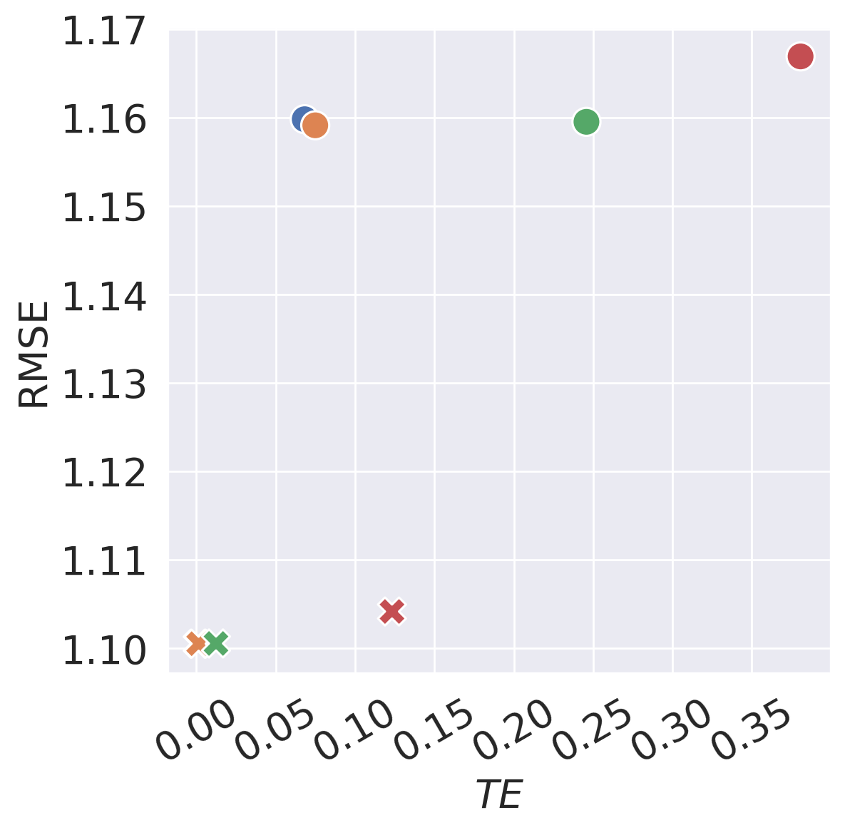
Performance under controllable error
Here we investigate a more practical scenario where both counterfactuals and need to be estimated. To investigate how error and TE changes with counterfactual estimation error in a more controllable way and investigate , we simulate the estimation error by adding gaussian noise. Specifically, and where . In Figure 3, we observe that while the fairness and ML performance (especially fairness) of CFE, CFR and PCF tends to get worse as error gets more significant, PCF remains best for all noise level.
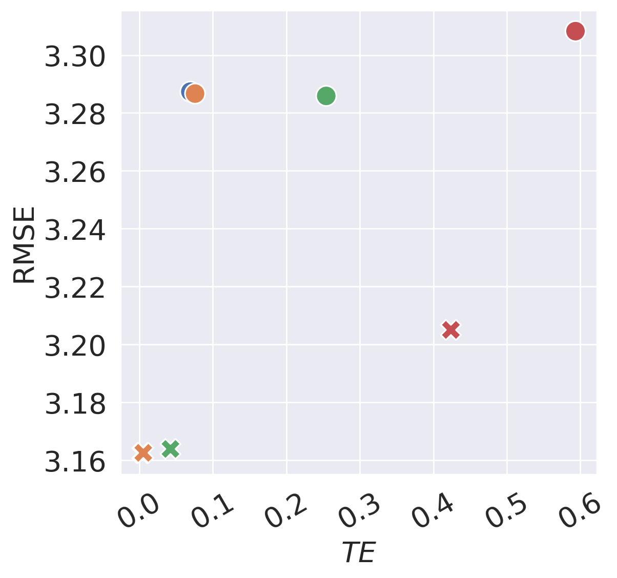
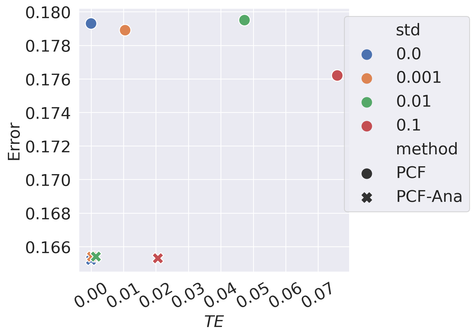
Investigating source of error
Here we further investigate what could be source of error in the previous scenario. As discussed in Section 3.3.2, in practice, two things in Theorem 3.3 break down: access to Bayes optimal classifier and ground truth counterfactuals. In Figure 4, we observe that PCF-Analytic tends to be more robust against counterfactual estimation error than PCF. We argue this is because used in PCF is not trained well on the estimated counterfactual distribution.
5.2 Semi-synthetic Dataset
We consider Law School Success dataset (Wightman, 1998) in this section. The main goal of this experiment is to validate the effectiveness of our methods in more practical scenarios where limited causal knowledge is available and the invertibility assumption is relaxed.
To compute TE, we need access to ground truth counterfactuals. Hence we train a generative model on real dataset to generate semi-synthetic dataset following the method in Zuo et al. (2023). Note that the counterfactuals are hidden from the algorithm and just used for evaluation. More details could be found in Section B.1. All experiments are repeated 5 times on the same semi-synthetic dataset.
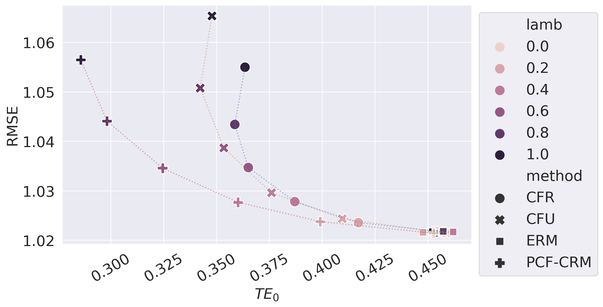
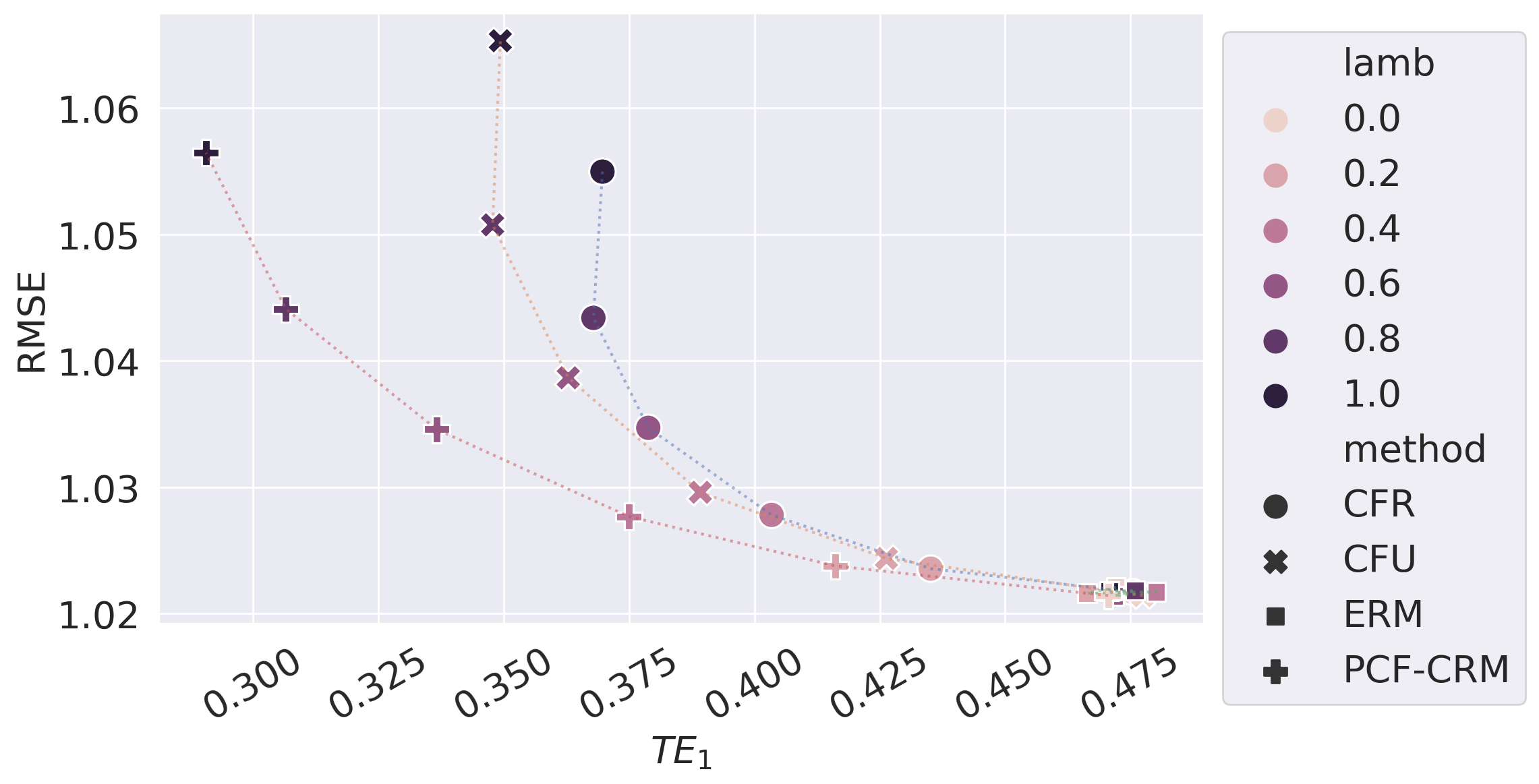
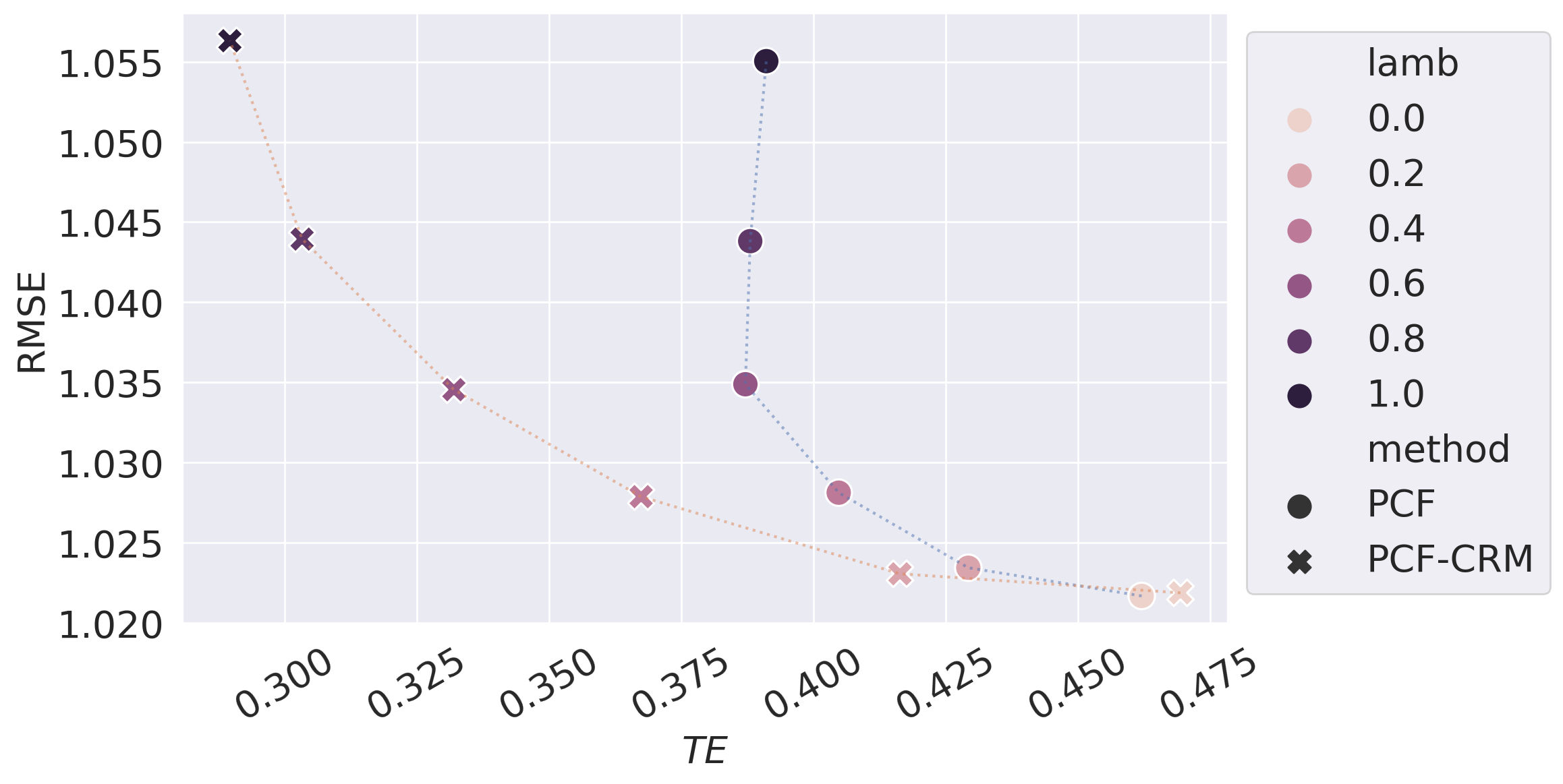
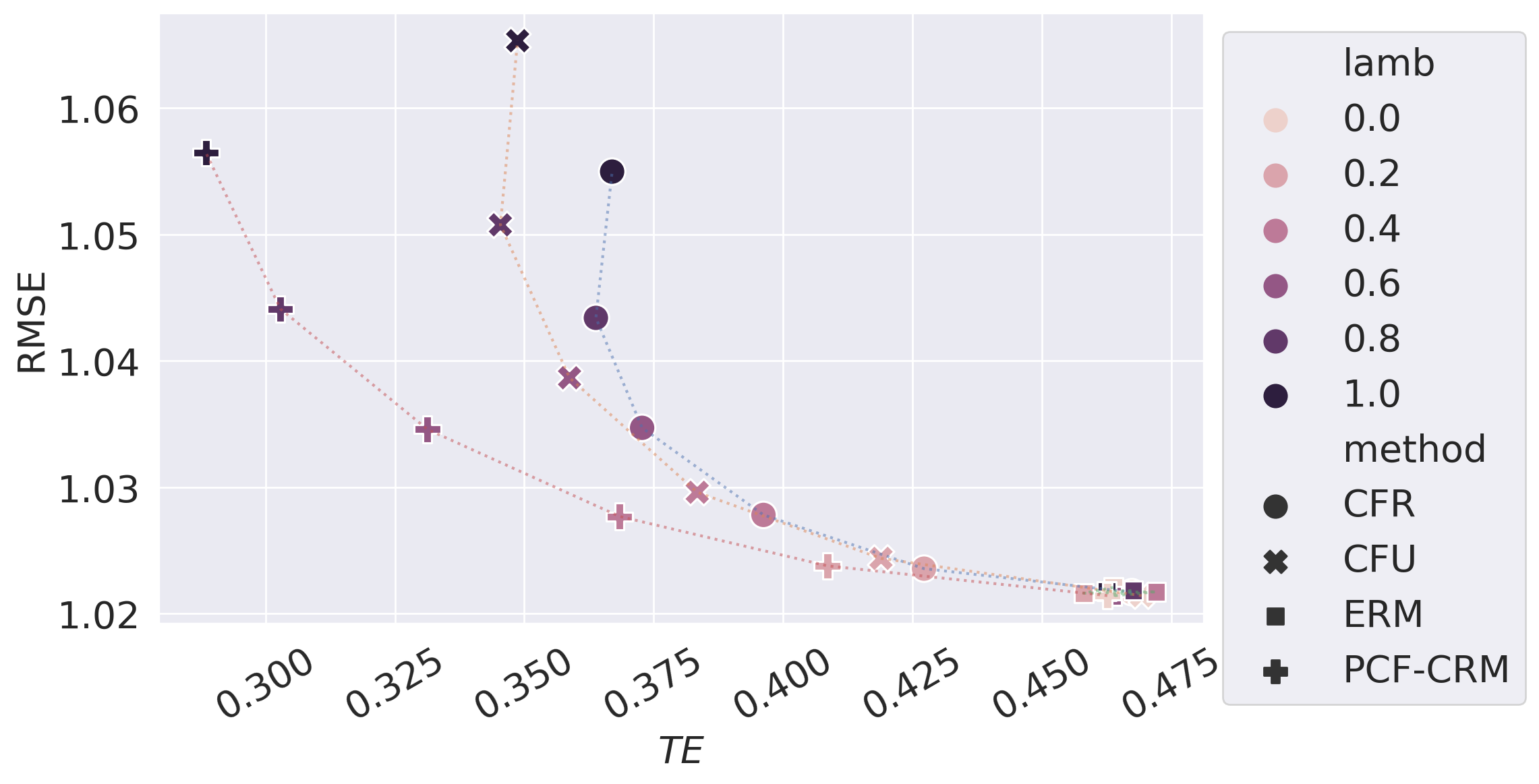
Results
In Figure 5, we observe that PCF-CRM achieves better CF and lower Error in comparison to CFU and CFR. This validates our improvement Section 3.3.2 indeed leads to more practical algorithm. Results on comparing PCF and PCF-CRM can be found in Appendix C, which further justifies this. While ERM could achieve lower error, it has worst fairness. This is inevitably determined by the inherent trade-off discussed in Theorem 3.4. Furthermore, inspired by the trade-off, we test the result of mixing all predictors with ERM. The curve shows that PCF-CRM remains optimal given fixed CF and best CF given fixed error. This demonstrates again that PCF-CRM is the best among all methods.
6 Conclusion and Discussion
Conclusion
In this work, we conducted a formal study on the trade-off between Counterfactual Fairness (CF) and predictive performance. We proved that combining factual and counterfactual predictions with a potentially unfair optimal predictor can achieve optimal CF. We also proved the excess risk between predictors with and without CF constraints, offering insights into the minimal predictiveness degradation needed for perfect CF. To address incomplete causal knowledge, we examined the impact of imperfect counterfactual estimations on CF and predictive performance. We proposed a plugin method using pre-trained models for optimal fair prediction and a practical approach to mitigate estimation inaccuracies.
Despite the theoretical merits of our method, there are two limitations that might raise concerns about its practical applicability: (1) access to ground truth counterfactuals and (2) access to Bayes optimal predictors. Here we discuss these limitations in more depth to bolster understanding of how our methods can be used in practice and how it can benefit from the broader community. Hopefully, this discussion will also inspire future research directions.
Access to ground truth counterfactuals
While how to better estimate counterfactuals is out of the scope of this work, it is indeed an unavoidable challenge faced by the community of Counterfactual Fairness. It not only limits the deployment of CF algorithms, but also leads to difficulty in validating proposed CF methods. There are some works in the field of causality that aims at estimating counterfactuals. For instance, Nasr-Esfahany et al. (2023) proves counterfactual identifiablity under certain causal graphs. However, in more general scenarios, we sometimes lack such knowledge, and identifying the causal graph itself can be challenging. These tasks have been well studied in the field of causal discovery (Chickering, 2002; Colombo et al., 2014) and causal representation learning (Schölkopf et al., 2021). Solutions to this problem typically rely on strong assumptions, such as the linearity of Structural Causal Models (SCMs) or additive noise (Shimizu et al., 2006; Hoyer et al., 2008; Peters et al., 2014). More recently, Zhou et al. (2024) proposes a method of estimating counterfactuals without need to identify the causal model or graph, which we believe have the potential to be a good plugin counnterfactual estimator in our algorithm.
Access to Bayes optimal predictors
Another crucial plugin estimator of our method is the optimal predictor. In classical ML settings, achieving a good estimator for the counterfactual distribution often requires retraining or fine-tuning. However, in this era, with the abundance of pre-trained models, such as foundation models (Bommasani et al., 2021), it could be much easier to get a predictor that is close to being optimal. Rather, given that these models are trained on noisy internet data and have extensive reach and impact, it is of great importance to find effective ways to debias them. We propose that our plugin algorithm could be a suitable solution due to its post-processing nature, which avoids incurring significant computational costs.
Acknowledgement
Z.Z., R.B., and D.I. acknowledge support from NSF (IIS-2212097), ARL (W911NF-2020221), and ONR (N00014-23-C-1016). M.K. acknowledges support from NSF CAREER 2239375, IIS 2348717, Amazon Research Award and Adobe Research. T.L. and J.G. acknowledge support from NSF-IIS2226108. Any opinions, findings, and conclusions or recommendations expressed in this material are those of the author(s) and do not necessarily reflect the views of any funding source.
References
- Anthis and Veitch (2024) Jacy Anthis and Victor Veitch. Causal context connects counterfactual fairness to robust prediction and group fairness. Advances in Neural Information Processing Systems, 36, 2024.
- Bolukbasi et al. (2016) Tolga Bolukbasi, Kai-Wei Chang, James Y Zou, Venkatesh Saligrama, and Adam T Kalai. Man is to computer programmer as woman is to homemaker? debiasing word embeddings. Advances in neural information processing systems, 29, 2016.
- Bommasani et al. (2021) Rishi Bommasani, Drew A Hudson, Ehsan Adeli, Russ Altman, Simran Arora, Sydney von Arx, Michael S Bernstein, Jeannette Bohg, Antoine Bosselut, Emma Brunskill, et al. On the opportunities and risks of foundation models. arXiv preprint arXiv:2108.07258, 2021.
- Brackey (2019) Adrienne Brackey. Analysis of Racial Bias in Northpointe’s COMPAS Algorithm. PhD thesis, Tulane University School of Science and Engineering, 2019.
- Brennan et al. (2009) Tim Brennan, William Dieterich, and Beate Ehret. Evaluating the predictive validity of the compas risk and needs assessment system. Criminal Justice and behavior, 36(1):21–40, 2009.
- Calders and Verwer (2010) Toon Calders and Sicco Verwer. Three naive bayes approaches for discrimination-free classification. Data mining and knowledge discovery, 21:277–292, 2010.
- Chen et al. (2018) Irene Chen, Fredrik D Johansson, and David Sontag. Why is my classifier discriminatory? Advances in neural information processing systems, 31, 2018.
- Chiappa (2019) Silvia Chiappa. Path-specific counterfactual fairness. In Proceedings of the AAAI conference on artificial intelligence, volume 33, pages 7801–7808, 2019.
- Chickering (2002) David Maxwell Chickering. Optimal structure identification with greedy search. Journal of machine learning research, 3(Nov):507–554, 2002.
- Chzhen et al. (2020) Evgenii Chzhen, Christophe Denis, Mohamed Hebiri, Luca Oneto, and Massimiliano Pontil. Fair regression with wasserstein barycenters. Advances in Neural Information Processing Systems, 33:7321–7331, 2020.
- Colombo et al. (2014) Diego Colombo, Marloes H Maathuis, et al. Order-independent constraint-based causal structure learning. J. Mach. Learn. Res., 15(1):3741–3782, 2014.
- Corbett-Davies et al. (2023) Sam Corbett-Davies, Johann D Gaebler, Hamed Nilforoshan, Ravi Shroff, and Sharad Goel. The measure and mismeasure of fairness. The Journal of Machine Learning Research, 24(1):14730–14846, 2023.
- Daneshjou et al. (2021) Roxana Daneshjou, Kailas Vodrahalli, Weixin Liang, Roberto A Novoa, Melissa Jenkins, Veronica Rotemberg, Justin Ko, Susan M Swetter, Elizabeth E Bailey, Olivier Gevaert, et al. Disparities in dermatology ai: assessments using diverse clinical images. arXiv preprint arXiv:2111.08006, 2021.
- Donini et al. (2018) Michele Donini, Luca Oneto, Shai Ben-David, John S Shawe-Taylor, and Massimiliano Pontil. Empirical risk minimization under fairness constraints. Advances in neural information processing systems, 31, 2018.
- Dwork et al. (2012) Cynthia Dwork, Moritz Hardt, Toniann Pitassi, Omer Reingold, and Richard Zemel. Fairness through awareness. In Proceedings of the 3rd innovations in theoretical computer science conference, pages 214–226, 2012.
- Farahani et al. (2021) Abolfazl Farahani, Sahar Voghoei, Khaled Rasheed, and Hamid R Arabnia. A brief review of domain adaptation. Advances in data science and information engineering: proceedings from ICDATA 2020 and IKE 2020, pages 877–894, 2021.
- Galhotra et al. (2022) Sainyam Galhotra, Karthikeyan Shanmugam, Prasanna Sattigeri, and Kush R Varshney. Causal feature selection for algorithmic fairness. In Proceedings of the 2022 International Conference on Management of Data, pages 276–285, 2022.
- Garg et al. (2019) Sahaj Garg, Vincent Perot, Nicole Limtiaco, Ankur Taly, Ed H. Chi, and Alex Beutel. Counterfactual fairness in text classification through robustness. In Proceedings of the 2019 AAAI/ACM Conference on AI, Ethics, and Society, AIES 2019, Honolulu, HI, USA, January 27-28, 2019, pages 219–226, 2019.
- Grari et al. (2023) Vincent Grari, Sylvain Lamprier, and Marcin Detyniecki. Adversarial learning for counterfactual fairness. Mach. Learn., 112(3):741–763, 2023. doi: 10.1007/S10994-022-06206-8. URL https://doi.org/10.1007/s10994-022-06206-8.
- Grgic-Hlaca et al. (2016) Nina Grgic-Hlaca, Muhammad Bilal Zafar, Krishna P Gummadi, and Adrian Weller. The case for process fairness in learning: Feature selection for fair decision making. In NIPS symposium on machine learning and the law, volume 1, page 11. Barcelona, Spain, 2016.
- Hardt et al. (2016) Moritz Hardt, Eric Price, and Nati Srebro. Equality of opportunity in supervised learning. Advances in neural information processing systems, 29, 2016.
- Hoffman et al. (2018) Mitchell Hoffman, Lisa B Kahn, and Danielle Li. Discretion in hiring. The Quarterly Journal of Economics, 133(2):765–800, 2018.
- Hoyer et al. (2008) Patrik Hoyer, Dominik Janzing, Joris M Mooij, Jonas Peters, and Bernhard Schölkopf. Nonlinear causal discovery with additive noise models. Advances in neural information processing systems, 21, 2008.
- Jang et al. (2022) Taeuk Jang, Pengyi Shi, and Xiaoqian Wang. Group-aware threshold adaptation for fair classification. In Proceedings of the AAAI Conference on Artificial Intelligence, volume 36, pages 6988–6995, 2022.
- Kamiran and Calders (2012) Faisal Kamiran and Toon Calders. Data preprocessing techniques for classification without discrimination. Knowledge and information systems, 33(1):1–33, 2012.
- Khademi et al. (2019) Aria Khademi, Sanghack Lee, David Foley, and Vasant Honavar. Fairness in algorithmic decision making: An excursion through the lens of causality. In The World Wide Web Conference, pages 2907–2914, 2019.
- Khandani et al. (2010) Amir E Khandani, Adlar J Kim, and Andrew W Lo. Consumer credit-risk models via machine-learning algorithms. Journal of Banking & Finance, 34(11):2767–2787, 2010.
- Kim et al. (2021) Hyemi Kim, Seungjae Shin, JoonHo Jang, Kyungwoo Song, Weonyoung Joo, Wanmo Kang, and Il-Chul Moon. Counterfactual fairness with disentangled causal effect variational autoencoder. In Proceedings of the AAAI Conference on Artificial Intelligence, volume 35, pages 8128–8136, 2021.
- Kusner et al. (2017) Matt J Kusner, Joshua Loftus, Chris Russell, and Ricardo Silva. Counterfactual fairness. Advances in neural information processing systems, 30, 2017.
- Liu et al. (2023) Tianci Liu, Haoyu Wang, Yaqing Wang, Xiaoqian Wang, Lu Su, and Jing Gao. Simfair: A unified framework for fairness-aware multi-label classification. Proceedings of the AAAI Conference on Artificial Intelligence, 37(12):14338–14346, 2023.
- Lohaus et al. (2020) Michael Lohaus, Michael Perrot, and Ulrike Von Luxburg. Too relaxed to be fair. In International Conference on Machine Learning, pages 6360–6369, 2020.
- Makhlouf et al. (2022) Karima Makhlouf, Sami Zhioua, and Catuscia Palamidessi. Survey on causal-based machine learning fairness notions, 2022.
- Menon and Williamson (2018) Aditya Krishna Menon and Robert C Williamson. The cost of fairness in binary classification. In Conference on Fairness, accountability and transparency, pages 107–118, 2018.
- Mohler et al. (2018) George Mohler, Rajeev Raje, Jeremy Carter, Matthew Valasik, and Jeffrey Brantingham. A penalized likelihood method for balancing accuracy and fairness in predictive policing. In 2018 IEEE international conference on systems, man, and cybernetics (SMC), pages 2454–2459. IEEE, 2018.
- Nasr-Esfahany et al. (2023) Arash Nasr-Esfahany, Mohammad Alizadeh, and Devavrat Shah. Counterfactual identifiability of bijective causal models. arXiv preprint arXiv:2302.02228, 2023.
- Nilforoshan et al. (2022) Hamed Nilforoshan, Johann D Gaebler, Ravi Shroff, and Sharad Goel. Causal conceptions of fairness and their consequences. In International Conference on Machine Learning, pages 16848–16887. PMLR, 2022.
- Pearl (2009) Judea Pearl. Causality. Cambridge university press, 2009.
- Pedreshi et al. (2008) Dino Pedreshi, Salvatore Ruggieri, and Franco Turini. Discrimination-aware data mining. In Proceedings of the 14th ACM SIGKDD international conference on Knowledge discovery and data mining, pages 560–568, 2008.
- Pessach and Shmueli (2023) Dana Pessach and Erez Shmueli. Algorithmic Fairness, pages 867–886. 2023.
- Peters et al. (2014) Jonas Peters, Joris M Mooij, Dominik Janzing, and Bernhard Schölkopf. Causal discovery with continuous additive noise models. 2014.
- Petersen et al. (2021) Felix Petersen, Debarghya Mukherjee, Yuekai Sun, and Mikhail Yurochkin. Post-processing for individual fairness. Advances in Neural Information Processing Systems, 34:25944–25955, 2021.
- Plecko and Bareinboim (2022) Drago Plecko and Elias Bareinboim. Causal fairness analysis. arXiv preprint arXiv:2207.11385, 2022.
- Rosenblatt and Witter (2023a) Lucas Rosenblatt and R. Teal Witter. Counterfactual fairness is basically demographic parity, 2023a.
- Rosenblatt and Witter (2023b) Lucas Rosenblatt and R. Teal Witter. Counterfactual fairness is basically demographic parity. In Brian Williams, Yiling Chen, and Jennifer Neville, editors, Thirty-Seventh AAAI Conference on Artificial Intelligence, AAAI 2023, pages 14461–14469. AAAI Press, 2023b. doi: 10.1609/AAAI.V37I12.26691. URL https://doi.org/10.1609/aaai.v37i12.26691.
- Schölkopf et al. (2021) Bernhard Schölkopf, Francesco Locatello, Stefan Bauer, Nan Rosemary Ke, Nal Kalchbrenner, Anirudh Goyal, and Yoshua Bengio. Toward causal representation learning. Proceedings of the IEEE, 109(5):612–634, 2021.
- Scutari et al. (2021) Marco Scutari, Francesca Panero, and Manuel Proissl. Achieving fairness with a simple ridge penalty, 2021.
- Shimizu et al. (2006) Shohei Shimizu, Patrik O Hoyer, Aapo Hyvärinen, Antti Kerminen, and Michael Jordan. A linear non-gaussian acyclic model for causal discovery. Journal of Machine Learning Research, 7(10), 2006.
- Stefano et al. (2020) Pietro G. Di Stefano, James M. Hickey, and Vlasios Vasileiou. Counterfactual fairness: removing direct effects through regularization. CoRR, abs/2002.10774, 2020.
- Wightman (1998) Linda F Wightman. Lsac national longitudinal bar passage study. lsac research report series. 1998.
- Wu et al. (2019) Yongkai Wu, Lu Zhang, and Xintao Wu. Counterfactual fairness: Unidentification, bound and algorithm. In Proceedings of the Twenty-Eighth International Joint Conference on Artificial Intelligence, IJCAI-19, pages 1438–1444, 2019.
- Xian et al. (2023) Ruicheng Xian, Lang Yin, and Han Zhao. Fair and optimal classification via post-processing. In International Conference on Machine Learning, pages 37977–38012. PMLR, 2023.
- Zafar et al. (2017) Muhammad Bilal Zafar, Isabel Valera, Manuel Gomez Rodriguez, and Krishna P Gummadi. Fairness beyond disparate treatment & disparate impact: Learning classification without disparate mistreatment. In Proceedings of the 26th international conference on world wide web, pages 1171–1180, 2017.
- Zhao and Gordon (2022) Han Zhao and Geoffrey J. Gordon. Inherent tradeoffs in learning fair representations, 2022.
- Zhou et al. (2022) Kaiyang Zhou, Ziwei Liu, Yu Qiao, Tao Xiang, and Chen Change Loy. Domain generalization: A survey. IEEE Transactions on Pattern Analysis and Machine Intelligence, 45(4):4396–4415, 2022.
- Zhou et al. (2024) Zeyu Zhou, Ruqi Bai, Sean Kulinski, Murat Kocaoglu, and David I Inouye. Towards characterizing domain counterfactuals for invertible latent causal models. In The Twelfth International Conference on Learning Representations, 2024. URL https://openreview.net/forum?id=v1VvCWJAL8.
- Zuo et al. (2023) Zhiqun Zuo, Mohammad Mahdi Khalili, and Xueru Zhang. Counterfactually fair representation. Advances in neural information processing systems, 2023.
Appendix A Proofs
A.1 Proof of Lemma 3.2
Proof of Lemma 3.2.
| (1) |
where the first equality is by definition and the second equality is because absolute value is always non-negative for any . Thus, the predictions must be almost surely equal for all . Similarly, if they are all equal on the non-zero metric set, then the expectation must be 0. ∎
A.2 Proof of Theorem 3.3
Before proving the main theorem, we first provide one well-known lemma that reminds the reader of the well-known result of the optimal predictor, which is denoted by in the theorem statement.
Lemma A.1 (Optimal Predictor is Conditional Mean).
The conditional mean is the optimal predictor without fairness constraints for classification with cross-entropy loss and for regression with MSE loss.
Proof.
First, let’s establish that the optimal predictor without constraints is in fact . For squared loss, we have that derivative:
Taking the derivative of the inside expectation w.r.t. and setting to 0 yields .
Now let’s look at cross-entropy loss for classification:
Again, if you take the derivative w.r.t. and set to 0, we see that . ∎
Now we seek to prove Theorem 3.3.
Proof.
First, we decompose the factual error across the sensitive attribute given the exogenous noise .
Consider inside the expectation we have
where w.l.o.g., is viewed as the factual and is viewed as the counterfactual. Because of invertibility, these two terms are unique for every or correspondingly combination and thus the problem decomposes across . Thus, the factual loss can be viewed as a combination of the factual loss from one specific plus the counterfactual loss for for each point .
We have the following subproblems indexed by : The factual loss can be viewed as a combination of the factual loss from one specific plus the counterfactual loss for for each point . Notice that the constraint is from Lemma 3.2. We can directly push the constraint into the optimization problem by optimizing over :
| (2) |
Taking as squared loss: we have
Similarly, if we take as (binary) cross-entropy loss: we have
It is simple to see that both loss functions are convex, thus could obtain a unique solution by taking the derivative. Thus, for each induced by , we could get the optimal :
where is the optimal predictor from the lemma above. This result holds for every and thus gives the final result. ∎
A.3 Proof of Theorem 3.4
Proof.
Let and be the Bayes optimal predictor under no constraint and CF constraint respectively. We have shown that and .
Noting that is Bayes optimal, its risk satisfies where denotes the risk of . By definition, the excess risk of is
For regression task and real-valued , we take as squared loss and have
Let’s define
where holds from the invertibility between and given , and holds from the fact that and are independent. For simplicity, we denote . Notably, measures the expected change of due to the change of over all possible , and is in fact a measure of their dependency. Furthermore, we have
Next, for classification task and binary using cross-entropy loss, then
where holds from noting that and , and again holds from the invertibility between and given . ∎
A.4 Proof of Proposition 3.5
Proof.
where the middle qualities are by the properties of the invertible and ground truth CGM. Because the factual output for the algorithm is the same as the counterfactual output, then the TE must be 0 by Lemma 3.2. ∎
A.5 Proof of Theorem 3.6
Proof.
We first bound TE.
Let , we have
Here holds by the convexity of absolute value, is from the L-lipschitz property of , and is by the bound of counterfactual estimation error.
Now we prove the bound for the error. Taking as squared loss, we have
Taking the inner expectation and omit subscript for brevity, we have
where denotes the remaining term that only depends on . Here holds from the fact that the counterfactual estimation error is bounded by and the assumption that is -lipschitz.
Next, take the outer expectation,
Note that taking expectation of with respect to the joint distribution of is in fact the optimal risk . Reorganization gives us
∎
Appendix B Experiment Details
We included the codes to reproduce our results. All GPU related experiments are run on RTX A5000.
B.1 Dataset
Synthetic Dataset
In this section, we consider the two regression synthetic datasets and two classification tasks where all of our assumptions in Assumption 3.1 are satisfied.
where in our experiments the parameters are chosen as .
We also consider the following two classification tasks
where in our experiments the parameters are chosen as .
Semi-synthetic Dataset
We consider Law School Success [Wightman, 1998]. The sensitive attribute is gender and the target is first-year grade. Other features contain race, LSAT and GPA. However, since we need to evaluate TE of each method which requires access to ground truth, we use the simulated version of those datasets. Following a similar setup in [Zuo et al., 2023], we train a generative model to get semi-synthetic datasets. Specifically, we train a VAE with the following structure , , . The training objective includes a normal VAE objective to reconstruct via and , and a supervised objective to generate via . After training, we first sample a prior and (where is acquired based on empirical frequency in real data), then we get the semi-synthetic using and . We want to emphasize that counterfactuals, regardless of train or test set, are hidden from downstream models and used for evaluation only. This way, we get access to the ground truth and can generate ground truth counterfactuals without any error. In our investigation, exogenous noise, factual data and counterfactual data are all actually the simulated version of original datasets. However they do follow a fixed data generating mechanism that is close to the real data.
B.2 Analytic Solution on Synthetic Datasets
We know the analytic solution of Bayes optimal predictor in our synthetic data experiments. More specifically, for Linear-Reg, we have
For Cubic-Reg, we have
For Linear-Cls, we have
For Cubic-Cls, we have
B.3 Prediction Models
In our synthetic experiments, we mainly use KNN based predictors. We use the default parameters in scikit-learn. All MLP methods uses a structure with hidden layer and Tanh activation.
In semi-synthetic experiments, we use MLP methods uses a structure with hidden layer and Tanh activation as this is closer to the ground truth SCM.
Appendix C Additional Results
C.1 Additional results on synthetic datasets
In Figure 6, we test how how all algorithms perform when using ground truth counterfactuals and on additional type of predictors. We observe that PCF achieves lower error than CFU and CFR, which is similar to what we observe in Figure 2. This further validates our theory regarding optimality of PCF.
In Figure 7, following the investigation in Figure 3, we test with adding gaussian noise with different mean. We observe that when it is a fixed bias, CFU and CFR achieves better fairness than PCF. Though PCF still achieves best predictive performance. Furthermore, as we increase variance of the noise, PCF outperform these two methods in terms of both fairness and ML performance. In Figure 8, similar to Figure 4, we observe PCF-Analytic significantly improves over PCF. Notably, it is not affected by bias as PCF.
C.2 Additional results on semi-synthetic datasets
In Figure 9, we included the expanded version of Figure 5 with and . We observe that they show very similar trend. In Figure 10, we directly compare PCF (with ERM) and PCF-CRM. The results validate the necessity of CRM as a plugin estimator in the case of limited causal knowledge.