$k$-span weakly leveled planarity

Weakly Leveled Planarity with Bounded Span

Abstract

This paper studies planar drawings of graphs in which each vertex is represented as a point along a sequence of horizontal lines, called levels, and each edge is either a horizontal segment or a strictly $y$-monotone curve. A graph is $s$-span weakly leveled planar if it admits such a drawing where the edges have span at most $s$; the span of an edge is the number of levels it touches minus one. We investigate the problem of computing $s$-span weakly leveled planar drawings from both the computational and the combinatorial perspectives. We prove the problem to be para-NP-hard with respect to its natural parameter $s$ and investigate its complexity with respect to widely used structural parameters. We show the existence of a polynomial-size kernel with respect to vertex cover number and prove that the problem is FPT when parameterized by treedepth. We also present upper and lower bounds on the span for various graph classes. Notably, we show that cycle trees, a family of $2$-outerplanar graphs generalizing Halin graphs, are $\Theta(\log n)$-span weakly leveled planar and $4$-span weakly leveled planar when $3$-connected. As a byproduct of these combinatorial results, we obtain improved bounds on the edge-length ratio of the graph families under consideration.

1 Introduction

Computing crossing-free drawings of planar graphs is at the heart of Graph Drawing. Indeed, since the seminal papers by Fáry [Far48] and by Tutte [tutte1963draw] were published, a rich body of literature has been devoted to the study of crossing-free drawings of planar graphs that satisfy a variety of optimization criteria, including the area [DBLP:journals/algorithmica/Kant96, DBLP:journals/combinatorica/FraysseixPP90], the angular resolution [DBLP:journals/siamcomp/FormannHHKLSWW93, DBLP:journals/siamdm/MalitzP94], the face convexity [DBLP:journals/ijcga/ChrobakK97, DBLP:conf/gd/BonichonFM04, DBLP:journals/algorithmica/BonichonFM07], the total edge length [DBLP:journals/siamcomp/Tamassia87], and the edge-length ratio [DBLP:conf/gd/BorrazzoF19, DBLP:journals/jocg/BorrazzoF20, DBLP:journals/ijcga/BlazjFL21]; see also [BattistaETT99, Tamassia:13].

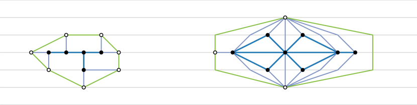
Figure 1: A $1$-span weakly leveled planar drawing of the Frucht graph (left) and a $4$-span weakly leveled planar drawing of the Goldner-Harary graph (right).

In this paper, we focus on crossing-free drawings where the edges are represented as simple Jordan arcs and have the additional constraint of being $y$-monotone, that is, traversing each edge from one end-vertex to the other one, the $y$-coordinates never increase or never decrease. This leads to a generalization of the well-known layered drawing style [DBLP:journals/algorithmica/DujmovicFKLMNRRWW08, DBLP:conf/gd/BrucknerKM19, DBLP:journals/algorithmica/BrucknerKM22], where vertices are assigned to horizontal lines, called levels, and edges only connect vertices on different levels. We also allow edges between vertices on the same level and seek for drawings of bounded span, i.e., in which the edges span few levels. In their seminal work [DBLP:journals/siamcomp/HeathR92], Heath and Rosenberg study leveled planar drawings, i.e., in which edges only connect vertices on consecutive levels and no two edges cross. We also mention the algorithmic framework by Sugiyama et al. [DBLP:journals/tsmc/SugiyamaTT81], which yields layered drawings for the so-called hierarchical graphs. In this framework, edges that span more than one level are transformed into paths by inserting a dummy vertex for each level they cross. Hence minimizing the edge span (or equivalently, the number of dummy vertices along the edges) is a relevant optimization criterion.

Inspired by these works, we study $s$-span weakly leveled planar drawings, which are crossing-free $y$-monotone drawings in which each edge touches at most $s+1$ levels; see Fig. 1. Note that 1-span weakly leveled planar drawings have been studied in different contexts; for example, Bannister et al. [DBLP:conf/dagstuhl/BastertM99] prove that graphs that admit such drawings have layered pathwidth at most two. Felsner et al. [DBLP:conf/gd/FelsnerLW01, DBLP:journals/jgaa/FelsnerLW03] show that every outerplanar graph has a 1-span weakly leveled planar drawing and use this to compute a 3D drawing of the graph in linear volume; a similar construction by Dujmović et al. [DBLP:journals/dmtcs/DujmovicPW04] yields a 2-span leveled planar drawing for every outerplanar graph, which can be used to bound the queue number [DBLP:journals/siamcomp/HeathR92] of these graphs. In general, our work also relates to track layouts [DBLP:journals/dmtcs/DujmovicPW04] and to the recently-introduced layered decompositions [DBLP:journals/jacm/DujmovicJMMUW20], but in contrast to these research works we insist on planarity.

Our contributions.

We address the problem of computing a weakly leveled planar drawing with bounded span both from the complexity and from the combinatorial perspectives. Specifically, the $s$-Span (Weakly) leveled planarity problem asks whether a graph admits a (weakly) leveled planar drawing where the span of every edge is at most $s$. The main contributions of this paper can be summarized as follows.

• In Section 3, we show that the $s$-Span Weakly leveled planarity problem is NP-complete for any fixed $s\geq 1$ (LABEL:thm:np-hardness). Our proof technique implies that $s$-Span Leveled Planarity is also NP-complete. This generalizes the NP-completeness result by Heath and Rosenberg [DBLP:journals/siamcomp/HeathR92] which holds for $s=1$.

• The para-NP-hardness of $s$-Span Weakly leveled planarity parameterized by the span $s$ motivates the study of FPT approaches with respect to structural parameters of the input graph. In Section 4, we show that the $s$-Span Weakly leveled planarity problem has a kernel of polynomial size when parameterized by vertex cover number (LABEL:cor:fpt-vc) and has a (non-polynomial) kernel when parameterized by treedepth (LABEL:thm:treedepth-FPT). As also pointed out in [DBLP:journals/csr/Zehavi22], designing FPT algorithms parameterized by structural parameters bounded by the vertex cover number, such as the treedepth, pathwidth, and treewidth is a challenging research direction in the context of graph drawing (see, e.g.,  [BalkoCG00V022, DBLP:conf/gd/BhoreLMN21, BhoreLMN23, DBLP:conf/gd/BhoreGMN20, BhoreGMN22, DBLP:conf/gd/BhoreGMN19, BhoreGMN20, HlinenyS19, DBLP:conf/gd/JansenKKLMS23, DBLP:conf/compgeom/ChaplickGFGRS22]). Again, our algorithms can also be adapted to work for $s$-Span Leveled Planarity.

• In Section 5, we give combinatorial bounds on the span of weakly leveled planar drawings of various graph classes. It is known that outerplanar graphs admit weakly leveled planar drawings with span $1$ [DBLP:journals/jgaa/FelsnerLW03]. We extend the investigation by considering both graphs with outerplanarity 2 and graphs with treewidth 2. We prove that some 2-outerplanar graphs require a linear span (LABEL:thm:2-outerplanar). Since Halin graphs (which have outerplanarity 2) admit weakly leveled planar drawings with span $1$ [DBLP:journals/algorithmica/BannisterDDEW19, digiacomo2023new], we consider 3-connected cycle-trees [DBLP:conf/isaac/LozzoDEJ17, DBLP:conf/wads/ChaplickLGLM21], which also have outerplanarity 2 and include Halin graphs as a subfamily. Indeed, while the Halin graphs are those graphs of polyhedra containing a face that shares an edge with every other face, the 3-connected cycle-trees are the graphs of polyhedra containing a face that shares a vertex with every other face. We show that 3-connected cycle-trees have weakly leveled planar drawings with span $4$, which is necessary in the worst case (LABEL:thm:triconnected-cycle-trees). For general cycle-trees, we prove $\Theta(\log n)$ span (LABEL:thm:general-cycle-trees); such a difference between the $3$-connected and $2$-connected case was somewhat surprising for us. Concerning graphs of treewidth 2, we prove an upper bound of $O(\sqrt{n})$ and a lower bound of $2^{\Omega(\sqrt{\log n})}$ on the span of their weakly leveled planar drawings (LABEL:th:series-parallel and LABEL:th:series-parallel).

Remarks.

Dujmović et al. [DBLP:journals/algorithmica/DujmovicFKLMNRRWW08] present an FPT algorithm to minimize the number of levels in a leveled planar graph drawing, where the parameter is the total number of levels. They claim that they can similarly get an FPT algorithm that minimizes the span in a leveled planar graph drawing, where the parameter is the span. Our algorithm differs from the one of Dujmović et al. [DBLP:journals/algorithmica/DujmovicFKLMNRRWW08] in three directions: (i) We optimize the span of a weakly level planar drawing, which is not necessarily optimized by minimizing the span of a leveled planar drawing; (ii) we consider structural parameters rather than a parameter of the drawing; one common point of our three algorithms is to derive a bound on the span from the bound on the structural parameter; and (iii) our algorithms perform conceptually simple kernelizations, while the one in [DBLP:journals/algorithmica/DujmovicFKLMNRRWW08] exploits a sophisticated dynamic programming on a path decomposition of the input graph.

Concerning the combinatorial contribution, a byproduct of our results implies new bounds on the planar edge-length ratio [DBLP:conf/gd/LazardLL17, DBLP:journals/tcs/LazardLL19, DBLP:conf/cccg/HoffmannKKR14] of families of planar graphs. The planar edge-length ratio of a planar graph is the minimum edge-length ratio (that is, the ratio of the longest to the shortest edge) over all planar straight-line drawings of the graph. Borrazzo and Frati [DBLP:journals/jocg/BorrazzoF20] have proven that the planar edge-length ratio of an $n$-vertex 2-tree is $O(n^{0.695})$. LABEL:th:series-parallel, together with a result relating the span of a weakly leveled planar drawing to its edge-length ratio [digiacomo2023new, Lemma 4] lowers the upper bound of [DBLP:journals/jocg/BorrazzoF20] to $O(\sqrt{n})$ (Corollary 5.11). We analogously get an upper bound of $9$ on the edge-length ratio of $3$-connected cycle-trees (Corollary 5.6).

2 Preliminaries

In the paper, we only consider simple connected graphs, unless otherwise specified. We use standard terminology in the context of graph theory [Diestelbook] and graph drawing [BattistaETT99].

A plane graph is a planar graph together with a planar embedding, which is an equivalence class of planar drawings, where two drawings are equivalent if they have the same clockwise order of the edges incident to each vertex and order of the vertices along the outer face.

A graph drawing is $y$-monotone if each edge is drawn as a strictly $y$-monotone curve and weakly $y$-monotone if each edge is drawn as a horizontal segment or as a strictly $y$-monotone curve. For a positive integer $k$, we denote by $[k]$ the set $\{1,\dots,k\}$. A leveling of a graph $G=(V,E)$ is a function $\ell\colon V\to[k]$. A leveling $\ell$ of $G$ is proper if, for any edge $(u,v)\in E$, it holds $|\ell(u)-\ell(v)|=1$, and it is weakly proper if $|\ell(u)-\ell(v)|\leq 1$. For each $i\in[k]$, we define $V_{i}=\ell^{-1}(i)$ and call it the $i$-th level of $\ell$. The height of $\ell$ is $h(\ell)=\max_{v\in V}\ell(v)-\min_{v\in V}\ell(v)$. A level graph is a pair $(G,\ell)$, where $G$ is a graph and $\ell$ is a leveling of $G$. A (weakly) level planar drawing of a level graph $(G,\ell)$ is a planar (weakly) $y$-monotone drawing of $G$ where each vertex is drawn with $y$-coordinate $\ell(v)$. A level graph $(G,\ell)$ is (weakly) level planar if it admits a (weakly) level planar drawing. A (weakly) leveled planar drawing of a graph $G$ is a (weakly) level planar drawing of a level graph $(G,\ell)$, for some leveling $\ell$ of $G$.

The following observation rephrases a result of Di Battista and Nardelli [BattistaN88, Lemma 1] in the weakly-level planar setting.

Let $(G,\ell)$ be a level graph such that $\ell$ is (weakly) proper. For each $i\in[k]$, let $\prec_{i}$ be a linear ordering on $\ell^{-1}(i)$. Then, there exists a (weakly) level planar drawing of $(G,\ell)$ that respects $\prec_{i}$ (i.e., in which the left-to-right ordering of the vertices in $\ell^{-1}(i)$ is $\prec_{i}$) if and only if: (i) if $(u,v)\in E(G)$ with $\ell(u)=\ell(v)=i$, then $u$ and $v$ are consecutive in $\prec_{i}$; and (ii) if $(u,v)$ and $(w,x)$ are two independent edges (i.e., $\{u,v\}\cap\{w,x\}=\emptyset$) with $\ell(u)=\ell(w)=i$, $\ell(v)=\ell(x)=i+1$, and $u\prec_{i}w$, then $v\prec_{i+1}x$.

The span of an edge $(u,v)$ of a level graph $(G,\ell)$ is $\operatorname{span}_{\ell}(u,v)=|\ell(u)-\ell(v)|$. The span of a leveling $\ell$ of $G$ is $\operatorname{span}(\ell)=\max_{(u,v)\in E}\operatorname{span}_{\ell}(u,v)$. Given a graph $G$, we consider the problem of finding a leveling $\ell$ that minimizes $\operatorname{span}(\ell)$ among all levelings where $(G,\ell)$ is weakly level planar. Specifically, given a positive integer $s$, we call $s$-Span (Weakly) leveled planarity the problem of testing whether a graph $G$ admits a leveling $\ell$, with $\operatorname{span}(\ell)\leq s$, such that $(G,\ell)$ is (weakly) level planar. The $1$-Span Leveled Planarity problem has been studied under the name of Leveled Planar by Heath and Rosenberg [DBLP:journals/siamcomp/HeathR92].

A (weakly) $y$-monotone drawing $\Gamma$ of a graph defines a leveling $\ell$, called the associated leveling of $\Gamma$, where vertices with the same $y$-coordinate are assigned to the same level and the levels are ordered by increasing $y$-coordinates of the vertices they contain. Thus, the span of an edge $(u,v)$ in $\Gamma$ is $\operatorname{span}_{\ell}(u,v)$, the span of $\Gamma$ is $\operatorname{span}(\ell)$, and the height of $\Gamma$ is $h(\ell)$.

The following lemma appears implicitly in the proof of Lemma 4 in [digiacomo2023new].

Lemma 2.1.

Any graph that admits an $s$-span weakly leveled planar drawing with height $h$ has an $(2s+1)$-span leveled planar drawing with height $2h+1$.

A planar drawing of a graph is outerplanar if all the vertices are external, and $2$-outerplanar if removing the external vertices yields an outerplanar drawing. A graph is outerplanar ($2$-outerplanar) if it admits an outerplanar drawing (resp. $2$-outerplanar drawing). A $2$-outerplane graph is a $2$-outerplanar graph with an associated planar embedding which corresponds to $2$-outerplanar drawings. A cycle-tree is a $2$-outerplane graph such that removing the external vertices yields a tree. A Halin graph is a $3$-connected plane graph $G$ such that removing the external edges yields a tree whose leaves are exactly the external vertices of $G$ (and whose internal vertices have degree at least $3$). Note that Halin graphs form a subfamily of the cycle-trees.

3 NP-completeness

This section is devoted to the proof of the following result.

Theorem 3.1.

thm:np-hardness For any fixed $s\geq 1$, $s$-Span Weakly leveled planarity is NP-complete.

Proof sketch.

The NP-membership is trivial. We prove the NP-hardness via a linear-time reduction from the $1$-Span Leveled Planarity problem, which was proved NP-complete by Heath and Rosenberg [DBLP:journals/siamcomp/HeathR92]. We distinguish based on whether $s=1$ or $s>1$.

(Case $\mathbf{s=1}$) Starting from a (bipartite) planar graph $H$, we construct a graph $G$ that is a positive instance of $1$-Span Weakly Leveled Planarity if and only if $H$ is a positive instance of $1$-Span Leveled Planarity, by replacing each edge $(u,v)$ of $H$ with a copy $K(u,v)$ of $K_{2,4}$, where $u$ and $v$ are identified with the two degree-$4$ vertices of $K(u,v)$.

Suppose first that $H$ admits a leveling $\ell_{H}$ in $k=h(\ell_{H})+1$ levels, with $\operatorname{span}(\ell_{H})\leq 1$, such that $(H,\ell_{H})$ is level planar, and let $\Gamma_{H}$ be a level planar drawing of $(H,\ell_{H})$. Consider the leveling $\ell_{G}$ of $G$ on $2k$ levels computed as follows. For each vertex $w\in V(H)$, we set $\ell_{G}(w)=2\cdot\ell_{H}(w)$. For each vertex $w\in V(G)\setminus V(H)$ in a graph $K(u,v)$, we set $\ell_{G}(w)=\min\{\ell_{G}(u),\ell_{G}(v)\}+1$. By construction, $\ell_{G}$ is proper (and thus $\operatorname{span}(\ell_{G})\leq 1$), the vertices of $V(H)$ are assigned to even levels, and the vertices in $V(H)\setminus V(G)$ are assigned to odd levels. The graph $K(u,v)$ admits a leveled planar drawing with span $1$ on three levels in which $u$ and $v$ lie strictly above and strictly below all other vertices of $K(u,v)$, respectively. This allows us to introduce a new level between any two consecutive levels in $\Gamma_{H}$ and replace the drawing of each edge $(u,v)$ of $H$ with a drawing of $K(u,v)$ as the one described above. The resulting drawing is a level planar drawing $\Gamma_{G}$ of $(G,\ell_{G})$.

Suppose now that $G$ admits a leveling $\ell_{G}$, with $\operatorname{span}(\ell_{G})\leq 1$, such that $(G,\ell_{G})$ is weakly level planar. We show that $H$ admits a leveling $\ell_{H}$, with $\operatorname{span}(H)=1$, such that $(H,\ell_{H})$ is level planar. Note that any $1$-span weakly leveled planar drawing of $K(u,v)$ is leveled planar and places $u$ and $v$ on different levels. Also, any edge of $G$ belongs to $K(u,v)$ for some edge $(u,v)\in E(H)$. Thus, any $1$-span weakly leveled planar drawing of $G$ is leveled planar. Moreover, $\ell_{G}$ is proper. Let $\Gamma_{G}$ be a level planar drawing of $(G,\ell_{G})$. To construct a level planar drawing $\Gamma_{H}$ of $(H,\ell_{H})$, we simply set the ordering of the vertices on level $i$ in $\Gamma_{H}$ to be the ordering of these vertices on level $2i$ in $\Gamma_{G}$. We claim that such orderings satisfy Conditions (i) and (ii) of Section 2, which proves that $\Gamma_{H}$ is level planar.

(a) The graphs $W_{2,1}$ (left) and $W_{3,1}$ (right).

(b) The graph $W_{3,2}$. The seven green shaded regions are copies of $W_{3,1}$.

Figure 2: Illustration for the construction of graphs $W_{i,h}$. Pole vertices are white filled.

(Case $\mathbf{s>1}$) In our proof, we exploit special graphs $W_{i,h}$, with $1\leq h<i$, having two designated vertices $\nu$ and $\sigma$, called poles; specifically, $\nu$ is the north pole and $\sigma$ is the south pole of $W_{i,h}$; refer to Fig. 2. In the following, we denote by $K^{+}_{2,\alpha}$ the graph obtained from the complete bipartite graph $K_{2,\alpha}$ by adding an edge between the two vertices $t$ and $b$ of the size-$2$ bipartition class of the vertex set of $K_{2,\alpha}$. For any $i\geq 2$, the graphs $W_{i,h}$ are defined as follows. If $h=1$, the graph $W_{i,1}$ coincides with $K^{+}_{2,2i+1}$; see Fig. 2(a). If $h>1$, the graph $W_{i,h}$ is obtained from $K^{+}_{2,2i+1}$ by removing each edge $(t,x)$, with $x\neq b$, and by identifying $t$ and $b$ with the north and south pole of a copy of $W_{i,h-1}$, respectively; see Fig. 2(b).

The reduction for $s>1$ is similar to the one for $s=1$, but the role of $K_{2,4}$ is now played by $W_{s,s-1}$. For an edge $(u,v)\in E(H)$, we denote by $W_{s}(u,v)$ the copy of $W_{s,s-1}$ used to replace $(u,v)$. The correctness of the reduction is based on the following claims.

Claim 1.

For any $i\geq 2$ and $h<i$, the graph $W_{i,h}$ admits a leveled planar drawing with span $h+1$ in which the north pole of $W_{i,h}$ lies strictly above all the other vertices of $W_{i,h}$ and the south pole of $W_{i,h}$ lies strictly below all the other vertices of $W_{i,h}$.

Claim 2.

For any $i\geq 2$ and $h<i$, in any weakly leveled planar drawing of $W_{i,i-1}$ with span at most $i$, the edge connecting the poles of $W_{i,i-1}$ has span $i$.

We conclude the proof by observing that the construction of $G$ can be done in polynomial time, for any fixed value of $s$; in particular, the number of vertices of $G$ is bounded by the number of vertices of $H$ times a computable function only depending on $s$. ∎

Proof 3.2.

The NP-membership is trivial. In fact, given a graph $G$, a non-deterministic Turing machine can guess in polynomial time all possible levelings of the vertices of $G$ to up to $s(n-1)+1$ levels. Moreover, for each of such levelings $\ell$, in deterministic polynomial time, it is possible to test whether $\operatorname{span}(\ell)\leq s$ and whether the level graph $(G,\ell)$ is level planar [JungerLM98]

Throughout, given a leveling $\ell_{Q}$ or a graph $Q$ and a (weakly) level planar drawing $\Gamma_{Q}$ of the level graph $(Q,\ell_{Q})$, we note by $\prec^{Q}_{i}$ the left-to-right order of the vertices of $\ell^{-1}(i)$ in $\Gamma_{Q}$, with $i\in[h(\ell)+1]$.

To prove the NP-hardness, we distinguish two cases, based on whether $s=1$ or $s>1$. In both cases, we exploit a linear-time reduction from the Leveled planar problem, which was proved NP-complete by Heath and Rosenberg [DBLP:journals/siamcomp/HeathR92]. Recall that, given a planar bipartite graph $H$, the Leveled Planar problem asks to determine whether $H$ admits $1$-span leveling $\ell_{H}$ such that $(H,\ell_{H})$ is level planar. In other words, the Level Planar problem coincides with $1$-Span Leveled Planarity.

(Case $\mathbf{s=1}$). Note that, a $1$-span leveled planar graph must be bipartite. Starting from a bipartite planar graph $H$, we construct a graph $G$ that is a positive instance of $1$-Span Weakly Leveled Planarity if and only if $H$ is a positive instance of $1$-Span Leveled Planarity. To this aim, we proceed as follows. We initialize $G=H$. Then, for each edge $(u,v)$ of $H$, we remove $(u,v)$ from $G$, introduce a copy $K(u,v)$ of the complete bipartite planar graph $K_{2,4}$, and identify each of $u$ and $v$ with one of the two vertices in the size-$2$ bipartition class of the vertex set of $K(u,v)$. Clearly, $G$ is planar and bipartite. Moreover, the above reduction can clearly be carried out in polynomial, in fact, linear time.

In the following, for any edge $(u,v)\in E(H)$, we denote the four vertices of the size-$4$ bipartition class of the vertex set of $K(u,v)$ as $x_{uv}$, $y_{uv}$, $z_{uv}$, and $w_{uv}$.

Suppose first that $H$ admits a leveling $\ell_{H}$ in $k=h(\ell_{H})+1$ levels, with $\operatorname{span}(\ell_{H})\leq 1$, such that $(H,\ell_{H})$ is level planar, and let $\Gamma_{H}$ be a level planar drawing of $(H,\ell_{H})$. We show that $G$ admits a leveling $\ell_{G}$ on $2k$ levels, with $\operatorname{span}(\ell_{G})\leq 1$, such that $(G,\ell_{G})$ is weakly level planar. The leveling $\ell_{G}$ is computed as follows. For each vertex $w\in V(H)$, we set $\ell_{G}(w)=2\cdot\ell_{H}(w)$. For each vertex $w\in V(G)\setminus V(H)$, i.e., $w\in\{x_{uv},y_{uv},z_{uv},w_{uv}\}$ with $(u,v)\in E(H)$, we set $\ell_{G}(w)=\ell_{H}(u)+\ell_{H}(v)$; in this case, $\ell_{G}(w)=\min\{\ell_{G}(u),\ell_{G}(v)\}+1$, i.e., $w$ is assigned to the level that lies between the levels of $u$ and $v$ in $\ell_{G}$. By construction, $\ell_{G}$ is proper (and thus $\operatorname{span}(\ell_{G})\leq 1$), the vertices of $V(H)$ are assigned to even levels, and the vertices in $V(H)\setminus V(G)$ are assigned to odd levels.

We show that $(G,\ell_{G})$ is level planar (and thus weakly level planar) by constructing a level planar drawing $\Gamma_{G}$ of $(G,\ell_{G})$. To obtain $\Gamma_{G}$, for each $j\in[2k]$, we set $\prec^{G}_{j}$ as follows. If $j$ is even, we set $\prec^{G}_{j}=\prec^{H}_{\frac{j}{2}}$. Instead, if $j$ is odd, we define $\prec^{G}_{j}$ as follows. Recall that, the $j$-th level of $\ell_{G}$, with $j$ odd, only contains vertices $q_{u,v}$ with $q\in\{x,y,z,w\}$, $(u,v)\in E(H)$, and $j=\min(\ell_{G}(u),\ell_{G}(v))+1$. To obtain $\prec^{G}_{j}$, we first define a total ordering along level $j$ of all vertices $x_{u,v}$, where $(u,v)\in E(H)$ and $j=\min(\ell_{G}(u),\ell_{G}(v))+1$, and then require that $x_{uv}$, $y_{uv}$, $z_{uv}$, and $w_{uv}$ appear consecutively in $\prec^{G}_{j}$ in this left-to-right order. The above total ordering is computed as follows: For every two independent edges $(u,v)$ and $(s,t)$ in $E(H)$ such that $\ell_{G}(u)=\ell_{G}(s)=j-1$, $\ell_{G}(v)=\ell_{G}(t)=j+1$, and $(u,v)$ immediately precedes $(s,t)$ in $\Gamma_{H}$ in the left-to-right order of the edges between the $(\frac{j-1}{2})$-th and the $(\frac{j+1}{2})$-th level of $\ell_{H}$, we require that $x_{u,v}\prec^{G}_{j}x_{s,t}$. We have the following.

Claim 3.

The drawing $\Gamma_{G}$ of $(G,\ell_{G})$ is level planar.

Proof.

It suffices to prove that the orderings $\prec^{G}_{j}$ satisfy Conditions (i) and (ii) of Section 2. By the construction of $\ell_{G}$, we have that no two adjacent vertices of $G$ are assigned to the same level; thus, Condition (i) trivially holds for $\Gamma_{G}$. Further, let $(u,a)$ and $(w,b)$ be two independent edges such that $i=\ell_{G}(u)=\ell_{G}(w)$ and $j=\ell_{G}(a)=\ell_{G}(b)$. By construction, $a\in\{x_{uv},y_{uv},z_{uv},w_{uv}\}$, for some edge $(u,v)\in E(H)$, and $b\in\{x_{wz},y_{wz},z_{wz},w_{wz}\}$, for some edge $(w,z)\in E(H)$. Assume that $j=i+1$; the case $j=i-1$ being symmetric, and assume, w.l.o.g., that $u\prec^{G}_{i}w$. Then, by the construction of $\Gamma_{G}$, we have that $u\prec^{H}_{\frac{i}{2}}w$. In turn, by Condition (ii) for $\Gamma_{H}$, we have that $v\prec^{H}_{\frac{i}{2}+1}z$. Therefore, by construction of $\Gamma_{G}$, we have that $a\prec^{H}_{j}b$, which proves Condition (ii) for $\Gamma_{G}$, and thus concludes the proof. ∎

Suppose now that $G$ admits a leveling $\ell_{G}$, with $\operatorname{span}(\ell_{G})\leq 1$, such that $(G,\ell_{G})$ is weakly level planar. We show that $H$ admits a leveling $\ell_{H}$, with $\operatorname{span}(H)=1$, such that $(H,\ell_{H})$ is level planar. The following property will turn useful.

Property 3.3.

Consider the complete bipartite graph $K_{2,4}$ and let $u$ and $v$ be the vertices of the size-$2$ bipartition class of its vertex set and let $x$, $y$, $z$, and $w$ be the other four vertices. Then, the levelings $\ell$ with $\operatorname{span}(\ell)\leq 1$ for which $(K_{2,4},\ell)$ is weakly level planar are such that $\ell(u)=\ell(v)\pm 2$ and $\ell(x)=\ell(y)=\ell(z)=\ell(w)=\frac{\ell(u)+\ell(v)}{2}$.

Proof.

($\Rightarrow$) Let $\ell$ be a leveling of $K_{2,4}$ such that $\ell(u)=\ell(v)\pm 2$ and $\ell(x)=\ell(y)=\ell(z)=\ell(w)=\frac{\ell(u)+\ell(v)}{2}$. Observe that $\ell$ is proper and that no two independent edges exist whose endpoints connect the same pair of levels. Therefore, any ordering of the vertices of $K_{2,4}$ along the levels defined by $\ell$ satisfies Conditions (i) and (ii) of Section 2, which implies that $(K_{2,4},\ell)$ is 1-span level planar.

($\Leftarrow$) Let now $\ell$ be a leveling with $\operatorname{span}(\ell)\leq 1$ such that $(K_{2,4},\ell)$ is weakly level planar. We show that (a) $|\ell(u)-\ell(v)|\leq 2$ and that (b) $|\ell(u)-\ell(v)|>0$, which imply tat that $\ell(u)=\ell(v)\pm 2$. Suppose that (a) does not hold. Then, the span of $(u,x)$, of $(x,v)$, or both must be larger than $1$. Suppose now that (b) does not hold, i.e., $u$ and $v$ are assigned to the same level. Then, by the pigeonhole principle and since $\operatorname{span}(\ell)\leq 1$, we have that one of the levels $\ell(u)$, $\ell(u)+1$, and $\ell(u)-1$ must contain two vertices in $\{x,y,z,w\}$, say $x$ and $y$. The subgraph of $K_{2,4}$ induced by $u,v,x,y$ is a $4$-cycle. However, the graphs that admit a leveled planar drawing of two levels are the forests of caterpillars [DBLP:conf/acsc/EadesMW86], a contradiction. Finally, the fact that all the vertices $x$, $y$, $w$, and $x$ must be assigned in $\ell$ to the level $\frac{\ell(u)+\ell(v)}{2}$ follows from the fact that $\ell(u)=\ell(v)\pm 2$ and that $\operatorname{span}(\ell)\leq 1$. ∎

Observe that, by Property 3.3, the levelings $\ell$ for which $(K_{2,4},\ell)$ is weakly level planar are proper. Thus, any $1$-span weakly leveled planar drawing of $K_{2,4}$ is leveled planar. Also, note that any edge of $G$ belongs to $K(u,v)$ for some edge $(u,v)\in E(H)$. Thus, we immediately get the following.

Any $1$-span weakly leveled planar drawing of $G$ is leveled planar.

By 3.2, we have that $\ell_{G}$ is proper. Also by 3.2 and since $G$ is connected, we have that all and only the vertices of $V(H)$ lie in even levels of $\ell_{G}$. For every vertex $v$ of $H$, we set $\ell_{H}(v)=\frac{\ell_{G}(v)}{2}$. By construction, $\operatorname{span}(\ell_{H})=1$. Let now $\Gamma_{G}$ be a (weakly) level planar drawing of $(G,\ell_{G})$. We show how to construct a level planar drawing $\Gamma_{H}$ of $(H,\ell_{H})$. To construct $\Gamma_{H}$, we simply set $\prec^{H}_{i}=\prec^{G}_{2i}$, for each $i\in[k]$.

Claim 4.

The drawing $\Gamma_{H}$ of $(H,\ell_{L})$ is level planar.

Proof.

We prove that the orderings $\prec^{H}_{i}$ satisfy Conditions (i) and (ii) of Section 2. By the construction $\ell_{H}$, we have that no two adjacent vertices of $H$ are assigned to the same level; thus, Condition (i) trivially holds for $\Gamma_{H}$. Further, let $(u,v)$ and $(w,z)$ be two independent edges such that $i=\ell_{H}(u)=\ell_{H}(w)$ and $\ell_{H}(v)=\ell_{H}(z)$. Assume that $\ell_{H}(v)=\ell_{H}(u)+1$; the case in which $\ell_{H}(v)=\ell_{H}(u)-1$ being symmetric, and assume, w.l.o.g., that $u\prec^{H}_{i}w$. Then, by construction of $\Gamma_{H}$, we have that $u\prec^{G}_{2i}w$. In turn, by Condition (ii) for $\Gamma_{G}$, we have that $x_{uv}\prec^{G}_{2i+1}x_{wz}$, which, again by Condition (ii) for $\Gamma_{G}$, implies that $v\prec^{G}_{2(i+1)}z$ in $\Gamma_{G}$. The latter and the construction of $\Gamma_{H}$ imply that $v\prec^{H}_{k}z$, with $k=\frac{2(i+1)}{2}=i+1$. Thus, Condition (ii) holds for $\Gamma_{H}$, which concludes the proof. ∎

(a) The graphs $W_{2,1}$ (left) and $W_{3,1}$ (right).

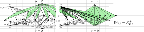
(b) The graph $W_{3,2}$. The seven green shaded regions are copies of $W_{3,1}$.

Figure 3: Illustration for the construction of graphs $W_{i,h}$. Pole vertices are white filled.

(Case $\mathbf{s>1}$). In our proof, we will exploit special graphs $W_{i,h}$, with $1\leq h<i$, having two designated vertices $\nu$ and $\sigma$, called poles; specifically, $\nu$ is the north pole and $\sigma$ is the south pole of $W_{i,h}$; refer to Fig. 3. In the following, we denote by $K^{+}_{2,\alpha}$ the graph obtained from the complete bipartite graph $K_{2,\alpha}$ by adding an edge between the two vertices $t$ and $b$ of the size-$2$ bipartition class of the vertex set of $K_{2,\alpha}$. We say that $t$ and $b$ are the extremes of $K^{+}_{2,\alpha}$, and we refer to $t$ and to $b$ are the top and the bottom extreme, respectively. For any $i\geq 2$, the graphs $W_{i,h}$ are defined as follows. We distinguish based on the value of $h$. If $h=1$, the graph $W_{i,1}$ coincides with $K^{+}_{2,2i+1}$; see Fig. 3(a). If $h>1$, the graph $W_{i,h}$ is obtained from $K^{+}_{2,2i+1}$ by removing each edge $(t,x)$, with $x\neq b$, and by identifying $t$ and $b$ with the north and south pole of a copy of $W_{i,h-1}$, respectively; see Fig. 3(b). We have the following claims.

Claim 5.

For any $i\geq 2$, the graph $W_{i,h}$ admits a leveled planar drawing with span $h+1$ in which the north pole of $W_{i,h}$ lies strictly above all the other vertices of $W_{i,h}$ and the south pole of $W_{i,h}$ lies strictly below all the other vertices of $W_{i,h}$.

Proof.

Figure 4: Example for the construction of the drawings of $W_{i,h}$ that satisfy Claim 5, with $i=3$ and $h=2$. (Left) Initialization of the drawing of $W_{3,2}$ to a straight-line planar drawing of $K^{+}_{2,7}$. (Right) Replacement of the edges $(\nu,x)$, with $x\neq\sigma$, with a drawing of $W_{3,1}$. For readability purposes, only one edge has been replaced with a drawing of $W_{3,1}$; the other replacements are represented by tailed regions.

We prove the statement by induction on $h$; refer to Fig. 4. In the base case $h=1$, and thus $i\geq 2$. Then, $W_{i,1}=K^{+}_{2,2i+1}$, which admits a level planar drawing with span $h+1=2$ with the desired properties; see Fig. 3(a). In the inductive case $h>1$. Then, a drawing $\Gamma$ of $W_{i,h}$ with the desired properties can be constructed as follows. We initialize $\Gamma$ to a straight-line planar drawing of $K^{+}_{2,2i+1}$ in which $\sigma$ is placed on point $(0,0)$, $\mu$ is placed on point $(0,h+1)$, and the remaining $2i+1$ vertices of $K^{+}_{2,2i+1}$ are placed on points $(j,1)$, for $j=1,\dots,2i+1$; see Fig. 4(left). Observe that, in $\Gamma$, the edge $(\mu,\sigma)$ has span $h+1$, the edges incident to $\sigma$ and not to $\mu$ have span $1$, and the edges incident to $\mu$ and not to $\sigma$ have span $h$. We call the latter edges long. By induction, the graph $W_{i,h-1}$ admits a leveled planar drawing $\Gamma^{\prime}$ with span $h$ in which the north pole of $W_{i,h-1}$ lies strictly above all the other vertices of $W_{i,h-1}$ and the south pole of $W_{i,h-1}$ lies strictly below all the other vertices of $W_{i,h-1}$. Consider the leveling $\ell^{\prime}$ of $W_{i,h-1}$ determined by the $y$-coordinates of the vertices in $\Gamma^{\prime}$. W.l.o.g., we assume that $\ell^{\prime}$ assigns the north and the south pole of $W_{i,h-1}$ to levels $h+1$ and $1$, respectively. This allows us to replace the drawing of each long edge $(\mu,x)$ (where $x\neq\sigma$ is the south pole of some copy of $W_{i,h-1}$) with a drawing of $W_{i,h-1}$ in which (i) the north pole of $W_{i,h-1}$ lies upon $\mu$ and the south pole of $W_{i,h-1}$ lies upon $x$, and (ii) the vertices of $W_{i,h-1}$ in level $i$ lie arbitrarily close to the intersection point of $(\mu,x)$ and the level $i$, and so that these vertices are consecutive along level $i$ and have the same left-to-right ordering in the resulting drawing as in $\Gamma^{\prime}$. This yields a leveled planar drawing $\Gamma$ of $W_{i,h}$ with the desired properties. In particular, the span of $\Gamma$ coincides with the span of the edge $(\mu,\nu)$, which is $h+1$. ∎

Claim 6.

For any $i\geq 2$, in any weakly leveled planar drawing of $W_{i,i-1}$ with span at most $i$, the edge connecting the poles of $W_{i,i-1}$ has span $i$.

Proof.

We start by establishing the following two useful properties of any weakly leveled planar drawing $\Gamma^{*}$ with span at most $i$ of $K^{+}_{2,2i+1}$.

P1: In $\Gamma^{*}$, the extremes of $K^{+}_{2,2i+1}$ lie on different levels.

P2: In $\Gamma^{*}$, there exists a vertex $x$ of $K^{+}_{2,2i+1}$ that lies strictly between the extremes of $K^{+}_{2,2i+1}$.

We prove P1. Similarly as in the proof of Property 3.3, if the extremes of $K^{+}_{2,2i+1}$ are assigned to the same level, then by the pigeonhole principle and since $\operatorname{span}(\ell)\leq i$, there must exist two vertices $a$ and $b$ of the above $K^{+}_{2,2i+1}$ that are assigned to a same level. However, the $4$-cycle formed by $a$, $b$, and the two extremes of $K^{+}_{2,2i+1}$ does not admit a level planar drawing with the described level assignment.

We prove P2. Suppose, for the sake of a contradiction, that in $\Gamma^{*}$ no vertex of $K^{+}_{2,2i+1}$ lies strictly between the extremes $t$ and $b$ of $K^{+}_{2,2i+1}$. We call non-extremal the vertices of $K^{+}_{2,2i+1}$ different from $t$ and $b$. Let $\ell^{*}$ be the leveling of $K^{+}_{2,2i+1}$ determined by $\Gamma^{*}$, and assume, w.l.o.g., that $\ell(t)>\ell(b)$. By hypothesis, $\ell^{*}$ assigns each non-extremal vertex $v$ of $K^{+}_{2,2i+1}$ to a level $\ell(v)$ such that either $\ell(v)\leq\ell(b)$ or $\ell(v)\geq\ell(t)$. However, since $\ell(t)-\ell(b)\geq 1$ by P1 and since $|\ell(v)-\ell(t)|\leq i$ and $|\ell(v)-\ell(b)|\leq i$ given that $\Gamma^{*}$ has span at most $i$, there exists at most $i$ levels above and including $\ell(t)$ and at most $i$ levels below and including $\ell(b)$ where $v$ may lie in $\Gamma^{*}$. This defines at most $2i$ available levels for the non-extremal vertices of $K^{+}_{2,2i+1}$. However, since in $\Gamma^{*}$ the vertices $t$ and $b$ lie on different levels, the planarity of $\Gamma^{*}$ enforces that at most two non-extremal vertices of $K^{+}_{2,2i+1}$ can lie on the same level in $\Gamma^{*}$. Since there exist $2k+1$ non-extremal vertices, we get a contradiction.

Consider a weakly leveled planar drawing $\Gamma$ of $W_{i,i-1}$ with span at most $i$ and let $\ell$ be the corresponding leveling. Since $\nu$ and $\sigma$ are the extremes of a $K^{+}_{2,2i+1}$ subgraph of $W_{i,i-1}$, we derive the following. By P2, we have that in $\Gamma$ there exists a vertex $x$ of $W_{i,i-1}$ that lies strictly between the levesl of $\nu$ and $\sigma$. In particular, it holds that $|\ell(\nu)-\ell(x)|\geq 1$ and that $|\ell(\sigma)-\ell(x)|\geq 1$. In turn, this and the fact that $|\ell(\nu)-\ell(\sigma)|=|\ell(\nu)-\ell(x)|+|\ell(\sigma)-\ell(x)|$ imply that $|\ell(\nu)-\ell(\sigma)|\geq|\ell(\nu)-\ell(x)|+1$. Observe now that $\mu$ and $x$ are the poles of a subgraph $=W_{i,i-2}$ of $W_{i,i-1}$, and thus they are also the extremes of a $K^{+}_{2,2i+1}$ subgraph of $W^{\prime}$. Therefore, again by P2, we have that there exists a vertex $x^{\prime}$ of $W^{\prime}$ that lies strictly between the levels of $\nu$ and $x$. In particular, we get that $|\ell(\nu)-\ell(x)|\geq|\ell(\nu)-\ell(x^{\prime})|+1$, which implies that $|\ell(\nu)-\ell(\sigma)|\geq|\ell(\nu)-\ell(x^{\prime})|+2$. The repetition of this argument and the construction of $W_{i,i-1}$ imply that $|\ell(\mu)-\ell(\sigma)|\geq|\ell(\nu)-\ell(x^{*})|+(i-1)$, where $x^{*}$ is a vertex of the “inner most” copy of $K^{+}_{2,2i+1}$ incident to $\nu$. The fact that $|\ell(\nu)-\ell(x^{*})|\geq 1$ implies the statement. ∎

The reduction for $s>1$ is similar to the one for $s=1$, but the role of $K_{2,4}$ is now played by $W_{s,s-1}$. Starting from a bipartite planar graph $H$, we construct a graph $G$ that is a positive instance of $s$-Span Weakly Leveled Planarity if and only if $H$ is a positive instance of $1$-Span Leveled Planarity. To this aim, we proceed as follows. We initialize $G=H$. Then, for each edge $(u,v)$ of $H$, we remove $(u,v)$ from $G$, introduce a copy of $W_{s,s-1}$, which we denote as $W_{s}(u,v)$, and identify $u$ and $v$ with the poles $\nu$ and $\sigma$ of $W_{s,s-1}$, respectively. Clearly, $G$ is planar and the above reduction can be carried out in polynomial time, since the size of $W_{s,s-1}$ depends only on $s$.

Suppose that $H$ admits a leveling $\ell_{H}$, with $\operatorname{span}(\ell_{H})\leq 1$, such that $(H,\ell_{H})$ is level planar, and let $\Gamma_{H}$ be a level planar drawing of $(H,\ell_{H})$. Then, the leveling $\ell^{\prime}_{H}$ of $H$ where $\ell^{\prime}_{H}(v)=s\cdot\ell_{H}(v)$ is clearly such that $(H,\ell^{\prime}_{H})$ is level planar and $\operatorname{span}(\ell^{\prime}_{H})\leq s$. In fact, a level planar drawing $\Gamma^{\prime}_{H}$ of $(H,\ell^{\prime}_{H})$ can be obtained by simply setting the $y$-coordinate of each vertex $v$ in $\Gamma^{\prime}_{H}$ to be $s$ times the $y$-coordinate of $v$ in $\Gamma_{H}$.

By Claim 5, for each edge $(u,v)$ of $H$, there exists a leveled planar drawing $\Gamma_{(u,v)}$ of the graph $W_{s}(u,v)$ with span $s$ in which $u$ lies strictly above all the other vertices of $W_{s}(u,v)$ and $v$ lies strictly below all the other vertices of $W_{s}(u,v)$. Note that, by Claim 6, the span of the edge $(u,v)$ in $\Gamma_{(u,v)}$ is exactly $s$. Let $\ell_{W}$ be the leveling of $W_{s}(u,v)$ determined by the $y$-coordinates of the vertices in $\Gamma_{(u,v)}$. W.l.o.g, we assume that $\ell_{W}(v)=\ell^{\prime}_{H}(v)$.

By construction, each edge $(u,v)$ of $H$ has span $s$ in $\Gamma^{\prime}_{H}$. This and the properties of $\Gamma_{(u,v)}$ listed above allow us to replace the drawing of each edge $(u,v)$ in $\Gamma^{\prime}_{H}$ with a drawing of $\Gamma_{(u,v)}$ in which (i) the placement of $u$ and $v$ is the same as in $\Gamma^{\prime}_{H}$, and (ii) the vertices of $W_{s}(u,v)$ in level $i$ lie arbitrarily close the intersection point in $\Gamma^{\prime}_{H}$ of the edge $(u,v)$ and level $i$, and so that these vertices are consecutive along level $i$ and have the same left-to-right ordering in the resulting drawing as in $\Gamma_{(u,v)}$. This yields a leveled planar drawing $\Gamma_{G}$ of $G$ with span $s$. In fact, if we subdivide each edge of $G$ with span larger than $1$ with a dummy vertex at its intersection with a level in $\Gamma_{G}$, we obtain a drawing and a proper leveling satisfying Section 2).

Suppose now that $G$ admits a leveling $\ell_{G}$, with $\operatorname{span}(\ell_{G})\leq s$, such that $(G,\ell_{G})$ is weakly level planar. We show that $H$ admits a leveling $\ell_{H}$, with $\operatorname{span}(\ell_{H})\leq 1$, such that $(H,\ell_{H})$ is level planar. Let $\Gamma_{G}$ be a straight-line level planar drawing of $(G,\ell_{G})$; in this respect, observe that, a level planar drawing is $y$-monotone, and thus it can be “stretched” into a straight-line planar drawing keeping the $y$-coordinate of the vertices unchanged [DBLP:conf/gd/Biedl14, DBLP:conf/gd/EadesFL96, DBLP:journals/algorithmica/EadesFLN06, DBLP:journals/jgt/PachT04]. Observe that, by construction, $H$ is an induced subgraph of $G$, i.e., $H=G[V(H)]$. Let $\ell^{\prime}_{H}$ be the restriction of $\ell_{G}$ to the vertices of $H$. Recall that, each edge $(u,v)$ of $H$ appears in $G$ as the intra-pole edge of the graph $W_{s}(u,v)$. By Claim 6, we have that $\ell_{G}(u,v)=s$ for any edge $(u,v)$ of $H$. Therefore, the drawing $\Gamma^{\prime}_{H}$ of $H$ contained in $\Gamma_{G}$ is a level planar drawing of $(H,\ell^{\prime}_{H})$, in which each edge has span exactly $s$. It follows immediately that the leveling $\ell_{H}$ of $H$ such that $\ell_{H}(v)=\frac{\ell_{G}(v)}{s}$ is such that $\ell_{H}$ is proper and $(H,\ell_{H})$ is level planar. In fact, a straight-line level planar drawing $\Gamma_{H}$ of $(H,\ell_{H})$ can be obtained from $\Gamma^{\prime}_{H}$ by simply placing each vertex $v$ at a point whose $x$-coordinate is the $x$-coordinate of $v$ in $\Gamma^{\prime}_{H}$ and whose $y$-coordinate is the $y$-coordinate of $v$ in $\Gamma^{\prime}_{H}$ divided by $s$.

The proof of LABEL:thm:np-hardness also shows that, for any fixed $s\geq 1$, deciding whether a graph admits a (non-weakly) leveled planar drawing with span at most $s$ is NP-complete, which generalizes the NP-completeness result by Heath and Rosenberg [DBLP:journals/siamcomp/HeathR92], which is limited to $s=1$.

4 Parameterized Complexity

Motivated by the NP-hardness of the $s$-Span Weakly leveled planarity problem (LABEL:thm:np-hardness), we consider the parameterized complexity of the problem. Recall that a problem $\mathcal{P}$ whose input is an $n$-vertex graph $G$ is fixed-parameter tractable (for short, FPT) with respect to some parameter $k$ if it can be solved via an algorithm with running time $O(f(k)\cdot p(n))$, where $f$ is a computable function and $p$ is a polynomial function. A kernelization for $\mathcal{P}$ is an algorithm that constructs in polynomial time (in $n$) an instance $(G^{\prime},k^{\prime})$, called kernel, such that: (i) the size of the kernel, i.e., the number of vertices in $G^{\prime}$, is some computable function of $k$; (ii) $(G^{\prime},k^{\prime})$ and $(G,k)$ are equivalent instances; and (iii) $k^{\prime}$ is some computable function of $k$. If $\mathcal{P}$ admits a kernel w.r.t. some parameter $k$, then it is FPT w.r.t. $k$.

Theorem 4.1.

cor:fpt-vc Let $(G,s)$ be an instance of $s$-Span Weakly leveled planarity with a vertex cover $C$ of size $k$. There exists a kernelization that applied to $(G,s)$ constructs a kernel of size $O(k^{2})$. Hence, the problem is FPT with respect to the size of a vertex cover.

Proof sketch.

First, we give a kernel (with respect to a parameterization by $k$ and $s$) of size $O(k\cdot s)$. Second, we show that any planar graph $G$ with vertex cover number $k$ admits a weakly leveled planar drawing with span at most $3k$, which allows us to assume $s\leq 3k$.

For the kernel with respect to $k+s$, we follow a classical reduction approach. By planarity, the number of vertices of $G-C$ with three or more neighbors in $C$ can be bounded by $2k$ (e.g., using [flsz-ktpp-19, Lemma 13.3]), and the number of pairs from $C$ with a degree-$2$ neighbor in $G-C$ is at most $3k$. For each vertex $c\in C$ with more than three degree-$1$ neighbors in $G-C$, we only keep three of such neighbors. Then in any drawing of the reduced instance, a neighbor $v_{c}$ of $c$ is not on the same level as $c$, and thus we can reinsert the removed vertices next to $v_{c}$. Also, for each pair of vertices $\{c,d\}\in C$ that are common neighbors of more than $4s+5$ degree-$2$ vertices in $G-C$, we only keep $4s+5$ of such degree-$2$ vertices. Then in any drawing of the reduced instance with span at most $s$, a neighbor $v_{cd}$ of $c$ and $d$ lies strictly between the levels of $c$ and $d$, and thus we can reinsert the removed vertices next to $v_{cd}$. As these reductions can be performed in polynomial time, this yields a kernel of size $O(k\cdot s)$.

To bound the span, we consider a more strict trimming operation that removes all degree-$1$ vertices of $G-C$ and replaces all degree-$2$ vertices of $G-C$ with the same two neighbors $u,v\in C$ by a single edge $(u,v)$. As above, the size of this trimmed graph is $O(k)$. It therefore admits a planar leveled drawing of height (and thus also span) $O(k)$, into which the removed vertices can be inserted without asymptotically increasing the height. ∎

Proof 4.2.

The kernel $(G^{\prime},s)$ is obtained as in LABEL:thm:kernel-cover-span, by applying LABEL:rule:vc-deg1 and LABEL:rule:vc-deg2, however, for each pair of vertices $\{c,d\}\in C$, the number of degree-$2$ vertices of $G$ that are neighbors of $c$ and $d$ and that are kept in the kernel is at most $24k+5$. Since this number is in $O(k)$ and since the number of pairs of vertices $\{c,d\}\in C$ such that $c$ and $d$ are the neighbors of a degree-$2$ vertex in $V-C$ is also in $O(k)$ by LABEL:le:degree-3-vc, the bound on the kernel size follows from the one of LABEL:thm:kernel-cover-span. Since the kernel can be constructed in polynomial time, it follows that $s$-Span Weakly leveled planarity is FPT with respect to $k$.

It remains to prove that $(G^{\prime},s)$ is equivalent to $(G,s)$. The proof distinguishes two cases. If $s\leq 6k$, then the proof follows from LABEL:thm:kernel-cover-span, as in this case $(G^{\prime},s)$ is the same kernel as the one computed for that theorem. On the other hand, if $s>6k$, as proved previously $(G,s)$ is a positive instance, and hence $(G^{\prime},s)$ is a positive instance, as well.

Let $(G,s)$ be an instance of $s$-Span Weakly leveled planarity and $b$ be a parameter. A set $M$ of vertices of $G$ is a modulator to components of size $b$ ($b$-modulator for short) if every connected component of $G-M$ has size at most $b$. Note that a $1$-modulator is a vertex cover. We show that testing whether a graph with a $b$-modulator of size $k$ admits a weakly leveled planar drawing with span $s$ is FPT w.r.t. $b+k$. The neighbors in $M$ of a component $C$ of $G-M$ are its attachments, and are denoted by $\mathrm{att}(C)$. We also denote by $\mathrm{bridge}(C)$ the graph consisting of $C$, $\mathrm{att}(C)$, and the edges between $C$ and its attachments.

We generalize the technique for vertex cover and give a kernel with respect to $b+k+s$ and further show that any planar graph admits a leveled planar drawing with height (and hence span) bounded by $(5b+1)bk$. Hence, $s$ can be bounded by a function of $b+k$, which yields the result. Differently from vertex cover, the components of $G-M$ are not single vertices but have up to $b$ vertices. Nevertheless, we use planarity to bound the number of components with three or more attachments by $2k$ and the number of pairs $\{u,v\}\in M$ that are the attachments of components of $G-M$ by $3k$. The most challenging part is again dealing with the components of $G-M$ with one or two attachments, as their number might not be bounded by any function of $b+k$. Here, the key insight is that, since these components have size at most $b$, there is only a bounded number of “types” of these components. More precisely, two components $C_{1},C_{2}$ of $G-M$ that have the same attachments are called equivalent if there is an isomorphism between $\mathrm{bridge}(C_{1})$ and $\mathrm{bridge}(C_{2})$ that leaves the attachments fixed. We use the fact that there is a computable (in fact exponential, see e.g. [DBLP:journals/jct/ChapuyFGMN11]) function $f\colon\mathbb{N}\to\mathbb{N}$ such that the number of equivalence classes is bounded by $f(b)$.

We can show that if an equivalence class of components with one attachment (with two attachments) is sufficiently large, that is, it is at least as large as a suitable function of $s$ and $b$, then in any leveled planar drawing with bounded span, one such component must be drawn on levels that are all strictly above or all strictly below its attachment (resp. on levels that are strictly between its two attachments). Then arbitrarily many equivalent components can be inserted into a drawing without increasing its span. This justifies the following reduction rules.

Rule 1.

For every vertex $v\in M$, let $\mathcal{C}_{v}$ be a set containing all and only the equivalent components $C$ of $G-M$ such that $\mathrm{att}(C)=\{v\}$. If $|\mathcal{C}_{v}|>(4s+4)b$, then remove all but $(4s+4)b$ of these components from $G$.

Rule 2.

For every pair of vertices $\{u,v\}\in M$, let $\mathcal{C}_{uv}$ be a set containing all and only the equivalent components $C$ of $G-M$ with $\mathrm{att}(C)=\{u,v\}$. If $|\mathcal{C}_{uv}|>(8s+8)(b+1)$, then remove all but $(8s+8)(b+1)$ such components from $G$.

We can now sketch a proof of the following theorem.

Theorem 4.3.

cor:kernel-modulator-span Let $(G,s)$ be an instance of $s$-Span Weakly leveled planarity with a $b$-modulator of size $k$. There exists a kernelization that applied to $(G,s)$ constructs a kernel of size $O(f(b)\cdot k^{2}\cdot b^{4})$. Hence, the problem is FPT with respect to $k+b$.

Proof sketch.

As mentioned above, the number of components of $G-M$ with three or more attachments is at most $2k$. Rules 1 and 2 bound the number of equivalent components with one and two attachments. The fact that the number of equivalence classes is bounded by $f(b)$ then yields a kernel of size $O(f(b)\cdot k\cdot b^{2}\cdot s)$. Note that testing whether two components are equivalent can be reduced to an ordinary planar graph isomorphism problem [DBLP:conf/stoc/HopcroftW74], by connecting each attachment to a sufficiently long path, which forces the isomorphism to leave the attachments fixed. Hence, the described reduction can be performed in polynomial time.

To drop the dependence on $s$ of the kernel size, we prove that every planar graph admits a leveled planar drawing whose height (and hence span) is at most $(5b+1)bk$. To this end, we use a trim operation that removes all components of $G-M$ with a single attachment and replaces multiple components of $G-M$ with attachments $\{u,v\}$ by a single edge $(u,v)$. The size of the trimmed graph is at most $(5b+1)k$, therefore there exists a leveled planar drawing of the trimmed graph whose span is bounded by the same function. Then the removed components, which have size at most $b$, can be reinserted by introducing $b$ new levels below each level, i.e., the span increases by a linear factor in $b$. This yields the desired leveled planar drawing with span at most $(5b+1)bk$ and thus a kernel of the claimed size. ∎

Proof 4.4.

The kernel $(G^{\prime},s)$ is obtained as in LABEL:thm:kernel-modulator-span, by applying Rules 1 and 2, however:

• for each vertex $u\in M$, the number of components with attachment $\{u\}$ that belong to each equivalence class and that are kept in the kernel is at most $(4((5b+1)\cdot b\cdot k)+4)\cdot b$; and

• for each pair of vertices $\{u,v\}\in M$, the number of components with attachments $\{u,v\}$ that belong to each equivalence class and that are kept in the kernel is at most $(8((5b+1)\cdot b\cdot k)+8)\cdot(b+1)$.

Since the number of equivalence classes is at most $f(b)$, the number of vertices in each component is at most $b$, and the number of pairs of vertices $\{u,v\}\in M$ that are attachment to some component of $G-M$ is in $O(k)$ by LABEL:le:degree-3-vc, it follows that the size of the kernel is $O(f(b)\cdot k^{2}\cdot b^{4})$. Since the kernel can be constructed in polynomial time, as proved in LABEL:thm:kernel-modulator-span, it follows that $s$-Span Weakly leveled planarity is FPT with respect to $k$.

It remains to prove that $(G^{\prime},s)$ is equivalent to $(G,s)$. The proof distinguishes two cases. If $s\leq(5b+1)\cdot b\cdot k$, then the proof follows from LABEL:thm:kernel-cover-span, as in this case $(G^{\prime},s)$ is the same kernel as the one computed for that theorem. On the other hand, if $s>(5b+1)\cdot b\cdot k$, by LABEL:lem:bm-span-bound, we have that $(G,s)$ is a positive instance, and hence $(G^{\prime},s)$ is a positive instance, as well.

We now move to treedepth. A treedepth decomposition of a graph $G=(V,E)$ is a tree $T$ on vertex set $V$ with the property that every edge of $G$ connects a pair of vertices that have an ancestor-descendant relationship in $T$. The treedepth of $G$ is the minimum depth (i.e., maximum number of vertices in any root-to-leaf path) of a treedepth decomposition $T$ of $G$.

Let $td$ be the treedepth of $G$ and $T$ be a treedepth decomposition of $G$ with depth $td$. Let $r$ be the root of $T$. For a vertex $u\in V$, we denote by $T_{u}$ the subtree of $T$ rooted at $u$, by $V_{u}$ the vertex set of $T_{u}$, by $d(u)$ the depth of $u$ (where $d(u)=1$ if $u$ is a leaf and $d(u)=td$ if $u=r$), and by $R(u)$ the set of vertices on the path from $u$ to $r$ (end-vertices included).

As for LABEL:cor:fpt-vc and LABEL:cor:kernel-modulator-span, we can show that the instance $(G,s)$ is positive if $s$ is sufficiently large, namely larger than $((5td)^{td}+1)^{td}$. Hence, we can assume that $s$ is bounded w.r.t. $td$.

Theorem 4.5.

th:drawing-treedepth Every planar graph with treedepth $td$ has a leveled planar drawing of height at most $((5td)^{td}+1)^{td}$.

Proof sketch.

We apply a trimming operation similar to the one described in LABEL:cor:kernel-modulator-span. The effect of this operation, when applied to a vertex $v$, is to bound the number of children of $v$ in $T$ by $5td$. Assume that every vertex in $V_{v}\setminus\{v\}$ has at most $5td$ children. Then $R(v)$ is a vertex set of size at most $td$ and, due to the degree bound, any connected component of $G-R(v)$ whose vertices are in $V_{v}$ has size bounded by $(5td)^{td}$. Similarly as for modulators, we can remove such components with a single attachment and replace multiple components with the same two attachments by an edge. This bounds the degree of $v$ in $T$ to $5td$ ($2td$ for components with three or more attachments and $3td$ for components with two attachments).

We apply this trimming operation in batches. The first batch processes all leaves (which has no effect); each next batch consists of all the vertices whose children are already processed. After at most $td$ batches the whole tree is processed (and in fact reduced to a single vertex by processing the root). We then undo these steps while maintaining a leveled planar drawing. The key point here is that, due to the degree bound, each of the removed components contains at most $(5td)^{td}$ vertices, and we can simultaneously reinsert all removed components at the cost of inserting $(5td)^{td}$ levels below each existing level in the current drawing. Therefore, the number of levels multiplies by $(5td)^{td}+1$ per batch. ∎

Proof 4.6.

We first defined a trimmed graph from $G$ (and a corresponding treedepth decomposition from $T$). The trimming operation we define in order to get the trimmed graph is similar to the one defined in LABEL:subse:fpt-mbsc. However, it is applied $td+1$ times, namely for increasing values of $i$ from $1$ to $td$, it is applied to all the vertices of $G$ that have depth $i$ in $T$. The main feature of the trimming operation is that, for each processed vertex $v$ of $G$, the outdegree (that is, the number of children) of $v$ in $T$ is bounded by $5td$.

Vertices at depth $0$ already satisfy this property initially. Let $v$ be a non-processed vertex at depth $j$ whose children $u_{1},\dots,u_{k}$ have been already processed. We process $v$ as follows. By the defining property of a treedepth decomposition, each connected component of $G-R(v)$ is such that its vertex set is either part of $V_{u_{i}}$, for some $i\in\{1,\dots,k\}$, or is disjoint from $V_{v}$. Let $\mathcal{C}$ denote the set of connected components of $G-R(v)$ whose vertex sets are contained in the sets $V_{u_{1}},\dots,V_{u_{k}}$. We remove all components in $\mathcal{C}$ with one attachment and, if there are two or more distinct components in $\mathcal{C}$ with the same two attachments $\{s,t\}$, we replace all such components with a single edge $(s,t)$. By LABEL:le:degree-3-vc, there are at most $3td$ pairs $\{s,t\}$ such that $\mathcal{C}$ contains a component whose attachment is $\{s,t\}$. Furthermore, again by LABEL:le:degree-3-vc, there are at most $2td$ components in $\mathcal{C}$ with three or more attachments in $R(v)$. Henceforth, the number of components in $\mathcal{C}$ that survive the trimming operation is at most $5td$. This is also an upper bound on the size of the outdegree of $v$ in $T$.

Let $(G_{0},T_{0}):=(G,T)$. For $j=1,\dots,td$, we define $(G_{j},T_{j})$ to be the graph obtained from $(G_{j-1},T_{j-1})$ by processing all vertices at depth $j$ as described above. We claim that in $(G_{j},T_{j})$ all vertices at depth $j$ or less have outdegree at most $5td$ in $T_{j}$. This clearly holds for $(G_{0},T_{0})$, since leaves have outdegree $0$. Furthermore, the described processing of vertices at depth $j$ ensures that the claim holds for $(G_{j},T_{j})$ given that it holds for $(G_{j-1},T_{j-1})$.

Note that, by construction, the graph $G_{td}$ consists of a single vertex, given that $R(r)$ consists just of the root $r$ and no component of $G-R(r)$ with one attachment is kept in $G_{td}$ by the trimming operation. Therefore, $G_{td}$ has a leveled planar drawing with height $1$. Similarly to LABEL:lem:bm-span-bound, we show that, given a leveled planar drawing of $G_{i}$ with height $h$, we can construct a leveled planar drawing of $G_{i-1}$ of height $h((5td)^{td}+1)$. This then implies a drawing of $G=G_{0}$ of height $((5td)^{td}+1)^{td}$, as desired.

Let $\Gamma_{i}$ be a leveled planar drawing of $G_{i}$ with height $h$. To obtain a leveled planar drawing $\Gamma_{i-1}$ of $G_{i-1}$, we insert $(5td)^{td}$ levels immediately below every level of $\Gamma_{i}$ (thus, the number of levels of $\Gamma_{i-1}$ is $h((5td)^{td}+1)$). We use these levels to re-insert the components of $G_{i-1}$ that were removed to obtain $G_{i}$. This is done as follows. Let $C$ be one of such components and let $v$ be the vertex whose processing (in $T_{i-1}$) led to the removal of $C$. By assumption, all vertices in $V_{v}\setminus\{v\}$ have outdegree at most $5td$ in $T_{i-1}$ and therefore the number of vertices in $C$ is at most $(5td)^{td}$. If $C$ has a single attachment $x\in R(v)$, by LABEL:lem:1-att-drawing, we obtain a leveled planar drawing $\Gamma_{C}$ of $C$ together with its attachment on $(5td)^{td}+1$ levels in which $x$ is the unique vertex on the highest level. Note that $x$ belongs to $\Gamma_{i}$. We can thus use the level of $x$ and the $(5td)^{td}$ new levels immediately below it to merge $\Gamma_{C}$ into $\Gamma_{i}$ (by merging the two copies of $x$). If $C$ has two attachments $x,y\in R(v)$, then $G_{i}$ contains the edge $(x,y)$. By LABEL:lem:2-att-drawing, we have that $C$ together with $x,y$ have a leveled planar drawing $\Gamma_{C}$ on $(5td)^{t}d+2$ levels, where $x$ and $y$ are the unique vertices on the highest and the lowest level, respectively. Note that $x$ and $y$ belong to $\Gamma_{i}$. As $x$ and $y$ are drawn on distinct levels in $\Gamma_{i}$, there are $(5td)^{t}d$ new intermediate levels between them, and we can merge the drawing of $C\cup\{x,y\}$ into $\Gamma_{i}$ next to $(x,y)$ (by merging the two copies of $x$ and the two copies of $y$, respectively). By reinserting all components in this way, we obtain a leveled planar drawing $\Gamma_{i-1}$ of $G_{i-1}$ with height $h((5td)^{td}+1)$.

We thus obtain the following.

Theorem 4.7.

thm:treedepth-FPT Let $(G,s)$ be an instance of $s$-Span Weakly leveled planarity with treedepth $td$. There exists a kernelization that applied to $(G,s)$ constructs a kernel whose size is a computable function of $td$. Hence, the problem is FPT with respect to the treedepth.

Proof sketch.

We perform a kernelization with respect to $td+s$. We then apply LABEL:th:drawing-treedepth to bound the span in terms of treedepth. We use a strategy similar to the one in LABEL:th:drawing-treedepth for processing the vertices in $td$ batches. However, instead of the trimming operation used there, we use Rules 1 and 2 to bound, for each vertex $v$, the number of components of $G-R(v)$ whose vertices are in $V_{v}$ by a function $g(td,s)$. Eventually, we obtain an equivalent instance in which the vertices have their degree bounded by $g(td,s)$ in $T$. This is the desired kernel. ∎

5 Upper and Lower Bounds

In this section, we establish upper and lower bounds on the span of weakly leveled planar drawings of certain graph classes.

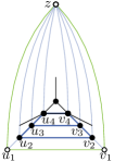
(a)

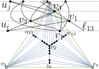
(b)

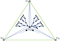
(c)

Figure 5: (a) A $n$-vertex $2$-outerplanar graph requiring $\Omega(n)$ span in every weakly leveled planar drawing. (b) An $n$-vertex $3$-connected cycle-tree requiring span $4$ in every weakly leveled planar drawing. (c) An $n$-vertex cycle-tree requiring $\Omega(\log n)$ span in every weakly leveled planar drawing. The graph resulting from the removal of the vertices incident to the outer face is drawn bold.

Theorem 5.1.

thm:2-outerplanar There exists an $n$-vertex $2$-outerplanar graph such that every weakly leveled planar drawing of it has span in $\Omega(n)$.

Proof sketch.

The lower bound is provided by the graph $G_{k}$ of Fig. 5(a), which is composed of $k:=\lfloor(n-1)/2\rfloor$ “$1$-fused stacked cycles” and introduced by Biedl [DBLP:journals/dcg/Biedl11]. It is easy to observe that each cycle has an edge that spans two more levels than any edge of a cycle stacked inside it, from which the linear lower bound follows. ∎

Proof 5.2.

Suppose first that $n$ is odd. The lower bound is provided by the graph $G_{k}$ composed of $k:=\lfloor(n-1)/2\rfloor$ “$1$-fused stacked cycles” (see Fig. 5(a)): Start from $k$ cycles $\mathcal{C}_{i}:=(u_{i},v_{i},z_{i})$, identify vertices $z_{1},\dots,z_{k}$ into a unique vertex $z$, and insert the edges of the paths $(u_{1},\dots,u_{k})$ and $(v_{1},\dots,v_{k})$. Biedl [DBLP:journals/dcg/Biedl11] introduced $G_{k}$ as an example of a $2$-outerplanar graph requiring $\Omega(n)$ width and height in any planar polyline grid drawing. We can use the same inductive proof as hers to show that one of the edges of $\mathcal{C}_{k}$ has a span $k\in\Omega(n)$ in any weakly leveled planar drawing $\Gamma_{k}$ of $G_{k}$ in which the outer face is delimited by $\mathcal{C}_{k}$. If $k=1$, the claim is trivial. If $k>1$, consider the subgraph $G_{k-1}$ of $G_{k}$ induced by $\mathcal{C}_{1},\dots,\mathcal{C}_{k-1}$ and let $\Gamma_{k-1}$ be the restriction of $\Gamma_{k}$ to $G_{k}$. By induction, in $\Gamma_{k-1}$ one of the edges of $\mathcal{C}_{k-1}$, say $e$, has span at least $k-1$. Since $\mathcal{C}_{k}$ surrounds $e$ in its interior in $\Gamma_{k}$, except possibly the vertex $z$ that might be shared by $e$ and $\mathcal{C}_{k}$, it follows that $\mathcal{C}_{k}$ touches at least one more level than $e$, hence the longest edge of $\mathcal{C}_{k}$ has span at least $k$ in $\Gamma_{k}$. Two observations conclude the proof. First, in any weakly leveled planar drawing of $G_{k}$, there is a subgraph with at least $\lceil k/2\rceil\in\Omega(n)$ $1$-fused stacked cycles that is drawn so that these cycles are one nested into the other (this removes the assumption that the outer face has to be delimited by $\mathcal{C}_{k}$). Second, if $n$ is even, we can add to $G_{k}$ a vertex adjacent to $z$ and $u_{1}$; this maintains the graph $2$-outerplanar.

There is however a well-studied graph family, the Halin graphs, which have outerplanarity 2 and admit $1$-span weakly leveled planar drawings [DBLP:journals/algorithmica/BannisterDDEW19, digiacomo2023new]. This motivates the study of cycle-trees [DBLP:conf/isaac/LozzoDEJ17], a superclass of Halin graphs still having outerplanarity 2. We first consider 3-connected cycle-trees showing a constant span and then extend the study to general cycle-trees. The approach for 3-connected cycle-trees relies on removing an edge from the external face so to obtain a graph for which we construct a suitable decomposition tree. We conclude by discussing the span of weakly leveled planar drawings of planar graphs with treewidth 2.

Path-Trees.

A path-tree is a plane graph $G$ that can be augmented to a cycle-tree $G^{\prime}$ by adding the edge $e=(\ell,r)$ in its outer face; see Fig. 6(a). W.l.o.g., let $\ell$ occur right before $r$ in clockwise order along the outer face of $G^{\prime}$; then $\ell$ and $r$ are the leftmost and rightmost path-vertex of $G$, respectively. The external (internal) vertices of $G^{\prime}$ are path-vertices (tree-vertices). The tree-vertices induce a tree in $G$. We can select any tree-vertex $\rho$ incident to the unique internal face of $G^{\prime}$ incident to $e$ as the root of $G$. Then $G$ is almost-$3$-connected if it becomes $3$-connected by adding the edges $(\rho,\ell)$, $(\rho,r)$, and $(\ell,r)$, if they are not already part of $G$. If $G$ is almost-$3$-connected, the path-vertices induce a path in $G$.

(a)

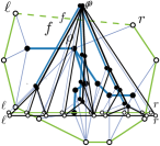
(b)

Figure 6: (a) An almost-3-connected path-tree $G$, drawn with solid edges. The path-vertices are white and the tree-vertices are black. (b) The path-tree $G$ with root $\rho$.

SPQ-decomposition of path-trees.

Let $G$ be an almost-$3$-connected path-tree with root $\rho$, leftmost path-vertex $\lambda$, and rightmost path-vertex $r$. We define the SPQ-decomposition of $G$, introduced in [DBLP:conf/isaac/LozzoDEJ17], which constructs a tree $\mathcal{T}$, called the SPQ-tree of $G$. The nodes of $\mathcal{T}$ are of three types: S-, P-, and Q-nodes. Each node $\mu$ of $\mathcal{T}$ corresponds to a subgraph $G_{\mu}$ of $G$, called the pertinent graph of $\mu$, which is an almost-$3$-connected rooted path-tree. We denote by $\rho_{\mu}$ the root of $G_{\mu}$ (a tree-vertex), by $\lambda_{\mu}$ the leftmost path-vertex of $G_{\mu}$, and by $r_{\mu}$ the rightmost path-vertex of $G_{\mu}$. To handle the base case, we consider as a path-tree also a graph whose path is the single edge $(\lambda,r)$ and whose tree consists of a single vertex $\rho$, possibly adjacent to only one of $\lambda$ and $r$. Also, we consider as almost-$3$-connected a path-tree such that adding $(\rho,r)$, $(\rho,\lambda)$, and $(\lambda,r)$, if missing, yields a $3$-cycle.

We now describe the decomposition.

• Q-node: the pertinent graph $G_{\mu}$ of a Q-node $\mu$ is an almost-$3$-connected rooted path-tree which consists of $\rho_{\mu}$, $\lambda_{\mu}$, and $r_{\mu}$. The edge $(\lambda_{\mu},r_{\mu})$ belongs to $G_{\mu}$, while the edges $(\rho_{\mu},\lambda_{\mu})$ and $(\rho_{\mu},r_{\mu})$ may not exist; see Fig. 7(left).

• S-node: the pertinent graph $G_{\mu}$ of an S-node $\mu$ is an almost-$3$-connected rooted path-tree which consists of $\rho_{\mu}$ and of an almost-$3$-connected path-tree $G_{\nu}$, where $\rho_{\mu}$ is adjacent to $\rho_{\nu}$ and, possibly, to $\lambda_{\nu}$ and $r_{\nu}$. We have that $\mu$ has a unique child in $\mathcal{T}$, namely a node $\nu$ whose pertinent graph is $G_{\nu}$. Further, we have $\lambda_{\mu}=\lambda_{\nu}$ and $r_{\mu}=r_{\nu}$; see Fig. 7(middle).

• P-node: the pertinent graph $G_{\mu}$ of a P-node $\mu$ is an almost-$3$-connected rooted path-tree which consists of almost-$3$-connected rooted path-trees $G_{\nu_{1}},\dots,G_{\nu_{k}}$, with $k>1$. This composition is defined as follows. First, we have $\rho_{\mu}=\rho_{\nu_{1}}=\dots=\rho_{\nu_{k}}$. Second, we have $\lambda_{\nu_{i}}=r_{\nu_{i-1}}$, for $i=2,\dots,k$. Third, $\mu$ has children $\nu_{1},\dots,\nu_{k}$ (in this left-to-right order) in $\mathcal{T}$, where $G_{\nu_{i}}$ is the pertinent graph of $\nu_{i}$, for $i=1,\dots,k$. Finally, we have $\lambda_{\mu}=\lambda_{\nu_{1}}$ and $r_{\mu}=r_{\nu_{k}}$; see Fig. 7(right).

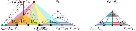
Figure 7: Path-trees corresponding to a Q-node (left), an S-node (middle), and a P-node (right). Dashed edges may or may not belong to $G_{\mu}$. Shaded triangles represent smaller path-trees $G_{\nu_{i}}$.

In the following, all considered SPQ-trees are canonical, that is, the child of every P-node is an S- or Q-node. For a given path-tree, a canonical SPQ-tree always exists [DBLP:journals/algorithmica/ChaplickLGLM24].

3-connected Cycle-Trees.

Let $G$ be a plane graph with three consecutive vertices $u,v,w$ encountered in this order when walking in clockwise direction along the boundary of the outer face of $G$. A leveling of $G$ is single-sink with respect to $(u,v,w)$ if all vertices of $G$ have a neighbor on a higher level, except for exactly one of $\{u,v,w\}$. A single-sink leveling $\ell$ with respect to $(u,v,w)$ is flat if $\ell(u)<\ell(v)<\ell(w)$ or $\ell(w)<\ell(v)<\ell(u)$; $\ell$ is a roof if $\ell(v)>\ell(u)$ and $\ell(v)>\ell(w)$. Note that a single-sink leveling is necessarily either roof or flat.

Given a single-sink leveling $\ell$ of $G$ with respect to $(u,v,w)$, a good weakly leveled planar drawing $\Gamma$ of $(G,\ell)$ is one with the following properties: 1. $\Gamma$respects the planar embedding of $G$; 2. it holds that $x(u)<x(w)$ in $\Gamma$; and 3. all vertices of $V(G)\setminus\{u,v,w\}$ are contained in the interior of the bounded region $R_{uvw}$ defined by the path $(u,v,w)$, by the vertical rays starting at $u$ and $w$, and by the horizontal line $y:=\min_{z\in V(G)}\ell(z)$.

Let $a$ and $b$ be two non-zero integers. A good weakly leveled planar drawing $\Gamma$ of $(G,\ell)$ is an (a,b)-flat drawing if $\ell$ is flat, $a=\ell(v)-\ell(u)$, and $b=\ell(w)-\ell(v)$; it is an (a,b)-roof drawing if $\ell$ is roof, $a=\ell(v)-\ell(u)$, and $b=\ell(w)-\ell(v)$. Note that, by definition, in an $(a,b)$-flat drawing we have that $a$ and $b$ are either both positive or both negative, while in an $(a,b)$-roof drawing $a$ is positive and $b$ is negative.

(a) A $(1,1)$-flat weakly leveled planar drawing when $\mu$ has an odd (left) or even (right) number of children.

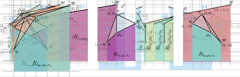
(b) A $(3,1)$-flat weakly leveled planar drawing when $\mu$ has an odd (left) or even (right) number of children.

Figure 8: Illustrations for the proof of LABEL:thm:triconnected-cycle-trees, when $\mu$ is a P-node.

Figure 9: Illustrations for the proof of LABEL:thm:triconnected-cycle-trees, when $\mu$ is a Q-node and the height of $\mathcal{T}$ is $0$.

(a) $(1,1)$-flat

(b) $(3,1)$-flat

(c) $(3,-1)$-roof

Figure 10: Illustrations for the proof of LABEL:thm:triconnected-cycle-trees, when $\mu$ is an S-node.

Theorem 5.3.

thm:triconnected-cycle-trees Every $3$-connected cycle-tree admits a $4$-span weakly leveled planar drawing. Also, for all $n\geq 43$, there exists an $n$-vertex $3$-connected cycle-tree $G$ such that every weakly leveled planar drawing of $G$ has span greater than or equal to $4$.

Proof sketch.

We first prove the statement for almost $3$-connected path trees. Let $G$ be such a graph and $\mathcal{T}$ be its SPQ-tree with root $\mu$. Let $u=\lambda_{\mu}$, $v=\rho_{\mu}$, and $w=r_{\mu}$. Since removing edges does not increase the span of a weakly leveled planar drawing, we can assume that the edges $(u,v)$ and $(v,w)$ belong to $G$ and that $G$ is internally triangulated. That is, we prove the statement when $G$ is a maximal almost-$3$-connected path-tree. The proof is based on recursively constructing a drawing of $G=G_{\mu}$, where the recursion is on the SPQ-tree $\mathcal{T}$ of $G$, according to the following case distinction (for details, see LABEL:lem:triconnected-cycle-paths in the appendix).

If $\mu$ is a P-node, then $G_{\mu}$ has flat levelings $\ell^{i}_{\mu}$ for $i=1,\dots,4$, with $\operatorname{span}(\ell^{i}_{\mu})\leq 4$, such that $(G_{\mu},\ell^{i}_{\mu})$ admits a $p_{i}$-flat weakly leveled planar drawing with $p_{1}=(-1,-1)$, $p_{2}=(1,1)$, $p_{3}=(-1,-3)$, and $p_{4}=(3,1)$, see Fig. 8. Let $k$ be the number of children of $\mu$ in $\mathcal{T}$. Each flat leveling $\ell^{i}_{\mu}$ is obtained by combining roof levelings for the pertinent graphs of the leftmost (or the righmost) $k-1$ children of $\mu$ with a flat leveling of the pertinent graph of the rightmost (resp. leftmost) child of $\mu$. In particular, the $k-1$ children of $\mu$ for which flat levelings are used alternate, in left-to-right order, between $(1,-3)$-roof drawings and $(3,-1)$-roof drawings. If $\mu$ is a Q-node, then $G_{\mu}$ has flat levelings $\ell^{i}_{\mu}$ for $i=1,\dots,4$, with $\operatorname{span}(\ell^{i}_{\mu})\leq 4$, such that $(G_{\mu},\ell^{i}_{\mu})$ admits a $q_{i}$-flat weakly leveled planar drawing with $q_{1}=(1,1)$, $q_{2}=(-1,-1)$, $q_{3}=(3,1)$, and $q_{4}=(-1,-3)$. Also, $G_{\mu}$ has roof levelings $\ell^{j}_{\mu}$ for $j=5,6$, with $\operatorname{span}(\ell^{j}_{\mu})\leq 4$, such that $(G_{\mu},\ell^{j}_{\mu})$ admits a $q_{j}$-roof weakly leveled planar drawing with $q_{5}=(1,-3)$ and $q_{6}=(3,-1)$, see Fig. 9. Finally, if $\mu$ is am S-node, then $G_{\mu}$ has the same type of levelings and weakly leveled planar drawings as in the case in which it is a Q-node, see Fig. 10. Each of such levelings is obtained from a flat leveling of the pertinent graph of the unique child of $\mu$.

For triconnected cycle-trees, we remove an edge $e$ on the outer face, after an augmentation we obtain a $(1,1)$-flat weakly leveled planar drawing, and insert back $e$ with span $2$.

The proof of the theorem is completed by observing that some $3$-connected cycle-trees, like the one in Fig. 5(b), require span at least $4$. ∎

Proof 5.4.

The proof of the theorem immediately follows from LABEL:lem:upper-cycle-tree-3conn and LABEL:lem:lower-cycle-tree-3conn.

The approach in the proof of LABEL:thm:triconnected-cycle-trees can be implemented in quadratic time. To get linear time, we can maintain only the order of the vertices on their levels and calculate the exact coordinates at the end of the algorithm.

Similar to [DBLP:journals/dmtcs/DujmovicPW04, Lemma 14], one can prove that $s$-span weakly leveled planar graphs have queue number at most $s+1$; see LABEL:lem:span-queue in the appendix. Thus, we have the following.

Corollary 5.5.

The queue number of $3$-connected cycle-trees is at most $5$.

The edge-length ratio of a straight-line graph drawing is the maximum ratio between the Euclidean lengths of $e_{1}$ and $e_{2}$, over all edge pairs $(e_{1},e_{2})$. The planar edge-length ratio of a planar graph $G$ is the infimum edge-length ratio of $\Gamma$, over all planar straight-line drawings $\Gamma$ of $G$. Constant upper bounds on the planar edge-length ratio are known for outerplanar graphs [DBLP:journals/tcs/LazardLL19] and for Halin graphs [digiacomo2023new]. We exploit the property that graphs that admit $s$-span weakly leveled planar drawings have planar edge-length ratio at most $2s+1$ [digiacomo2023new, Lemma 4] to obtain a constant upper bound on the edge-length ratio of 3-connected cycle trees.

Corollary 5.6.

The planar edge-length ratio of $3$-connected cycle-trees is at most $9$.

General Cycle-Trees.

We now discuss general cycle-trees, for which we can prove a $\Theta(\log n)$ bound on the span of their weakly leveled planar drawings.

Theorem 5.7.

thm:general-cycle-trees Every $n$-vertex cycle-tree has an $s$-span weakly leveled planar drawing such that $s\in O(\log n)$. Also, there exists an $n$-vertex cycle-tree such that every weakly leveled planar drawing of $G$ has span in $\Omega(\log n)$.

Proof sketch.

For the lower bound, we observe that some cycle-trees require span $\Omega(\log n)$. Indeed, in any planar drawing of the graph in Fig. 5(c), a cycle with $3$ vertices contains a complete binary tree with $\Omega(n)$ vertices in its interior. Then the lower bound on the span follows from the fact that any weakly leveled planar drawing $\Gamma$ of a complete binary tree with $\Omega(n)$ vertices has height $\Omega(\log n)$ (because it has $\Omega(\log n)$ pathwidth [DBLP:journals/tcs/Bodlaender98, scheffler] and the height of $\Gamma$ is lower-bounded by a linear lower function of the pathwidth of the tree [DBLP:journals/algorithmica/DujmovicFKLMNRRWW08]).

For the upper bound, let $G$ be a connected $n$-vertex cycle-tree. Let $\mathcal{E}$ be a plane embedding of $G$ in which the outer face is delimited by a walk $W$, so that removing the vertices of $W$ from $G$ one gets a tree $T$; see Fig. 11(a). We add the maximum number of edges connecting vertices of $W$ with vertices of $W$ and of $T$, while preserving planarity, simplicity, and the property that every vertex of $W$ is incident to the outer face; see Fig. 11(b).

(a)

(b)

(c)

(d)

Figure 11: (a) An embedding $\mathcal{E}$ of a cycle-tree $G$, where the tree $T$ is represented by bold lines. (b) The augmentation of $G$; the added edges are red. The face $f$ of $\mathcal{E}_{G_{W}}$ is gray. (c) Removing the components of $G$ outside $C$. (d) Removing the components of $G$ inside $C$.

We now remove some parts of the graph, so that it turns into a $3$-connected cycle-tree $H$. Let $G_{W}$ be the subgraph of $G$ induced by the vertices of $W$ and let $\mathcal{E}_{G_{W}}$ be the restriction of $\mathcal{E}$ to $G_{W}$. There is a unique face $f$ of $\mathcal{E}_{G_{W}}$ that contains $T$ in its interior; let $C$ be the cycle delimiting $f$. We remove from $G$ the vertices of $G_{W}$ not in $C$. The removed vertices induce connected subgraphs of $G$, called components of $G$ outside $C$; see Fig. 11(c). Also, we remove from $G$ all the vertices of $T$ that have at most one neighbor in $C$. This results in the removal of subtrees of $T$, which we call components of $G$ inside $C$; see Fig. 11(d).

We next apply LABEL:thm:triconnected-cycle-trees to construct a weakly leveled planar drawing $\Lambda$ of $H$ with $O(1)$ span and insert $O(\log n)$ levels between any two consecutive levels of $\Lambda$. We use such levels to re-introduce the components of $G$ inside and outside $C$, thus obtaining a weakly leveled planar drawing of $G$ with $O(\log n)$ span. The components of $G$ inside $C$ are trees that can be drawn inside the internal faces of $H$ with $O(\log n)$ height, while ensuring the required vertex visibilities, via an algorithm similar to well-known tree drawing algorithms [DBLP:journals/dcg/Chan20, DBLP:journals/comgeo/CrescenziBP92, s-lpag-76]. The components of $G$ outside $C$ are outerplanar graphs that can be drawn in the outer face of $H$ with $O(\log n)$ height via a suitable combination of results by Biedl [DBLP:journals/dcg/Biedl11, DBLP:conf/gd/Biedl14]. ∎

Proof 5.8.

The proof of the theorem follows directly from LABEL:lem:upper-general-cycle-trees and LABEL:lem:lower-cycle-tree-general.

Planar Graphs with Treewidth 2.

In this section, we show that sub-linear span can be achieved for planar graphs with treewidth 2. Note that this is not possible for planar graphs of larger treewidth, as the graph in Fig. 5(a) has treewidth three and requires span $\Omega(n)$.

Theorem 5.9.

th:series-parallel Every $n$-vertex planar graph with treewidth 2 has an $s$-span weakly leveled planar drawing such that $s\in O(\sqrt{n})$. Also, there exists an $n$-vertex planar graph with treewidth 2 such that every weakly leveled planar drawing of $G$ has span in $2^{\Omega(\sqrt{\log n})}$.

Proof sketch.

Biedl [DBLP:journals/dcg/Biedl11] proved that every $n$-vertex planar graph $G$ with treewidth 2 admits a planar $y$-monotone grid drawing $\Gamma$ with $O(\sqrt{n})$ height, that is, the drawing touches $O(\sqrt{n})$ horizontal grid lines. Interpreting the placement of the vertices along these lines as a leveling shows that $G$ admits a leveled planar drawing $\Gamma$ with height, and hence span, $O(\sqrt{n})$.

The lower bound uses a construction by Frati [DBLP:journals/dmtcs/Frati10]. Note that $2^{\Omega(\sqrt{\log n})}$ is larger than any poly-logarithmic function of $n$, but smaller than any polynomial function of $n$. ∎

Proof 5.10.

The proof of the theorem immediately follows from LABEL:lem:series-parallel-upper-bound and LABEL:lem:series-parallel-lower-bound.

Since graphs that admit $s$-span weakly leveled planar drawings have planar edge-length ratio at most $2s+1$ [digiacomo2023new, Lemma 4], we obtain the following result a corollary of LABEL:th:series-parallel, improving upon a previous $O(n^{0.695})$ bound by Borrazzo and Frati [DBLP:journals/jocg/BorrazzoF20]

Corollary 5.11.

Treewidth-2 graphs with $n$ vertices have planar edge-length ratio $O(\sqrt{n})$.

6 Open Problems

We studied $s$-span weakly leveled planar drawings from an algorithmic and a combinatorial perspective. We conclude by listing natural open problems arising from our research:

• Does $s$-Span Weakly leveled planarity have a kernel of polynomial size when parameterized by the treedepth? Is the problem FPT with respect to the treewidth?

• LABEL:th:series-parallel shows a gap between the lower and upper bounds in the span for the family of 2-trees. It would be interesting to reduce and possibly close this gap.

• It would also be interesting to close the gap between the lower bound of $\Omega(\log n)$ [DBLP:conf/gd/Blazej0L20, DBLP:journals/ijcga/BlazjFL21] and the upper bound of $O(\sqrt{n})$ of Corollary 5.11 on the edge-length ratio of 2-trees.

References

- [1] Martin Balko, Steven Chaplick, Robert Ganian, Siddharth Gupta, Michael Hoffmann, Pavel Valtr, and Alexander Wolff. Bounding and computing obstacle numbers of graphs. In Shiri Chechik, Gonzalo Navarro, Eva Rotenberg, and Grzegorz Herman, editors, 30th Annual European Symposium on Algorithms, ESA 2022, September 5-9, 2022, Berlin/Potsdam, Germany, volume 244 of LIPIcs, pages 11:1–11:13. Schloss Dagstuhl - Leibniz-Zentrum für Informatik, 2022. doi:10.4230/LIPICS.ESA.2022.11.
- [2] Michael J. Bannister, William E. Devanny, Vida Dujmović, David Eppstein, and David R. Wood. Track layouts, layered path decompositions, and leveled planarity. Algorithmica, 81(4):1561–1583, 2019. doi:10.1007/s00453-018-0487-5.
- [3] Oliver Bastert and Christian Matuszewski. Layered drawings of digraphs. In Michael Kaufmann and Dorothea Wagner, editors, Drawing Graphs, Methods and Models, volume 2025 of Lecture Notes in Computer Science, pages 87–120. Springer, 1999. doi:10.1007/3-540-44969-8_5.
- [4] Sujoy Bhore, Giordano Da Lozzo, Fabrizio Montecchiani, and Martin Nöllenburg. On the upward book thickness problem: Combinatorial and complexity results. In Helen C. Purchase and Ignaz Rutter, editors, Graph Drawing and Network Visualization - 29th International Symposium, GD 2021, Tübingen, Germany, September 14-17, 2021, Revised Selected Papers, volume 12868 of Lecture Notes in Computer Science, pages 242–256. Springer, 2021. doi:10.1007/978-3-030-92931-2_18.
- [5] Sujoy Bhore, Giordano Da Lozzo, Fabrizio Montecchiani, and Martin Nöllenburg. On the upward book thickness problem: Combinatorial and complexity results. Eur. J. Comb., 110:103662, 2023. doi:10.1016/J.EJC.2022.103662.
- [6] Sujoy Bhore, Robert Ganian, Fabrizio Montecchiani, and Martin Nöllenburg. Parameterized algorithms for book embedding problems. In Daniel Archambault and Csaba D. Tóth, editors, Graph Drawing and Network Visualization - 27th International Symposium, GD 2019, Prague, Czech Republic, September 17-20, 2019, Proceedings, volume 11904 of Lecture Notes in Computer Science, pages 365–378. Springer, 2019. doi:10.1007/978-3-030-35802-0_28.
- [7] Sujoy Bhore, Robert Ganian, Fabrizio Montecchiani, and Martin Nöllenburg. Parameterized algorithms for book embedding problems. J. Graph Algorithms Appl., 24(4):603–620, 2020. doi:10.7155/JGAA.00526.
- [8] Sujoy Bhore, Robert Ganian, Fabrizio Montecchiani, and Martin Nöllenburg. Parameterized algorithms for queue layouts. In David Auber and Pavel Valtr, editors, Graph Drawing and Network Visualization - 28th International Symposium, GD 2020, Vancouver, BC, Canada, September 16-18, 2020, Revised Selected Papers, volume 12590 of Lecture Notes in Computer Science, pages 40–54. Springer, 2020. doi:10.1007/978-3-030-68766-3_4.
- [9] Sujoy Bhore, Robert Ganian, Fabrizio Montecchiani, and Martin Nöllenburg. Parameterized algorithms for queue layouts. J. Graph Algorithms Appl., 26(3):335–352, 2022. doi:10.7155/JGAA.00597.
- [10] Therese Biedl. Small drawings of outerplanar graphs, series-parallel graphs, and other planar graphs. Discret. Comput. Geom., 45(1):141–160, 2011. doi:10.1007/s00454-010-9310-z.
- [11] Therese Biedl. Height-preserving transformations of planar graph drawings. In Christian A. Duncan and Antonios Symvonis, editors, 22nd International Symposium on Graph Drawing, GD 2014, September 24-26, 2014, Würzburg, Germany, volume 8871 of Lecture Notes in Computer Science, pages 380–391. Springer, 2014. doi:10.1007/978-3-662-45803-7_32.
- [12] Václav Blazej, Jirí Fiala, and Giuseppe Liotta. On the edge-length ratio of 2-trees. In David Auber and Pavel Valtr, editors, Graph Drawing and Network Visualization - 28th International Symposium, GD 2020, Vancouver, BC, Canada, September 16-18, 2020, Revised Selected Papers, volume 12590 of Lecture Notes in Computer Science, pages 85–98. Springer, 2020. doi:10.1007/978-3-030-68766-3_7.
- [13] Václav Blazj, Jirí Fiala, and Giuseppe Liotta. On edge-length ratios of partial 2-trees. Int. J. Comput. Geom. Appl., 31(2-3):141–162, 2021. doi:10.1142/S0218195921500072.
- [14] Hans L. Bodlaender. A partial -arboretum of graphs with bounded treewidth. Theor. Comput. Sci., 209(1-2):1–45, 1998. doi:10.1016/S0304-3975(97)00228-4.
- [15] Nicolas Bonichon, Stefan Felsner, and Mohamed Mosbah. Convex drawings of 3-connected plane graphs. In János Pach, editor, Graph Drawing, 12th International Symposium, GD 2004, New York, NY, USA, September 29 - October 2, 2004, Revised Selected Papers, volume 3383 of Lecture Notes in Computer Science, pages 60–70. Springer, 2004. doi:10.1007/978-3-540-31843-9_8.
- [16] Nicolas Bonichon, Stefan Felsner, and Mohamed Mosbah. Convex drawings of 3-connected plane graphs. Algorithmica, 47(4):399–420, 2007. doi:10.1007/s00453-006-0177-6.
- [17] Manuel Borrazzo and Fabrizio Frati. On the edge-length ratio of planar graphs. In Daniel Archambault and Csaba D. Tóth, editors, Graph Drawing and Network Visualization - 27th International Symposium, GD 2019, Prague, Czech Republic, September 17-20, 2019, Proceedings, volume 11904 of Lecture Notes in Computer Science, pages 165–178. Springer, 2019. doi:10.1007/978-3-030-35802-0_13.
- [18] Manuel Borrazzo and Fabrizio Frati. On the planar edge-length ratio of planar graphs. J. Comput. Geom., 11(1):137–155, 2020. doi:10.20382/jocg.v11i1a6.
- [19] Guido Brückner, Nadine Davina Krisam, and Tamara Mchedlidze. Level-planar drawings with few slopes. In Daniel Archambault and Csaba D. Tóth, editors, Graph Drawing and Network Visualization - 27th International Symposium, GD 2019, Prague, Czech Republic, September 17-20, 2019, Proceedings, volume 11904 of Lecture Notes in Computer Science, pages 559–572. Springer, 2019. doi:10.1007/978-3-030-35802-0_42.
- [20] Guido Brückner, Nadine Davina Krisam, and Tamara Mchedlidze. Level-planar drawings with few slopes. Algorithmica, 84(1):176–196, 2022. URL: https://doi.org/10.1007/s00453-021-00884-x, doi:10.1007/S00453-021-00884-X.
- [21] Timothy M. Chan. Tree drawings revisited. Discret. Comput. Geom., 63(4):799–820, 2020. doi:10.1007/S00454-019-00106-W.
- [22] Steven Chaplick, Giordano Da Lozzo, Emilio Di Giacomo, Giuseppe Liotta, and Fabrizio Montecchiani. Planar drawings with few slopes of halin graphs and nested pseudotrees. Algorithmica, 86(8):2413–2447, 2024. URL: https://doi.org/10.1007/s00453-024-01230-7, doi:10.1007/S00453-024-01230-7.
- [23] Steven Chaplick, Emilio Di Giacomo, Fabrizio Frati, Robert Ganian, Chrysanthi N. Raftopoulou, and Kirill Simonov. Parameterized algorithms for upward planarity. In Xavier Goaoc and Michael Kerber, editors, 38th International Symposium on Computational Geometry, SoCG 2022, June 7-10, 2022, Berlin, Germany, volume 224 of LIPIcs, pages 26:1–26:16. Schloss Dagstuhl - Leibniz-Zentrum für Informatik, 2022. doi:10.4230/LIPICS.SOCG.2022.26.
- [24] Steven Chaplick, Giordano Da Lozzo, Emilio Di Giacomo, Giuseppe Liotta, and Fabrizio Montecchiani. Planar drawings with few slopes of Halin graphs and nested pseudotrees. In Anna Lubiw and Mohammad R. Salavatipour, editors, 17th Algorithms and Data Structures Symposium, WADS 2021, August 9-11, 2021, Halifax, Nova Scotia, Canada, volume 12808 of Lecture Notes in Computer Science, pages 271–285. Springer, 2021. doi:10.1007/978-3-030-83508-8_20.
- [25] Guillaume Chapuy, Éric Fusy, Omer Giménez, Bojan Mohar, and Marc Noy. Asymptotic enumeration and limit laws for graphs of fixed genus. J. Comb. Theory, Ser. A, 118(3):748–777, 2011. URL: https://doi.org/10.1016/j.jcta.2010.11.014, doi:10.1016/J.JCTA.2010.11.014.
- [26] Marek Chrobak and Goos Kant. Convex grid drawings of 3-connected planar graphs. Int. J. Comput. Geom. Appl., 7(3):211–223, 1997. doi:10.1142/S0218195997000144.
- [27] Pierluigi Crescenzi, Giuseppe Di Battista, and Adolfo Piperno. A note on optimal area algorithms for upward drawings of binary trees. Comput. Geom., 2:187–200, 1992. doi:10.1016/0925-7721(92)90021-J.
- [28] Giordano Da Lozzo, William E. Devanny, David Eppstein, and Timothy Johnson. Square-contact representations of partial 2-trees and triconnected simply-nested graphs. In Yoshio Okamoto and Takeshi Tokuyama, editors, 28th International Symposium on Algorithms and Computation, ISAAC 2017, December 9-12, 2017, Phuket, Thailand, volume 92 of LIPIcs, pages 24:1–24:14. Schloss Dagstuhl - Leibniz-Zentrum für Informatik, 2017. doi:10.4230/LIPIcs.ISAAC.2017.24.
- [29] Hubert de Fraysseix, János Pach, and Richard Pollack. How to draw a planar graph on a grid. Combinatorica, 10(1):41–51, 1990. doi:10.1007/BF02122694.
- [30] Giuseppe Di Battista, Peter Eades, Roberto Tamassia, and Ioannis G. Tollis. Graph Drawing: Algorithms for the Visualization of Graphs. Prentice-Hall, 1999.
- [31] Giuseppe Di Battista and Enrico Nardelli. Hierarchies and planarity theory. IEEE Trans. Syst. Man Cybern., 18(6):1035–1046, 1988. doi:10.1109/21.23105.
- [32] Emilio Di Giacomo, Walter Didimo, Giuseppe Liotta, Henk Meijer, Fabrizio Montecchiani, and Stephen Wismath. New bounds on the local and global edge-length ratio of planar graphs, 2023. Proceedings of the 40th European Workshop on Computational Geometry, EuroCG 2024. arXiv:2311.14634.
- [33] Reinhard Diestel. Graph Theory, 4th Edition, volume 173 of Graduate texts in mathematics. Springer, 2012.
- [34] Vida Dujmović, Michael R. Fellows, Matthew Kitching, Giuseppe Liotta, Catherine McCartin, Naomi Nishimura, Prabhakar Ragde, Frances A. Rosamond, Sue Whitesides, and David R. Wood. On the parameterized complexity of layered graph drawing. Algorithmica, 52(2):267–292, 2008. doi:10.1007/s00453-007-9151-1.
- [35] Vida Dujmović, Gwenaël Joret, Piotr Micek, Pat Morin, Torsten Ueckerdt, and David R. Wood. Planar graphs have bounded queue-number. J. ACM, 67(4):22:1–22:38, 2020. doi:10.1145/3385731.
- [36] Vida Dujmović, Attila Pór, and David R. Wood. Track layouts of graphs. Discret. Math. Theor. Comput. Sci., 6(2):497–522, 2004. doi:10.46298/DMTCS.315.
- [37] Stefan Felsner, Giuseppe Liotta, and Stephen K. Wismath. Straight-line drawings on restricted integer grids in two and three dimensions. In Petra Mutzel, Michael Jünger, and Sebastian Leipert, editors, Graph Drawing, 9th International Symposium, GD 2001 Vienna, Austria, September 23-26, 2001, Revised Papers, volume 2265 of Lecture Notes in Computer Science, pages 328–342. Springer, 2001. doi:10.1007/3-540-45848-4_26.
- [38] Stefan Felsner, Giuseppe Liotta, and Stephen K. Wismath. Straight-line drawings on restricted integer grids in two and three dimensions. J. Graph Algorithms Appl., 7(4):363–398, 2003. doi:10.7155/jgaa.00075.
- [39] Fedor V. Fomin, Daniel Lokshtanov, Saket Saurabh, and Meirav Zehavi. Kernelization: Theory of Parameterized Preprocessing. Cambridge University Press, 2019. doi:10.1017/9781107415157.
- [40] Michael Formann, Torben Hagerup, James Haralambides, Michael Kaufmann, Frank Thomson Leighton, Antonios Symvonis, Emo Welzl, and Gerhard J. Woeginger. Drawing graphs in the plane with high resolution. SIAM J. Comput., 22(5):1035–1052, 1993. doi:10.1137/0222063.
- [41] Fabrizio Frati. Lower bounds on the area requirements of series-parallel graphs. Discret. Math. Theor. Comput. Sci., 12(5):139–174, 2010. doi:10.46298/dmtcs.500.
- [42] István Fáry. On straight lines representation of planar graphs. Acta Sci. Math. (Szeged), 11:229––233, 1948.
- [43] Lenwood S. Heath and Arnold L. Rosenberg. Laying out graphs using queues. SIAM J. Comput., 21(5):927–958, 1992. doi:10.1137/0221055.
- [44] Petr Hlinený and Abhisekh Sankaran. Exact crossing number parameterized by vertex cover. In Daniel Archambault and Csaba D. Tóth, editors, Graph Drawing and Network Visualization - 27th International Symposium, GD 2019, September 17-20, 2019, Prague, Czech Republic, volume 11904 of Lecture Notes in Computer Science, pages 307–319. Springer, 2019. doi:10.1007/978-3-030-35802-0_24.
- [45] Michael Hoffmann, Marc J. van Kreveld, Vincent Kusters, and Günter Rote. Quality ratios of measures for graph drawing styles. In 26th Canadian Conference on Computational Geometry, CCCG 2014, August 11-13, 2014, Halifax, Nova Scotia, Canada. Carleton University, Ottawa, Canada, 2014. URL: http://www.cccg.ca/proceedings/2014/papers/paper05.pdf.
- [46] John E. Hopcroft and J. K. Wong. Linear time algorithm for isomorphism of planar graphs (preliminary report). In Robert L. Constable, Robert W. Ritchie, Jack W. Carlyle, and Michael A. Harrison, editors, 6th Annual ACM Symposium on Theory of Computing, STOC 1974, April 30 - May 2, 1974, Seattle, Washington, USA, pages 172–184. ACM, 1974. doi:10.1145/800119.803896.
- [47] Bart M. P. Jansen, Liana Khazaliya, Philipp Kindermann, Giuseppe Liotta, Fabrizio Montecchiani, and Kirill Simonov. Upward and orthogonal planarity are w[1]-hard parameterized by treewidth. In Michael A. Bekos and Markus Chimani, editors, Graph Drawing and Network Visualization - 31st International Symposium, GD 2023, Isola delle Femmine, Palermo, Italy, September 20-22, 2023, Revised Selected Papers, Part II, volume 14466 of Lecture Notes in Computer Science, pages 203–217. Springer, 2023. doi:10.1007/978-3-031-49275-4_14.
- [48] Goos Kant. Drawing planar graphs using the canonical ordering. Algorithmica, 16(1):4–32, 1996. doi:10.1007/BF02086606.
- [49] Sylvain Lazard, William J. Lenhart, and Giuseppe Liotta. On the edge-length ratio of outerplanar graphs. In Fabrizio Frati and Kwan-Liu Ma, editors, Graph Drawing and Network Visualization - 25th International Symposium, GD 2017, Boston, MA, USA, September 25-27, 2017, Revised Selected Papers, volume 10692 of Lecture Notes in Computer Science, pages 17–23. Springer, 2017. doi:10.1007/978-3-319-73915-1_2.
- [50] Sylvain Lazard, William J. Lenhart, and Giuseppe Liotta. On the edge-length ratio of outerplanar graphs. Theor. Comput. Sci., 770:88–94, 2019. doi:10.1016/J.TCS.2018.10.002.
- [51] Seth M. Malitz and Achilleas Papakostas. On the angular resolution of planar graphs. SIAM J. Discret. Math., 7(2):172–183, 1994. doi:10.1137/S0895480193242931.
- [52] Petra Scheffler. Die Baumweite von Graphen als ein Maß für die Kompliziertheit algorithmischer Probleme. PhD thesis, Akademie der Wissenschafien der DDR, Berlin, 1989.
- [53] Yossi Shiloach. Linear and Planar Arrangements of Graphs. PhD thesis, Weizmann Institute of Science, 1976.
- [54] Kozo Sugiyama, Shojiro Tagawa, and Mitsuhiko Toda. Methods for visual understanding of hierarchical system structures. IEEE Trans. Syst. Man Cybern., 11(2):109–125, 1981. doi:10.1109/TSMC.1981.4308636.
- [55] Roberto Tamassia. On embedding a graph in the grid with the minimum number of bends. SIAM J. Comput., 16(3):421–444, 1987. doi:10.1137/0216030.
- [56] Roberto Tamassia, editor. Handbook on Graph Drawing and Visualization. Chapman and Hall/CRC, 2013. URL: https://cs.brown.edu/people/rtamassi/gdhandbook.
- [57] William Thomas Tutte. How to draw a graph. Pro. London Math. Society, 3(1):743–767, 1963.
- [58] Meirav Zehavi. Parameterized analysis and crossing minimization problems. Comput. Sci. Rev., 45:100490, 2022. doi:10.1016/J.COSREV.2022.100490.