Compact 15-minute cities are greener

Abstract

The 15-minute city concept, advocating for cities where essential services are accessible within 15 minutes on foot and by bike, has gained significant attention in recent years. However, despite being celebrated for promoting sustainability, there is an ongoing debate regarding its effectiveness in reducing car usage and, subsequently, emissions in cities. In particular, large-scale evaluations of the effectiveness of the 15-minute concept in reducing emissions are lacking. To address this gap, we investigate whether cities with better walking accessibility, like 15-minute cities, are associated with lower transportation emissions. Comparing 700 cities worldwide, we find that cities with better walking accessibility to services emit less CO₂ per capita for transport. Moreover, we observe that among cities with similar average accessibility, cities spreading over larger areas tend to emit more. Our findings highlight the effectiveness of decentralised urban planning, especially the proximity-based 15-minute city, in promoting sustainable mobility. However, they also emphasise the need to integrate local accessibility with urban compactness and efficient public transit, which are vital in large cities.

Introduction

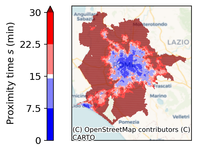
(a)

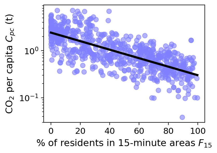
(b)

Figure 1: Impact of the fraction of population residing in 15-minute areas of a city on its transport-related CO₂ emissions. On the left, the division of Rome into ”15-minute” areas, in shades of blue, and ”non-15-minute” areas, in shades of red. Classification is made based on proximity time $s$, which measures the average time a citizen has to walk to access services in a particular area. On the right, a scatter plot of CO₂ emissions per capita versus the fraction of people residing in 15-minute areas $F_{15}$, for different cities worldwide. Cities with a higher fraction of the population with access to local services emit less. The orange line represents an exponential fit ($R^{2}=0.53$).

Road transport is the largest source of CO₂ emissions in the European Union, accounting for around a quarter of total emissions [1], and one observes a similar situation in the US, where 31% of CO₂ emissions is due to transport [2]. In a context in which cities are nowadays held responsible for more than 60% of global greenhouse gases [3], and urban population is rising at the worldwide scale [4], building less car-dependent cities is, therefore, a goal of significant importance in the pathway towards carbon neutrality [5]. Moreover, drastically diminishing the number of vehicles circulating in our cities would address other externalities of car-centred mobility: degradation of air quality [6], deaths and injuries due to road crashes [7], social exclusion, landscape degradation [8], and it would free up public space otherwise necessary to move and park private cars [9].

Since only about $3\%$ of cars worldwide are powered by electricity [10, 11], CO₂ emissions still represent a good marker for studying car usage. Therefore, we will examine CO₂ emissions resulting from transport in cities to quantify car usage and as a target for achieving carbon neutrality.

Various urban planning strategies have been proposed to build less car-centred urban environments. Several studies, in particular, find a significant negative correlation between the population density of cities and their CO₂ emissions for transports [12, 13, 14]; it is argued that this is the case because high population density often matches with mixed land use and pedestrian-oriented urban forms, whereas urban sprawl is associated with longer travel distances and thus with extra fuel and resource consumption [15, 16, 17]. Precisely mixed land use and pedestrian-oriented urban forms are critical ingredients of an urban planning paradigm that has gained growing attention from researchers and policy-makers in recent years: the 15-minute city [18]. In 2016, Carlos Moreno revamped the already-known paradigm of the compact city [19] into this new concept, which aims at constructing cities highly accessible on foot and by bike. In a 15-minute city, every basic need of citizens must be fulfilled within a 15-minute radius of their home, either by foot or bicycle. Such proximity of services aims to enable citizens to walk or cycle to essential amenities, reducing their car dependence. The possibility of a shift towards active mobility is believed to improve environmental sustainability [3, 18, 20, 21], along with health and social cohesion [22]. For this reason, the 15-minute concept has been promoted as part of the post-pandemic Green and Just Recovery Agenda [23] of the C40 Cities, a global network of cities taking action to confront the climate crisis [24]. A case study on Quebec City (Canada) [25] showed that land-use diversity and residential density significantly lower greenhouse gas emissions for transport and motorisation rates, promoting active mobility. Moreover, short journeys are observed in cities with a higher density of Points of Interest (POIs) [26]. Nevertheless, a systematic, large-scale, data-driven evaluation of the impact of implementing the 15-minute concept on car dependency is still lacking.

In this work, we aim to answer whether cities that are more accessible by foot, like 15-minute cities, have lower emissions for transport. Here, we quantify accessibility by foot by the average time citizens should walk from their residence to reach POIs. We take this quantity as a metric for the proximity of services and will refer to it as proximity time, $s$ [22]. We focus on countries labelled as high-income in the World Bank classification [27]. Countries with a lower income have lower motorisation rates [28] and generally worse quality of OpenStreetMap (OSM) data [29], making our analysis less robust. We refer to the Supplementary Information (SI) for further discussion of data regarding lower-income countries.

Here, we find evidence that more accessible cities emit less, showing that cities more adherent to the paradigm of the 15-minute city indeed reduce their emissions. On top of this general trend linking better walking accessibility with lower emissions, we observed substantial fluctuations across cities. We explain these fluctuations in terms of the city size: if two cities with the same foot accessibility spread on different surface areas, on average, the bigger one will emit more. We argue that foot accessibility and the area covered by a city play a pivotal role in determining its CO₂ emissions; hence, we model the effect of these two variables on transport emissions simultaneously. Our results suggest that the proximity of services advocated by the 15-minute city concept, coupled with compact urban planning aiming at smaller urban areas, is effective in fostering sustainable mobility.

Results

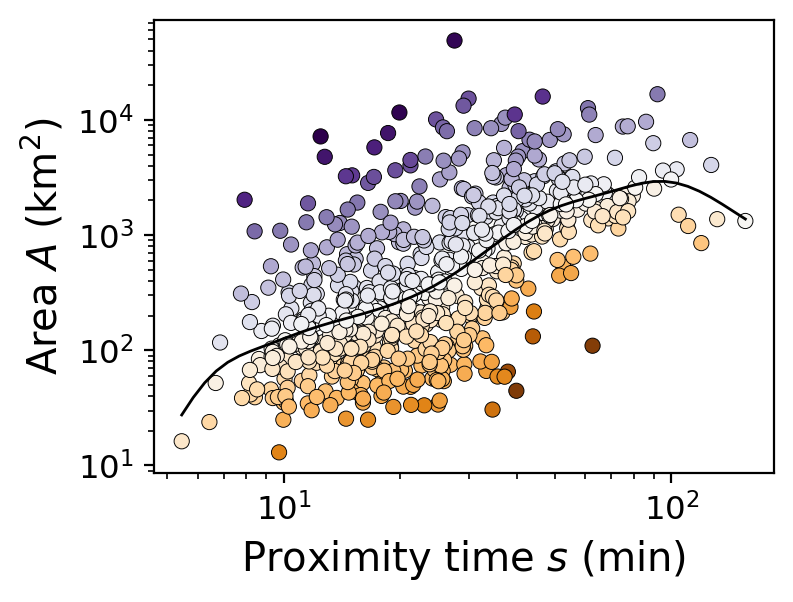
(a)

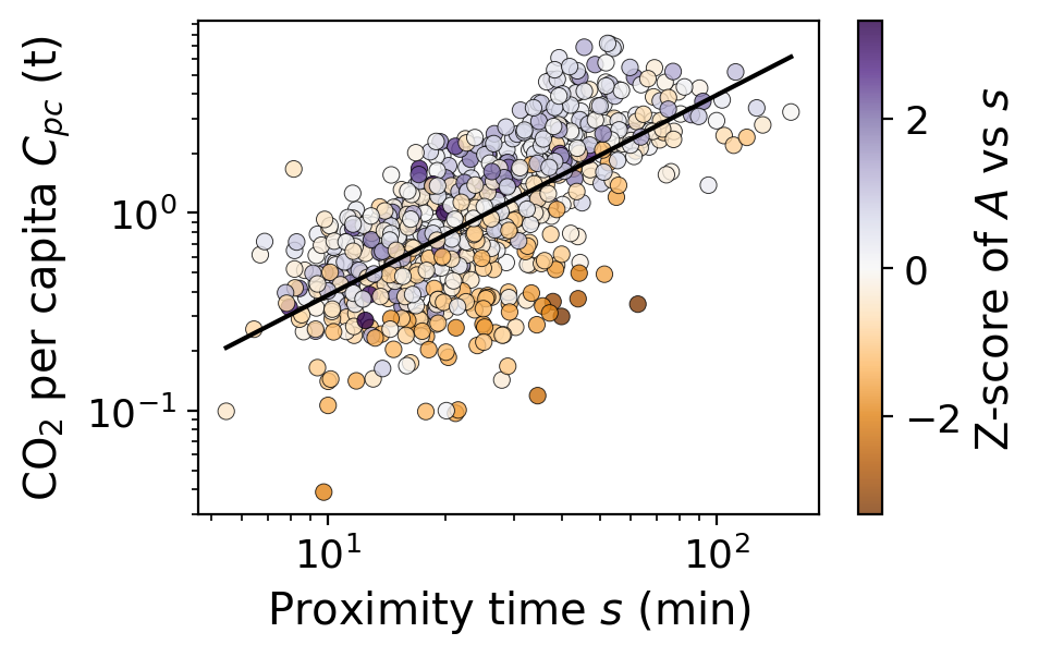
(b)

Figure 2: Accessibility, area and transport CO₂ correlations. On the left, the spatial extension of several cities worldwide is plotted against their proximity time $s$, a measure of walking accessibility, together with a kernel non-parametric regression ($R^{2}=0.42$). Colour encodes the Z-score of the variation of the area of the cities with respect to the average value the kernel non-parametric regression would predict based on their walking accessibility. On the right, the transport-generated CO₂ emitted per capita C${}_{\text{pc}}$ in several cities worldwide versus their proximity time $s$. Data are fitted with a power-law with exponent $\gamma=1.01\pm 0.06$ ($R^{2}=0.47$). Orange points (corresponding to cities covering smaller areas) tend to occupy the region of the right plot under the fitting line; vice versa, purple points (corresponding to cities covering larger areas) tend to populate the region above the fitting line, i.e., emitting more CO₂. In other words, in the plot on the right, the colour gradient correlates with the fluctuations of the data points: Z-scores of the variations of C${}_{\text{pc}}$ and $A$, with respect to their respective fittings, are correlated with a linear correlation coefficient of 0.50. Therefore, on average, more accessible cities emit less; while for the same accessibility, smaller cities emit less than those sprawling in bigger areas.

15-minute cities emissions

To test the effectiveness of more pedestrian-oriented urban forms in fostering sustainable mobility, we analyse 700 cities belonging to high-income countries for which we know the population distribution, the surface extension of the functional urban area, and the CO₂ emissions per capita for transport in the year 2021, the latter based on the EDGAR dataset [30] (see Materials and Methods for a detailed description).

We measure the accessibility for pedestrians of each of these cities with the proximity time $s$, which quantifies how many minutes a citizen has to walk, on average, from their residence to fulfil their everyday needs in the city [31] (we refer to the section Materials and Methods for more details about its computation). The lower the value of this metric is, the fewer minutes one needs to walk to access services, and therefore, the better the walking accessibility of an area. In Fig. (1(a)), the local values of proximity time are shown on a map of Rome.

We can consider an area to be 15-minute if its proximity time $s$ is lower than 15 minutes so that citizens living there have to walk less than a quarter of an hour, on average, to fulfil everyday needs. We quantify, for the cities in our dataset, the fraction of people residing in 15-minute areas, $F_{15}:=P_{15}/P$, where $P_{15}$ indicates the population residing in 15-minute areas, and $P$ the total population of the city [24]. Such fraction correlates with the emissions for transport per capita $C_{\text{pc}}$, as shown in Fig. (1(b)) . One can fit these data with an exponential function of the form:

$$C_{\text{pc}}=C_{0}\,e^{-\frac{F_{15}}{F_{15,0}}}\,,$$ (1)

with the following estimations for the parameters

$$C_{0}=(2.4\pm 0.1)\text{t}\,,\quad F_{15,0}=(48\pm 2)\%\,.$$ (2)

This means that, on average, cities without any 15-minute area, i.e., with $F_{15}=0$, are expected to emit a quantity of CO₂ equal to $C_{0}$ per capita for transport in one year. Since $F_{15,0}\simeq 1/2$, cities having half of their population residing in 15-minute areas lower their emissions of a factor $e\simeq 2.7$ with respect to $C_{0}$. Finally, a switch from an utterly non-15-minute city to an utterly 15-minute one would result, following this simple model, in a reduction of more than a factor seven ($\simeq e^{2}\simeq 7.4$), with respect to $C_{0}$. This finding supports the often-claimed sustainability of the 15-minute city: extending the number of residents living in 15-minute areas, on average, significantly decreases transport carbon emissions.

Interplay between walking accessibility and city surface extension in driving CO₂ production

Proximity time can also characterise the global city’s accessibility by foot: more accessible urban areas have lower average proximity time. In Fig. (2(b)), the CO₂ emissions $C_{\text{pc}}$ per capita of road and rail transports of the urban areas are plotted against their average proximity time $s$. We report a correlation between proximity time and transport emissions, which we can quantify using the linear correlation coefficient between the logarithms of $s$ and $C_{\text{pc}}$, which yields a value of 0.68. We also fit these data with a power law of the form:

$$C_{\text{pc}}\sim s^{\gamma}\,,\quad\gamma=1.01\pm 0.06\,.$$ (3)

Moreover, our research reveals the interplay between these quantities and city areas. The relationship between proximity time and city area is evident in Fig. (2(a)): cities that cover a smaller area have lower proximity times and better walking accessibility. We perform a kernel non-parametric regression of city areas against proximity time to estimate the average trend. This result enables us to calculate the Z-score for each city’s actual area relative to the area predicted by the regression based on its accessibility. In Fig. (2), we colour the points representing cities according to such Z-score in both plots. Cities with a positive Z-score cover larger areas than average for their degree of accessibility by foot; vice versa, cities with a negative Z-score are smaller in area than the average city with the same accessibility level. See SI for details on how Z-scores have been computed. Fig. (2(b)) shows that accessibility and emissions are correlated so that a city with good accessibility will, on average, pollute less than one with bad accessibility. Still, there are many deviations from this average trend. These fluctuations can be explained by the Z-score, encoded by the colour and, therefore, by the different areas covered by the cities. On average, cities that spread over larger areas than average, given their walking accessibility, also feature more significant emissions; vice versa, cities insisting on smaller areas have lower emissions. This trend can be verified by computing the Z-score of CO₂ emissions of cities with respect to the value predicted by the power-law fit (Eq. 3) based on their degree of walking accessibility. The correlation coefficient between the two Z-scores described is 0.50, and in the SI we show their scatter plot. This correlation indicates that a second factor to explain emissions, in addition to the proximity of services in a city, is the total surface covered by the city. In fact, after accounting for their degree of accessibility, large cities pollute more per capita: a low-emissions city needs to be 15-minute but also compact.

It is crucial to note that our findings have direct and significant policy implications. Merely providing services of proximity is insufficient. If cities continue to expand their occupied area, they will also increase their emissions. This evidence underscores the importance of the 15-minute city concept, which should be integrated with regulatory policies that control the size of the city. However, pursuing higher residential density and diversified land use, central to achieving proximity of services, may inadvertently exert upward pressure on housing prices [25].

Unified framework for predicting CO₂ emissions on the basis of walking accessibility and city surface extension

To improve the predictive power of our fitting model (Eq. (3)), we can combine accessibility and city area into a unified framework. Building on the methodology proposed by Ribeiro et al. [14], we can use the Cobb–Douglas production function [32]. It was initially proposed in the context of economics to model the effect of labour and capital on production. Using it here means intending the emission of CO₂ as a production process mediated by cities, which takes accessibility and area as the inputs [14]. In this context, it takes the following form:

$$C_{\text{pc}}\sim s^{\gamma_{s}}A^{\gamma_{A}}\,,$$ (4)

where $C_{\text{pc}}$ represents CO₂ emissions per capita due to transport, $s$ proximity time and $A$ city area. Fitting data with this model, we obtain $R^{2}=0.62$, a value significantly larger than the ones obtained by modelling CO₂ emissions as a function of $s$ or $A$ separately. This finding shows how walking accessibility and the area covered by a city are relevant information for predicting its transport CO₂ emissions. The values of the fitted exponents are

$$\gamma_{s}=0.53\pm 0.05\,,\,\,\gamma_{A}=0.30\pm 0.02\,.$$ (5)

In Fig. (3), we plot the CO₂ emissions $C_{\text{pc}}$ predicted through Eq. (4) for proximity times and city surfaces covering the range of our data. Lower emissions, represented by darker shades of green, are associated with smaller city areas and lower average proximity times. The actual data points, each representing a city, are superimposed on the model’s prediction and encoded in the same colour scheme, giving a visual guide on the agreement between the model and data. We refer to the SI for alternative model schemes.

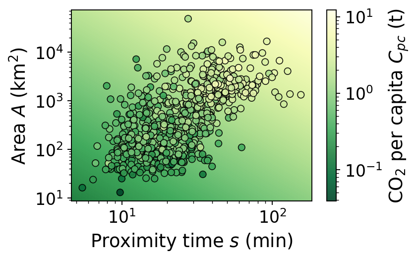
Figure 3: Two-dimensional regression for proximity time, area and CO₂. The points of the scatter plot represent actual data of the cities, while the background gradient is the prediction of our model, Eq. (4) ($R^{2}=0.62$).

Discussion and conclusions

It is often argued that switching from internal combustion engines to electric ones could address one of the main issues related to cars: greenhouse gases and pollutants emissions. Indeed, if we managed to produce energy from carbon-neutral sources within the energy transition framework, switching private cars to electric vehicles would significantly reduce the carbon footprint of transportation [33]. Even with current electricity production methods, the life cycle assessment of electric vehicles shows a decrease in global warming potential compared to internal combustion engine vehicles, even if grid-independent hybrid electric vehicles and high-efficiency internal combustion engine ones outperform electric vehicles powered by coal-fired electricity. However, the production phase of electric vehicles tends to show higher global warming potential than that of internal combustion engine vehicles, primarily due to the impact of battery production [34, 35]. Nevertheless, if a sustainable production of EVs is viable, electric mobility would be a vital component of the green transition [36].

As for air quality, taking action is imperative, too, since the WHO warns that air pollution exceeds recommended levels in 83% of high-income cities and 99% of low-income cities that are monitoring air quality [37], leading to an increasing number of patients with respiratory diseases, cancer, and heart disease globally [3]. Electric vehicles could address this issue since complete turnover to electricity as the vehicle’s power source would lead to a significant reduction of both O₃ and fine particulates (PM_2.5) in cities [38]. But on top of greenhouse gases and pollutants emissions, cars in cities present other drawbacks that would be left untouched even in the scenario of a complete transition towards electricity-powered vehicles: the massive demand for public space that needs to be allocated for parking and moving cars, which can lead to an unfair distribution of urban space [39], the impact of the maintenance of the road infrastructure and, most importantly, the high rate of fatalities due to road accidents. Worldwide, the number of people killed in road traffic accidents each year is estimated to be almost 1.2 million (15 deaths every 100.000 people), while the number of people injured could be as high as 50 million [7], and these rates are always increasing [40]. The most significant burden is in low-income and middle-income countries, with, for example, a mortality rate estimated to be equal to 17.2 deaths per year for every 100.000 people in India [41]. Therefore, switching from internal combustion engines to electric ones would solve some car drawbacks. At the same time, a shift from private vehicles to active mobility and public transport in cities would address the issues mentioned. While fostering decarbonisation, it would increase urban safety and livability [5].

Here, we identified some city features that effectively make such a mode shift possible. Through a large-scale comparison between cities worldwide, we showed that, in high-income countries, cities with greater walking accessibility to essential services significantly reduce CO₂ emissions for transport. Approximately 40 kg of CO₂ is saved per capita annually for each minute reduced on the proximity time $s$. This reduction results from decreased reliance on private cars, a shift facilitated by the lower car dependency of citizens obtained through enhanced walking accessibility. A shining example of such a city is the 15-minute city; our research revealed that cities with a more significant proportion of their population residing in 15-minute areas also exhibit lower transport emissions. Implementing the 15-minute city policy can be a powerful tool in the fight against greenhouse gas emissions and car dependency, offering a promising path towards more sustainable mobility.

A second important outcome of this work is identifying the area covered by cities as a key driver, intertwined with walking accessibility, for urban CO₂ emissions. Since cities spreading over smaller areas have, on average, better walking accessibility, we had to disentangle the two effects. Once we decoupled the effects on CO₂ emissions of walking accessibility and city area, we showed that the fluctuations in CO₂ emissions, on top of the general trend linking better accessibility to lower emissions, are well described by fluctuations in area; cities extending on smaller areas tend to emit less than those sprawling on more extensive surfaces.

The combined influence of walking accessibility and surface area in explaining CO₂ transport emissions of cities has allowed us to develop a model that incorporates these two factors simultaneously, thereby enhancing the predictive power of our study compared to models that consider only one of these factors. This outcome underscores the significance of our findings and their potential to inform and guide future urban planning and policy decisions: the combination of walking accessibility and compactness fosters sustainable mobility in cities.

In summary, our work shows that proximity-based cities, e.g., 15-minute cities, successfully foster more sustainable mobility. City areas also have an additional effect on transport emissions. Therefore, to further meet sustainability goals, the proximity of services has to be combined with efficient public transport and urban planning aimed at containing urban sprawl.

Materials and Methods

Data

EDGAR

The EDGAR dataset [30, 42], from the European Union, contains a gridded estimation of air pollutant emissions worldwide, divided by sectors, from 1970 until 2021. Emissions are expressed in the mass of pollutants emitted per unit of time and area. Estimations are based on fuel combustion data.

The emissions per country and compound are calculated annually and sector-wise by multiplying the country-specific activity and technology mix data by country-specific emission factors and reduction factors for installed abatement systems for each sector. Regarding fossil CO₂ emissions, all anthropogenic activities leading to climate-relevant emissions are considered in the country activity, except biomass/biofuel combustion (short-cycle carbon). Land use, land-use change and forestry (LULUCF) are also sources for EDGAR estimations for CO₂ emissions. EDGAR dataset builds up on the IEA CO₂ emissions from fossil fuel combustion [43] providing estimates from 1970 to 2019 by country and sector, based on data on fuel combustion. These emissions are then extended with a Fast Track approach until 2021 using the British Petroleum statistics for 2020 and 2021 [42].

In this work, we focused on the CO₂ emitted due to transport (particularly by road vehicles and rail transportation) in 2021.

15-minute city platform

The 15-minute platform developed by Sony CSL Rome [31] quantifies for several cities worldwide the average minutes one citizen needs to walk or ride a bike before getting to one of the 20 closest Points of Interest (POIs) where they can fulfil one of the following needs: learning, healthcare, eating, supplies, moving (with public transport), cultural activities, physical exercise, and other services. This average time $s$ quantifies the degree of proximity of services from residential areas in a given city; for this reason, we referred to it as “proximity time”. In the original formulation of the 15-minute city [18], this time should be no more than 15 minutes for every citizen, for every need. The platform then allows one to explore the degree of proximity of services in different areas of the cities analysed by showing the metric $s$ on a hexagonal grid composed of elements of lateral size $200$ m.

Methodology

Z-scores calculation

The kernel non-parametric regression, used to estimate the average surface extension of cities with a given proximity time, has been computed using a local linear estimator and a Gaussian kernel of bandwidth set using the AIC Hurvich bandwidth estimation in logspace. Thanks to such regression, it has been possible to calculate the Z-scores of a city’s area relative to the average value for its degree of accessibility, the latter measured by proximity time. To do so, we proceeded as follows: we divided the cities into four quartiles based on their mean proximity time. The quartiles are visible in SI. For each city $j$, belonging to each quartile $i$, we calculated the residual $\delta_{j}$ between the logarithm of its actual area $A_{j}$ and the logarithm of the average area for its proximity time estimated by the kernel regression $\bar{A}(s_{j})$:

$$\delta_{j}=\text{log}_{10}(A_{j})-\text{log}_{10}(\bar{A}(s_{j}))\,.$$

The distributions of the residuals $\delta_{j}$ inside each quartile $i$ are all compatible at $3\sigma$ C.L. with normality. The two-sided p values, for each quartile, of the K.S. test for the null hypothesis that the residuals $\delta_{j}$ are normally distributed are p${}_{1}=0.02$, p${}_{2}=0.02$, p${}_{3}=0.7$, p${}_{4}=0.3$. We therefore computed the standard deviation of the residuals, obtaining four standard deviations $\sigma_{i}$, $i=1,...,4$. The Z-score of the area of a city $j$ belonging to quartile $i$ is therefore given by:

$$Z_{j}=\frac{\delta_{j}}{{\sigma_{i}}}\,.$$ (6)

Z-scores of variations of CO₂ emissions per capita with respect to the prediction of the power-law model of Eq. (3) would predict based on the city’s proximity time has been computed following the same procedure. Residuals this time do not differ from Gaussianity at 95 % C.L., being the K.S. two-sided p values of the four quantiles p${}_{1}=0.4$, p${}_{2}=0.9$, p${}_{3}=0.3$ and p${}_{4}=0.2$.

Fitting procedures

The exponential fit of Eq. (1) has been performed as a linear least squares regression between the fraction of residents in 15-minute areas $F_{15}$ and the logarithm of emissions $C_{\text{pc}}$. The confidence intervals on two parameters $C_{0}$ and $F_{15,0}$ have been estimated via bootstrapping [44]. Running the algorithm for $40\,000$ iterations gave the same number of estimations of log$A$ and $1/F_{15,0}$. We deduced an estimation of $A$ and $F_{15,0}$ from each of those estimations. The results are collected in the histograms in SI. The resulting probability density distributions are not Gaussian at 95% C.L. (K.S. test). Confidence intervals for the fitted parameters have been estimated as symmetric intervals around the mean value enclosing 68$\%$ of the probability. The power-law fits of Eqs. (3) and (4) have been performed using a least-squares linear regression between logarithms of the quantities involved. All $R^{2}$ scores have to be intended as referred to these fits in the log space. The confidence interval for the exponent $\gamma$ of the fitting in Eq. (3) has been computed using least-squares minimization considering equal measuring errors on $C_{\text{pc}}$ and $s$; considering errors on log$(s)$ linearly propagating on log$(C_{\text{pc}})$, the error $\sigma_{\gamma}$ on the parameter $\gamma$ was estimated as

$$\sigma_{\gamma}^{2}=\left(1+\gamma^{2}\right)\tilde{\sigma}_{\gamma}^{2}\,,$$

where $\tilde{\sigma}_{\gamma}$ represents the error the least-squares minimization would prescribe for the parameter in the standard case in which only the quantity on $y$, log$(C_{\text{pc}})$, is affected by measuring errors [45].

Average city proximity time estimation

The average proximity time $s$ for a city has been calculated using a weighted mean approach. This approach consists of averaging the proximity time values ($s$) across all hexagonal cells within the grid defined in [31], with population serving as the weighting factor for each cell.

Correlations

Linear correlation coefficients are estimated using the Pearson correlation coefficient.

Competing interests

The authors declare no competing interests.

Materials and Correspondence

Supplementary information

This work contains supplementary material.

Correspondence

Correspondence and material requests should be addressed to Francesco Marzolla (francesco.marzolla@uniroma1.it).

2

Supplementary Information

Appendix A Lower-income countries

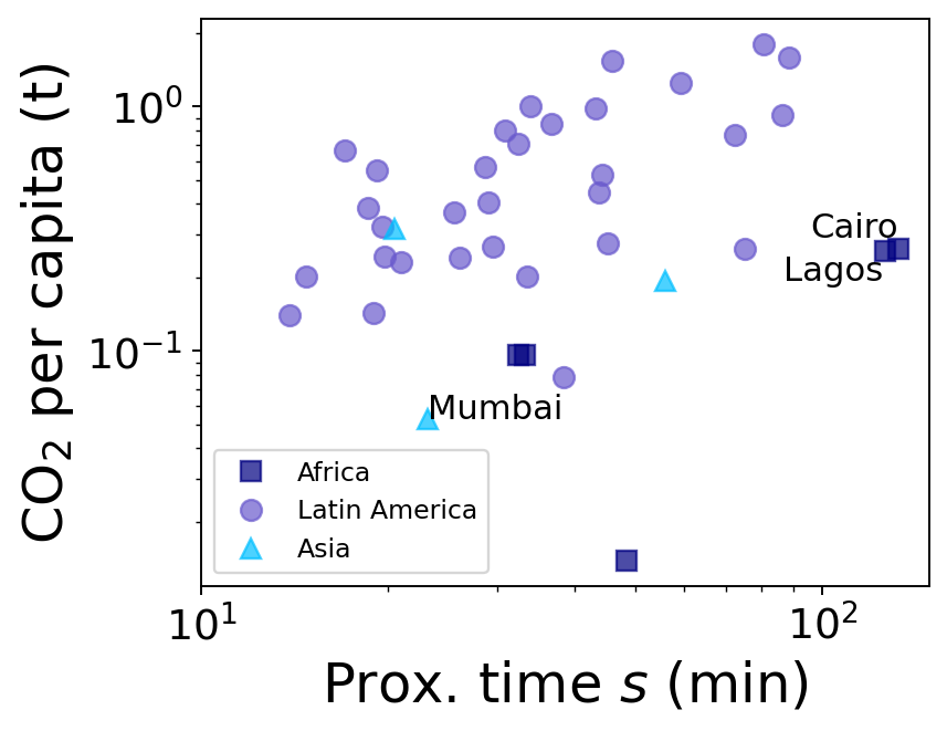
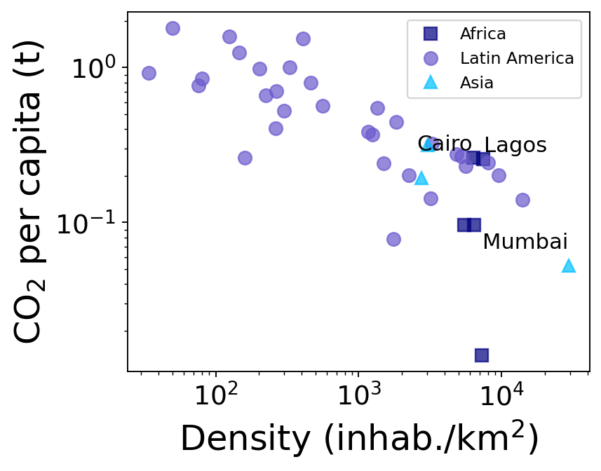
Figure 4: CO₂ emissions for transports (road and rail transport) per capita in 2021, in tonnes, versus the average proximity time, in mins, to POIs for city residents in lower-income countries. Each dot represents an urban area, and its dimensions are proportional to the resident population. Different colours and shapes encode different macroregions.

For cities of high-income countries [27], the logarithm of the proximity time $s$ has a linear correlation coefficient of 0.68 $R^{2}=0.68$ with the logarithm of the CO₂ for transports per capita. In contrast, cities in lower-income countries display a correlation coefficient of just 0.25.

We hypothesize two factors as possible drivers of the vanishing correlation in the Global South: the lower coverage and reliability of the data used to compute the proximity time $s$ and the higher difficulty for people residing in those areas to own a car.

Regarding the first issue, the destinations of the trips to access everyday services, whose average length constitutes our proximity time $s$, are Points of Interest taken from OpenStreetMap (OSM). OSM is an open platform where private contributors can map the geography of places where they reside, have travelled or even have studied remotely with satellite images. As demonstrated in [46], there is an observed decline in the quality of POIs coverage on OSM in regions with lower socioeconomic status. In particular, Lagos, in Nigeria, is one of the cities that deviate the most from the general approximate power-law relation between proximity and emissions, which holds in high-income countries. In [47], it was shown the existence in 2021 of a slum in Lagos completely not mapped in OSM. The existence of this kind of urban area in developing countries makes it even more challenging to map cities accurately because of the tendency of these areas to be destroyed and rebuilt more rapidly than other types of settlements. To highlight possible overestimations of the proximity time $s$, we can exploit the fact that in the very first approximation, the degree of pedestrian accessibility of services of a city can be estimated by its population density. This is a brute approximation since it does not consider the details of the city’s design, whose relation with CO₂ emissions is precisely the target of this study. Still, it can give insight into which cities have an estimated accessibility very different from the one expected by their density. Cities that present carbon emissions out of range with respect to their proximity time $s$, such as Mumbai, Cairo and Lagos, align to the general trend if one considers emissions as a function of their density instead. This evidence could be a sign of overestimation of the proximity time for these cities due to a lack of OSM data.

From the side of the different access to cars by people residing in cities located in different areas of the World, in the year 2019 the average vehicle ownership in the EU (motorization rate) was 57 cars per 100 inhabitants [48], in 2021 in the United States it was equal to 84 cars per 100 inhabitants [49], while in 2019 in India it was equal to 23 cars per 100 inhabitants [50] and in 2018 in Nigeria to only six cars per 100 inhabitants [51]. These data can be read as part of a general trend, studied and modelled in [28], which links higher GDP per capita to higher vehicles/population ratio for different countries.

Figure 4b shows the relation between CO₂ emissions for transports per capita in 2021 and population density for the cities of lower-income countries.

Because of this looser bond between proximity time and emissions for lower-income countries, we decided to restrict our study to cities in high-income countries, where the dynamics at play are more akin. Fig. 5 shows how the geographical subdivision, among high-income countries, of the cities studied influences their position in the CO₂ emissions vs proximity time plane. In particular, cities in the USA and Canada tend to emit more for transport and have worse proximity times with cities in other high-income countries.

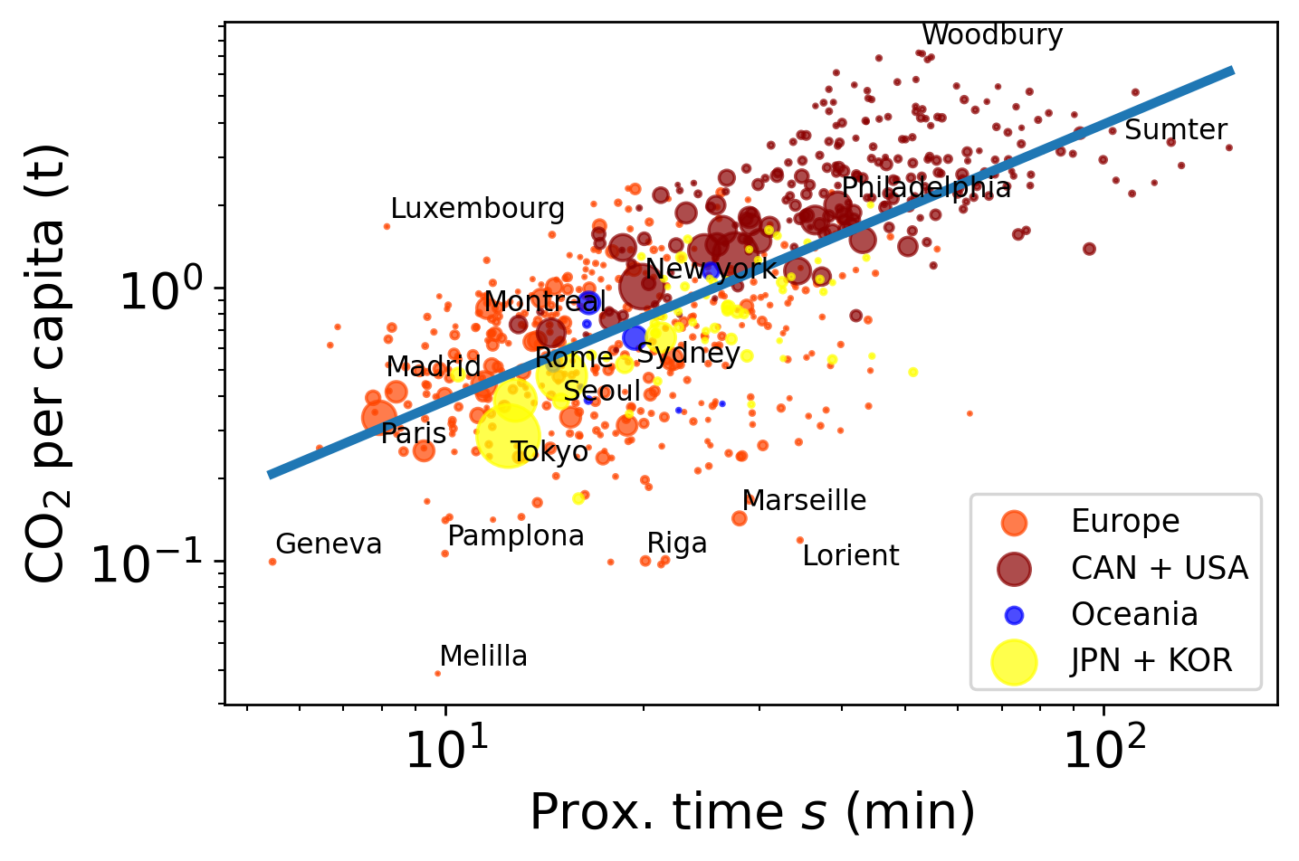
Figure 5: Geographical subdivision of the studied cities. CO₂ emissions for transports (road and rail transport) per capita in 2021, in tonnes, versus the average proximity time, in mins, of the cities studied. Each dot represents an urban area, and its dimensions are proportional to the resident population. All cities belong to high-income countries, and the macro-region in which they are located is encoded by colour in the plot. CAN stands for Canada, JPN for Japan and KOR for South Corea. The line overimposed on data is the graph of a fitted power law of the form $C_{pc}\sim s^{\gamma}$, with $\gamma=1.01\pm 0.04$.

Appendix B Correlation between fluctuations on area and on emissions

Fig. (6) depicts, for the cities under study, the relation between fluctuations on area and on emissions respect to the expected values based on the walking accessibility of cities. Fluctuations in emissions are positively correlated with fluctuations in area, with linear correlation coefficient $r=0.50$. This means that cities covering a larger area than the average for their degree of walking accessibility, tend to emit more for transport, than expected from their degree of walking accessibility.

Fluctuations are quantified via Z-scores in logspacewith the following procedure. The Z-score of a city $j$ with area $A_{j}$ and proximity time $s_{j}$, belonging to the quartile $i$ of the proximity time distribution, is given by:

$$Z_{j}=\frac{{A_{j}-\bar{A}(s_{j})}}{{\sigma_{i}}}\,,$$ (7)

where $\bar{A}(s)$ is the average value of area for proximity time $s$, estimated by the kernel regression. The $p$-value at which it is possible to reject the null hypothesis that the residuals at the numerator of Eq. (7) are normally distributed is 0.006 (K.S. test). Being not possible to reject the null hypothesis of normality at $3\sigma$ C.L., we went on computing the standard deviation of residuals in each quartile, $\sigma_{i}$, and finally computed $Z_{j}$ for each city. Quartiles are depicted in different colors in Fig. (7(a)). The same procedure has been used to compute Z-scores of actual CO₂ emissions of cities respect to the ones predicted on the basis of their average proximity time. Quartiles and the power-law model used to predict expected emissions are visible in figure (7(b)).

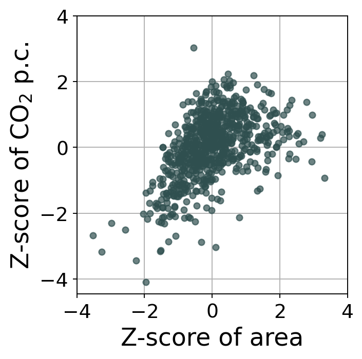
Figure 6: Fluctuations on city areas are correlated with fluctuations on emissions for transport, with linear correlation coefficient $r=0.50$. Each dot represents a city worldwide. On the two axes are depicted respectively the Z-scores of emissions and area respect to some estimation of the expected values of these quantities based on the walking accessibility of the city considered. The expected values are estimated for emissions via a power-law regression of emissions versus proximity time, and for area as a kernel non-parametric regression of area versus proximity time.

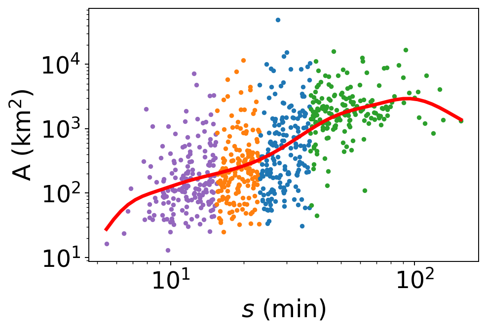
(a)

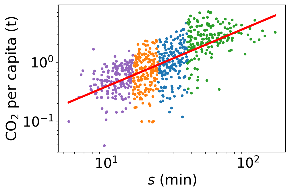
(b)

Figure 7: Quartiles, encoded by colour, and fitted models used to estimate Z-scores of city areas (a), and of CO₂ emissions (b).

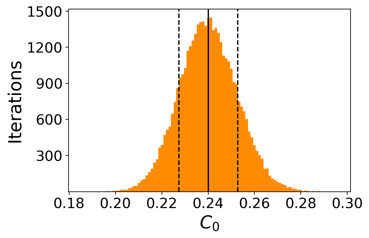
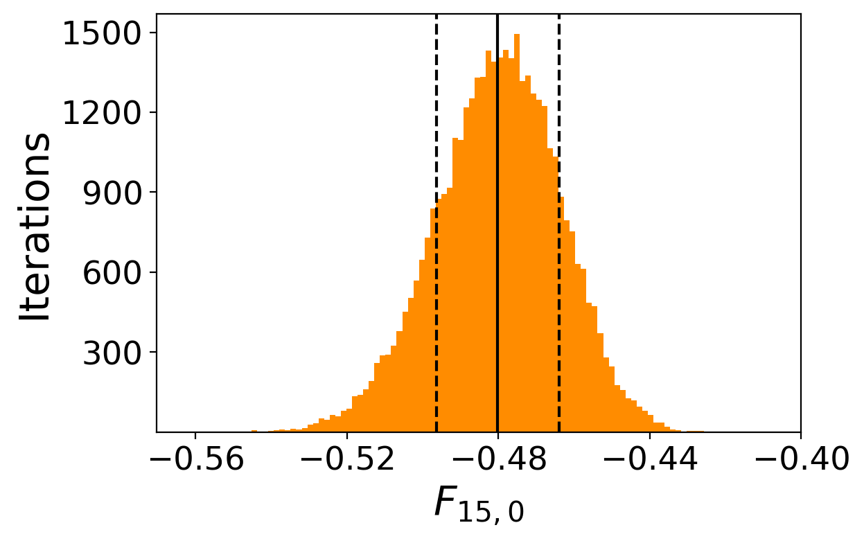
Figure 8: Probability density functions of the parameters of the exponential fit of $C_{\text{pc}}$ vs $F_{15}$. The solid line marks the mean value of each distribution, while the dashed lines delimit the confidence interval, corresponding to $68\%$ of the probability. The histograms collect the parameters obtained running for $40\,000$ iterations of a bootstrapping algorithm.

Appendix C Confidence intervals on the fitted parameters

The confidence intervals of the parameters of the exponential fit of $C_{\text{pc}}$ vs $F_{15}$ have been estimated by bootstrapping. Running the algorithm for $40\,000$ iterations gave the same number of estimations of log$A$ and $1/F_{15,0}$. From each of those estimations, we deduced an estimation of $A$ and $F_{15,0}$. The results are collected in the histograms in Fig. (8). The resulting probability density distributions are not Gaussian at 95% C.L.. Confidence intervals for the fitted parameters have been therefore estimated as symmetric intervals around the mean value enclosing 68$\%$ of the probability.

Appendix D Alternative modelling of CO₂ emissions

With the same number of parameters as the Cobb-Douglas function used in the main text, we could also model the relationship between emissions, proximity time and city area in the following way, therefore adding an interaction term between proximity time and city area:

$$\text{log}(C_{pc})=\zeta\,\text{log}(s)+\xi\,\text{log}(A)+\phi\,\text{log}(s)\,\text{log}(A)+\nu\,,$$ (8)

which yields $R^{2}=0.63$, therefore an accuracy compatible with the Cobb-Douglas model, which does not include the interaction term. The values of the parameters resulting from a least-squares fit are:

$$\zeta=-1.8\pm 0.6\,,\quad\xi=-0.1\pm 0.1\,,\quad\phi=0.26\pm 0.07\,,\quad\nu=-0.2\pm 0.9\,.$$ (9)

All confidence intervals have been estimated via bootstrapping.

Appendix E Cities’ metrics

All cities studied are collected, with their key metrics, in table E.

[ longtable= l—ccccc, table head=Cities’ metrics: population, area, proximity time, and annual CO₂ emissions for transport per capita
City Country Population A (km²) $s$ (min) C${}_{\text{pc}}$ (t)
, late after line=
, late after last line=
, column count=6 ]Supplementary_Information/citt_per_SI.csv

References

- [1] EEA “Annual European Union greenhouse gas inventory 1990–2019 and inventory report 2021”
- [2] Anthony Underwood and Anders Fremstad “Does Sharing Backfire? A Decomposition of Household and Urban Economies in CO2 Emissions” In Energy Policy 123, 2018, pp. 404–413 DOI: 10.1016/j.enpol.2018.09.012
- [3] Zaheer Allam, Mark Nieuwenhuijsen, Didier Chabaud and Carlos Moreno “The 15-minute city offers a new framework for sustainability, liveability, and health” In The Lancet Planetary Health 6.3 Elsevier, 2022, pp. e181–e183
- [4] United Nations “World Urbanization Prospects The 2018 Revision”
- [5] International Transport Forum “ITF Transport Outlook 2023”, ITF Transport Outlook OECD, 2023 DOI: 10.1787/b6cc9ad5-en
- [6] Timothy J Wallington, James E Anderson, Rachael H Dolan and Sandra L Winkler “Vehicle emissions and urban air quality: 60 years of progress” In Atmosphere 13.5 MDPI, 2022, pp. 650
- [7] Margie M Peden “World report on road traffic injury prevention” World Health Organization, 2004
- [8] Marco Te Brömmelstroet et al. “Identifying, nurturing and empowering alternative mobility narratives” In Journal of urban mobility 2 Elsevier, 2022, pp. 100031
- [9] Thalia Verkade and Marco Te Brömmelstroet “Movement: how to take back our streets and transform our lives” Island Press, 2024
- [10] IEA “Cars and vans” URL: https://www.iea.org/energy-system/transport/cars-and-vans
- [11] “Global EV Outlook 2024”, 2024 URL: https://www.iea.org/reports/global-ev-outlook-2024
- [12] Ramana Gudipudi et al. “City density and CO2 efficiency” In Energy Policy 91 Elsevier, 2016, pp. 352–361
- [13] Albert Hans Baur, Maximilian Thess, Birgit Kleinschmit and Felix Creutzig “Urban climate change mitigation in Europe: looking at and beyond the role of population density” In Journal of Urban Planning and Development 140.1 American Society of Civil Engineers, 2014, pp. 04013003
- [14] Haroldo V Ribeiro, Diego Rybski and Jürgen P Kropp “Effects of changing population or density on urban carbon dioxide emissions” In Nature communications 10.1 Nature Publishing Group UK London, 2019, pp. 3204
- [15] Hong Ye et al. “A sustainable urban form: The challenges of compactness from the viewpoint of energy consumption and carbon emission” In Energy and Buildings 93 Elsevier, 2015, pp. 90–98
- [16] Elizabeth Burton “The compact city: just or just compact? A preliminary analysis” In Urban studies 37.11 Sage Publications Sage UK: London, England, 2000, pp. 1969–2006
- [17] Ago Yeh and Xia Li “The need for compact development in the fast growing areas of China: The Pearl River Delta” In Compact cities: Sustainable urban forms for developing countries E & FN Spon, 2000, pp. 73–90
- [18] Carlos Moreno et al. “Introducing the “15-Minute City”: Sustainability, resilience and place identity in future post-pandemic cities” In Smart Cities 4.1 MDPI, 2021, pp. 93–111
- [19] Christine Haaland and Cecil Konijnendijk Den Bosch “Challenges and strategies for urban green-space planning in cities undergoing densification: A review” In Urban forestry & urban greening 14.4 Elsevier, 2015, pp. 760–771
- [20] Amir Reza Khavarian-Garmsir, Ayyoob Sharifi and Ali Sadeghi “The 15-minute city: Urban planning and design efforts toward creating sustainable neighborhoods” In Cities 132 Elsevier, 2023, pp. 104101
- [21] Zaheer Allam, Simon Elias Bibri, Didier Chabaud and Carlos Moreno “The theoretical, practical, and technological foundations of the 15-minute city model: proximity and its environmental, social and economic benefits for sustainability” In Energies 15.16 MDPI, 2022, pp. 6042
- [22] Matteo Bruno, Hygor Piaget Monteiro Melo, Bruno Campanelli and Vittorio Loreto “A universal framework for inclusive 15-minute cities” In Nature Cities xx.xx, 2024, pp. xxx–xxx URL: http://arxiv.org/abs/2408.03794
- [23] “C40 mayors’ agenda for a green and just recovery.”, 2020
- [24] TM Logan et al. “The x-minute city: Measuring the 10, 15, 20-minute city and an evaluation of its use for sustainable urban design” In Cities 131 Elsevier, 2022, pp. 103924
- [25] François Des Rosiers, Marius Theriault, Gjin Biba and Marie-Hélène Vandersmissen “Greenhouse gas emissions and urban form: Linking households’ socio-economic status with housing and transportation choices” In Environment and Planning B: Urban Analytics and City Science 44.5 SAGE Publications Sage UK: London, England, 2017, pp. 964–985
- [26] Anastasios Noulas et al. “A Tale of Many Cities: Universal Patterns in Human Urban Mobility” In PLoS ONE 7.5, 2012, pp. e37027 DOI: 10.1371/journal.pone.0037027
- [27] URL: https://datahelpdesk.worldbank.org/knowledgebase/articles/906519-world-bank-country-and-lending-groups
- [28] Joyce Dargay and Dermot Gately “Income’s effect on car and vehicle ownership, worldwide: 1960–2015” In Transportation Research Part A: Policy and Practice 33.2, 1999, pp. 101–138 DOI: https://doi.org/10.1016/S0965-8564(98)00026-3
- [29] Benjamin Herfort et al. “A spatio-temporal analysis investigating completeness and inequalities of global urban building data in OpenStreetMap” In Nature Communications 14.1 Nature Publishing Group UK London, 2023, pp. 3985
- [30] JRC European Commission “EDGAR (Emissions Database for Global Atmospheric Research) Community GHG Database (a collaboration between the European Commission, Joint Research Centre (JRC), the International Energy Agency (IEA), and comprising IEA-EDGAR CO2, EDGAR CH4, EDGAR N2O, EDGAR F-GASES version 7.0”, 2022 URL: https://edgar.jrc.ec.europa.eu/dataset_ghg70
- [31] URL: http://whatif.sonycsl.it/15mincity/
- [32] Charles W Cobb and Paul H Douglas “A theory of production” American Economic Association, 1928
- [33] Eckard Helmers and Patrick Marx “Electric Cars: Technical Characteristics and Environmental Impacts” In Environmental Sciences Europe 24.1, 2012, pp. 14 DOI: 10.1186/2190-4715-24-14
- [34] Troy R. Hawkins, Ola Moa Gausen and Anders Hammer Strømman “Environmental Impacts of Hybrid and Electric Vehicles—a Review” In The International Journal of Life Cycle Assessment 17.8, 2012, pp. 997–1014 DOI: 10.1007/s11367-012-0440-9
- [35] Rickard Arvidsson, Mudit Chordia and Anders Nordelöf “Quantifying the Life-Cycle Health Impacts of a Cobalt-Containing Lithium-Ion Battery” In The International Journal of Life Cycle Assessment 27.8, 2022, pp. 1106–1118 DOI: 10.1007/s11367-022-02084-3
- [36] ITF “Transport Outlook 2023” OECD Publishing, Paris. DOI: 10.1787/b6cc9ad5-en
- [37] World Health Organization “Improving the capacity of countries to report on air quality in cities: users’ guide to the repository of United Nations tools” In Improving the capacity of countries to report on air quality in cities: users’ guide to the repository of United Nations tools, 2023
- [38] Shuai Pan et al. “Potential Impacts of Electric Vehicles on Air Quality and Health Endpoints in the Greater Houston Area in 2040” In Atmospheric Environment 207, 2019, pp. 38–51 DOI: 10.1016/j.atmosenv.2019.03.022
- [39] Luis A Guzman, Daniel Oviedo, Julian Arellana and Victor Cantillo-García “Buying a car and the street: Transport justice and urban space distribution” In Transportation Research Part D: Transport and Environment 95 Elsevier, 2021, pp. 102860
- [40] V. Eksler, S. Lassarre and I. Thomas “Regional Analysis of Road Mortality in Europe” In Public Health 122.9, 2008, pp. 826–837 DOI: 10.1016/j.puhe.2007.10.003
- [41] Rakhi Dandona et al. “Mortality Due to Road Injuries in the States of India: The Global Burden of Disease Study 1990–2017” In The Lancet Public Health 5.2 Elsevier, 2020, pp. e86–e98 DOI: 10.1016/S2468-2667(19)30246-4
- [42] Crippa Monica et al. “CO2 emissions of all world countries” EC: European Commission, 2022 DOI: 10.2760/730164
- [43] “Greenhouse Gas Emissions from Energy - 2021 Edition”
- [44] Jonathan Nevitt and Gregory R Hancock “Performance of bootstrapping approaches to model test statistics and parameter standard error estimation in structural equation modeling” In Structural equation modeling 8.3 Taylor & Francis, 2001, pp. 353–377
- [45] Maurizio Loreti “Teoria degli errori e fondamenti di statistica” In Decibel, Zanichelli, 2006
- [46] Sylwia Borkowska and Krzysztof Pokonieczny “Analysis of OpenStreetMap Data Quality for Selected Counties in Poland in Terms of Sustainable Development” In Sustainability 14, 2022, pp. 3728 DOI: 10.3390/su14073728
- [47] Godwin Yeboah, Joao De Albuquerque, Vangelis Pitidis and Syed Ahmed “Analysis of OpenStreetMap Data Quality at Different Stages of a Participatory Mapping Process: Evidence from Slums in Africa and Asia” In International Journal of Geo-Information 10, 2021 DOI: 10.3390/ijgi10040265
- [48] Georgios Spyropoulos, Panagiotis Nastos, Kostas Moustris and Konstantinos Chalvatzis “Transportation and Air Quality Perspectives and Projections in a Mediterranean Country, the Case of Greece” In Land 11, 2022, pp. 152 DOI: 10.3390/land11020152
- [49] Michelle Megna Ashlee Tilford “Car Ownership Statistics 2023” In Forbes Advisor, 7 March 2023
- [50] URL: https://www.statista.com/statistics/665071/number-of-registered-motor-vehicles-india-by-population/
- [51] National Bureau Statistics of Nigeria “Road Transport Data (Q4 2018)”
2