FC-KAN: Function Combinations in Kolmogorov-Arnold Networks

Abstract

In this paper, we introduce FC-KAN, a Kolmogorov-Arnold Network (KAN) that leverages combinations of popular mathematical functions such as B-splines, wavelets, and radial basis functions on low-dimensional data through element-wise operations. We explore several methods for combining the outputs of these functions, including sum, element-wise product, the addition of sum and element-wise product, quadratic function representation, and concatenation. In our experiments, we compare FC-KAN with multi-layer perceptron network (MLP) and other existing KANs, such as BSRBF-KAN, EfficientKAN, FastKAN, and FasterKAN, on the MNIST and Fashion-MNIST datasets. A variant of FC-KAN, which uses a combination of outputs from B-splines and Difference of Gaussians (DoG) in the form of a quadratic function, outperformed all other models on the average of 5 independent training runs. We expect that FC-KAN can leverage function combinations to design future KANs. Our repository is publicly available at: https://github.com/hoangthangta/FC_KAN.

Keywords Kolmogorov Arnold Networks  $\cdot$ function combinations  $\cdot$ B-splines  $\cdot$ wavelets  $\cdot$ radial basis functions

1 Introduction

Recent work by Liu et al. [1, 2] highlights the use of learnable activation functions as "edges" to fit training data better, in contrast to the traditional use of fixed activation functions as "nodes" in multi-layer perceptrons (MLPs). The foundation of KANs is based on the Kolmogorov-Arnold representation theorem (KART), which asserts that any continuous function of multiple variables can be represented as a sum of continuous functions of a single variable [3]. Motivated by this idea, numerous researchers have worked on creating different types of KANs utilizing widely known polynomials and basis functions. While most of these works use a single function in constructing KANs [4, 5, 6, 7], there are a few works using function combinations in KANs’ structure. Ta [8] designed BSRBF-KAN, by combining B-splines and Gaussian Radial Basis Functions within each network layer using data additions. However, this network encounters a memory issue when performing element-wise operations in high-dimensional data, restricting the use of other element-wise operations, such as element-wise product (Hadamard product). In another work, Yang et al. [9] leveraged function combinations to develop optimal activation functions at each node through an adaptive strategy, overcoming the limitations of single activation functions in their S-KAN and S-ConvKAN models.

In this paper, we propose a novel KAN, FC-KAN (Function Combinations in Kolmogorov-Arnold Networks), which leverages various functions to capture data features throughout the network layers and combines them in low-dimensional spaces, such as the output layer, using various methods mainly based on element-wise operations, including sum, product, the combination of sum and product, quadratic function representation, and concatenation. We avoid using a 3rd-degree function due to its higher computational demands on data tensors, which can lead to memory errors. As a result, the model is able to capture more data features, leading to improved performance on the MNIST and Fashion-MNIST datasets compared to other KAN networks. Additionally, employing n-degree functions aligns with the core concept of KAN, where they are used both to capture input data and to represent data features in the output. We expect this exciting development may lead to the proliferation of basis function combinations in neural networks.

Aside from this section, the paper is organized as follows: Section 2 discusses related work on KART and KANs. Section 3 details our methodology, covering KART, the design of the KAN architecture, several existing KANs, and FC-KAN. Section 4 presents our experiments, comparing FC-KAN variants with MLP and other KANs using data from the MNIST and Fashion-MNIST datasets. Additionally, this section includes a comparison of combination types within FC-KAN. We address some limitations of our study in Section 5. Lastly, Section 6 offers our conclusions and potential directions for future research.

2 Related Works

In 1957, Kolmogorov provided a proof to Hilbert’s 13th problem by showing that any multivariate continuous function can be expressed as a combination of single-variable functions and additions, a concept known as KART [3, 10]. This theorem has been utilized in many studies to develop neural networks [11, 12, 13, 14, 15, 16]. However, there is an ongoing debate about the applicability of KART in neural network design. Girosi and Poggio [17] argued that KART’s relevance to neural networks is questionable because the inner function $\phi_{q,p}$ in Equation 1 may be highly non-smooth [18], which could hinder $f$ from being smooth—a key attribute for generalization and noise resistance in neural networks. Conversely, Kůrková [19] contended that KART is applicable to neural networks, showing that linear combinations of affine functions can effectively approximate all single-variable functions using certain sigmoidal functions.

Despite the long history of KART’s application in neural networks, it had not garnered significant attention in the research community until the recent study by Liu et al. [1]. They suggested moving away from strict adherence to KART and instead generalizing it to develop KANs with additional neurons and layers. Our intuition aligns with this perspective as it helps to mitigate the issue of non-smooth functions when applying KART to neural networks. Consequently, KANs have the potential to outperform MLPs in both accuracy and interpretability for small-scale AI + Science tasks. However, the resurgence of KANs has also faced criticism from Dhiman [20], who argue that KANs are essentially MLPs with spline-based activation functions, in contrast to traditional MLPs with fixed activation functions.

KANs have introduced a new perspective to the scientific community since May 2024. Many KAN designs utilize well-known mathematical functions, particularly those capable of handling curves, such as B-Splines [21] (Original KAN [1], EfficientKAN, BSRBF-KAN [8]), Gaussian Radial Basis Functions (GRBFs) (FastKAN [4], DeepOKAN [22], BSRBF-KAN [8]), Reflection SWitch Activation Function (RSWAF) in FasterKAN [5], Chebyshev polynomials (TorchKAN [23], Chebyshev KAN [7]), Legendre polynomials (TorchKAN [23]), Fourier transform (FourierKAN, FourierKAN-GCF [24]), wavelets [6, 25], and other polynomial functions [26]. While these works focus on single functions to design KANs, Ta [8] mentioned the combination of functions – B-Splines and radial basis functions – in designing KANs. Their BSRBF-KAN showed better convergence on the training data for MNIST and Fashion-MNIST. In another work, Yang et al. [9] utilized function combinations to create optimal activation functions at each node using an adaptive strategy, addressing the drawbacks of single activation functions in their S-KAN model. They also extended S-KAN to S-ConvKAN, which showed superior performance in image classification tasks, outperforming CNNs and KANs with comparable structures.

3 Methodology

3.1 Kolmogorov-Arnold Representation Theorem

A KAN is based on KART, which asserts that any continuous multivariate function $f$ defined on a bounded domain can be represented as a finite combination of continuous single-variable functions and their additions [27, 28]. For a set of variables $\mathbf{x}={x_{1},x_{2},\ldots,x_{n}}$, where $n$ is the number of variables, the multivariate continuous function $f(\mathbf{x})$ is expressed as:

$$f(\mathbf{x})=f(x_{1},\ldots,x_{n})=\sum_{q=1}^{2n+1}\Phi_{q}\left(\sum_{p=1}^{n}\phi_{q,p}(x_{p})\right)$$ (1)

which has two types of summations: the outer sum and the inner sum. The outer sum, $\sum_{q=1}^{2n+1}$, aggregates $2n+1$ terms of $\Phi_{q}$ ($\mathbb{R}\to\mathbb{R}$). The inner sum, on the other hand, aggregates $n$ terms for each $q$, where each term $\phi_{q,p}$ ($\phi_{q,p}\colon[0,1]\to\mathbb{R}$) denotes a continuous function of a single variable $x_{p}$.

3.2 The design of KANs

Remind an MLP that consists of affine transformations and non-linear functions. Starting with an input $\mathbf{x}$, the network processes it through a series of weight matrices across layers (from layer $0$ to layer $L-1$) and applies the non-linear activation function $\sigma$ to produce the final output.

$$\text{MLP}(\mathbf{x}) =(W_{L-1}\circ\sigma\circ W_{L-2}\circ\sigma\circ\cdots\circ W_{1}\circ\sigma\circ W_{0})\mathbf{x}$$ (2)

$$=\sigma\left(W_{L-1}\sigma\left(W_{L-2}\sigma\left(\cdots\sigma\left(W_{1}\sigma\left(W_{0}\mathbf{x}\right)\right)\right)\right)\right)$$

Inspired by KART, Liu et al. [1] developed KANs but recommended extending the approach to incorporate greater network widths and depths. To address this, appropriate functions $\Phi_{q}$ and $\phi_{q,p}$ need to be identified. A typical KAN network with $L$ layers processes the input $\mathbf{x}$ to produce the output as follows:

$$\text{KAN}(\mathbf{x})=(\Phi_{L-1}\circ\Phi_{L-2}\circ\cdots\circ\Phi_{1}\circ\Phi_{0})\mathbf{x}$$ (3)

which $\Phi_{l}$ is the function matrix of the $l^{th}$ KAN layer or a set of pre-activations. Let denote the neuron $i^{th}$ of the layer $l^{th}$ and the neuron $j^{th}$ of the layer $l+1^{th}$. The activation function $\phi_{l,i,j}$ connects $(l,i)$ to $(l+1,j)$:

$$\phi_{l,j,i},\quad l=0,\cdots,L-1,\quad i=1,\cdots,n_{l},\quad j=1,\cdots,n_{l+1}$$ (4)

with $n_{l}$ is the number of nodes of the layer $l^{th}$. So now, the function matrix $\Phi_{l}$ can be represented as a matrix $n_{l+1}\times n_{l}$ of activations as:

$$\mathbf{x}_{l+1}=\underbrace{\left(\begin{array}[]{cccc}\phi_{l,1,1}(\cdot)&\phi_{l,1,2}(\cdot)&\cdots&\phi_{l,1,n_{l}}(\cdot)\\ \phi_{l,2,1}(\cdot)&\phi_{l,2,2}(\cdot)&\cdots&\phi_{l,2,n_{l}}(\cdot)\\ \vdots&\vdots&\ddots&\vdots\\ \phi_{l,n_{l+1},1}(\cdot)&\phi_{l,n_{l+1},2}(\cdot)&\cdots&\phi_{l,n_{l+1},n_{l}}(\cdot)\end{array}\right)}_{\Phi_{l}}\mathbf{x}_{l}$$ (5)

3.3 Implementation of the current KANs

LiuKAN was implemented by Liu et al. [1] by using the residual activation function $\phi(x)$ as the sum of the base function and the spline function with their corresponding weight matrices $w_{b}$ and $w_{s}$:

$$\phi(x)=w_{b}b(x)+w_{s}spline(x)$$ (6)

where $b(x)$ equals to $silu(x)$ and $spline(x)$ is expressed as a linear combination of B-splines. Each activation function is activated with $w_{s}=1$ and $spline(x)\approx 0$, while $w_{b}$ is initialized by using Xavier initialization.

EfficientKAN adopted the same approach as Liu et al. [1] but reworked the computation using B-splines followed by linear combination, reducing memory cost and simplifying computation. The authors replaced the incompatible L1 regularization on input samples with L1 regularization on weights. They also added learnable scales for activation functions and switched the base weight and spline scaler matrices to Kaiming uniform initialization, significantly improving performance on MNIST.

FastKAN can speed up training over EfficientKAN by using GRBFs to approximate the 3-order B-spline and employing layer normalization to keep inputs within the RBFs’ domain [4]. These modifications simplify the implementation without sacrificing accuracy. The GRBF has the formula:

$$\phi(r)=e^{-\epsilon r^{2}}$$ (7)

where $r=\|x-c\|$ is the distance between an input vector $x$ and a center $c$, and $\epsilon$ ($epsilon>0$) is a sharp parameter that controls the width of the Gaussian function. FastKAN uses a special form of RBFs where $\epsilon=\frac{1}{2}$ as [4]:

$$\phi_{\mathit{RBF}}(r)=\exp\left(-\frac{r^{2}}{2h^{2}}\right)$$ (8)

and $h$ for controlling the width of the Gaussian function. Finally, the RBF network with $N$ centers can be shown as [4]:

$$RBF(x)=\sum_{i=1}^{N}w_{i}\phi_{\mathit{RBF}}(r_{i})=\sum_{i=1}^{N}w_{i}\exp\left(-\frac{||x-c_{i}||}{2h^{2}}\right)$$ (9)

where $w_{i}$ represents adjustable weights or coefficients, and $\phi$ denotes the radial basis function as in Equation 7.

FasterKAN outperforms FastKAN in both forward and backward processing speeds [5]. It uses Reflectional Switch Activation Functions (RSWAFs), which are variants of RBFs and straightforward to compute due to their uniform grid structure. The RSWAF function is shown as:

$$\phi_{\mathit{RSWAF}}(r)=1-\left(\tanh\left(\frac{r}{h}\right)\right)^{2}$$ (10)

Then, the RSWAF network with $N$ centers will be:

$$\mathit{RSWAF}(x)=\sum_{i=1}^{N}w_{i}\phi_{\mathit{RSWAF}}(r_{i})=\sum_{i=1}^{N}w_{i}\left(1-\left(\tanh\left(\frac{||x-c_{i}||}{h}\right)\right)^{2}\right)$$ (11)

BSRBF-KAN is a KAN that combines B-splines from EfficientKAN and Gaussian RBFs from FastKAN in each network layer by additions [8]. It has a speedy convergence compared to EfficientKAN, FastKAN, and FasterKAN in training data. The BSRBF function is represented as:

$$\phi_{BSRBF}(x)=w_{b}b(x)+w_{s}(\phi_{BS}(x)+\phi_{RBF}(x))$$ (12)

where $b(x)$ and $w_{b}$ are the base function (linear) and its base matrix. $\phi_{BS}(x)$ and $\phi_{RBF}(x)$ are B-Spline and RBF functions, and $w_{s}$ is the spline matrix.

Wav-KAN is a neural network architecture that integrates wavelet functions into Kolmogorov-Arnold Networks to address challenges in interpretability, training speed, robustness, and computational efficiency found in MLP and LiuKAN [6]. By efficiently capturing both high and low-frequency components of input data, Wav-KAN achieves a balance between accurately representing the data structure and avoiding overfitting. The authors use several wavelet types, including the DoG, Mexican hat, Morlet, and Shannon. In our paper, we use the DoG function to combine other functions to create function combinations. The formula for DoG is:

$$\psi(x)=\phi_{DOG}(x)=-\frac{d}{dx}\left(e^{-\frac{x^{2}}{2}}\right)=x\cdot e^{-\frac{x^{2}}{2}}$$ (13)

which $\frac{d}{dx}$ is used to represent the derivative with respect to $x$. The term inside the derivative, $e^{-\frac{x^{2}}{2}}$, is a Gaussian function centered at 0.

3.4 FC-KAN

Ta [8] introduced the idea of combining functions, such as B-splines and GRBFs in BSRBF-KAN, to improve convergence when training models for image classification. However, their method was limited to element-wise addition of function outputs in each layer, without exploring other matrix operations like multiplications or different combinations. We argue that this approach might not effectively capture the input data’s features. It is important to note that multiplying matrices (or the Hadamard product) of high-dimensional data can lead to memory errors on GPU/CPU devices. Therefore, it is wise to perform these operations on low-dimensional data, such as the output layer of a neural network, in data classification problems.

We propose a novel network, FC-KAN (Function Combinations in Kolmogorov-Arnold Networks), which leverages function combinations applied to training data, considering the outputs as low-dimensional data. Given an input $\mathbf{x}$ and a set of functions $F=\{f_{1},f_{2},\dots,f_{n}\}$, where $n$ is the number of functions used, the input $\mathbf{x}$ is passed independently to each function $f_{i}$ through network layers, producing the output $\mathbf{o_{i}}$ as:

$$\mathbf{o}_{i}=f_{i}(\mathbf{x})=(f_{i,L-1}\circ f_{i,L-2}\circ\cdots\circ f_{i,1}\circ f_{i,0})\mathbf{x}$$ (14)

which $f_{i,l}$ is the function $f_{i}$ at the layer $l$. So we have a set of outputs $O=\{\mathbf{o_{1}},\mathbf{o_{2}},...,\mathbf{o_{n}}\}$ corresponding to the number of functions used. Then, we apply several methods to combine these outputs using element-wise operations, including the sum output (Equation 15a), the element-wise product output (Equation 15b), the sum and element-wise product output(Equation 15c), the quadratic function output (Equation 15d), and the concatenated output (Equation 15e). The final outputs from combination methods will maintain the same data dimension as each element $\mathbf{o}_{i}$ in $O$, except in the concatenation method, where the data size will be $\mathbf{o}_{i}$ multiplied by the number of outputs being combined.

$$\mathbf{o}_{sum}=\sum_{i=1}^{n}\mathbf{o}_{i}$$ (15a)

$$\mathbf{o}_{prod}=\bigotimes_{i=1}^{n}\mathbf{o}_{i}=\mathbf{o}_{1}\odot\mathbf{o}_{2}\odot\cdots\odot\mathbf{o}_{n}$$ (15b)

$$\mathbf{o}_{sum+prod}=\sum_{i=1}^{n}\mathbf{o}_{i}+\bigotimes_{i=1}^{n}\mathbf{o}_{i}$$ (15c)

$$\begin{split}\mathbf{o}_{quad}=&\sum_{i=1}^{n}\mathbf{o}_{i}+\bigotimes_{i=1}^{n}\mathbf{o}_{i}+\mathbf{o}_{1}^{2}+\mathbf{o}_{2}^{2}+\dots+\mathbf{o}_{n}^{2}\\ =&\sum_{i=1}^{n}\mathbf{o}_{i}+\bigotimes_{i=1}^{n}\mathbf{o}_{i}+\mathbf{o}_{1}\odot\mathbf{o}_{1}+\mathbf{o}_{2}\odot\mathbf{o}_{2}+\dots+\mathbf{o}_{n}\odot\mathbf{o}_{n}\end{split}$$ (15d)

$$\mathbf{o}_{concat}=\bigoplus_{i=1}^{n}\mathbf{o}_{i}=\mathbf{o}_{1}\oplus\mathbf{o}_{2}\oplus\cdots\oplus\mathbf{o}_{n}$$ (15e)

Output combinations can utilize functions of degree 3 or higher, but these may significantly increase computational complexity, especially in matrix multiplication. Additionally, using more functions results in a larger number of outputs, which can further complicate data combination calculations. To manage this complexity, we prefer to restrict output combinations to quadratic functions involving up to two outputs. For instance, to combine DoG and B-Splines at the output, we can use the following quadratic function formula:

$$\mathbf{o}_{DoG+BS}=f_{DOG}(\mathbf{x})+f_{BS}(\mathbf{x})+f_{DOG}(\mathbf{x})\odot f_{BS}(\mathbf{x})+(f_{DOG}(\mathbf{x}))^{2}+(f_{BS}(\mathbf{x}))^{2}$$ (16)

which $f_{DOG}$ and $f_{BS}$ refer to DoG and B-spline functions. Finally, we use the combined output to compute the cross-entropy loss against the true labels and train the models.

4 Experiments

4.1 Training Configuration

There are 5 independent training runs for each model on the MNIST [29] and Fashion-MNIST [30] datasets to obtain a more reliable overall performance assessment. We then select the best metric value from all runs to minimize the impact of training variability and accurately gauge the models’ maximum potential. To maintain simplicity in the network design, we utilized only activation functions (SiLU), linear transformations, and layer normalization in all models: BSRBF-KAN, EfficientKAN, FastKAN, FasterKAN, FC-KAN, and MLP. We do not use LiuKAN because its design, as the author intended, results in longer training times [1].

Table 1: The number of parameters by models.

Dataset	Model	Network structure	#Params
MNIST + Fashion-MNIST	BSRBF-KAN	(784, 64, 10)	459040
	FastKAN	(784, 64, 10)	459114
	FasterKAN	(784, 64, 10)	408224
	EfficientKAN	(784, 64, 10)	508160
	FC-KAN	(784, 64, 10)	560820
	MLP	(784, 64, 10)	52512

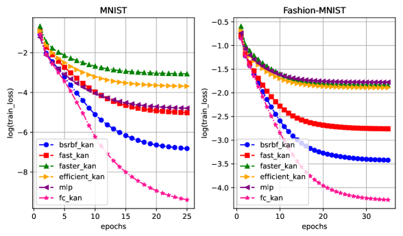
Figure 1: The logarithmic values of training losses for the models over 25 epochs on MNIST and 35 epochs on Fashion-MNIST. A quadratic function is used to combine B-Splines and DoG at the output of FC-KAN.

As shown in Table 1, all models contain a network structure of (784, 64, 10), comprising 784 input neurons, 64 hidden neurons, and 10 output neurons corresponding to the 10 output classes (0-9). Due to the function combinations, FC-KAN has the highest number of parameters, while the MLP has the fewest because it only contains linear transformations over data between layers. The models were trained with 25 epochs on MNIST and 35 epochs on Fashion-MNIST. For KAN models, we use grid_size=5, spline_order=3, and num_grids=8. Other hyperparameters are the same in all models, including batch_size=64, learning_rate=1e-3, weight_decay=1e-4, gamma=0.8, optimize=AdamW, and loss=CrossEntropy.

In FC-KAN models, we combine 2 out of 4 functions: B-splines (denoted as BS), Radial Basis Functions (denoted as RBF, specifically using GRBFs), Difference of Gaussians (denoted as DoG), and base linear transformations (denoted as BASE), to create 6 FC-KAN variants. All variants use a quadratic function representation in the output for the experiments. The FC-KAN models are: FC-KAN (DoG+BS), FC-KAN (DoG+RBF), FC-KAN (DoG+BASE), FC-KAN (BS+RBF), FC-KAN (BS+BASE), and FC-KAN (RBF+BASE).

4.2 Model Performance

Figure 1 shows the training losses, represented on a logarithmic scale, for MLP and KAN models on the MNIST and Fashion-MNIST datasets. The loss performance of each model was evaluated based on an independent training run. FC-KAN consistently achieves the lowest training losses across both datasets, followed by BSRBF-KAN due to its fast convergence feature. In contrast, Faster-KAN records the highest training loss on MNIST, while MLP performs similarly on Fashion-MNIST.

Table 2: The average metric values in 5 training runs on MNIST and Fashion-MNIST. FC-KAN models use a quadratic function representation to combine outputs.

Dataset	Model	Train. Acc.	Val. Acc.	F1	Time (seconds)
MNIST	BSRBF-KAN	100.00 ± 0.00	97.59 ± 0.02	97.56 ± 0.02	211.5
	FastKAN	99.98 ± 0.01	97.47 ± 0.05	97.43 ± 0.05	164.47
	FasterKAN	98.72 ± 0.02	97.69 ± 0.04	97.66 ± 0.04	161.88
	EfficientKAN	99.40 ± 0.10	97.34 ± 0.05	97.30 ± 0.05	184.5
	MLP	99.82 ± 0.08	97.74 ± 0.07	97.71 ± 0.07	146.58
	FC-KAN (DoG+BS)	100.00 ± 0.00	97.91 ± 0.05	97.88 ± 0.05	263.29
	FC-KAN (DoG+RBF)	100.00 ± 0.00	97.83 ± 0.04	97.81 ± 0.04	244.26
	FC-KAN (DoG+BASE)	99.94 ± 0.04	97.81 ± 0.03	97.78 ± 0.03	234.13
	FC-KAN (BS+RBF)	99.95 ± 0.03	97.74 ± 0.04	97.71 ± 0.04	234.07
	FC-KAN (BS+BASE)	99.96 ± 0.02	97.78 ± 0.03	97.75 ± 0.03	235.04
	FC-KAN (RBF+BASE)	99.97 ± 0.02	97.79 ± 0.03	97.76 ± 0.03	228.16
Fashion-MNIST	BSRBF-KAN	99.34 ± 0.04	89.38 ± 0.06	89.36 ± 0.06	276.75
	FastKAN	98.25 ± 0.07	89.40 ± 0.08	89.35 ± 0.08	208.68
	FasterKAN	94.41 ± 0.03	89.31 ± 0.03	89.25 ± 0.02	220.7
	EfficientKAN	94.81 ± 0.09	88.98 ± 0.07	88.91 ± 0.08	247.85
	MLP	94.14 ± 0.04	88.94 ± 0.05	88.88 ± 0.05	200.28
	FC-KAN (DoG+BS)	99.54 ± 0.13	89.99 ± 0.09	89.93 ± 0.08	369.2
	FC-KAN (DoG+RBF)	99.68 ± 0.08	89.93 ± 0.07	89.87 ± 0.07	339.51
	FC-KAN (DoG+BASE)	98.24 ± 0.55	89.81 ± 0.07	89.74 ± 0.07	326.38
	FC-KAN (BS+RBF)	98.58 ± 0.43	89.72 ± 0.07	89.67 ± 0.06	327.49
	FC-KAN (BS+BASE)	98.81 ± 0.35	89.75 ± 0.06	89.70 ± 0.06	327.31
	FC-KAN (RBF+BASE)	98.97 ± 0.30	89.74 ± 0.05	89.69 ± 0.05	318.95
Train. Acc = Training Accuracy, Val. Acc. = Validation Accuracy
BASE = linear transformations, BS = B-splines, DoG = Difference of Gaussians, RBF = Radial Basis Functions

In general, FC-KAN models outperformed others on MNIST and Fashion-MNIST but require more training time due to the quadratic function representation for output combination, as shown in Table 2. This trade-off between training time and model performance is considered reasonable. The best-performing model is FC-KAN (DoG+BS), which achieved a validation accuracy of 97.91% on MNIST and 89.99% on Fashion-MNIST. Although it has the lowest performance on Fashion-MNIST, the MLP model has the fastest training time and shows competitive performance on MNIST, even outperforming BSRBF-KAN, FastKAN, FasterKAN, and EfficientKAN on this dataset.

BSRBF-KAN, FC-KAN (DoG+BS), and FC-KAN (DoG+RBF) exhibit the best convergence on MNIST, while FC-KAN (DoG+RBF) performs the best on Fashion-MNIST, followed by FC-KAN (DoG+BS) and BSRBF-KAN. We observe that fast convergence is achieved in KAN models that incorporate function combinations rather than relying on single functions. This finding is important to consider when designing KANs with a focus on achieving rapid convergence.

4.3 Comparison of Combination Types

While employing a quadratic function representation for the output of FC-KAN, we are also interested in exploring how different output combination methods affect model performance. In this experiment, we use FC-KAN (DoG+BS) with several output combination methods: sum, element-wise product, addition of sum and element-wise product, quadratic function representation, and concatenation.

Table 3: The performance of FC-KAN (DoG+BS) using different output combination methods.

Dataset	Combined Type	Train. Acc.	Val. Acc.	F1	Time (seconds)
MNIST	Sum	100.00 ± 0.00	97.61 ± 0.04	97.58 ± 0.04	247.12
	Product	100.00 ± 0.00	97.59 ± 0.07	97.56 ± 0.07	247.5
	Sum + Product	100.00 ± 0.00	97.73 ± 0.04	97.70 ± 0.04	244.95
	Quadratic Function	100.00 ± 0.00	97.91 ± 0.05	97.88 ± 0.05	263.29
	Concatenation	99.64 ± 0.07	97.20 ± 0.02	97.16 ± 0.02	250.03
Fashion-MNIST	Sum	99.39 ± 0.03	89.56 ± 0.07	89.55 ± 0.09	346.21
	Product	99.50 ± 0.05	89.95 ± 0.08	89.90 ± 0.08	345.85
	Sum + Product	99.56 ± 0.05	89.89 ± 0.13	89.84 ± 0.13	349.4
	Quadratic Function	99.54 ± 0.13	89.99 ± 0.09	89.93 ± 0.08	369.2
	Concatenation	95.27 ± 0.05	89.09 ± 0.04	89.01 ± 0.04	345.35
Train. Acc = Training Accuracy, Val. Acc. = Validation Accuracy

From the results in Table 3, the quadratic function best represents the combination output and outperforms other combinations, although its models require more training time. Meanwhile, the output combination by concatenation shows the worst results. In MNIST, the addition of sum and element-wise product demonstrates very competitive performance while requiring the least training time. Except for concatenation, the other four combinations can easily achieve 100% training accuracy. In Fashion-MNIST, the element-wise product combination is only surpassed by the quadratic function, but it takes 6.3% less training time.

5 Limitation

Although FC-KAN is designed to utilize data combinations in low-dimensional layers, our experiments applied it only to the output layer, considered a low-dimensional layer in a network with the structure (784, 64, 10). As a result, the impact of these combinations on model performance in deeper network architectures with low-dimensional layers remains unclear. Another limitation is the number of parameters in the models. In the experiments, the MLP used the fewest parameters within the same network structure (784, 64, 10) compared to other models. We are also interested in how MLP would perform relative to KAN models if they have the same number of parameters. According to Yu et al. [31], MLP generally outperforms KAN models, except in tasks involving symbolic formula representation.

We also question whether the model’s performance would improve if data combinations were applied in all layers, rather than just low-dimensional layers, assuming that device memory constraints are not an issue in data multiplications. Finally, since FC-KAN has only been tested on two datasets, MNIST and Fashion-MNIST, more datasets should be used to properly evaluate its effectiveness. In short, these limitations can be addressed by designing network structures that integrate low-dimensional data and evaluating them across various problems or through additional experiments for greater clarity.

6 Conclusion

We introduced FC-KAN, which uses various popular mathematical functions to represent data features and combines their outputs using different methods, primarily through element-wise operations in low-dimensional layers, to address image classification problems. In the experiments, we designed FC-KAN to combine pairs of functions, such as B-splines, wavelets, and radial basis functions, using several output combinations on the MNIST and Fashion-MNIST datasets. We found that FC-KAN outperformed MLP and other KAN models with the same network structure, although it required more training time. Among the variants, FC-KAN (DoG+BS), which combines the Difference of Gaussians and B-splines with a quadratic function representation in the output, achieved the best results on both datasets. FC-KAN demonstrates promising potential in using function combinations to design KANs and improve model performance. However, there are several aspects, such as exploring other functions and combinations to extract data features for further model enhancement, that we would like to investigate. These will be the focus of our future work.

References

- Liu et al. [2024a] Ziming Liu, Yixuan Wang, Sachin Vaidya, Fabian Ruehle, James Halverson, Marin Soljačić, Thomas Y Hou, and Max Tegmark. Kan: Kolmogorov-arnold networks. arXiv preprint arXiv:2404.19756, 2024a.
- Liu et al. [2024b] Ziming Liu, Pingchuan Ma, Yixuan Wang, Wojciech Matusik, and Max Tegmark. Kan 2.0: Kolmogorov-arnold networks meet science. arXiv preprint arXiv:2408.10205, 2024b.
- Kolmogorov [1957] Andrei Nikolaevich Kolmogorov. On the representation of continuous functions of many variables by superposition of continuous functions of one variable and addition. In Doklady Akademii Nauk, volume 114, pages 953–956. Russian Academy of Sciences, 1957.
- Li [2024] Ziyao Li. Kolmogorov-arnold networks are radial basis function networks. arXiv preprint arXiv:2405.06721, 2024.
- Delis [2024] Athanasios Delis. Fasterkan. https://github.com/AthanasiosDelis/faster-kan/, 2024.
- Bozorgasl and Chen [2024] Zavareh Bozorgasl and Hao Chen. Wav-kan: Wavelet kolmogorov-arnold networks. arXiv preprint arXiv:2405.12832, 2024.
- SS [2024] Sidharth SS. Chebyshev polynomial-based kolmogorov-arnold networks: An efficient architecture for nonlinear function approximation. arXiv preprint arXiv:2405.07200, 2024.
- Ta [2024] Hoang-Thang Ta. Bsrbf-kan: A combination of b-splines and radial basis functions in kolmogorov-arnold networks. arXiv preprint arXiv:2406.11173, 2024.
- Yang et al. [2024] Zhuoqin Yang, Jiansong Zhang, Xiaoling Luo, Zheng Lu, and Linlin Shen. Activation space selectable kolmogorov-arnold networks. arXiv preprint arXiv:2408.08338, 2024.
- Braun and Griebel [2009] Jürgen Braun and Michael Griebel. On a constructive proof of kolmogorov’s superposition theorem. Constructive approximation, 30:653–675, 2009.
- Zhou et al. [2022] Tian Zhou, Jianqing Zhu, Xue Wang, Ziqing Ma, Qingsong Wen, Liang Sun, and Rong Jin. Treedrnet: a robust deep model for long term time series forecasting. arXiv preprint arXiv:2206.12106, 2022.
- Sprecher and Draghici [2002] David A Sprecher and Sorin Draghici. Space-filling curves and kolmogorov superposition-based neural networks. Neural Networks, 15(1):57–67, 2002.
- Köppen [2002] Mario Köppen. On the training of a kolmogorov network. In Artificial Neural Networks—ICANN 2002: International Conference Madrid, Spain, August 28–30, 2002 Proceedings 12, pages 474–479. Springer, 2002.
- Lin and Unbehauen [1993] Ji-Nan Lin and Rolf Unbehauen. On the realization of a kolmogorov network. Neural Computation, 5(1):18–20, 1993.
- Leni et al. [2013] Pierre-Emmanuel Leni, Yohan D Fougerolle, and Frédéric Truchetet. The kolmogorov spline network for image processing. In Image Processing: Concepts, Methodologies, Tools, and Applications, pages 54–78. IGI Global, 2013.
- Lai and Shen [2021] Ming-Jun Lai and Zhaiming Shen. The kolmogorov superposition theorem can break the curse of dimensionality when approximating high dimensional functions. arXiv preprint arXiv:2112.09963, 2021.
- Girosi and Poggio [1989] Federico Girosi and Tomaso Poggio. Representation properties of networks: Kolmogorov’s theorem is irrelevant. Neural Computation, 1(4):465–469, 1989.
- Vitushkin [1954] AG Vitushkin. On hilbert’s thirteenth problem. In Dokl. Akad. Nauk SSSR, volume 95, pages 701–704, 1954.
- Kůrková [1991] Věra Kůrková. Kolmogorov’s theorem is relevant. Neural computation, 3(4):617–622, 1991.
- Dhiman [2024] Vikas Dhiman. Kan: Kolmogorov–arnold networks: A review. https://vikasdhiman.info/reviews/KAN_a_review.pdf, 2024.
- De Boor [1972] Carl De Boor. On calculating with b-splines. Journal of Approximation theory, 6(1):50–62, 1972.
- Abueidda et al. [2024] Diab W Abueidda, Panos Pantidis, and Mostafa E Mobasher. Deepokan: Deep operator network based on kolmogorov arnold networks for mechanics problems. arXiv preprint arXiv:2405.19143, 2024.
- Bhattacharjee [2024] Subhransu S. Bhattacharjee. Torchkan: Simplified kan model with variations. https://github.com/1ssb/torchkan/, 2024.
- Xu et al. [2024] Jinfeng Xu, Zheyu Chen, Jinze Li, Shuo Yang, Wei Wang, Xiping Hu, and Edith C-H Ngai. Fourierkan-gcf: Fourier kolmogorov-arnold network–an effective and efficient feature transformation for graph collaborative filtering. arXiv preprint arXiv:2406.01034, 2024.
- Seydi [2024] Seyd Teymoor Seydi. Unveiling the power of wavelets: A wavelet-based kolmogorov-arnold network for hyperspectral image classification. arXiv preprint arXiv:2406.07869, 2024.
- Teymoor Seydi [2024] Seyd Teymoor Seydi. Exploring the potential of polynomial basis functions in kolmogorov-arnold networks: A comparative study of different groups of polynomials. arXiv e-prints, pages arXiv–2406, 2024.
- Chernov [2020] Andrei Vladimirovich Chernov. Gaussian functions combined with kolmogorov’s theorem as applied to approximation of functions of several variables. Computational Mathematics and Mathematical Physics, 60:766–782, 2020.
- Schmidt-Hieber [2021] Johannes Schmidt-Hieber. The kolmogorov–arnold representation theorem revisited. Neural networks, 137:119–126, 2021.
- Deng [2012] Li Deng. The mnist database of handwritten digit images for machine learning research [best of the web]. IEEE signal processing magazine, 29(6):141–142, 2012.
- Xiao et al. [2017] Han Xiao, Kashif Rasul, and Roland Vollgraf. Fashion-mnist: a novel image dataset for benchmarking machine learning algorithms. arXiv preprint arXiv:1708.07747, 2017.
- Yu et al. [2024] Runpeng Yu, Weihao Yu, and Xinchao Wang. Kan or mlp: A fairer comparison. arXiv preprint arXiv:2407.16674, 2024.