Decoding finger velocity from cortical spike trains with recurrent spiking neural networks

Abstract

Invasive cortical brain-machine interfaces can significantly improve the life quality of motor-impaired patients. Nonetheless, externally mounted pedestals pose an infection risk, which calls for fully implanted systems. Such systems, however, must meet strict latency and energy constraints while providing reliable decoding performance. While recurrent spiking neural networks are ideally suited for ultra-low-power, low-latency processing on neuromorphic hardware, it is unclear whether they meet the above requirements. To address this question, we trained RSNNs to decode finger velocity from cortical spike trains of two macaque monkeys. First, we found that a large RSNN model outperformed existing feed-forward spiking neural networks and artificial neural networks in terms of their decoding accuracy. We next developed a tiny RSNN with a smaller memory footprint, low firing rates, and sparse connectivity. Despite its reduced computational requirements, the resulting model performed substantially better than existing SNN and ANN decoders. Our results thus demonstrate that RSNNs offer competitive CST decoding performance under tight resource constraints and are promising candidates for fully implanted ultra-low-power BMIs with the potential to revolutionize patient care.

I Introduction

BMI enable direct communication between biological neural networks and external devices [1]. Significant progress has been made in invasive BMI technology, allowing volitional control of robotic arms [2, 3] and text generation for communication [4, 5, 6, 7]. Despite rapid improvements in decoding performance, a central challenge persists: the risk of wound infection due to externally mounted pedestals. Fully implanted BMIs offer a potential solution [8, 9, 10], but introduce new constraints on energy consumption and heat dissipation of the implants. For instance, the American Association of Medical Instrumentation guidelines stipulate that chronically implanted medical devices must not increase tissue temperature by more than 1°C [11]. Consequently, fully implanted BMIs require a computational substrate capable of delivering reliable and accurate decoding performance within strict latency and power limits.

SNN offer an attractive solution for fully implanted BMIs. Their spike-based communication minimizes pre-processing requirements for CSTs and makes them suitable for ultra-low power, low-latency neuromorphic hardware [12, 13]. Several studies have explored the decoding abilities of feed-forward SNNs [8, 9, 10, 14], but these models achieved only moderate decoding performance on standard benchmarks, such as decoding finger velocity from monkeys performing a reaching task [15]. For instance, [10] developed an energy-efficient feed-forward SNN, which achieved only moderate decoding accuracy ( coefficient of determination ($R^{2}$) value of 0.45 averaged across two CST recording sessions). The community-driven NeuroBench project [8] proposed additional SNN models for CST decoding, termed SNN and SNN_Flat, achieving average $R^{2}$ values of $0.58$ and $0.63$, respectively. However, the increased decoding accuracy of the SNN_Flat model comes at a substantial energy cost. Consequently, existing feed-forward SNN models fail to simultaneously meet decoding performance and energy efficiency requirements.

RSNN, which go beyond simple feed-forward architectures, remain largely unexplored for fully implanted BMIs applications. Here, we address this gap by investigating the decoding performance and energy efficiency of RSNNs on finger velocity decoding from CSTs in monkeys [15].

II Methods

To study the decoding performance of RSNNs, we iteratively developed two distinct model architectures: First, we explored the maximum decoding performance achievable through end-to-end training of RSNNs, which we refer to as “bigRSNN”. Second, to balance decoding performance and energy efficiency for fully implanted BMI applications, we developed a lightweight “tinyRSNN”, reducing the number of model parameters by several orders of magnitude.

II-A Network architectures

Both models consist of a spiking input layer matching the number of electrode channels in the CST recording, followed by a single recurrent layer of standard leaky integrate-and-fire (LIF) neurons, and a readout layer of non-spiking leaky integrator (LI) neurons (Fig. 1A). All LIF and LI units in the network feature synaptic and membrane dynamics with learnable, unit-specific synaptic and membrane time constants [16]. During training, we optimized the membrane potential of the readout units to match the measured monkey finger velocities. The two network models primarily differ in the size of their hidden and readout layers, with tinyRSNN additionally incorporating techniques that encourage activity and connection sparsity (see Section II-D).

To explore the upper limit of decoding capabilities, we designed bigRSNN with 1024 units in the hidden layer. Mimicking ensemble methods that have been proven successful in machine learning [17], we incorporated a readout layer with five readout heads. Each head consists of two non-spiking LI neurons corresponding to finger velocities along the X and Y axes, respectively. These readout heads were allowed to have different synaptic and membrane dynamics. The final predicted finger velocities were determined by averaging the predictions across all readout heads.

To better accommodate the resource-constrained setting of realistic BMI applications, we designed tinyRSNN with a limited hidden layer size of 64 recurrently connected LIF neurons. In contrast to the multi-head readout strategy of bigRSNN, tinyRSNN employs a simpler readout layer with only two LI units, one each for X and Y directions.

II-B Data pre-processing

Both models were trained on multi-unit activity (MUA) from CST recordings obtained over multiple sessions from two macaque monkeys, Indy and Loco [15, 14] (Fig. 1B). For each session, we split the data into 65% training, 10% validation, and 25% test sets. We discretized input spikes into 4 ms long bins, each representing one time step for the model. To enable mini-batch training, we divided the training and validation data into overlapping two-second samples (500 time steps per sample). In contrast, we presented the test data to the models continuously, time step by time step as a single long sample, mimicking real-time processing conditions.

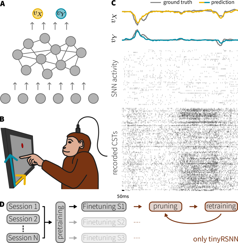
Figure 1: Setup and example network activity. A) Schematic of the RSNN network architecture. B) The publicly available dataset consists of CSTs recorded from two macaque monkeys performing a self-paced reaching task using chronically implanted electrodes. Recording sites were either in the primary motor cortex (M1) (Indy) or in M1 and the primary sensory cortex (S1) (Loco) [15]. C) Example network activity for tinyRSNN. Bottom: Spike raster of recorded CSTs which serves as input to the model. Middle: Spike raster of the recurrent hidden layer activity. Top: Membrane potentials of the readout units (colored) and the ground-truth finger velocities (gray). D) Schematic of the training curriculum. For each monkey, we pre-trained on all available sessions, with subsequent session-wise fine-tuning. For tinyRSNN, we further added iterative pruning at the end of the curriculum.

II-C Training

The training process for bigRSNN and tinyRSNN followed the same structured approach: We initialized models in the fluctuation-driven regime [18]. For each monkey, we first pre-trained the models for 100 epochs on concatenated and shuffled data samples from all available sessions [15]. After pre-training, we independently fine-tuned the models for 200 epochs on each of three sessions per monkey [14] (cf. Fig. 1D). For each session, we trained five models with different parameter initializations. All SNNs were trained using surrogate gradient descent [19] to minimize the root mean squared error between predicted and target finger velocities. We used the SMORMS3 optimizer [20, 18] with a cosine learning rate schedule to accelerate learning. To avoid silent neurons during training, we added a homeostatic activity regularization term to the loss function [18]. Finally, we applied dropout with $p=0.3$ to the input and hidden layers to mitigate overfitting. Detailed hyperparameters and training settings for both models can be found in the configuration files in our GitHub repository. All simulations were run in Python version 3.10.12 using custom code based on the Stork SNN simulator [18] and PyTorch [21].

II-D Activity regularization and pruning

We further optimized the tinyRSNN model for energy efficiency through three approaches: First, we encouraged sparse neuronal activity by incorporating an activity regularization term to the loss function, which imposes an upper bound on the average firing rate of the hidden layer [18]. Second, we implemented an iterative pruning strategy for all synaptic weights to reduce the number of parameters and synaptic operations. Following fine-tuning, we initially pruned the 40% of the weights with the smallest magnitude and trained the remaining weights for an additional 100 epochs. We then iteratively pruned an additional 10% of weights and fine-tuned, as long as the $R^{2}$ value stayed above a predefined threshold, i.e. 2% below the original accuracy before pruning. Once this threshold was reached, we reduced the pruning rate to 5% and continued until the $R^{2}$ value fell below the threshold again (Fig. 1D). Finally, to further reduce the memory footprint of the network, we converted all model parameters and buffers to half precision after training.

III Results

We assessed the trained models’ decoding performance and computational complexity using the following metrics as suggested by the NeuroBench project [8]: For decoding performance, we calculated the $R^{2}$ between predicted and observed finger velocities on the test dataset. To evaluate computational cost, we measured the total memory footprint of the networks in bytes, their activation and connection sparsity, and the number of synaptic operations used by the models. The latter was determined using the total number of operations during inference (Dense) and the total number of effective accumulate (AC) and multiply-and-accumulate (MAC) operations. Notably, as both models are pure SNN models without normalization layers, they perform no effective MAC operations. If not stated otherwise, we report averages across five different random initializations $\pm$ standard deviation.

III-A Decoding performance

We first assessed the decoding performance of tinyRSNN and bigRSNN and found that both models provided good estimates of finger velocity (Fig. 2). In particular, both models outperformed previously published feed-forward SNN decoders (see Table I), as well as conventional ANNs trained on the same dataset (average $R^{2}$ values: ANN: 0.579, ANN_Flat: 0.615 [8]). As anticipated, the less constrained bigRSNN exhibited superior performance compared to tinyRSNN across all sessions (Table I, Fig. 2B). These results suggest that the incorporation of recurrent connections enhances the processing capabilities of SNNs, conferring advantages in CST decoding tasks.

Table I: Session Specific $R^{2}$ Scores Compared to Baseline Models.

Session	Baseline [8]		Ours
	SNN	SNN_Flat	tinyRSNN	bigRSNN
I1	$0.677$	$0.697$	$0.752\pm 0.003$	$0.770\pm 0.003$
I2	$0.501$	$0.577$	$0.545\pm 0.004$	$0.585\pm 0.012$
I3	$0.599$	$0.652$	$0.746\pm 0.007$	$0.772\pm 0.006$
L1	$0.571$	$0.623$	$0.622\pm 0.003$	$0.698\pm 0.006$
L2	$0.515$	$0.568$	$0.608\pm 0.006$	$0.629\pm 0.008$
L3	$0.620$	$0.681$	$0.690\pm 0.006$	$0.734\pm 0.005$
Mean	$\mathbf{0.581}$	$\mathbf{0.633}$	$\mathbf{0.660\pm 0.002}$	$\mathbf{0.698\pm 0.002}$

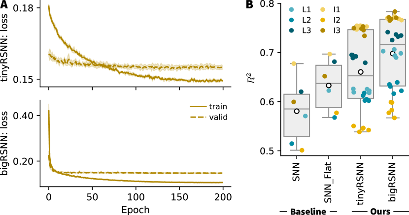
Figure 2: Learning and decoding performance of the RSNN models. A) Learning curves for the tinyRSNN (top) and the bigRSNN (bottom) for session I3. B) $R^{2}$ values for ours and the baseline models (SNN, SNN_Flat [8]). Each point corresponds to a network with a different random initialization; colors indicate the different sessions.

Table II: Computational Cost of tinyRSNN Compared to Resource-Efficient Baseline Models. Bold: Best Values.

		Baseline [8]		Ours
		SNN	ANN	tinyRSNN
Memory footprint [bytes]		$29248$	$27160$	$\mathbf{27144\pm 0}$
Connection Sparsity		$0$	$0$	$\mathbf{0.45\pm 0.01}$
Activation Sparsity		$\mathbf{0.9976}$	$0.6755$	$0.9836\pm 0.0001$
SynOps	Dense	$7300$	$\mathbf{6237}$	$13440\pm 0$
	Effective MACs	$\mathbf{0}$	$4967$	$\mathbf{0\pm 0}$
	Effective ACs	$414$	$\mathbf{0}$	$304\pm 8$
Effective Energy Ratio		$1.36$	$506.50$	$\mathbf{1}$

III-B Computational complexity of the tinyRSNN model

Next, we investigated the memory footprint and computational cost of the models. We found that tinyRSNN had a smaller memory footprint and higher connection sparsity compared to feed-forward resource-optimized SNN decoders [8], despite its superior decoding performance (cf. Table II). The tinyRSNN model uses fewer ACs on average, a direct consequence of activity regularization and pruning. More precisely, it featured an average connection sparsity of 45% and an average activation sparsity of 98.36% (Table II; cf. Tables III and IV for session-specific results). To estimate energy consumption on optimized hardware, we computed the effective energy ratio [22, 23]. By this metric, tinyRSNN reduced energy consumption by 26.6% compared to the SNN decoder from [8]. Furthermore, it requires approximately 500 times less energy than a traditional ANN decoder trained on the same task [8] (see Table II). These results suggest that small RSNN models can effectively leverage activity regularization and synaptic pruning strategies to substantially reduce computational costs while maintaining high decoding performance.

IV Discussion & Conclusion

We developed two RSNN models for decoding finger velocities from CSTs and evaluated their decoding performance and energy efficiency. Our bigRSNN model significantly improved decoding performance compared to existing models. Additionally, we introduced the tinyRSNN model, tailored for fully implanted BMI applications. This model was designed to find a Pareto optimum between decoding accuracy and energy efficiency. Our work demonstrates that, through the application of suitable training techniques, the computational complexity of RSNNs can be remarkably reduced. By combining small layer sizes, activity regularization, and synaptic pruning, we substantially reduced the computational requirements while hardly impacting decoding performance. Notably, tinyRSNN exhibits considerable performance improvements over existing models with comparable resource requirements.

While we have demonstrated promising performance improvements, several questions remain open. For instance, the specific roles of individual factors, such as recurrent connections, in driving these improvements remain unclear. A detailed analysis of their impact is a key area for future work. Recent work has highlighted synaptic delays as an architectural feature that can enhance SNN performance [24, 25]. These delays may also allow for reduced memory requirements while being amenable to efficient hardware implementations [26, 27]. In future work, we will explore whether incorporating synaptic delays could further improve CSTs decoding. Although tinyRSNN constitutes a parsimonious model that should in principle be suitable for a hardware implementation, we have not formally shown its performance gains on physical hardware. We intend to implement this model on suitable neuromorphic processors in future work, a crucial step toward realizing practical, fully implanted BMIs.

In conclusion, RSNNs have proven to be competitive models for real-time CSTs decoding that outperform existing models. Moreover, we have shown that their computational complexity can be substantially reduced through suitable training strategies, with minimal impact on accuracy. These advancements bring us closer to the next generation of efficient, high-performance neural decoders for implantable BMIs applications, with the potential to elevate the standard of patient care.

V Acknowledgments

This work was supported by STI 2030-Major Projects (2022ZD0208604, 2021ZD0200300), ZJU Doctoral Graduate Academic Rising Star Development Program (2023059), EU’s Horizon Europe Research and Innovation Programme (Grant Agreement No. 101070374, CONVOLVE) funded through SERI (Ref. 1131-52302), the Swiss National Science Foundation (Grant Number PCEFP3_202981), and the Novartis Research Foundation.

Table III: Quantification of Memory Footprint and Sparsity.

	Session	tinyRSNN	bigRSNN
Memory footprint [bytes]	I1 - I3	$21\,000$	$4\,636\,752$
	L1 - L3	$33\,288$	$5\,029\,968$
	Mean	$27\,144$	$4\,833\,360$
Connection Sparsity	I1	$0.47\pm 0.02$	$0$
	I2	$0.45\pm 0.03$	$0$
	I3	$0.50\pm 0.00$	$0$
	L1	$0.44\pm 0.04$	$0$
	L2	$0.42\pm 0.02$	$0$
	L3	$0.45\pm 0.03$	$0$
	Mean	$\mathbf{0.45\pm 0.01}$	$\mathbf{0}$
Activation Sparsity	I1	$0.9838\pm 0.0004$	$0.9622\pm 0.0002$
	I2	$0.9853\pm 0.0003$	$0.9718\pm 0.0006$
	I3	$0.9842\pm 0.0002$	$0.9721\pm 0.0002$
	L1	$0.9831\pm 0.0001$	$0.9677\pm 0.0012$
	L2	$0.9832\pm 0.0002$	$0.9674\pm 0.0010$
	L3	$0.9820\pm 0.0003$	$0.9686\pm 0.0014$
	Mean	$\mathbf{0.9836\pm 0.0001}$	$\mathbf{0.9683\pm 0.0005}$

Table IV: Session Specific and Average Synaptic Operations.

	Session	tinyRSNN	bigRSNN
Dense	I1 - I3	$10\,368$	$1\,157\,120$
	L1 - L3	$16\,512$	$1\,255\,424$
	Mean	$13\,440$	$1\,206\,272$
Effective ACs	I1	$299\pm 14$	$$48\,096$\pm 254$
	I2	$197\pm 12$	$$34\,837$\pm 659$
	I3	$143\pm 2$	$$33\,289$\pm 181$
	Mean Indy	$\mathbf{213\pm 4}$	$\mathbf{$38\,741$\pm$190$}$
	L1	$354\pm 28$	$$44\,664$\pm$1258$$
	L2	$404\pm 20$	$$45\,945$\pm$1097$$
	L3	$427\pm 28$	$$45\,189$\pm$1437$$
	Mean Loco	$\mathbf{395\pm 19}$	$\mathbf{$45\,266$\pm$1056$}$

References

- [1] Ujwal Chaudhary, Niels Birbaumer and Ander Ramos-Murguialday “Brain–computer interfaces for communication and rehabilitation” In Nature Reviews Neurology 12.9 Nature Publishing Group UK London, 2016, pp. 513–525
- [2] Leigh R Hochberg et al. “Reach and grasp by people with tetraplegia using a neurally controlled robotic arm” In Nature 485.7398 Nature Publishing Group UK London, 2012, pp. 372–375
- [3] Sharlene N Flesher et al. “A brain-computer interface that evokes tactile sensations improves robotic arm control” In Science 372.6544 American Association for the Advancement of Science, 2021, pp. 831–836
- [4] Chethan Pandarinath et al. “High performance communication by people with paralysis using an intracortical brain-computer interface” In elife 6 eLife Sciences Publications, Ltd, 2017, pp. e18554
- [5] Francis R Willett et al. “High-performance brain-to-text communication via handwriting” In Nature 593.7858 Nature Publishing Group UK London, 2021, pp. 249–254
- [6] David A. Moses et al. “Neuroprosthesis for Decoding Speech in a Paralyzed Person with Anarthria” In New England Journal of Medicine 385.3 Massachusetts Medical Society, 2021, pp. 217–227 DOI: 10.1056/NEJMoa2027540
- [7] Nicholas S Card et al. “An accurate and rapidly calibrating speech neuroprosthesis” In The New England journal of medicine 391.7 Massachusetts Medical Society, 2024, pp. 609–618 DOI: 10.1056/NEJMoa2314132
- [8] Jason Yik et al. “NeuroBench: A Framework for Benchmarking Neuromorphic Computing Algorithms and Systems” In NeuroBench 2304.04640 arXiv.org, 2024 DOI: 10.48550/arXiv.2304.04640
- [9] Elijah A. Taeckens and Sahil Shah “A Spiking Neural Network with Continuous Local Learning for Robust Online Brain Machine Interface” In Journal of Neural Engineering 20.6 IOP Publishing, 2024, pp. 066042 DOI: 10.1088/1741-2552/ad1787
- [10] Jiawei Liao et al. “An energy-efficient spiking neural network for finger velocity decoding for implantable brain-machine interface” In 2022 IEEE 4th International Conference on Artificial Intelligence Circuits and Systems (AICAS), 2022, pp. 134–137 IEEE
- [11] Patrick D Wolf and WM Reichert “Thermal considerations for the design of an implanted cortical brain–machine interface (BMI)” In Indwelling Neural Implants: Strategies for Contending with the In Vivo Environment CRC Press/Taylor & Francis Boca Raton, 2008, pp. 33–38
- [12] Giacomo Indiveri et al. “Neuromorphic Silicon Neuron Circuits” In Frontiers in Neuroscience 5 Frontiers, 2011 DOI: 10.3389/fnins.2011.00073
- [13] Elisa Donati and Giacomo Valle “Neuromorphic hardware for somatosensory neuroprostheses” Number: 1 Publisher: Nature Publishing Group In Nature Communications 15.1, 2024, pp. 556 DOI: 10.1038/s41467-024-44723-3
- [14] Biyan Zhou et al. “IEEE BioCAS 2024 Grand Challenge on Neural Decoding for Motor Control of Non-Human Primates” IEEE Dataport, 2024 DOI: 10.21227/bp1f-te92
- [15] Joseph E. O’Doherty, Mariana M.. Cardoso, Joseph G. Makin and Philip N. Sabes “Nonhuman Primate Reaching with Multichannel Sensorimotor Cortex Electrophysiology” Zenodo, 2017 DOI: 10.5281/zenodo.583331
- [16] Nicolas Perez-Nieves, Vincent C.. Leung, Pier Luigi Dragotti and Dan F.. Goodman “Neural Heterogeneity Promotes Robust Learning” In Nature Communications 12.1, 2021, pp. 5791 DOI: 10.1038/s41467-021-26022-3
- [17] Lior Rokach “Ensemble Methods for Classifiers” In Data Mining and Knowledge Discovery Handbook Boston, MA: Springer US, 2005, pp. 957–980 DOI: 10.1007/0-387-25465-X˙45
- [18] Julian Rossbroich, Julia Gygax and Friedemann Zenke “Fluctuation-Driven Initialization for Spiking Neural Network Training” In Neuromorphic Computing and Engineering 2.4, 2022, pp. 044016 DOI: 10.1088/2634-4386/ac97bb
- [19] Emre O. Neftci, Hesham Mostafa and Friedemann Zenke “Surrogate Gradient Learning in Spiking Neural Networks: Bringing the Power of Gradient-based optimization to spiking neural networks” In IEEE Signal Processing Magazine 36.6, 2019, pp. 51–63 DOI: 10.1109/MSP.2019.2931595
- [20] Simon Funk “RMSprop Loses to SMORMS3 - Beware the Epsilon!”, https://sifter.org/simon/journal/20150420.html, 2015
- [21] Adam Paszke et al. “PyTorch: An Imperative Style, High-Performance Deep Learning Library” In Advances in Neural Information Processing Systems 32 Curran Associates, Inc., 2019, pp. 8024–8035
- [22] Bojian Yin, Federico Corradi and Sander M. Bohté “Accurate and Efficient Time-Domain Classification with Adaptive Spiking Recurrent Neural Networks” In Nature Machine Intelligence 3.10 Nature Publishing Group, 2021, pp. 905–913 DOI: 10.1038/s42256-021-00397-w
- [23] Mark Horowitz “1.1 Computing’s Energy Problem (and What We Can Do about It)” In 2014 IEEE International Solid-State Circuits Conference Digest of Technical Papers (ISSCC), 2014, pp. 10–14 DOI: 10.1109/ISSCC.2014.6757323
- [24] Malu Zhang et al. “Supervised learning in spiking neural networks with synaptic delay-weight plasticity” In Neurocomputing 409 Elsevier, 2020, pp. 103–118
- [25] Ilyass Hammouamri, Ismail Khalfaoui-Hassani and Timothée Masquelier “Learning Delays in Spiking Neural Networks Using Dilated Convolutions with Learnable Spacings” arXiv, 2023 arXiv:2306.17670 [cs]
- [26] Simone D’Agostino et al. “DenRAM: Neuromorphic Dendritic Architecture with RRAM for Efficient Temporal Processing with Delays” In Nature Communications 15.1 Nature Publishing Group, 2024, pp. 3446 DOI: 10.1038/s41467-024-47764-w
- [27] Filippo Moro, Pau Vilimelis Aceituno, Laura Kriener and Melika Payvand “The Role of Temporal Hierarchy in Spiking Neural Networks” arXiv, 2024 arXiv:2407.18838 [cs]