A Causal Framework for Evaluating Heterogeneous Policy Mechanisms Using Difference-in-Differences

Abstract

In designing and evaluating public policies, policymakers and researchers often hypothesize about the mechanisms through which a policy may affect a population and aim to assess these mechanisms in practice. For example, when studying an excise tax on sweetened beverages, researchers might explore how cross-border shopping, economic competition, and store-level price changes differentially affect store sales. However, many policy evaluation designs, including the difference-in-differences (DiD) approach, traditionally target the average effect of the intervention rather than the underlying mechanisms. Extensions of these approaches to evaluate policy mechanisms often involve exploratory subgroup analyses or outcome models parameterized by mechanism-specific variables. However, neither approach studies the mechanisms within a causal framework, limiting the analysis to associative relationships between mechanisms and outcomes, which may be confounded by differences among sub-populations exposed to varying levels of the mechanisms. Therefore, rigorous mechanism evaluation requires robust techniques to adjust for confounding and accommodate the interconnected relationship between stores within competitive economic landscapes. In this paper, we present a framework for evaluating policy mechanisms by studying Philadelphia beverage tax. Our approach builds on recent advancements in causal effect curve estimators under DiD designs, offering tools and insights for assessing policy mechanisms complicated by confounding and network interference.

1 Introduction

Public policies play a crucial role in shaping population health and economic outcomes [21]. In recent years, excise taxes on sweetened beverages have become a popular tool for generating revenue for government initiatives and promoting healthier behaviors in both the United States, where taxes have been implemented across 8 cities, and globally, where taxes are implemented nationally in over 100 countries [10]. While there is significant evidence supporting revenue generation and reductions in beverage sales in regions implementing the tax, the degree of tax efficacy has varied considerably across regions with little understood regarding these sources of heterogeneity [2]. For example, Philadelphia experienced some of the most pronounced effects among U.S. cities, with several hypotheses cited for increased price sensitivity including high levels of cross-border shopping and tax-related advertisements [22]. Understanding the specific mechanisms driving policy effects is a critical area of research for assessing policy effectiveness, heterogeneity, and equitability with regards to intended outcomes not only for beverage excise taxes but also for many other public policies [17].

We can evaluate these mechanisms by leveraging data on how sub-populations were differentially exposed to these mechanisms. For example, by examining store proximity to non-taxed regions, we can assess how cross-border shopping accessibility and the characteristics of populations near these borders influence tax efficacy. Additionally, since the tax was levied on manufacturers instead of consumers, Philadelphia stores had the discretion to adjust their prices accordingly. This heterogeneity allows us to investigate economic mechanisms such as whether store-level pricing decisions and nearby price competition are influencing tax efficacy. To rigorously evaluate these mechanisms, we must determine the effect heterogeneity attributable to a specific mechanism after adjusting for effect heterogeneity due to other mechanisms and confounding factors.

Methodologists frequently employ the difference-in-differences (DiD) approach to estimate the effects of policy interventions in observational studies, as its design inherently adjusts for observed and unobserved confounding factors that affect outcomes constantly over time and differ between groups implementing and not implementing a policy [3]. Further developments have also been made to adjust for observed confounding differences between the treated and untreated groups that affect outcome trends over time [1, 23]. When evaluating specific mechanisms, researchers typically adopt one of two approaches. The first involves exploratory subgroup analyses, where estimated effect differences between subgroups are then interpreted as associations with subgroup characteristics. While informative, this approach fails to rigorously identify a causal mechanism, as it estimates effects on distinct populations, prohibiting researchers from attributing the true source of effect heterogeneity to the policy mechanism. Additionally, this method often requires subjective clustering of relevant subgroups, increasing the risk of bias-inducing procedures like data-snooping. The second approach involves parameterizing models with terms representing the level of mechanism that a unit is exposed to. Although this approach reduces the need for discretization, it often relies on strong parametric assumptions and is generally insufficient for identifying causal mechanisms without strict no confounding assumptions [6].

Instead, researchers must carefully frame questions pertaining to policy mechanisms from a causal framework to evaluate them rigorously. Recent advances have refined the DiD methodology to evaluate causal effects of continuous exposures while adjusting for confounding differences between intervention groups and between populations receiving different levels of the exposure [12]. Specifically, [12] developed a robust DiD estimator that nonparametrically estimates causal effect curves for continuous exposures, provided that a subset of outcome and propensity score models are well-specified. By leveraging these methodological advancements, we can develop enhanced frameworks to evaluate policy mechanisms while addressing practical challenges like spatial correlation and economic competition.

The need for clear and rigorous frameworks for the stated challenges serves as the motivation for this work. The remainder of the paper is organized as follows: in Section 2, we outline policy-relevant questions for the beverage tax and conceptualize these under hypothetical experiments to provide intuition for the subsequent causal methodology that we employ. Section 3 translates these hypothetical experiments into formal causal estimands before reviewing and extending recent methodologies to evaluate policy mechanisms while addressing relevant practical challenges. Here, we also provide guidance concerning approaches for modeling required nuisance functions and accommodating economic competition between and within regions. In Section 4, we apply our framework to investigate the specific mechanisms of the beverage tax policy enacted in Philadelphia in 2017 and interpret our findings. Finally, we conclude in Section 5 with a discussion on the broader applicability of this framework and suggest directions for future research.

2 Counterfactual Framing of Policy Mechanisms with Hypothetical Experiments

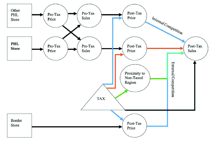
Figure 1: A conceptual diagram of the tax mechanisms that affect sales at a given Philadelphia store.

In this paper, we illustrate our framework by evaluating three key mechanisms through which the tax may affect beverage sales at a Philadelphia store, as conceptually depicted in Figure 1.

First, we examine the cross-border shopping mechanism by assessing the role of proximity to a non-taxed region. In Figure 1, this mechanism is represented by the green-arrowed path, which demonstrates how the tax can affect Philadelphia store sales by shifting some sales to nearby, competitive non-taxed stores. Here, border proximity and non-taxed store prices function jointly to influence sales at a taxed store. To assess the influence of distance to the border on tax effects, we can imagine a hypothetical experiment where all Philadelphia stores are “set” to a fixed distance, $\delta$, from the non-taxed region. Then, we can evaluate the tax effects under various distances, $\delta$, and analyze how effects vary with distance. If we want to evaluate the effect that population composition near the border (e.g., lower socioeconomic status) has on the tax efficacy, we could consider a hypothetical experiment where zip codes are randomly assigned different proximities to the border and compare the tax effect in this setting to the effect under the current zip code arrangement. To operationalize these hypothetical experiments, we will control for differences in post-tax price changes and internal competition that may vary across Philadelphia stores according to border proximity, but not for the effect of external competition, which functions jointly with border proximity.

Second, we examine the mechanism through which stores adjust their beverage prices in response to the tax, depicted by the orange-arrowed path in Figure 1. In theory, stores use information about their consumer base to determine the amount of the tax (1.5 cents per oz.) to pass-through to consumers to optimize overall profits, which may influence the effectiveness of the tax on beverage sales. To assess the impact of this pricing mechanism on tax efficacy, we can imagine a hypothetical experiment where stores are randomly assigned a specific price change, $\delta$. We would then compare the tax effect under this randomized price adjustment to the effect observed when stores independently choose their price changes. We can also consider the hypothetical experiment where all stores are required to change their price by a fixed amount, $\delta$, which may represent alternative policies like if the tax were placed on the consumer. To adequately capture these counterfactual scenarios, we will need to incorporate the downstream effects on both internal and external competition which will differ under counterfactual price changes. Alternatively, we must control for border proximity, which remains constant in this counterfactual context but may confound the observed relationship between price change and sales.

Third, we examine the mechanism by which the tax affects sales through price competition, illustrated by the two blue-arrowed paths. Following awareness of a new tax, consumers may be prone to “shop around” for better prices. In Philadelphia, it is hypothesized that such behaviors may be more prominent due to the high levels of tax-related advertising and the lower socioeconomic status of the population relative to some other implementing cities. To assess the effect of price competition, we can imagine a hypothetical experiment where we fix the minimum beverage price within the neighborhood of each store, $i$, to be $\delta$ cents than the price at store $i$. Then, we could analyze how these tax effects vary based on different levels of price competition to attribute a causal mechanism of logical price competition. To operationalize this hypothetical experiment and isolate the effect of this specific mechanism, we will need to account for the associations between price competition (blue-arrowed paths) and (1) direct price changes (orange-arrowed path) and (2) border proximity (green-arrowed path).

Here, our data demonstrate that store-level trends in beverage sales at Philadelphia pharmacies are associated with lower store-level prices and reduced nearby economic competition within individual zip codes and between adjacent zip codes.

3 Methods

3.1 Notation

Consider the setting where a policy intervention induces a distribution of exposures on the population receiving the intervention. We assume the intervention is introduced between two time-periods, $t=0,1$. Stores, denoted with subscript $i$, serve as the unit of our analysis and are either in the taxed group, $A_{i}=1$, of which there are $n_{1}$, or not, $A_{i}=0$, of which there are $n_{0}=n-n_{1}$. The time-varying tax status at time $t$ is denoted by $Z_{it}=tA_{i}\in\{0,1\}$. In each time period, stores set their prices as $\rho_{it}$.

Analogously, units are differentially exposed to inherent tax mechanisms, which either directly result from the tax (e.g., price change) or become “activated” with the tax (e.g., geographic accessibility to a non-taxed region). We represent exposures to these mechanisms separately as distance to the border, $D_{i}\in\mathbbm{D}$, pass-through rate, $P_{i}=\rho_{i1}-\rho_{i0}\in\mathbbm{P}$, and effective price competition, $h_{it}(\boldsymbol{\rho})\in\mathbbm{H}$. Here, $h_{it}(\boldsymbol{\rho_{t}})$ is a function of all prices in the study, $\boldsymbol{\rho_{t}}$, that we must specify to the represent how consumers think about neighborhood price competition. We separately define the function of all Philadelphia prices as $h_{it}(\boldsymbol{\rho_{t}}|A=1)$. Specifically, this exposure mapping function, introduced by [4], must summarize all exposure that store $i$ receives to price through prices at other stores. In our setting, we specify this as the difference in $\rho_{it}$ and the minimum $\rho_{jt}$ for $j\in\text{neighborhood of }i$, where neighborhoods are defined as adjacent zip-codes.

To distinguish between interventions (binary) and the exposures to mechanisms (continuous), we will often refer to the continuous exposure as a dose. We observe outcomes of interest in each time period, $Y_{it}$. Finally, we denote observed pre-intervention covariates as $\mathbf{X_{i}}$, which we will use to account for covariate effects on outcome trends, although we could also include time-varying covariates assuming time-invariant effects [27].

3.2 Causal Estimands

In this section, we frame the hypothetical interventions contrived in Section 2 as causal parameters, namely contrasts in potential outcomes. Based on the question, we define potential outcomes, $Y_{it}^{(\mathbf{v})}$, according to a vector, $\mathbf{v}$, of interventions and/or mechanisms upon which we would hypothetically intervene. All expectations throughout this work are taken across units $i$ and for simplicity, we omit the unit subscript $i$ within the expectation.

First, we consider a common estimand in policy evaluations, the Average Treatment Effect on the Treated (ATT):

$$ATT:=E[Y_{1}^{(Z_{1}=1)}-Y_{1}^{(Z_{1}=0)}|A=1]$$ (1)

. This estimand asks “What would be the average difference in post-tax (i.e., 2017) sales at Philadelphia stores had all stores been (1) intervened on (i.e., taxed) vs. (2) given the control exposure (i.e., not taxed)?”

Second, we consider an effect curve explored in [12], denoted the Average Dose Effect on the Treated (ADT). Let $\mathbf{M}$ represent a possibly multi-dimensional measure of exposure to a mechanism of interest. For example, this may represent distance to the border, $\mathbf{M_{i}}=D_{i}$, or a two-dimensional representation of price change and subsequent economic competition, $\mathbf{M_{i}}=(P_{i},h_{i1}(\boldsymbol{\rho_{1}}))$. Then, the ADT can be denoted as:

$$ADT(\boldsymbol{\delta})=E[Y_{1}^{(Z_{1}=1,\mathbf{M}=\boldsymbol{\delta})}-Y_{1}^{(Z_{1}=0,\mathbf{M}=\boldsymbol{\emptyset})}|A=1]$$ (2)

This estimand addresses the question: “What would be the average difference in post-tax sales at Philadelphia stores were all stores (1) intervened on with exposure to the mechanism at level $\mathbf{M}=\boldsymbol{\delta}$ vs. (2) the control exposure?” Here, we consider the exposure to the mechanism as inactive, i.e., $\mathbf{M}=\boldsymbol{\emptyset}$, when the tax intervention is not active.

Third, we consider a stochastic effect closely related to the effect curve, which we will label the Average Effect of a Dose-Randomized Treatment on the Treated (ADRTT):

$$ADRTT(f_{M})=\int\limits_{\mathbbm{D}}E[Y_{1}^{(Z_{1}=1,\mathbf{M}=\boldsymbol{\delta})}-Y_{1}^{(Z_{1}=0,\mathbf{M}=\boldsymbol{\emptyset})}|A=1]df_{M}(\boldsymbol{\delta})$$ (3)

This estimand asks “What would be the average difference in post-tax sales at Philadelphia stores were all stores (1) intervened on but randomly assigned an exposure to $f_{M}(\boldsymbol{\delta})$ vs. (2) given the control exposure?” Without loss of generality, moving forward we assume $f_{M}(\boldsymbol{\delta})$ is the marginal distribution of $\mathbf{M}$, $P_{M}(\boldsymbol{\delta}|A=1)$, to best align with the observed setting studied by the ATT. However, alternative distributions including mechanism shifts may be considered by inducing weights $f_{M}(\boldsymbol{\delta})/P_{M}(\boldsymbol{\delta}|A=1)$.

For many applications, the ADRTT is most relevant for its relative comparison with the ATT, so we will formalize this comparison with the Relative Effect of Dose Assignment (REDA):

$$REDA=(ATT-ADRTT)/ATT$$

This estimand puts the difference between effects under the randomized and non-randomized doses in ATT units. For example, an REDA of $50\%$ would suggest that $50\%$ of the ATT is explained by the non-randomness of dose assignment, whereas an REDA of $-50\%$ would suggest that the intervention effect would be $50\%$ higher under a randomized dose assignment.

While we chose to define the ATT with potential outcomes denoted only in terms of $Z_{1}$ since that is the targeted intervention, we alternatively could have defined the ATT as:

$$ATT=\int E[Y_{1}^{(Z_{1}=1,\mathbf{M}=\boldsymbol{\delta})}-Y_{1}^{(Z_{1}=0,\mathbf{M}=\boldsymbol{\emptyset})}|A=1,\mathbf{x},\boldsymbol{\delta}]dP_{X,M}(\mathbf{x},\mathbf{\delta}|A=1)$$

This version of the ATT can be identified and estimated in the same way as the above formulation with $\mathbf{M}$ ignored. However, this latter representation draws a clearer connection to the difference between the ATT and ADRTT as the ATT integrates over a joint distribution of confounders and doses, $P_{X,M}$ whereas the ADRTT will integrate sequentially over the marginal distributions of $X$, $P_{X}$ and then $M$, $f_{M}$. This difference gives the ADRTT its interpretation as an effect under random, rather than confounded, dose assignment.

3.3 Identification Assumptions

To validly identify these causal estimands, we require several untestable assumptions to map observable data to relevant counterfactuals.

First, we require that potential sales at time $t$ only depend on the active intervention and mechanism at time $t$, often referred to as the Arrow of Time or No Anticipation assumption. This would be violated if, for example, consumers started changing their shopping habits leading up to the tax. Previous studies have not found strong evidence of this behavior in our dataset, although it is quite plausible [22, 13].

Second, we require a modified form of the Stable Unit Treatment Value Assumption (SUTVA), which says that potential outcomes depend on the population-level intervention status, $\mathbf{Z_{t}}$, and mechanism statuses, $\boldsymbol{\overline{M}_{t}}$ only through the intervention and mechanism status of the individual unit, $Y_{it}^{(\mathbf{z_{t}},\boldsymbol{\overline{\delta}})}=Y_{it}^{(z_{it},\boldsymbol{\delta_{i}})}$. This assumption, often taken for granted in clinical trials, requires careful consideration in the setting of policy evaluations. For example, it may be reasonable to assume that sales at store $i$ in Philadelphia do not depend on the border proximity of store $j$ in Philadelphia. However, this assumption would be less plausible when considering the dependence on price changes of nearby stores, which leads us to denote our mechanism as bi-dimensional, $\mathbf{M_{i}}=(P_{i},h_{i1}(\boldsymbol{\rho_{1}}))$, for this hypothetical intervention. This bi-dimensional mapping would then be violated if consumers respond to another summary of price competition than we present with $h_{it}$.

Third, we require the consistency assumption, which says that the required potential outcomes, i.e., $Y_{it}^{(z_{it},\boldsymbol{\delta_{i})}}$, are equal to the observed outcomes, i.e., $Y_{it}$, when $Z_{it}=z_{it}$ and $M_{it}=\boldsymbol{\delta_{i}}$. Fourth, we require a positivity assumption, which mandates that all units have a non-zero chance of assignment to each of the relevant intervention statuses and mechanism exposure levels. Essentially, this assumption requires adequate covariate overlap across the support of intervention statuses and mechanism exposure levels to balance confounders and extrapolate causal effects to the entire treated population.

Finally, we require two forms of parallel trends. The first, required for the ATT, ADT, and ADRTT but not the REDA, is a conditional counterfactual parallel trends assumption between treated and control units:

$$E[Y_{1}^{(0,\emptyset)}-Y_{0}^{(0,\emptyset)}|A=1,\mathbf{X}]=E[Y_{1}^{(0,\emptyset)}-Y_{0}^{(0,\emptyset)}|A=0,\mathbf{X}]$$

This assumption mandates that non-taxed stores are good proxies for what would have happened to similar (as defined by $\mathbf{X}$) taxed stores had no tax been implemented.

The second, required by the ADT, ADRTT, and REDA but not the ATT, is a conditional counterfactual parallel trends assumption among treated units between dose levels:

$$E[Y_{1}^{(1,\boldsymbol{\delta})}-Y_{0}^{(0,\boldsymbol{\emptyset})}|A=1,\mathbf{M}=\boldsymbol{\delta},\mathbf{X}]=E[Y_{1}^{(1,\boldsymbol{\delta})}-Y_{0}^{(0,\boldsymbol{\emptyset})}|A=1,\mathbf{X}]\text{ for all }\boldsymbol{\delta}\in\mathbbm{M}$$

This assumption mandates that taxed stores receiving a given exposure level $\boldsymbol{\delta}$ are good proxies for what would have happened to similar (as defined by $\mathbf{X}$) taxed stores had all Philadelphia stores received mechanism exposure level $\boldsymbol{\delta}$.

Notably, the difference-in-differences design innately adjusts for baseline differences between the taxed and non-taxed stores as well as between the different exposure levels, as long as these differences affect sales consistently over time. Our parallel trends assumptions then allow us to adjust for differences that affect sales trends as long as these differences are captured with $\mathbf{X}$.

3.4 Estimation Approach

In this section, we summarize multiply-robust estimators for the $ATT$ [23] and the $ADT$ [12]. We also present a multiply-robust estimator for the $ADRTT$, for which the efficient influence function has been previously derived [12].

First, we introduce additional notation for key functions of these estimators. We designate the conditional expectation of outcome trends among taxed stores given confounders and mechanism status as $\mu_{1,\Delta}(\mathbf{X},\mathbf{M})=E[Y_{1}-Y_{0}|A=1,\mathbf{X},\mathbf{M}]$. Similarly, we designate the conditional expectation of outcome trends among the non-taxed stores given confounders as $\mu_{0,\Delta}(\mathbf{X})=E[Y_{1}-Y_{0}|A=0,\mathbf{X}]$. The probability of a store being in a taxed region given confounders is $\pi_{A}(\mathbf{X})=P(A=1|\mathbf{X})$, and the density function for a taxed store taking on a particular mechanism level given confounders is $\pi_{M}(\mathbf{X},\mathbf{M})=P(\mathbf{M}|A=1,\mathbf{X})$.

The efficient influence function (EIF) for the $ATT$ [23] is given as:

$$\phi^{(ATT)}(\mathbf{X},A,Y_{0},Y_{1})=\frac{A-\pi_{A}(\mathbf{X})}{P(A=1)(1-\pi_{A}(\mathbf{X}))}(Y_{1}-Y_{0}-\mu_{0,\Delta}(\mathbf{X}))$$

The EIF for the $ADRTT$ [12] is given as:

$$\phi^{(ADRTT)}(\mathbf{X},A,\mathbf{M},Y_{0},Y_{1})=\frac{A}{P(A=1)}\xi(\mathbf{X},A,\mathbf{M},Y_{0},Y_{1})-\tau(\mathbf{X},A,Y_{0},Y_{1})+J(\mathbf{X},A)$$

Where

$$\xi(\mathbf{X},A,\mathbf{M},Y_{0},Y_{1};\mu_{1,\Delta},\pi_{M})=m(\mathbf{M}|A=1)+\frac{(Y_{1}-Y_{0})-\mu_{1,\Delta}(\mathbf{M},\mathbf{X})}{\pi_{M}(\mathbf{M}|A=1,\mathbf{X})}P(\mathbf{M}|A=1)$$

$$\tau(\mathbf{X},A,Y_{0},Y_{1};\mu_{0,\Delta},\pi_{A})=\frac{A}{P(A=1)}\mu_{0,\Delta}(\mathbf{X})+\frac{(1-A)\pi_{A}(\mathbf{X})[(Y_{1}-Y_{0})-\mu_{0,\Delta}(\mathbf{X})]}{P(A=1)(1-\pi_{A}(\mathbf{X}))}$$

$$J(\mathbf{X},A;\mu_{1,\Delta})=\frac{A}{P(A=1)}\int\limits_{\mathbbm{M}}\{\mu_{1,\Delta}(\boldsymbol{\delta},\mathbf{X})-m(\boldsymbol{\delta}|A=1)\}dP(\boldsymbol{\delta}|A=1)$$

$$m(\mathbf{M}|A=1)=\int\limits_{\mathbbm{X}}\mu_{1,\Delta}(\mathbf{M},\mathbf{x})dP(\mathbf{x}|A=1)$$

$$P(\mathbf{M}|A=1)=\int\limits_{\mathbbm{X}}\pi_{M}(\mathbf{M}|A=1,\mathbf{x})dP(\mathbf{x}|A=1)$$

Evidently, the ATT relies on the nuisance functions $\mu_{0,\Delta}$ and $\pi_{A}$ but not $\mu_{1,\Delta}$ and $\pi_{M}$ whereas the ADRTT relies on all four. This occurs because the ADRTT requires estimating dose-specific counterfactual outcomes among treated units, whereas the ATT only requires a population-average counterfactual outcome among treated units. This simpler identification is why the ATT did not rely on the dose-specific counterfactual parallel trends assumption. Similarly, the model-based requirements for valid effect estimation will also be stricter for the ADRTT than the ATT.

Notably, the EIF for the ADT is not tractable as this functional is not pathwise differentiable without imposing parametric assumptions on the curve itself [14]. However, the EIF for the ADRTT can be used to robustly estimate the ADT [15, 12]. Estimation for the ATT, ADT, ADRTT, and REDA then proceeds as follows:

1. First, fit models for each of four nuisance functions, denoted $\hat{\mu}_{1,\Delta}$, $\hat{\mu}_{0,\Delta}$, $\hat{\pi}_{A}$, and $\hat{\pi}_{M}$. We provide guidance on the confounder and exposure definitions in Section 3.5, modeling approaches in Section LABEL:sec:methods:nuisance, and discuss implementation choices for our application in Section  4.2.

2. Calculate $m(\mathbf{M})$ as the sample mean of $\mu_{1,\Delta}(\mathbf{x_{i}},\mathbf{M})$ over all treated units’ covariates for each $M$. Estimate $\hat{P}(\mathbf{M}|A=1)$ either with a sample mean of $\pi_{M}(\mathbf{M}|X_{i},A=1)$ over all treated units’ covariates for each $M$ or with a kernel density estimator.

3. Then, plug in empirical data into the two influence functions to get $\hat{\phi}_{i}^{(ATT)}$ and $\hat{\phi}_{i}^{(ADRTT)}=\hat{\xi}_{i}-\hat{\tau}_{i}$. Note that $J(\mathbf{X},A)$ is not relevant for point estimation as it is not dependent on $M$ and $E[J(\mathbf{X},A)]=0$ by definition of $m$ and $\mu_{1,\delta}$ (Supplemental Section A).

4. If interested in the $ADT(\mathbf{M})$, fit a non-parametric regression model for $\hat{\theta}(\mathbf{M})=\hat{\xi}\sim\hat{\mathbf{M}}$. Here, we recommend a local linear kernel regression.

5. Set estimators as follows:

   1. [a.]

   2. $\widehat{ATT}=\frac{1}{n}\sum\limits_{i=1}^{n}\hat{\phi}_{i}^{(ATT)}$

   3. $\widehat{ADT}(\mathbf{M})=\hat{\theta}(M)-\frac{1}{n}\sum\limits_{i=1}^{n}\hat{\tau}_{i}$

   4. $\widehat{ADRTT}=\frac{1}{n}\sum\limits_{i=1}^{n}\hat{\phi}_{i}^{(ADRTT)}$

   5. $\widehat{REDA}=\frac{\hat{ATT}-\hat{ADRTT}}{\hat{ATT}}$

Each estimator comes with certain robustness properties. $\widehat{ATT}$ is doubly robust in the sense that it is consistent under correct specification of either $\hat{\mu}_{0,\Delta}$ or $\hat{\pi}_{A}$. $\widehat{ADRTT}$ is multiply robust in the sense that it is consistent under (i) correct specification of either $\hat{\mu}_{0,\Delta}$ or $\hat{\pi}_{A}$ and (i) correct specification of either $\hat{\mu}_{1,\Delta}$ or $\hat{\pi}_{M}$. $\widehat{ADT}(M)$ carries the multiple robustness of the $\hat{ADRTT}$ under additional regularity conditions pertaining to the kernel regression [15]. Finally, $\widehat{REDA}$ is doubly robust in the sense that it is is consistent under correct specification of either $\hat{\mu}_{1,\Delta}$ or $\hat{\pi}_{M}$. In fact, estimation of the REDA does not require a control group ($A=0$) for estimation as relevant terms cancel out between the ATT and ADRTT. However, the REDA may provide limited context without the additional estimates for the ATT and ADRTT, both of which require a control group.

To conduct robust inference on these parameters, we use block bootstrapping approaches to account for spatial correlation [8, 16]. Closed-form approaches are possible for $ATT$ and $ADRTT$, but do not carry the robustness properties of the estimators since they rely on parametric assumptions violated under misspecified models. Sandwich variance estimators are a happy medium between the computation time of bootstrap approaches and robustness limitations of standard closed form solutions, but require new algebraic definitions for each set of estimating models, which are not always possible. Instead, bootstrap approaches generally maintain robustness and can be adapted for different models as well as spatial structures, albeit under potentially computationally intensive procedures. Details on block specification are described further in Section 4.2.

Once blocks are defined, our procedure works as follows:

1. Sample weights, $\gamma_{b}$, for each block $b=1,\dots,n_{B}$ from an independent distribution, e.g., $\gamma_{b}\sim\text{exponential}(1)$.

2. For each store $i$, sum all of the weights pertaining to store $i$ as $\gamma_{i}=\sum\limits_{b=1}^{n_{b}}\mathbbm{1}\{i\in b\}\gamma_{b}$.

3. Normalize weights so the average weight within each treatment group is one, i.e., $\gamma_{i}=(\gamma_{i}\sum\limits_{j=1}^{n}\mathbbm{1}\{A_{j}=A_{i}\})/\sum\limits_{i=1}^{n}(\mathbbm{1}\{A_{j}=A_{i}\}\gamma_{i})$.

4. Plug weights into each step in the estimation process that relies on the sample.

   1. In estimation step (1), fit models for $\hat{\mu}_{1,\Delta}$, $\hat{\mu}_{0,\Delta}$, $\hat{\pi}_{A}$, and $\hat{\pi}_{M}$ with weights $\gamma_{i}$.

   2. In estimation step (2), when calculating $m(\mathbf{M}|A=1)$ and $P(\mathbf{M}|A=1)$, use a weighted empirical average.

   3. In estimation step (4), fit a weighted kernel regression with weights $\gamma_{i}$.

   4. In estimation step (5), use weighted empirical averages for empirical means.

5. Repeat for each bootstrap sample and take the percentiles of desired parameters for confidence intervals (i.e., 2.5th and 97.5th for 95% CIs).

The weighted block-sampling design comes with several benefits. First, it addresses potential spatial correlation within blocks. Second, store-level weights are constant over time, thereby addressing temporal correlation within stores. Finally, by sampling continuous weights instead of discrete samples, this approach is more efficient for small samples by improving the observed support of $\mathbf{X}$ and $\mathbf{M}$ within given bootstrap samples.

3.5 Adjusting for Other Mechanisms and Competition

When evaluating a particular mechanism, it is crucial to adjust for variables on different paths – such as confounders and other mechanisms – that are not downstream of or functioning jointly with the mechanism of interest. Naively adjusting for these downstream or interactive mechanisms can inadvertently remove part of the mechanism’s effect.

To assess the cross-border shopping mechanism through border proximity, we must adjust for other pathways influencing beverage sales, including pre-tax confounders ($\mathbf{X_{i}}$) and non-targeted mechanisms like post-tax prices, $P_{i}$, and the effect of internal competition, $h_{it}(\boldsymbol{\rho_{t}}|A=1)$. If stores near the border are subject to higher (smaller) price changes or higher (lower) levels of price competition from Philadelphia stores, their observed tax effects may appear higher (lower) even though these differences are not due to cross-border shopping. We do not, however, want to adjust for external competition, e.g., price competition from across the border, as the effect of cross-border shopping largely flows through these price disparities.

When evaluating how store-level price changes impact tax efficacy, we adjust for confounders ($\mathbf{X_{i}}$) and the non-targeted border proximity mechanism ($D_{i}$). If stores with higher price changes are likely to be nearer to (further from) the city border, their observed tax effects may appear higher (lower) even though these differences are not due to the level of price change. We avoid adjusting for indicators of economic competition from other Philadelphia or nearby non-taxed stores ($h_{i1}(\mathbf{\rho_{1}})$) as this is a significant pathway through which price changes affect sales. Instead, we consider how price changes and nearby price competition function jointly. Under the hypothetical experiment where stores randomly change prices, we can plausibly ignore nearby price competition as this implicitly assumes that the observed relationship between price change and price competition holds under this randomized intervention.

However, if we want to estimate the effect of all stores changing their price by a certain amount (i.e., $ADT(P_{i}=\delta)$), then we need to estimate what level of economic competition a store would face under this counterfactual price change. To do so, we can evaluate the $ADT(\delta)$ using a bi-dimensional measure, $\mathbf{M_{i}}=(P_{i}=\delta,h_{i1}(\mathbf{\rho_{1}})=h^{(\delta)})$, where $h^{(\delta)}$ represents the projected competition had all stores changed their price by $\delta$. Since all stores change their price by the same amount in this hypothetical experiment, one reasonable approach is to keep competition the same as before the tax. We then can train $\mu_{1,\Delta}$ using observed exposure values, $\mathbf{M_{i}}=(P_{i},h_{i1}(\mathbf{\rho_{1}}))$, but calculate expected trends using hypothetical exposures, $\mathbf{M_{i}}=(P_{i},h_{i0}(\mathbf{\rho_{0}}))$. To estimate $\pi_{M}$, we can first model the conditional density of exposures under the counterfactual intervention, $P(\mathbf{M}=(p,h_{0})|\mathbf{X},A=1)$, by separately estimating $\widehat{P}(P_{i}=p|\mathbf{X},A=1)$ and $\widehat{P}(h_{i0}(\boldsymbol{\rho_{0}})=h_{0}|\mathbf{X},A=1,P_{i}=p)$. Then, we can estimate the conditional density of an observed exposure as $\widehat{\pi}_{M}(\mathbf{M_{i}}|\mathbf{X_{i}},A=1)=\widehat{P}(P_{i}=p|\mathbf{X},A=1)\widehat{P}(h_{i0}(\boldsymbol{\rho_{0}})=h_{1}|\mathbf{X},A=1,P_{i}=p)$.

To evaluate the direct mechanism of economic competition, we must treat economic competition as our exposure of interest rather than something to adjust for or fix based on another exposure. Therefore, we will analyze a uni-dimensional mechanism ($\mathbf{M_{i}}=h_{i1}(\boldsymbol{\rho_{1}})$) and control for confounders ($\mathbf{X_{i}}$). Additionally, to determine if consumers respond logically to economic competition, we adjust for the border proximity mechanism ($D_{i}$), which accounts for consumers more likely to cross-border shop due to presumed rather than actual lower prices. We do not adjust for store-level price changes ($P_{i}$) as these are likely influenced by pre-tax price competition highly correlated with our exposure of interest.

4 Philadelphia Beverage Tax Analysis

4.1 Data

To evaluate the proposed mechanisms of the Philadelphia beverage tax policy, we analyzed data from 140 pharmacies from Philadelphia (treated group) and 123 pharmacies from Baltimore and non-neighboring Pennsylvania (PA) counties (control group). Additionally, we used price data from 32 pharmacies in neighboring PA counties to calculate measures of economic competition. Data provided by Information Resources Inc. (IRI) and described previously included volume sales and prices of taxed beverages aggregated in each 4-week period in the year prior to (2016) and after (2017) tax implementation ($m=1,...,13$) [19, 22].

We then defined measures pertaining to our mechanism as follows: First, we calculated the land distance between the centroid of each Philadelphia zip code and the nearest non-taxed zip code as our measure of border proximity, $D_{i}$. Second, we calculated the beverage price per store, $\rho_{itm}$, as the average price of taxed beverages per unit per ounce at each store in each 4-week period. From this price measure, we calculated the price change for each store store as the difference between their average beverage price in 2016 and the first 4-week period of 2017, $P_{i}=\frac{1}{13}\sum\limits_{m=1}^{13}\rho_{i0m}-\rho_{i11}$. Here, we only use prices from the first 4-week period of 2017, $\rho_{i11}$ as later prices may be influenced by post-tax sales. Finally, we calculated the price competition faced by a given store as the difference between the store’s price and the minimum price at observed stores in the neighborhood of store $i$, $\mathcal{N}(i)$, as $h_{itm}(\boldsymbol{\rho_{tm}})=\rho_{itm}-\min\limits_{j\in\mathcal{N}(i),j\neq i}\rho_{jtm}$. Here, we defined $\mathcal{N}(i)$ as the adjacent zip codes of store $i$ including the zip code of store $i$ to represent both internal and external competition. For $h_{itm}(\boldsymbol{\rho_{tm}}|A=1)$, we defined $\mathcal{N}(i)$ the same way but excluding any neighboring non-taxed stores.

To account for other population differences between taxed/non-taxed zip codes and those receiving different levels of tax mechanism exposures, we linked zip code-level social deprivation index (SDI) information derived from 2012-2016 American Community Survey (ACS) data as confounders [24]. Pre-tax data reveal imbalanced distributions of confounders and economic competition across intervention status, border proximity, and price changes (Tables 1 and 2).

Table 1: Populations near border are different socioeconomically than those in the center.

	Philadelphia			Control
	$<3$ miles	$3-4.5$ miles	$>4.5$ miles	Baltimore	Non-Border PA
Variable	$(n=42)$	$(n=52)$	$(n=46)$	$(n=45)$	$(n=78)$
Pre-Tax Sales (x$10^{3}$oz.)	140.5 (83.7)	151.1 (86.3)	190.1 (100.2)	143.6 (62.7)	74.1 (44.2)
Pre-Tax Price (cents/oz.)	6.4 (0.6)	6.8 (0.7)	6.7 (0.7)	6.8 (0.6)	7.3 (0.6)
SDI Score	83.4 (10.8)	66.0 (22.0)	77.0 (20.0)	77.6 (20.9)	17.6 (15.1)
Poverty Score	82.4 (11.0)	62.6 (24.8)	75.6 (22.5)	72.6 (23.2)	14.3 (12.4)
Change in Sales (x$10^{3}$oz.)	-40.2 (58.6)	-29.7 (62.8)	-35.2 (71.2)	-14.4 (23.2)	-8.7 (13.7)

Table 2: Store-level tax pass-through varies according to socioeconomic status and results in different levels of price competition within zip code and between adjacent zip codes. At the 32 neighboring non-taxed PA stores, the average 2017 price was 7.0 cents/oz. (SD 0.7).

	Philadelphia Price Changes (cents/oz.)
	$<0$	$0-1$	$1-1.5$	$1.5-2$	$>2$
Variable	$(n=14)$	$(n=16)$	$(n=28)$	$(n=55)$	$(n=27)$
Pre-Tax Sales (x$10^{3}$oz.)	230.1 (83.8)	189.0 (115.2)	169.1 (98.0)	125.8 (60.7)	164.4 (85.1)
Pre-Tax Price (cents/oz.)	7.0 (0.3)	7.1 (0.5)	6.8 (0.8)	6.2 (0.5)	6.3 (0.4)
Zip Price Compet. (cents/oz.)	-0.4 (0.6)	0.5 (0.8)	0.5 (0.6)	0.5 (0.6)	1.1 (1.1)
Adj Price Compet. (cents/oz.)	0.2 (0.3)	1.3 (0.4)	1.5 (0.6)	1.4 (0.4)	2.0 (0.5)
SDI Score	83.6 (14.1)	71.1 (19.0)	71.1 (19.7)	76.1 (21)	91.3 (6.9)
Change in Sales (x$10^{3}$oz.)	92.6 (78.2)	-49.2 (72.3)	-52.2 (45.6)	-45.8 (24.8)	-54.5 (24.8)

4.2 Implementation

To implement our proposed estimators, we first fit models for our four nuisance functions, $\mu_{0,\Delta}$, $\mu_{1,\Delta}$, $\pi_{A}$, and $\pi_{M}$. When identification assumptions hold, model specification is then the main source of potential bias in the estimation procedure. Therefore, we aim to use highly flexible machine learning estimators. However, employing the most highly adaptive models is not always feasible due to sample size limitations, which are further compounded for non-Donsker class models that require sample-splitting techniques to mitigate bias due to over-fitting [20, 5].

In our setting, we elected to model the nuisance functions $\mu_{0,\Delta}$, $\mu_{1,\Delta}$, and $\pi_{A}$ using the SuperLearner algorithm with candidate learners for highly adaptive lasso (HAL), generalized additive models (GAM), and bayesian additive regression trees (BART) [26, 25, 9, 18]. Notably, HAL and GAM fall within the Donsker class, whereas BART, which does not, has been shown to be highly effective for nuisance model estimation even without sample splitting due to its probabilistic nature that mitigates over-fitting [7].

Modeling the conditional density function, $\pi_{M}$, is a more challenging task as overly flexible models can lead to high variance and inflated weights. Therefore, we utilized the HAL conditional density estimation procedure proposed by [11], which significantly improves estimation efficiency in this setting. When evaluating the price change mechanism, we modeled $\pi_{M}$ sequentially due to the multi-dimensionality of $\mathbf{M_{i}}$. Here, we first defined $h^{P}_{it}(\boldsymbol{\rho_{1}})=I(h_{it}(\boldsymbol{\rho_{1}})>0)$ to improve the plausibility of the positivity assumption. We then modeled $P(P_{i}|\mathbf{X},A=1)$ using the described methods for $\pi_{M}$, $P(h^{P}_{it}(\boldsymbol{\rho_{1}})|P_{i},\mathbf{X},A=1)$ using the described methods for $\pi_{A}$, and multiply the two for the estimated generalized propensity score.

For each of these models, we included confounders for SDI score, poverty score, and pre-tax sales as well as the measures for non-targeted mechanisms as described in Section 3.5. We fit outcome models $\mu_{1,\Delta}$ and $\mu_{0,\Delta}$ using data across $m$-time including $m$ as a covariate. We fit propensity score models $\pi_{A}$ and $\pi_{M}$ separately for each $m$.

To incorporate the multiple repeated observations of sales data, we subsetted the data to a matched 4-week period in both 2016 or 2017, thus creating a standard two-time period setting where time varies across tax period, $t$, but not $m$. We then used our methods to estimate $m$-time specific effects, i.e., $ATT(m)$, $ADT(\boldsymbol{\delta},m)$, $ADRTT(m)$, and $REDA(m)$. The total effect estimates were then the average of the $m$-time specific effects over the 13 4-week periods for border proximity and the first 3 4-week periods for price change and economic competition mechanisms. We adopted this approach because matching 4-week periods by calendar time in 2016 and 2017 allows us to account for the strong seasonal patterns in beverage sales and requires parallel trends assumptions between years rather than between consecutive 4-week periods [13]. We limited the analysis of price change and economic competition mechanisms to the first 3 4-week periods because our measures of price and economic competition, calculated in the first 4-week period after the tax, may become outdated as the year progresses.

Finally, we implement our block bootstrapping approach by defining blocks similarly to our definition of neighborhoods, $\mathcal{N}(i)$. Specifically, we create $n_{zip}$ blocks, each corresponding to a Philadelphia zip code, where the block for zip code $\zeta$ is defined as the set containing zip code $\zeta$ and all adjacent Philadelphia zip codes. Since our goal is to specify blocks that represent independent clusters, this specification encodes our assumption that prices and sales at stores in non-adjacent zip codes are unlikely to affect a given store’s prices and sales. The weighted block bootstrapping approach described in Section 3.4 allows us to accommodate these overlapping block definitions.

4.3 Results

Forthcoming.

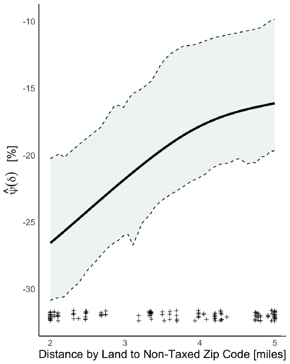
Figure 2: Causal effect curve of the Philadelphia beverage tax through distance to a non-taxed region.

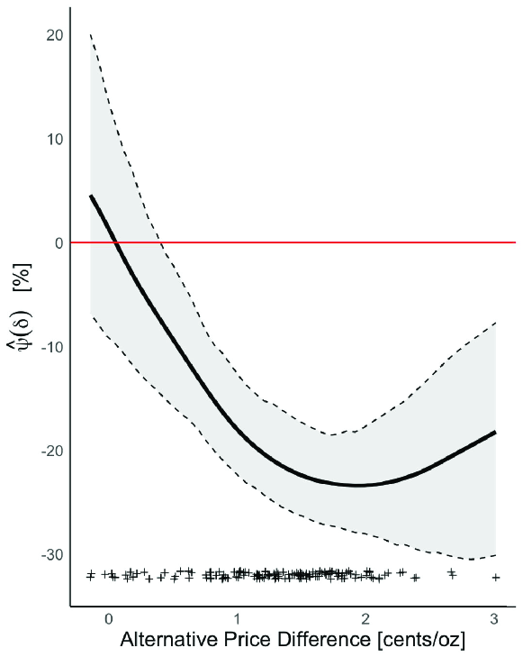
Figure 3: Causal effect curve of the Philadelphia beverage tax through price competition in neighborhood. Here, price competition is measured as the difference between a store price and the minimum alternative among the store’s zip code and adjacent zip codes.

5 Discussion

In this work, we leverage recent DiD methodologies for continuous exposures to develop a robust framework for evaluating the effects of specific policy mechanisms. Our framework, designed to study the Philadelphia beverage tax policy, emphasizes key challenges such as separating multiple mechanisms and accounting for economic competition. In an analysis of the Philadelphia beverage tax policy, we found…

In addition to the methodology inspired by semi-parametric and non-parametric efficiency theory, an important contribution of our work to the literature on policy evaluations is the conceptualization of policy-relevant mechanisms under hypothetical interventions where all units receive a certain exposure level or exposure levels are randomized. While our focus is on the Philadelphia beverage tax, our framework is broadly applicable to other policies – such as the vaccination, gun restriction, and abortion policies – that may involve similarly complex mechanisms like spillover effects or interference.

Still in their formative stages, the methodologies we build upon require strong identification and modeling assumptions. The inclusion of continuous measures of mechanisms, for instance, demands more rigorous counterfactual parallel trends assumptions as well as more complex outcome and generalized propensity score models. Consequently, researchers must carefully consider the sensitivity of estimates to assumption violations and modeling choices, an important area of future development.

There are also numerous directions for expanding this framework to accommodate additional complexities and study objectives. For example, we focused on prices and sales at pharmacies even though many beverages in Philadelphia are sold at supermarkets and cross-over between supermarkets and pharmacies is pharmacy [22]. Such cross-over may be more likely to occur from pharmacies to supermarkets and could be explored by including supermarket prices in the measures of price competition or assessing correlation between supermarket and pharmacy sales.

Additionally, we also did not incorporate sales data from non-taxed stores to avoid making assumptions about the underlying network structure by which Philadelphia consumers travel to nearby non-taxed stores. Attributing sales lost in one region to sales lost in another region is complicated by the incomplete coverage of stores in each region and may make approaches even more sensitive to misspecification. However, the potential for bias due to missing stores also holds true when evaluating price competition. Future work should consider these network structure and missingness patterns if information on travel patterns and the overall population of stores are available.

Lastly, our analysis of price change does not account for the price fluctuations that may occur in the long-term following the tax, driven by changes in sales. We used the initial post-tax price change as a proxy unaffected by post-tax outcomes, but future work could explore these as dynamic treatment regimes to capture the evolving nature of price adjustments.

Acknowledgements

This work was supported by NSF Grant 2149716 (PIs: Mitra and Lee).

References

- \bibcommenthead
- Abadie [\APACyear2005] \APACinsertmetastarAbadie2005SemiparametricEstimators{APACrefauthors}Abadie, A. \APACrefYearMonthDay20051. \BBOQ\APACrefatitleSemiparametric Difference-in-Differences Estimators Semiparametric Difference-in-Differences Estimators.\BBCQ \APACjournalVolNumPagesThe Review of Economic Studies7211–19, {APACrefDOI} https://doi.org/10.1111/0034-6527.00321 \PrintBackRefs\CurrentBib
- Andreyeva \BOthers. [\APACyear2022] \APACinsertmetastarAndreyeva2022OutcomesBeverages{APACrefauthors}Andreyeva, T., Marple, K., Marinello, S., Moore, T.E.\BCBL Powell, L.M. \APACrefYearMonthDay20226. \BBOQ\APACrefatitleOutcomes Following Taxation of Sugar-Sweetened Beverages Outcomes Following Taxation of Sugar-Sweetened Beverages.\BBCQ \APACjournalVolNumPagesJAMA Network Open56e2215276, {APACrefDOI} https://doi.org/10.1001/jamanetworkopen.2022.15276 \PrintBackRefs\CurrentBib
- Angrist \BBA Pischke [\APACyear2008] \APACinsertmetastarAngrist2008MostlyEconometrics{APACrefauthors}Angrist, J.D.\BCBT \BBA Pischke, J\BHBIS. \APACrefYear2008. \APACrefbtitleMostly Harmless Econometrics Mostly Harmless Econometrics. \APACaddressPublisherPrinceton University Press. \PrintBackRefs\CurrentBib
- Aronow \BBA Samii [\APACyear2017] \APACinsertmetastarAronow2013{APACrefauthors}Aronow, P.M.\BCBT \BBA Samii, C. \APACrefYearMonthDay201712. \BBOQ\APACrefatitleEstimating average causal effects under general interference, with application to a social network experiment Estimating average causal effects under general interference, with application to a social network experiment.\BBCQ \APACjournalVolNumPagesThe Annals of Applied Statistics114, {APACrefDOI} https://doi.org/10.1214/16-AOAS1005 \PrintBackRefs\CurrentBib
- Balzer \BBA Westling [\APACyear2023] \APACinsertmetastarBalzer2023InvitedResearch{APACrefauthors}Balzer, L.B.\BCBT \BBA Westling, T. \APACrefYearMonthDay20239. \BBOQ\APACrefatitleInvited Commentary: Demystifying Statistical Inference When Using Machine Learning in Causal Research Invited Commentary: Demystifying Statistical Inference When Using Machine Learning in Causal Research.\BBCQ \APACjournalVolNumPagesAmerican Journal of Epidemiology19291545–1549, {APACrefDOI} https://doi.org/10.1093/aje/kwab200 \PrintBackRefs\CurrentBib
- Callaway \BOthers. [\APACyear2024] \APACinsertmetastarCallaway2024Difference-in-differencesTreatment{APACrefauthors}Callaway, B., Goodman-Bacon, A.\BCBL Sant’Anna, P.H. \APACrefYearMonthDay20242. \APACrefbtitleDifference-in-differences with a Continuous Treatment Difference-in-differences with a Continuous Treatment \APACbVolEdTR\BTR. \APACaddressInstitutionCambridge, MANational Bureau of Economic Research. \PrintBackRefs\CurrentBib
- Dorie \BOthers. [\APACyear2019] \APACinsertmetastarDorie2019AutomatedCompetition{APACrefauthors}Dorie, V., Hill, J., Shalit, U., Scott, M.\BCBL Cervone, D. \APACrefYearMonthDay20192. \BBOQ\APACrefatitleAutomated versus Do-It-Yourself Methods for Causal Inference: Lessons Learned from a Data Analysis Competition Automated versus Do-It-Yourself Methods for Causal Inference: Lessons Learned from a Data Analysis Competition.\BBCQ \APACjournalVolNumPagesStatistical Science341, {APACrefDOI} https://doi.org/10.1214/18-STS667 \PrintBackRefs\CurrentBib
- Efron \BBA Tibshirani [\APACyear1993] \APACinsertmetastarEfronTibshirani1993{APACrefauthors}Efron, B.\BCBT \BBA Tibshirani, R.J. \APACrefYear1993. \APACrefbtitleAn Introduction to the Bootstrap An Introduction to the Bootstrap. \APACaddressPublisherNew York, NYChapman & Hall. \PrintBackRefs\CurrentBib
- Hastie [\APACyear2020] \APACinsertmetastarHastie2020Gam:Models{APACrefauthors}Hastie, T. \APACrefYearMonthDay2020. \APACrefbtitlegam: Generalized Additive Models. gam: Generalized Additive Models. {APACrefURL} https://CRAN.R-project.org/package=gam \PrintBackRefs\CurrentBib
- Hattersley \BBA Mandeville [\APACyear2023] \APACinsertmetastarHattersley2023GlobalTaxes{APACrefauthors}Hattersley, L.\BCBT \BBA Mandeville, K.L. \APACrefYearMonthDay20233. \BBOQ\APACrefatitleGlobal Coverage and Design of Sugar-Sweetened Beverage Taxes Global Coverage and Design of Sugar-Sweetened Beverage Taxes.\BBCQ \APACjournalVolNumPagesJAMA Network Open63e231412, {APACrefDOI} https://doi.org/10.1001/jamanetworkopen.2023.1412 \PrintBackRefs\CurrentBib
- Hejazi \BOthers. [\APACyear2022] \APACinsertmetastarHejazi2022Haldensify:R{APACrefauthors}Hejazi, N.S., van der Laan, M.J.\BCBL Benkeser, D. \APACrefYearMonthDay20229. \BBOQ\APACrefatitlehaldensify: Highly adaptive lasso conditional density estimation in R haldensify: Highly adaptive lasso conditional density estimation in R.\BBCQ \APACjournalVolNumPagesJournal of Open Source Software7774522, {APACrefDOI} https://doi.org/10.21105/joss.04522 \PrintBackRefs\CurrentBib
- Hettinger \BOthers. [\APACyear2024] \APACinsertmetastarHettinger2024MultiplyExposures{APACrefauthors}Hettinger, G., Lee, Y.\BCBL Mitra, N. \APACrefYearMonthDay20241. \BBOQ\APACrefatitleMultiply Robust Difference-in-Differences Estimation of Causal Effect Curves for Continuous Exposures Multiply Robust Difference-in-Differences Estimation of Causal Effect Curves for Continuous Exposures.\BBCQ \PrintBackRefs\CurrentBib
- Hettinger \BOthers. [\APACyear2023] \APACinsertmetastarHettinger2023EstimationTax{APACrefauthors}Hettinger, G., Roberto, C., Lee, Y.\BCBL Mitra, N. \APACrefYearMonthDay20231. \BBOQ\APACrefatitleEstimation of Policy-Relevant Causal Effects in the Presence of Interference with an Application to the Philadelphia Beverage Tax Estimation of Policy-Relevant Causal Effects in the Presence of Interference with an Application to the Philadelphia Beverage Tax.\BBCQ \APACjournalVolNumPagesarXiv, \PrintBackRefs\CurrentBib
- Kennedy [\APACyear2022] \APACinsertmetastarKennedy2022SemiparametricReview{APACrefauthors}Kennedy, E.H. \APACrefYearMonthDay20223. \BBOQ\APACrefatitleSemiparametric doubly robust targeted double machine learning: a review Semiparametric doubly robust targeted double machine learning: a review.\BBCQ \APACjournalVolNumPagesarXiv, \PrintBackRefs\CurrentBib
- Kennedy \BOthers. [\APACyear2017] \APACinsertmetastarKennedy2017NonparametricEffects{APACrefauthors}Kennedy, E.H., Ma, Z., McHugh, M.D.\BCBL Small, D.S. \APACrefYearMonthDay20179. \BBOQ\APACrefatitleNon‐parametric methods for doubly robust estimation of continuous treatment effects Non‐parametric methods for doubly robust estimation of continuous treatment effects.\BBCQ \APACjournalVolNumPagesJournal of the Royal Statistical Society: Series B (Statistical Methodology)7941229–1245, {APACrefDOI} https://doi.org/10.1111/rssb.12212 \PrintBackRefs\CurrentBib
- Lahiri [\APACyear1999] \APACinsertmetastarLahiri1999TheoreticalMethods{APACrefauthors}Lahiri, S.N. \APACrefYearMonthDay19993. \BBOQ\APACrefatitleTheoretical comparisons of block bootstrap methods Theoretical comparisons of block bootstrap methods.\BBCQ \APACjournalVolNumPagesThe Annals of Statistics271, {APACrefDOI} https://doi.org/10.1214/aos/1018031117 \PrintBackRefs\CurrentBib
- Lewis \BOthers. [\APACyear2020] \APACinsertmetastarLewis2020AHealth{APACrefauthors}Lewis, C.C., Boyd, M.R., Walsh-Bailey, C., Lyon, A.R., Beidas, R., Mittman, B.\BDBLChambers, D.A. \APACrefYearMonthDay202012. \BBOQ\APACrefatitleA systematic review of empirical studies examining mechanisms of implementation in health A systematic review of empirical studies examining mechanisms of implementation in health.\BBCQ \APACjournalVolNumPagesImplementation Science15121, {APACrefDOI} https://doi.org/10.1186/s13012-020-00983-3 \PrintBackRefs\CurrentBib
- McCulloch \BOthers. [\APACyear2021] \APACinsertmetastarMcCulloch2021BART:Trees{APACrefauthors}McCulloch, R., Sparapani, R., Spanbauer, C., Gramacy, R.\BCBL Pratola, M. \APACrefYearMonthDay2021. \APACrefbtitleBART: Bayesian Additive Regression Trees. BART: Bayesian Additive Regression Trees. {APACrefURL} https://CRAN.R-project.org/package=BART \PrintBackRefs\CurrentBib
- Muth \BOthers. [\APACyear2016] \APACinsertmetastarMuthIRI2016{APACrefauthors}Muth, M., Sweitzer, M., Brown, D., Capogrossi, K., Karns, S., Levin, D.\BDBLZhen, C. \APACrefYearMonthDay20164. \APACrefbtitleUnderstanding IRI household-based and store-based scanner data. Understanding IRI household-based and store-based scanner data. \PrintBackRefs\CurrentBib
- Naimi \BOthers. [\APACyear2023] \APACinsertmetastarNaimi2023ChallengesAlgorithms{APACrefauthors}Naimi, A.I., Mishler, A.E.\BCBL Kennedy, E.H. \APACrefYearMonthDay20239. \BBOQ\APACrefatitleChallenges in Obtaining Valid Causal Effect Estimates With Machine Learning Algorithms Challenges in Obtaining Valid Causal Effect Estimates With Machine Learning Algorithms.\BBCQ \APACjournalVolNumPagesAmerican Journal of Epidemiology19291536–1544, {APACrefDOI} https://doi.org/10.1093/aje/kwab201 \PrintBackRefs\CurrentBib
- Pollack Porter \BOthers. [\APACyear2018] \APACinsertmetastarPollackPorter2018TheProblems{APACrefauthors}Pollack Porter, K.M., Rutkow, L.\BCBL McGinty, E.E. \APACrefYearMonthDay201811. \BBOQ\APACrefatitleThe Importance of Policy Change for Addressing Public Health Problems The Importance of Policy Change for Addressing Public Health Problems.\BBCQ \APACjournalVolNumPagesPublic Health Reports1331_suppl9S-14S, {APACrefDOI} https://doi.org/10.1177/0033354918788880 \PrintBackRefs\CurrentBib
- Roberto \BOthers. [\APACyear2019] \APACinsertmetastarRoberto2019AssociationSetting{APACrefauthors}Roberto, C.A., Lawman, H.G., LeVasseur, M.T., Mitra, N., Peterhans, A., Herring, B.\BCBL Bleich, S.N. \APACrefYearMonthDay20195. \BBOQ\APACrefatitleAssociation of a Beverage Tax on Sugar-Sweetened and Artificially Sweetened Beverages With Changes in Beverage Prices and Sales at Chain Retailers in a Large Urban Setting Association of a Beverage Tax on Sugar-Sweetened and Artificially Sweetened Beverages With Changes in Beverage Prices and Sales at Chain Retailers in a Large Urban Setting.\BBCQ \APACjournalVolNumPagesJAMA321181799, {APACrefDOI} https://doi.org/10.1001/jama.2019.4249 \PrintBackRefs\CurrentBib
- Sant’Anna \BBA Zhao [\APACyear2020] \APACinsertmetastarSantanna2020{APACrefauthors}Sant’Anna, P.H.\BCBT \BBA Zhao, J. \APACrefYearMonthDay202011. \BBOQ\APACrefatitleDoubly robust difference-in-differences estimators Doubly robust difference-in-differences estimators.\BBCQ \APACjournalVolNumPagesJournal of Econometrics2191101–122, {APACrefDOI} https://doi.org/10.1016/j.jeconom.2020.06.003 \PrintBackRefs\CurrentBib
- The Robert Graham Center [\APACyear2018] \APACinsertmetastarTheRobertGrahamCenter2018SocialSDI{APACrefauthors}The Robert Graham Center \APACrefYearMonthDay201811. \APACrefbtitleSocial deprivation index (SDI). Social deprivation index (SDI). {APACrefURL} https://www.graham-center.org/rgc/maps-data-tools/sdi/social-deprivation-index.html \PrintBackRefs\CurrentBib
- M. van der Laan [\APACyear2017] \APACinsertmetastarvanderLaan2017ALasso{APACrefauthors}van der Laan, M. \APACrefYearMonthDay201711. \BBOQ\APACrefatitleA Generally Efficient Targeted Minimum Loss Based Estimator based on the Highly Adaptive Lasso A Generally Efficient Targeted Minimum Loss Based Estimator based on the Highly Adaptive Lasso.\BBCQ \APACjournalVolNumPagesThe International Journal of Biostatistics132, {APACrefDOI} https://doi.org/10.1515/ijb-2015-0097 \PrintBackRefs\CurrentBib
- M.J. van der Laan \BOthers. [\APACyear2007] \APACinsertmetastarvanderLaan2007SuperLearner{APACrefauthors}van der Laan, M.J., Polley, E.C.\BCBL Hubbard, A.E. \APACrefYearMonthDay20071. \BBOQ\APACrefatitleSuper Learner Super Learner.\BBCQ \APACjournalVolNumPagesStatistical Applications in Genetics and Molecular Biology61, {APACrefDOI} https://doi.org/10.2202/1544-6115.1309 \PrintBackRefs\CurrentBib
- Zeldow \BBA Hatfield [\APACyear2021] \APACinsertmetastarZeldow2021ConfoundingStudies{APACrefauthors}Zeldow, B.\BCBT \BBA Hatfield, L.A. \APACrefYearMonthDay202110. \BBOQ\APACrefatitleConfounding and regression adjustment in difference‐in‐differences studies Confounding and regression adjustment in difference‐in‐differences studies.\BBCQ \APACjournalVolNumPagesHealth Services Research565932–941, {APACrefDOI} https://doi.org/10.1111/1475-6773.13666 \PrintBackRefs\CurrentBib