Thermoelectric Properties of Type-I and Type-II Nodal Line Semimetals: A Comparative Study

Abstract

We investigate the thermoelectric (TE) properties of nodal line semimetals (NLSs) using a combination of semi-analytical calculations within Boltzmann’s linear transport theory and the relaxation time approximation, along with first-principles calculations for the so-called type-I and type-II NLSs. We consider the conduction and valence bands that cross near the Fermi level of these materials through first-principles calculations of typical type-I (TiS) and type-II (Mg₃Bi₂) NLSs and use the two-band model fit to find the Fermi velocity $v_{F}$ and effective mass $m$ that will be employed as the initial energy dispersion parameters. The optimum curvature value for each energy band is searched by tuning the energy dispersion parameters to improve the TE properties of the NLss. We can obtain the best $\sim$$3.5\%$ increase in the Seebeck coefficient peak value compared to those using the initial parameter value in the type-I NLS, with the Seebeck coefficient ranging from $0.509S_{0}$ to $0.527S_{0}$ where $S_{0}\approx 86.17\,\,\upmu\mathrm{V/K}$. Meanwhile, the best increase in power factor, as large as $\sim$$83\%$ the initial value, can be obtained in the type-II NLS when $v_{F}$ is lowered. By systematically comparing all of our calculation results, we observed that tuning $v_{F}$ significantly improves TE properties in both types of NLS compared to tuning $m$. Our work is expected to trigger further calculations to scan other potential TE materials, particularly in the class of semimetals, by manipulating their band structure through the variation of the curvatures of their energy bands.

Keywords: Thermoelectricity, Nodal line semimetals, Two-band model, Boltzmann transport

1 Introduction

Among the primary energy sources such as gas, oil, and coal that are consumed by humans, it has been estimated that only one-third is used effectively, and two-thirds is wasted, most of which are in the form of heat [1, 2, 3, 4]. This form of energy can be converted into useful electrical energy through the so-called thermoelectric (TE) materials. Unfortunately, TE devices often have lower efficiency than most energy conversion schemes. One can assess the TE performance through some parameters such as figures of merit: $ZT=S^{2}\sigma T/\kappa$, where $S$ is the Seebeck coefficient, $\sigma$ is the electrical conductivity, $T$ is the operating temperature, and $\kappa$ is the total thermal conductivity. The thermal conductivity here is a sum of the electronic thermal conductivity ($\kappa_{e}$) and the lattice thermal conductivity ($\kappa_{ph}$), $\kappa=\kappa_{e}+\kappa_{ph}$. The figure of merit is also proportional to the power factor ($\mathrm{PF}$) by the following relation: $ZT=\mathrm{PF}\cdot T/\kappa$, where $\mathrm{PF}=S^{2}\sigma$. From this expression, we can see that a good TE material should possess good electrical conduction and thermal isolation. In other words, one should maximize the Seebeck coefficient and electrical conductivity to obtain a good TE material, while simultaneously, the thermal conductivity should be minimized. Unfortunately, $\sigma$ and $\kappa$ are strongly coupled with each other, hence making it difficult to find the material with high $ZT$ [5, 6, 7, 8, 9, 10, 11, 12, 13]. The interplay among these parameters is primarily governed by the Wiedemann-Franz law, which states that the ratio between $\sigma$ and $\kappa_{e}$ is constant. Therefore, obtaining a material with high $\sigma$ while possessing low thermal conductivity $\kappa$ is very challenging since $\kappa$ also increases when $\sigma$ is enhanced.

Many attempts to decouple the interdependent TE parameters have been proposed to obtain as large $ZT$ as possible for various materials. Some examples of such efforts are carrier concentration optimization [14, 15], nanostructuring materials [16, 17, 18, 19, 20], band convergence engineering [21, 22], and hierarchical architecture consideration [23, 24]. Of various methods used to scan potential TE materials, the band engineering methods such as tuning the gap [25] and the effective mass [26, 27, 28] in terms of the curvature of the band could be effective because these methods use a relatively cheap computational method by considering only the energy dispersion relation $E(k)$ and the scattering lifetime $\uptau(E)$. By doing band-gap tuning or changing the combination of the band structure, one can obtain the optimized structure that will give better TE properties. Several works related to band engineering method have been performed for many types of band structures, such as pudding-mold bands [29, 30, 31, 32, 33], parabolic bands [34, 35, 36], and the linear Dirac bands [37, 38].

Metals and semimetals are usually not considered as good TE materials due to their poor performance originating from the absence of the energy gap which makes the contributions of electrons and holes in the Seebeck coefficient cancel each other. By contrast, the existence of the heavy bands alongside the Dirac bands gives a high PF value in a semimetal like $\mathrm{CoSi}$ [35]. Recently, materials with non-trivial band topology such as the nodal line semimetals (NLSs) [39, 40, 41, 42, 43], in which the conduction and valence bands intersect in the form of a line (called the nodal line), have received some attention due to their unique properties and characteristics. The NLSs can be classified into type-I and type-II NLSs based on the slopes of the bands along their nodal lines. The type-I NLS possesses two bands with oppositely aligned slopes near the nodal line and one of its bands is tilted slightly, while the type-II NLS has bands with the same slope near the nodal line because one of its bands is completely tipped over  [44]. Other works have also shown that some NLS phases found in $\mathrm{Nb}_{3}\mathrm{GeTe_{6}}$ [45] or $\mathrm{YbMnSb}_{2}$ [46] might be promising for TE applications with a Seebeck coefficient twice that of normal metals.

It should be noted that the existence of an intersection between a heavy band and Dirac bands at the Fermi level is found to enhance PF due to the improved electron-phonon scattering in the form of a sharp spike density of states (DOS) [34, 47]. Specifically, the existing heavy band acts as a filter for the low-energy carriers to be excited [48, 49]. This unbalanced condition will lead to the Seebeck coefficient enhancement [50]. However, the effects of specific electronic band properties such as band curvature and slope on TE properties of NLS type-I are yet unknown. Furthermore, we wonder that although the type-II NLS was claimed to be a promising TE material [51], a systematic comparison of TE properties between type-I and type-II NLSs is not available. Regarding this fact, we are fascinated to find out which type of NLSs will have the higher enhancement of TE performance.

In this work, we will discuss the TE properties of type-I (type-II) NLS materials by using $\mathrm{TiS}$ and $\mathrm{Mg}_{3}\mathrm{Bi}_{2}$ as model materials for each type, respectively. We calculate TE properties by employing a two-band model where we consider two energy bands of each NLS, namely conduction and valence bands, near the Fermi level. Then, we will tune the value of energy dispersion parameters from each band which also alters the shape of the band itself, and see its implication on the TE properties of each NLS. As we will see later, it will greatly affect the TE properties of the NLSs. The rest of the paper is organized as follows. In Section 2, we show the model of the band structure that is considered here for both types of NLSs from the energy dispersion and DOS for both bands to the semi-analytical methods used here to obtain TE properties within the constant relaxation time approximation (CRTA). We also show the computational parameters used here to do the first-principles calculations. Section 3 contains our results from the model; it consists of two subsections that discuss the TE properties of type-II and type-II NLSs, respectively. This paper is concluded in Section 4.

2 Model and Methods

In this section, we begin by outlining the band structure model for each type of NLS considering the energy dispersion of each band. Then, we will show how to apply this model to our semianalytical calculations. Lastly, we will briefly outline the computational parameter used in our first-principles calculations.

2.1 Two-band model

The TE properties can be calculated using the Boltzmann transport theory with relaxation time approximation (RTA). In this approach, we express the TE properties (Seebeck coefficient, electrical conductivity, and electron thermal conductivity) in terms of the TE integrals $\mathcal{L}_{i}$ as [52, 38, 45, 46, 53]

$$S=\frac{1}{eT}\frac{\mathcal{L}_{1}}{\mathcal{L}_{0}}$$ (1)

$$\sigma=e^{2}\mathcal{L}_{0},$$ (2)

and

$$\kappa_{e}=\frac{1}{T}\left(\mathcal{L}_{2}-\frac{\mathcal{L}_{1}^{2}}{\mathcal{L}_{0}}\right),$$ (3)

respectively. Where $\mathcal{L}_{i}$ depends on the transport properties of the material according to

$$\mathcal{L}_{i}=\int\uptau v^{2}g(E)\left(-\frac{\partial f}{\partial E}\right)(E-\mu)^{i}dE.$$ (4)

In Eq. (4), $i={0,1,2}$, $\tau$ is the relaxation time, $v=\hbar^{-1}|\gradient_{\mathbf{k}}{E/\sqrt{3}}|$ is the electron longitudinal velocity, $g(E)$ is the density of states (DOS), and $f(E)$ is the Fermi-Dirac distribution:

$$f(E)=\frac{1}{1+\exp[(E-\mu)/k_{B}T]}$$ (5)

with its partial derivative with respect to energy $E$:

$$\frac{\partial f}{\partial E}=-\frac{\exp\left[(E-\mu)/k_{B}T\right]}{(1+\exp[(E-\mu)/k_{B}T])^{2}}\,\left(\frac{1}{k_{B}T}\right)$$ (6)

where $k_{B}$, $\mu$, and $T$ is Boltzmann constant, chemical potential, and temperature, respectively. Eq. (4) is often computed by integration of all bands available over the entire range of energy $E=[-\infty,\infty]$. Nevertheless, for a large number of materials, the thermoelectric characteristics depend mainly on the structure of the electronic bands near the Fermi level [54]. We also need to remember that Eq. (4) is only defined in one band formulation.

Since we consider two bands as the main contributors to the TE properties, we break down Eq. (4) as the sum of conduction and valence band contributions, i.e., [52]

$$\mathcal{L}_{c,i}=\int_{E_{0},c}^{\infty}\tau v^{2}g(E)\left(-\frac{\partial f}{\partial E}\right)(E-\mu)^{i}\,dE,$$ (7)

and

$$\mathcal{L}_{v,i}=\int_{-\infty}^{E_{0,v}}\tau v^{2}g(E)\left(-\frac{\partial f}{\partial E}\right)(E-\mu)^{i}\,dE$$ (8)

where $E_{0,c}$ and $E_{0,v}$ denote the energy at the band edge of the conduction band and of the valence band, respectively. The procedure is justified as we can see from the previous work [55]. Following this division, the TE properties of our material can also be decomposed into conduction and valence band components, (denoted by $c$ and $v$ subscript respectively), such that the total TE transport coefficients are given by

$$S=\frac{S_{c}\sigma_{c}+S_{v}\sigma_{v}}{\sigma_{c}+\sigma_{v}},$$ (9)

$$\sigma=\sigma_{c}+\sigma_{v},$$ (10)

and

$$\kappa_{e}=\frac{\sigma_{c}\sigma_{v}}{\sigma_{c}+\sigma_{v}}(S_{c}-S_{v})^{2}+(\kappa_{e,c}+\kappa_{e,v}).$$ (11)

We will apply Eqs. (7)–(11) to our model of type-I and type-II NLSs.

2.1.1 Type-I NLS

In the type-I NLS, the nodal line is formed when the two bands cross with different slope directions. In this model, we use a Dirac band as the conduction band, and a parabolic band as the valence band. The energy dispersion is given by [56, 57]

$$E_{c}(k)=\hbar v_{F}\mathbf{|k|},$$ (12)

for the conduction band and

$$E_{v}(k)=-\frac{\hbar^{2}\mathbf{|k|^{2}}}{2m}+E_{0}$$ (13)

for the valence band, respectively, where $\mathbf{k}$ is the electron wavevector, $v_{F}$ is the Fermi velocity of the Dirac band, $m$ is the effective mass at the edge of the band, and $E_{0}$ an energy parameter that is used to determine the position of the valence band maximum. We also define $g(E)$ and $v(E)$ for conduction band as:

$$g_{c}(E)=\frac{E^{2}}{\pi^{2}\hbar^{3}v_{F}^{3}},$$ (14)

and

$$v_{c}(E)=\frac{v_{F}}{\sqrt{3}}$$ (15)

respectively, while for the valence band we define it as

$$g_{v}(E)=\frac{m}{\hbar^{2}\pi^{2}}\sqrt{\frac{2m(E-E_{0})}{\hbar^{2}}},$$ (16)

and

$$v_{v}(E)=-\frac{1}{\sqrt{3}}\sqrt{\frac{-2(E-E_{0})}{m}.}$$ (17)

By substituting the above definitions of $g(E)$ and $v(E)$ into Eqs. (7) and (8), we obtain:

$$\begin{split}\mathcal{L}_{c,i}&=\frac{(k_{B}T)^{i+2}}{3\pi^{2}\hbar^{3}v_{F}}\int_{0}^{\infty}\tau(x+\eta)^{2}\,x^{i}\frac{\exp(x)}{(1+\exp(x))^{2}}\,dx,\end{split}$$ (18)

and

$$\begin{split}\mathcal{L}_{v,i}=&\frac{2(k_{B}T)^{i+3/2}\sqrt{2m}}{3\pi^{2}\hbar^{3}}\\ &\times\int_{-\infty}^{\varepsilon_{0}}\tau(-x-\eta+\varepsilon_{0})^{3/2}\,x^{i}\frac{\exp(x)}{(1+\exp(x))^{2}}\,dx.\end{split}$$ (19)

Here, $\mu$ and $E_{0}$ parameters have been normalized with the thermal energy $k_{B}T$ such that $\eta=\mu/k_{B}T$ and $\varepsilon_{0}=E_{0}/k_{B}T$, respectively.

2.1.2 Type-II NLS

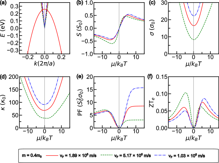
Figure 1: Energy dispersion and TE properties of a model type-I NLS with a varying value of Fermi velocity $v_{F}$. For each combination of the two-band model, we show (a) the energy dispersion, (b) Seebeck coefficient $S$, (c) electrical conductivity $\sigma$, (d) electronic thermal conductivity $\kappa_{e}$, (e) power factor (PF), and (f) electronic figure of merit $ZT_{e}$. TE properties are plotted versus normalized chemical potential $\mu/k_{B}T$. The results for $S$, $\sigma$, and $\kappa_{e}$ are expressed in the units of $S_{0}$, $\sigma_{0}$, and $\kappa_{0}$ respectively.

For a type-II NLS, the crossing between the valence and conduction bands occurs when their slopes have the same direction. We model this using the Dirac band for the conduction band and the Mexican-hat-shaped valence band. The energy dispersion of the valence band is given by [58]:

$$E_{v}(k)=\frac{(\hbar^{2}k^{2}/(4m)-E_{1})^{2}}{E_{1}}+E_{0},$$ (20)

where $E_{1}$ signifies the depth of the central valley of the central valley of the Mexican-hat band measured from the band edge. We define $v(E)$ and $g(E)$ for type-II NLS as:

$$v_{\pm}(\varepsilon)=\sqrt{\frac{k_{B}T(\varepsilon_{0}-\varepsilon)}{3m}}\sqrt{1\pm\sqrt{(\varepsilon_{0}-\varepsilon)/\varepsilon_{1}}}$$ (21)

and

$$g_{\pm}(\varepsilon)=\frac{4m}{\pi^{2}\hbar^{2}}\sqrt{\frac{mk_{B}T\varepsilon_{1}}{\hbar^{2}}}\sqrt{\frac{1\pm\sqrt{(\varepsilon_{0}-\varepsilon)/\varepsilon_{1}}}{(\varepsilon_{0}-\varepsilon)/\varepsilon_{1}}}\>.$$ (22)

Note that since the Mexican-hat band has a valley in the middle of the band, there are two different values for the velocity, one for the outer ring (with a “$+$” sign) and the other for the inner ring (with a “$-$” sign). Substituting Eqs. (21) and (22) into Eq. (8), we obtain the following equations:

$$\begin{split}\mathcal{L}^{out}_{v,i}=&\frac{4(k_{B}T)^{i+3/2}\sqrt{m}}{3\pi^{2}\hbar^{3}}\\ &\times\int_{-\infty}^{\varepsilon_{0}-\eta}\tau\varepsilon_{1}\sqrt{\varepsilon_{0}-x-\eta}\left(1+\sqrt{(\varepsilon_{0}-x-\eta)/\varepsilon_{1}}\right)^{3/2}\\ &\times x^{i}\frac{\exp(x)}{(1+\exp(x))^{2}}\,dx.\\ \end{split}$$ (23)

for the outer ring and

$$\begin{split}\mathcal{L}^{in}_{v,i}=&\frac{4(k_{B}T)^{i+3/2}\sqrt{m}}{3\pi^{2}\hbar^{3}}\\ &\times\int_{\varepsilon_{0}-\varepsilon{1}-\eta}^{\varepsilon_{0}-\eta}\tau\varepsilon_{1}\sqrt{\varepsilon_{0}-x-\eta}\left(1-\sqrt{(\varepsilon_{0}-x-\eta)/\varepsilon_{1}}\right)^{3/2}\\ &\times\frac{\exp(x)}{(1+\exp(x))^{2}}x^{i}\,dx\\ \end{split}$$ (24)

for the inner ring. We also normalize $\mu$, $E_{0}$, and $E_{1}$ parameters with $k_{B}T$ as $\eta=\mu/k_{B}T$, $\varepsilon_{0}=E_{0}/k_{B}T$, and $\varepsilon_{1}=E_{1}/k_{B}T$, respectively.

We express the units of TE properties as $S_{0}$, $\sigma_{0}$, and $\kappa_{0}$. The value of $S_{0}$ is the same for type-I and type-II NLSs, i.e., $S_{0}~{}=~{}k_{B}/e\approx~{}86.17~{}\upmu\mathrm{V/K}$. On the other hand, we distinguish thhe values of $\sigma_{0}$ and $\kappa_{0}$ depending on the NLS types. For the type-I NLS, we have

$$\sigma_{0}=\frac{2\tau e^{2}(k_{B}T)}{3\pi^{2}\hbar^{2}}\,\sqrt{\frac{2mk_{B}T}{\hbar^{2}}}$$ (25)

and

$$\kappa_{0}=\frac{2\tau k_{B}^{3}T^{2}}{3\pi^{2}\hbar^{2}}\,\sqrt{\frac{2mk_{B}T}{\hbar^{2}}},$$ (26)

while for the type-II NLS we have

$$\sigma_{0}=\frac{4\tau e^{2}(k_{B}T)}{3\pi^{2}\hbar^{3}}\,\sqrt{\frac{mk_{B}T}{\hbar^{2}}}$$ (27)

and

$$\kappa_{0}=\frac{4\tau k_{B}^{7/2}T^{5/2}\sqrt{m}}{3\pi^{2}\hbar^{3}}.$$ (28)

2.2 First-principles simulations

We perform first-principles calculations for both types of NLSs by using Quantum ESPREESSO [59] to obtain the electronic properties that will be used to obtain the TE properties and compare them using the model aforementioned above. In this work, the parameters for the TiS and Mg₃Bi₂ as the model materials for the type-I and type-II NLSs, respectively, are obtained from AFLOWLIB database [60]. For the exchange-correlation functional, we employ the generalized gradient approximation (GGA) [61] of the Perdew-Burke-Ernzerhof (PBE) functional. We set the cutoff energy to $300\,\,\mathrm{eV}$, which is already sufficient for the convergence. We also do the calculation to obtain the TE properties of the materials using BoltzTraP2 [62], a package that works based on the Boltzmann transport equation (BTE) to be compared with our model.

The electronic properties from the first-principles calculation can be seen in A. Our results consist of band structures and density of states (DOS). Then, we fit those band structures with the model energy dispersion for each energy band and tune its curvature through varying $v_{F}$ and $m$.

3 Results and discussion

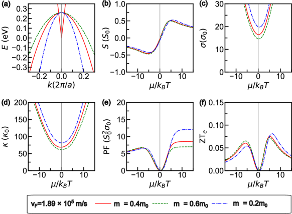
Figure 2: Energy dispersion and TE properties of a model type-I NLS with a varying value of hole effective mass $m$. For each combination of the two-band model, we show (a) the energy dispersion, (b) Seebeck coefficient $S$, (c) electrical conductivity $\sigma$, (d) electronic thermal conductivity $\kappa_{e}$, (e) power factor (PF), and (f) electronic figure of merit $ZT_{e}$. TE properties are plotted versus normalized chemical potential $\mu/k_{B}T$. The results for $S$, $\sigma$, and $\kappa_{e}$ are expressed in the units of $S_{0}$, $\sigma_{0}$, and $\kappa_{0}$ respectively.

Using Eqs. (12)–(13), (18)–(20), and (23)–(24), we will show the schematic plots of the energy dispersion and discuss the TE properties for both type-I and type-II NLSs. The energy dispersion plots are obtained by fitting the energy level coordinates from the first-principles calculations, from their respective reference materials $\mathrm{TiS}$ and $\mathrm{Mg}_{3}\mathrm{Bi}_{2}$ (detailed in A), to our energy dispersion model equations. This allows us to determine the energy dispersion parameters, $v_{F}$ and $m$.

From the fitting, we obtain $v_{F}=1.89\times 10^{5}\,\,\mathrm{m/s}$ and $m=0.4m_{0}$. These values are used in Eqs. (12)–(13) and (20) to plot energy dispersion for each energy band, shown in red in panel (a) of Figs. (1)–(4). To investigate the effects of $v_{F}$ and $m$ on TE properties, we modify the shape of one of the energy bands by selecting higher or lower values of $v_{F}$ and $m$ than those initially obtained. Specifically, we set $v_{F}=5.17\times 10^{5}\,\,\mathrm{m/s}$ and $v_{F}=1.03\times 10^{5}\,\,\mathrm{m/s}$ for the Fermi velocity variation and $m=0.2m_{0}$ and $m=0.8m_{0}$ for the effective mass variation beyond those initial values obtained from the fitting. These altered values are then used in our TE properties calculations, which are carried out numerically using Eqs. (18)–(19) and (23)–(24) through a semi-analytical method with the SciPy package [63] in Python for solving complicated integrals numerically. In all calculations of the TE properties, the temperature is fixed at $T=300\,\,\mathrm{K}$. The calculation codes are available in our GitHub repository [64]. The results for type-I NLS are shown in Figs. 1(a)–(f) and 2(a)–(f), while for type-II NLS are depicted in Figs. 3(a)–(f) and 4(a)–(f). Note that in this work we assess the TE performance of the NLSs in their most optimistic scenario, i.e., when the contribution of $\kappa_{ph}$ to total $\kappa$ is neglected. Therefore, the figure of merit $ZT$ is reduced to the electronic figure of merit $ZT_{e}$ in all of the results discussed in the following sections.

3.1 Type-I NLS

For the type-I NLS, we plot the energy dispersion and TE properties using the parameters mentioned earlier by varying $v_{F}$ and $m$ values in Figs. 1(a)-(f) and 2(a)–(f), respectively. In the following, we plot the TE properties as a function of a dimensionless normalized chemical potential $\mu/k_{B}T$ to observe the doping effect on TE properties by varying the position of chemical potential. A negative $\mu/k_{B}T$ indicates that this is p-type doping where we move the doping level to the valence band, while a positive $\mu/k_{B}T$ indicates n-type doping which means that the doping level is moved to the conduction band. From Eqs. (25) and (26), we obtain the conductivity units of our model type-I NLS as $\sigma_{0}\approx 3.364\times 10^{3}\,\,\mathrm{S/m}$ and $\kappa_{0}\approx 7.494\times 10^{-3}\,\,\mathrm{W/m.k}$

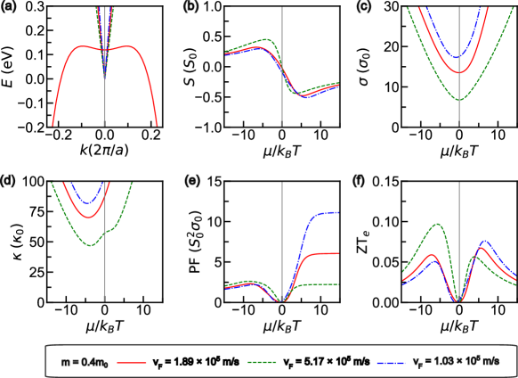
Figure 3: Energy dispersion and TE properties of a model type-II NLS with a varying value of Fermi velocity $v_{F}$. For each combination of the two-band model, we show (a) the energy dispersion, (b) Seebeck coefficient $S$, (c) electrical conductivity $\sigma$, (d) electronic thermal conductivity $\kappa_{e}$, (e) power factor (PF), and (f) electronic figure of merit $ZT_{e}$. TE properties are plotted versus normalized chemical potential $\mu/k_{B}T$. The results for $S$, $\sigma$, and $\kappa_{e}$ are expressed in the units of $S_{0}$, $\sigma_{0}$, and $\kappa_{0}$ respectively.

In Figs. 1(a) and 2(a), we plot energy dispersion relations of each energy band of our type-I NLS model with varying values of $v_{F}$ and $m$, respectively. We observe that in Fig. 1(a) when $v_{F}=1.89\times 10^{5}\mathrm{m/s}$, a tiny increase on the slope of the Dirac band. On the other hand, when $v_{F}=1.03\times 10^{5}$ the Dirac band becomes slightly steeper as shown in blue color in Fig. 1(a). Even though tuning the value of $v_{F}$ only makes a slight change in the slope of the Dirac band, it does however greatly affect all TE properties values as we see in panels (b)–(f) of Fig. 1. Next, in Fig. 2 we see that changing $m$ greatly affects the shape of the parabolic band. When $m=0.2m_{0}$, the parabolic band becomes a light band, while when $m=0.8m_{0}$, the parabolic band becomes a heavy band [55]. Unfortunately, these great changes in the shape of the parabolic band do not affect TE properties compared to $v_{F}$ tuning. In the following part, we will consider how the changes in the shapes of these energy bands affect each of the TE properties.

First, we consider the Seebeck coefficient $S$ for our model type-I NLS in panel (b) of Figs. 1 and 2 with varying $v_{F}$ and $m$ values, respectively. Both figures show an opposite trend in $S$ peak value changes in response to energy dispersion parameters tuning. We also observe a trend where $S$ peak value becomes negative when $\mu/k_{B}T$ is negative. The value is positive when $\mu/k_{B}T$ is shifted to the right where $\mu/k_{B}T$ has positive values. The same trend is also observed in some materials that also have a parabolic band such as $\mathrm{KCaF}_{3}$ [65]. Initially, we set $v_{F}=1.89\times 10^{5}\mathrm{m/s}$ and $m=0.4m_{0}$ in both figures as their initial values which are obtained from fitting. Then, we determine $S$ peak value from both figures using methods that are explained in B. We obtain $S$ peak value of $0.509S_{0}$ for n-type doping and $-0.451S_{0}$ for p-type doping. In Fig. 1(b), there is a pretty significant shift towards $S$ when we tune the initial value of $v_{F}$. When we set $v_{F}=5.17\times 10^{5}\mathrm{m/s}$, the doping level shifts to the right, and $S$ peak value decreases by $\sim$$11\%$ to $0.452S_{0}$ for n-type doping in the left and becomes $-0.598S_{0}$ for the p-type doping. We also notice that the increase in $v_{F}$ greatly affects the $S$ peak value in p-type doping more than in n-type doping. Meanwhile, when $v_{F}=1.03\times 10^{5}\mathrm{m/s}$ the doping level is shifted to the right. The shift is not as further as when $v_{F}=5.17\times 10^{5}\mathrm{m/s}$, but $S$ peak value increases $\sim 7\%$ to $0.545S_{0}$ for n-type doping.

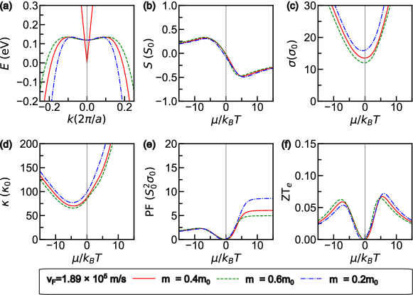
Figure 4: Energy dispersion and TE properties of a model type-II NLS with a varying value of hole effective mass $m$. For each combination of the two-band model, we show (a) the energy dispersion, (b)  Seebeck coefficient $S$, (c) electrical conductivity $\sigma$, (d) electronic thermal conductivity $\kappa_{e}$, (e) power factor (PF), and (f) electronic figure of merit $ZT_{e}$. TE properties are plotted versus normalized chemical potential $\mu/k_{B}T$. The results for $S$, $\sigma$, and $\kappa_{e}$ are expressed in the units of $S_{0}$, $\sigma_{0}$, and $\kappa_{0}$ respectively.

Next, in Fig. 2(b) tuning $m$ value doesn’t have a significant change in $S$ peak value than tuning $v_{F}$. Based on our approximation in Fig. B.2(a), the biggest changes in $S$ occur when $m=0.2m_{0}$ in which the doping level is moved slightly to the left and $S$ peak value increases only by $\sim 3.5\%$ to $0.527S_{0}$ for n-type doping and becomes more negative by $\sim 6\%$ to $-0.421S_{0}$ for p-type doping. On the other hand, the doping level does not appear to be moving towards its initial position when $m$ is increased to $m=0.6m_{0}$ which only results in a minimal change of $S$

Furthermore, we consider the effect of tuning the shape of the energy bands on the magnitude of $\sigma$ and $\kappa$ in panels (c) and (d) of Figs. 1 and 2, respectively. Based on panel (c) from Figs. 1 and 2, we observe that $\sigma$ and $\kappa$ values get greater as the Dirac band gets steeper, i.e. when $v_{F}=1.03\times 10^{5}\mathrm{m/s}$. Meanwhile, for the parabolic band, the increase occurs when the band gets narrower where this is obtained when $m=0.2m_{0}$. In the same way, this is also true for $\mathrm{PF}$ and $ZT_{e}$ as can be seen in panels (e) and (f) of Figs. 1 and 2, respectively. We suspect that this increase results from the term $\frac{(k_{B}T)^{i+2}}{3\pi^{2}\hbar^{3}v_{F}}$ in Eq. (18) and the term $\frac{2(k_{B}T)^{i+3/2}\sqrt{2m}}{3\pi^{2}\hbar^{3}}$ in Eq. (19) for the Dirac band and parabolic band, respectively. This increase also agrees with the Wiedemann-Franz law.

3.2 Type-II NLS

We plot the energy dispersion and TE properties for type-II NLS for by varying the value of $v_{F}$ and $m$ in Figs. 3(a)–(f) and 4(a)–(f), respectively. For TE properties calculation we obtain from Eqs. (27) and (28) $\sigma_{0}\approx 4.757\times 10^{3}\,\,\mathrm{S/m}$ and $\kappa_{0}\approx 5.299\times 10^{-3}\,\,\mathrm{W/m.k}$.

From panel (a) of Figs. 3 and 4, we observe that the given values of $v_{F}$ and $m$ greatly affect the slope of the Dirac band and the depth of the Mexican-hat band NLS type-II. For the Dirac band, it can be seen in Fig. 3(a) that the slope of the Dirac band will increase when $v_{F}=5.17\times 10^{5}\mathrm{m/s}$. On the other hand, when $v_{F}=1.03\times 10^{5}\mathrm{m/s}$, the Dirac band will get steeper and narrower. For the Mexican-hat band in Fig. 4(a), the effect of the value of $m$ on the depth of the Mexican-hat band is as follows. As $m=0.6m_{0}$ , the depth of this band will increase. Contrarily, if $m=0.2m_{0}$, the Mexican-hat band will lose its depth. In the following part, we consider the effects of these energy band adjustments on type-II NLS TE properties.

First, we consider $S$ in panel (b) of Figs. 3 and 4. Initially, from the initial dispersion energy parameters, we obtain the peak value of $S$ of $-0.478S_{0}$ for n-type doping and $0.319S_{0}$ for p-type doping, respectively. In Fig. 3(b), we obtain the highest increase of $S$ peak value about $40\%$ to $\sim$$0.449S_{0}$ when $v_{F}=5.17\times 10^{5}m/s$. This positive value may be attributed to the inclination of the Dirac band. Accordingly, it is better to increase $v_{F}$ since it will also increase carrier mobility because the $S$ is also related to carrier mobility. In contrast, it seems that tuning $m$ doesn’t improve $S$ peak value significantly as seen in Fig. 4(b). The highest increase we obtain only $3.5\%$ to $-0.495S_{0}$ when $m=0.2m_{0}$ for the n-type doping and $7.18\%$ to $0.328S_{0}$ when $m=0.6m_{0}$ for the p-type doping. Therefore, we believe that tuning the shape of the Mexican-hat band through $m$ tuning is not a good idea to improve the TE properties of our type-II NLS model.

Next, in panels (c) and (d) of Fig. 3 we can see that tuning $v_{F}$ and $m$ also cause changes in $\kappa$ and $\sigma$. Even though the increase is not as drastic as in the type-I NLS model, it still greatly affects PF and $\mathrm{ZT_{e}}$ as we explain in the later part. This increase is caused by the term $\frac{(k_{B}T)^{i+2}}{3\pi^{2}\hbar^{3}v_{F}}$, $\frac{4\tau(k_{B}T)^{i+3/2}\sqrt{m}}{3\pi^{2}\hbar^{3}}$, and $\frac{4\tau(k_{B}T)^{i+3/2}\sqrt{m}}{3\pi^{2}\hbar^{3}}$ in Eqs. (18), (24), and (23), respectively.

Furthermore, in panel (e) of Figs. 3 and 4. From the initial energy dispersion parameters, we obtain the respective PF of $6.055S_{0}^{2}\sigma_{0}$ for n-type doping and $2.312S_{0}^{2}\sigma_{0}$ for p-type doping. The increase of PF peak value that occurs in Fig. 3(e) is about $83\%$ larger than the initial value when $v_{F}=1.03\times 10^{5}\mathrm{m/s}$ which changes PF peak value to $\sim$$11.085S^{2}_{0}\sigma_{0}$ for n-type doping. We also observe changes in PF peak value caused by $m$ tuning, although not as large as when we tune the $v_{F}$. We obtain a PF peak value increase of $41.29\%$ to $8.555S_{0}^{2}\sigma_{0}$ when $m=0.2m_{0}$, while for the p-type doping the increase we obtain is not significant. We observe that those increases in PF might be caused by a simultaneous increase in $\sigma$ in panel (c) of Figs. 3 and 4 through the relation $\mathrm{PF}=S^{2}\sigma$. Therefore, we suggest that tuning $v_{F}$ is the best option to obtain the optimum value for PF.

Finally, in panel (f) of Figs. 3 and 4. We obtain the respective $ZT_{e}$ peak values of $0.067$ for n-type doping and $0,059$ p-type doping by using initial energy dispersion parameters, respectively. From Fig. 3(f), we obtain the highest increase in peak value of $ZT_{e}$ for the p-type doping when $v_{F}=5.17\times 10^{5}$. We obtain $28.81\%$ increases in peak value of $ZT_{e}$ $\sim$$0.097$. On the other hand, we obtain $ZT_{e}$ peak value of $\sim 0.076$ when $v_{F}=1.03\times 10^{5}\mathrm{m/s}$ for the n-type doping, which means it only increases $\sim 13.42\%$ from the initial peak value for the n-type doping.

4 Conclusions

We have compared TE properties of NLS type-I and type-II through consideration of energy dispersion shapes by tuning each NLS type curvature. We found that changing the shape of the energy dispersion through making slight changes to its parameters, $v_{F}$ and $m$, can drastically affect the TE properties of both types of NLSs. In particular, the most significant enhancement is in the PF of type-II NLS which can be increased up to $83\%$ from the initial value. By comparing the results of the TE properties calculation with varying $v_{F}$ and $m$ values for both types of NLS, we also found that tuning $v_{F}$ of the linear band provides more significant changes in the TE properties compared to $m$ of either parabolic or Mexican-hat band.

Appendix A Electronic properties of TiS and Mg₃Bi₂ from first-principles simulations

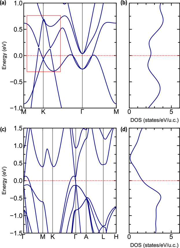
Figure A.1: Electronic properties of our NLS reference materials. Panels (a) and (c) show the results for band structure, while panels (b) and (d) show the results for DOS. The results in panels (a) and (b) are for $\mathrm{TiS}$, and the results in panels (c) and (d) are for $\mathrm{Mg}_{3}\mathrm{Bi}_{2}$.

As mentioned before, we use $\mathrm{TiS}$ and $\mathrm{Mg}_{3}\mathrm{Bi}_{2}$ as our reference materials for type-I and type-II NLS, respectively. Here, we show each of its electronic properties.

In Figs. A.1(a)–(b), we show the electronic properties of $\mathrm{TiS}$. From Fig. A.1(a), we see a band crossing in $\mathrm{M}-\mathrm{K}-\Gamma$ path that confirms that the material belongs to type-I NLS. This also confirms the observation in Ref. [66]. Then, we took the energy band’s energy level coordinates to fit it with our model energy dispersion equation and tune its curvature.

Next, for $\mathrm{Mg}_{3}\mathrm{Bi}_{2}$, we show the electronic properties in Figs. A.1(c)–(d). From Fig. A.1, we can see that there is a crossing in $\mathrm{K}-\Gamma-\mathrm{M}$ which confirms that the material is a type-II NLS. This also confirms some observations done in Ref. [44]. Then, we do the same things mentioned before to fit it with our model energy energy dispersion equations.

Appendix B Peak value approximations for the TE properties

We examine our TE properties calculation results here by approximating its peak value to observe the change in TE properties’ peak value with respect to energy dispersion parameters ($m$ and $v_{F}$). We make our approximations by numerically interpolating the data of TE properties calculation results using the NumPy package.

In Figs. B.1 and B.2, we approximate TE properties peak value in model type-I NLS with varying $v_{F}$ and $m$, respectively. From Fig. B.2(a), a change occurs when $m=0.2m_{0}$ in which the doping level is shifted to the left and $S$ peak value increases only by $\sim 3.5\%$ to $0.527S_{0}$ for n-type doping and becomes more negative by $\sim 6\%$ to $-0.421S_{0}$ for p-type doping. Then, when $m=0.6m_{0}$, the doping level does not appear to be moving towards its initial doping level even though there is a tiny decrease of $\sim$$3.7\%$ in $S$ peak value to $0.490S_{0}$ for n-type doping. Finally, in Figs. B.3 and B.4, we determine TE properties peak value in model type-II NLS with varying $v_{F}$ and $m$, respectively.

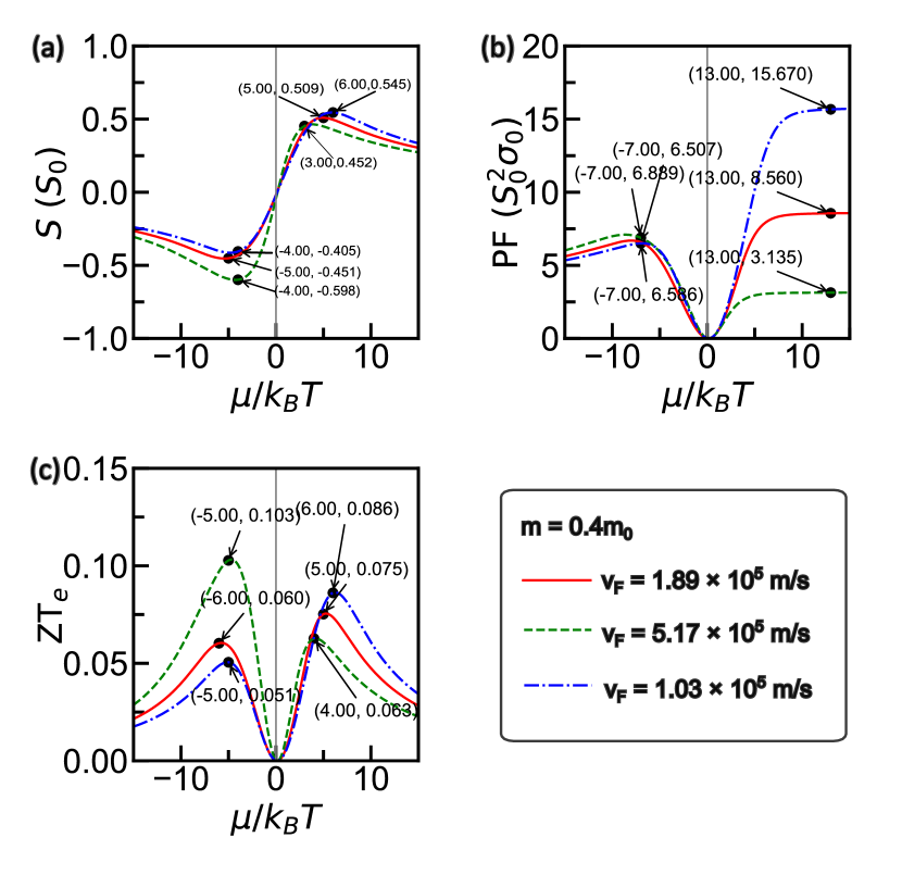
Figure B.1: TE properties peak value approximation for model type-I NLS with varying value of Fermi velocity $v_{F}$. We show the approximate peak values for (a) Seebeck coefficient $S$, (b) power factor (PF), and (c) electronic figure of merit $ZT_{e}$.

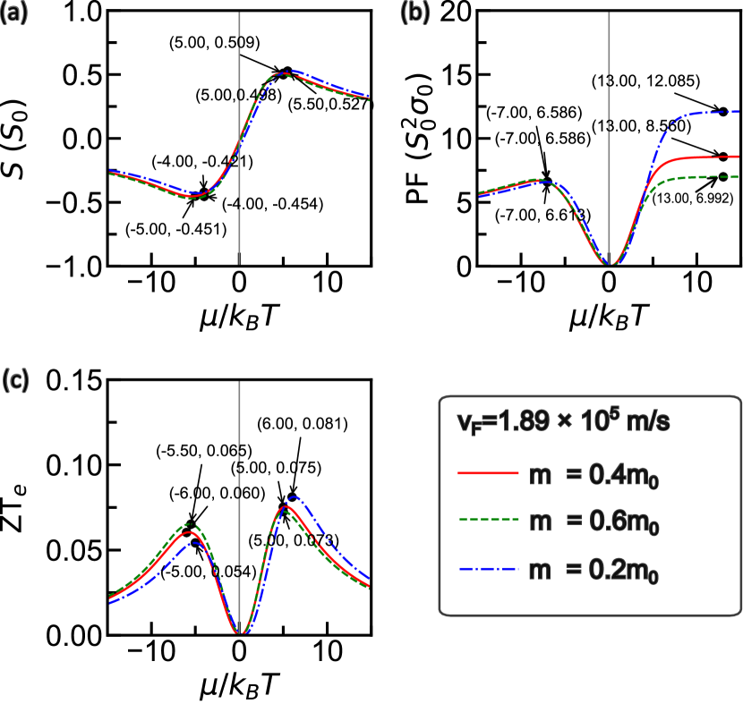
Figure B.2: TE properties peak value approximation for model type-I NLS with varying hole effective mass $m$ values. We show the approximate peak values for (a) Seebeck coefficient $S$, (b) power factor (PF), and (c) electronic figure of merit $ZT_{e}$.

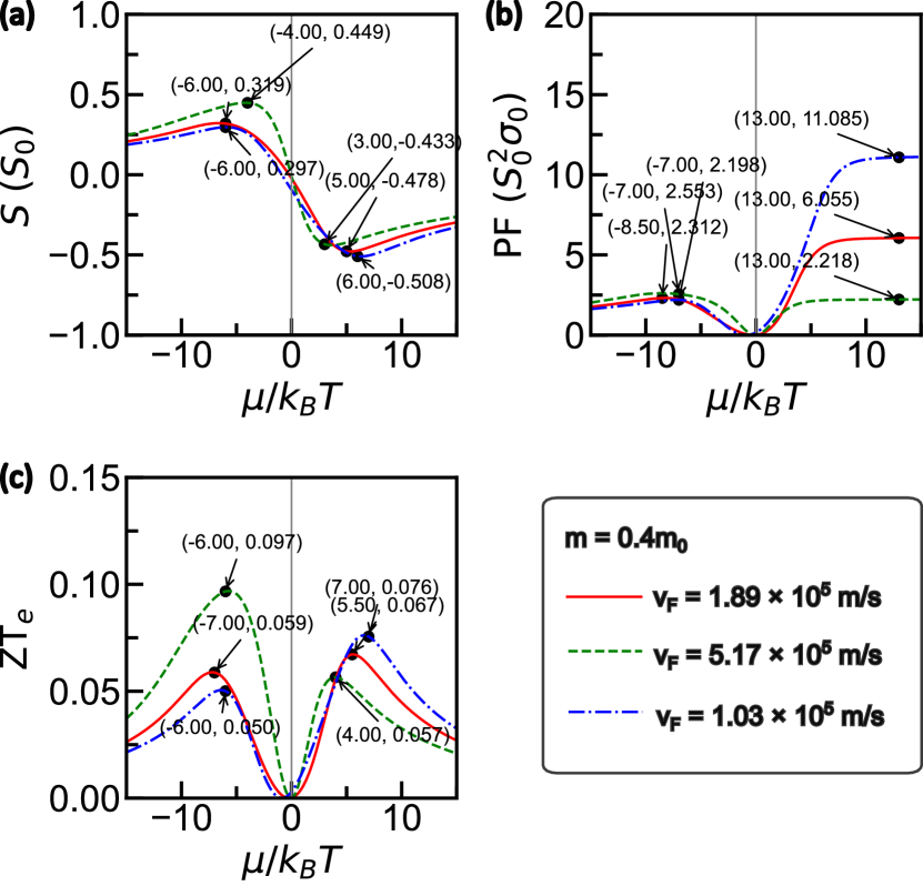
Figure B.3: TE properties peak value approximation for model type-II NLS with varying value of Fermi velocity $v_{F}$. We show the approximate peak values for (a) Seebeck coefficient $S$, (b) power factor (PF), and (c) electronic figure of merit $ZT_{e}$.

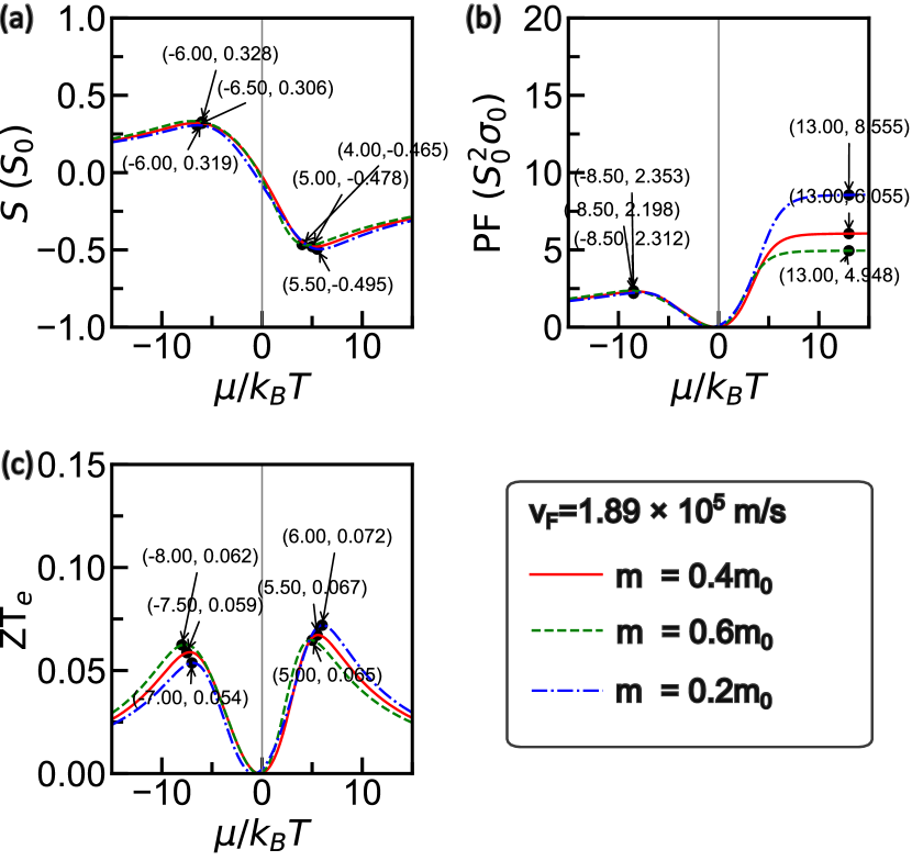
Figure B.4: TE properties peak value approximation for model type-II NLS with varying hole effective mass $m$ values. We show the approximate peak values for (a) Seebeck coefficient $S$, (b) power factor (PF), and (c) electronic figure of merit $ZT_{e}$.

References

References

- [1] Fitriani, Ovik R, Long B, Barma M, Riaz M, Sabri M, Said S and Saidur R 2016 Renew. Sustain. Energy Rev. 64 635–659
- [2] Koumoto K and Mori T 2013 Thermoelectric nanomaterials (Berlin, Heidelberg: Springer)
- [3] Elsheikh M H, Shnawah D A, Sabri M F M, Said S B M, Hassan M H, Bashir M B A and Mohamad M 2014 Renew. Sustain. Energy Rev. 30 337–355
- [4] Zheng X, Liu C, Yan Y and Wang Q 2014 Renew. Sustain. Energy Rev. 32 486–503
- [5] Zeier W G, Zevalkink A, Gibbs Z M, Hautier G, Kanatzidis M G and Snyder G J 2016 Angew. Chem. 55 6826–6841
- [6] Yang J, Xi L, Qiu W, Wu L, Shi X, Chen L, Yang J, Zhang W, Uher C and Singh D J 2016 npj Comput. Mater. 2 1–17
- [7] Jain A, Shin Y and Persson K A 2016 Nat. Rev. Mater. 1 1–13
- [8] Zhu T, Liu Y, Fu C, Heremans J P, Snyder J G and Zhao X 2017 Adv. Mater. 29 1605884
- [9] He J and Tritt T M 2017 Science 357 eaak9997
- [10] Gorai P, Stevanović V and Toberer E S 2017 Nat. Rev, Mater. 2 1–16
- [11] Mao J, Liu Z, Zhou J, Zhu H, Zhang Q, Chen G and Ren Z 2018 Adv. Phys 67 69–147
- [12] Darmawan A, Suprayoga E, AlShaikhi A A and Nugraha A R 2022 Mater. Today Commun 33 104596
- [13] Hu J, Tang Z, Liu J, Liu X, Zhu Y, Graf D, Myhro K, Tran S, Lau C N, Wei J et al. 2016 Phys. Rev. Lett. 117 016602
- [14] Chen Z G, Han G, Yang L, Cheng L and Zou J 2012 Prog. Nat. Sci.: Mater. Int. 22 535–549
- [15] Zhou M, Gibbs Z M, Wang H, Han Y, Li L and Snyder G J 2016 Appl. Phys. Lett. 109 042102
- [16] Poudel B, Hao Q, Ma Y, Lan Y, Minnich A, Yu B, Yan X, Wang D, Muto A, Vashaee D et al. 2008 science 320 634–638
- [17] Ma Y, Hao Q, Poudel B, Lan Y, Yu B, Wang D, Chen G and Ren Z 2008 Nano Lett. 8 2580–2584
- [18] Xie W, Tang X, Yan Y, Zhang Q and Tritt T M 2009 Appl. Phys. Lett. 94
- [19] Xie W, He J, Kang H J, Tang X, Zhu S, Laver M, Wang S, Copley J R, Brown C M, Zhang Q et al. 2010 Nano Lett. 10 3283–3289
- [20] Yan X, Liu W, Chen S, Wang H, Zhang Q, Chen G and Ren Z 2013 Adv. Energy Mater. 3 1195–1200
- [21] Mahan G and Sofo J 1996 Proc. Natl. Acad. Sci. U.S.A. 93 7436–7439
- [22] Mao J, Wang Y, Kim H S, Liu Z, Saparamadu U, Tian F, Dahal K, Sun J, Chen S, Liu W et al. 2015 Nano Energy 17 279–289
- [23] Biswas K, He J, Blum I D, Wu C I, Hogan T P, Seidman D N, Dravid V P and Kanatzidis M G 2012 Nature 489 414–418
- [24] Ren G K, Wang S Y, Zhu Y C, Ventura K J, Tan X, Xu W, Lin Y H, Yang J and Nan C W 2017 Energy Environ. Sci. 10 1590–1599
- [25] Pei Y, Heinz N A and Snyder G J 2011 J. Mater. Chem. 21 18256–18260
- [26] Bilc D, Mahanti S, Quarez E, Hsu K F, Pcionek R and Kanatzidis M 2004 Phys. Rev. Lett. 93 146403
- [27] Heremans J P, Wiendlocha B and Chamoire A M 2012 Energy Environ. Sci. 5 5510–5530 ISSN 1754-5692
- [28] Pei Y, LaLonde A D, Wang H and Snyder G J 2012 Energy Environ. Sci. 5 7963–7969
- [29] Usui H and Kuroki K 2017 J. Appl. Phys 121
- [30] Usui H, Suzuki K, Kuroki K, Nakano S, Kudo K and Nohara M 2013 Phys. Rev. B 88 075140
- [31] Kuroki K and Arita R 2007 J. Phys. Soc. Jpn. 76 083707–083707
- [32] Isaacs E B and Wolverton C 2019 Phys. Rev. Mater 3 015403
- [33] Wei S, Wang C, Fan S and Gao G 2020 J. Appl. Phys 127
- [34] Xia Y, Park J, Ozoliņš V and Wolverton C 2019 Phys. Rev. B 100 201401
- [35] Xia Y, Park J, Zhou F and Ozoliņš V 2019 Phys. Rev. Appl. 11 024017
- [36] Adhidewata J M, Nugraha A R, Hasdeo E H, Estellé P and Gunara B E 2022 Mater. Today Commun. 31 103737
- [37] Adhidewata J M, Nugraha A R, Hasdeo E H and Gunara B E 2022 Indones. J. Appl. Phys. 33 51–57
- [38] Hasdeo E H, Krisna L P A, Hanna M Y, Gunara B E, Hung N T and Nugraha A R T 2019 J. Appl. Phys 126 035109 ISSN 0021-8979
- [39] Shao Y, Rudenko A N, Hu J, Sun Z, Zhu Y, Moon S, Millis A J, Yuan S, Lichtenstein A I, Smirnov D, Mao Z Q, Katsnelson M I and Basov D N 2020 Nat. Phys. 16 636–641 ISSN 1745-2481
- [40] Rudenko A, Stepanov E, Lichtenstein A and Katsnelson M 2018 Phys. Rev. Lett. 120 216401
- [41] Singha R, Pariari A K, Satpati B and Mandal P 2017 Proc. Natl. Acad. Sci. U.S.A. 114 2468–2473
- [42] Ali M N, Schoop L M, Garg C, Lippmann J M, Lara E, Lotsch B and Parkin S S 2016 Sci. Adv. 2 e1601742
- [43] Guan S, Yu Z M, Liu Y, Liu G B, Dong L, Lu Y, Yao Y and Yang S A 2017 npj Quantum Mater. 2 23 ISSN 2397-4648 URL https://doi.org/10.1038/s41535-017-0026-7
- [44] Zhang X, Jin L, Dai X and Liu G 2017 J. Phys. Chem. Lett. 8 4814–4819
- [45] Wang X, Ding G, Khandy S A, Cheng Z, Zhang G, Wang X L and Chen H 2020 Nanoscale 12 16910–16916
- [46] Pan Y, Fan F R, Hong X, He B, Le C, Schnelle W, He Y, Imasato K, Borrmann H, Hess C et al. 2021 Adv. Energy Mater. 33 2003168
- [47] Rudderham C and Maassen J 2021 Phys. Rev. B 103 165406
- [48] Bahk J H and Shakouri A 2016 Phys. Rev. B 93 165209
- [49] Androulakis J, Todorov I, Chung D Y, Ballikaya S, Wang G, Uher C and Kanatzidis M 2010 Phys. Rev. B 82 115209
- [50] Gayner C, Sharma R, Das M K and Kar K K 2016 J. Appl. Phys 120
- [51] Hung N T, Adhidewata J M, Nugraha A R and Saito R 2022 Phys. Rev. B 105 115142
- [52] Goldsmid H J et al. 2010 Introduction to thermoelectricity vol 121 (Springer)
- [53] Ashcroft N W 1976 Saunders College, Philadelphia 120
- [54] Markov M, Hu X, Liu H C, Liu N, Poon S J, Esfarjani K and Zebarjadi M 2018 Sci. Rep. 8 9876
- [55] Chasapis T C, Lee Y, Hatzikraniotis E, Paraskevopoulos K M, Chi H, Uher C and Kanatzidis M G 2015 Phys. Rev. B 91 085207
- [56] Neto A C, Guinea F, Peres N M, Novoselov K S and Geim A K 2009 Rev. Mod. Phys. 81 109
- [57] Ariel V 2012 arXiv preprint arXiv:1207.4282
- [58] Wickramaratne D, Zahid F and Lake R K 2015 J. Appl. Phys 118
- [59] Giannozzi P, Baroni S, Bonini N, Calandra M, Car R, Cavazzoni C, Ceresoli D, Chiarotti G L, Cococcioni M, Dabo I et al. 2009 J. Phys. Condens. Matter 21 395502
- [60] Curtarolo S, Setyawan W, Wang S, Xue J, Yang K, Taylor R H, Nelson L J, Hart G L, Sanvito S, Buongiorno-Nardelli M et al. 2012 Comput. Mater. Sci. 58 227–235
- [61] Perdew J P, Chevary J A, Vosko S H, Jackson K A, Pederson M R, Singh D J and Fiolhais C 1992 Phys. Rev. B 46 6671
- [62] Madsen G K, Carrete J and Verstraete M J 2018 Comput. Phys. Commun. 231 140–145
- [63] Virtanen P, Gommers R, Oliphant T E, Haberland M, Reddy T, Cournapeau D, Burovski E, Peterson P, Weckesser W, Bright J et al. 2020 Nat. Methods 17 261–272
- [64] Python codes to obtain all calculation results from this paper available at https://github.com/Normanthen/NLS-Thermoelectrics
- [65] Ali A, Rahman A U and Rahman G 2019 Phys. B: Condens. Matter 565 18–24
- [66] Xu L, Zhang X, Meng W, He T, Liu Y, Dai X, Zhang Y and Liu G 2020 Journal of Materials Chemistry C 8 14109–14116