Dynamics of switching processes: general results and applications to intermittent active motion

Ion Santraa‡, Kristian Stølevik Olsenb, Deepak Guptac,d‡

Abstract:  Systems switching between different dynamical phases is an ubiquitous phenomenon. The general understanding of such a process is limited. To this end, we present a general expression that captures fluctuations of a system exhibiting a switching mechanism. Specifically, we obtain an exact expression of the Laplace-transformed characteristic function of the particle’s position. Then, the characteristic function is used to compute the effective diffusion coefficient of a system performing intermittent dynamics. Further, we employ two examples: 1) Generalized run-and-tumble active particle, and 2) an active particle switching its dynamics between generalized active run-and-tumble motion and passive Brownian motion. In each case, explicit computations of the spatial cumulants are presented. Our findings reveal that the particle’s position probability density function exhibit rich behaviours due to intermittent activity. Numerical simulations confirm our findings.

1 Introduction

Switching between different dynamical phases is a widespread phenomenon in a wide range of complex systems ^{1, 2}. Many examples can be found in a biological setting, including transitions between stages of the cell-cycle ^{3, 4}, changes in animal motility patterns ^{5, 6}, diffusion of particles in mammalian cells ^{7, 8}, and target-binding proteins that switch between sliding motion along DNA strands and three–dimensional excursions ^{9, 10}.

Living or active systems are ideal candidates for displaying dynamical switching ^{11, 12, 13, 14}. For example, such systems are often capable of processing environmental information, leading to subsequent adaptation and changes in motility patterns ^{15, 16, 17}, a property not shared with their passive counterparts. The study of physical properties of life-like systems often falls under the umbrella of active matter ^{18, 19, 20, 21}. A plethora of examples can be found, ranging from motile cells ²² and synthetic active colloids ²³ on the microscale all the way to macro-scale living organisms ²⁴ and granular systems ^{25, 26, 27}. Several theoretical investigations of active particles that undergo dynamical switching has been seen recently, including switching chirality ^{28, 29, 30, 31} and particles that switch between many possible self-propulsion states  ^{32, 33, 34}. Further, recent theoretical investigations show how such intermittent active phases can aid in spatial exploration and target search ^{35, 16}.

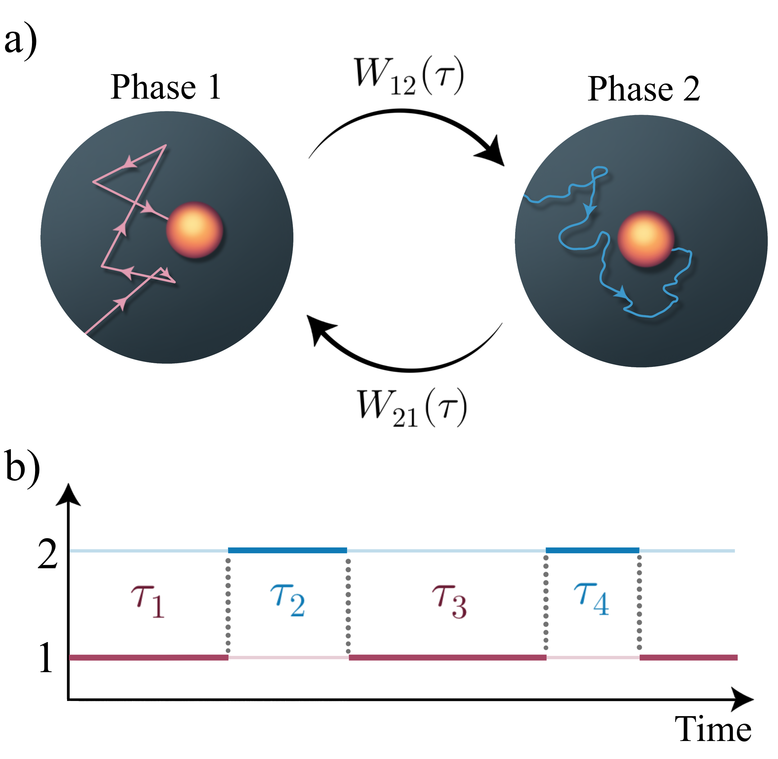
Fig.  1: a) Schematic representation of a two state stochastic process, where a particle iteratively switched between two arbitrary abstract dynamical phases. b) The particle switches between phase 1 and 2 iteratively, with corresponding waiting-times $\tau$, where $\tau$ is chosen from the probability density functions $W_{1\to 2}(\tau)\equiv W_{12}(\tau)$ and $W_{2\to 1}(\tau)\equiv W_{21}(\tau)$.

A widespread type of switching found both on microscopic and macroscopic scales is activity that only acts intermittently, where directed motion is interspersed with passive or immobile phases ^{36, 37, 38, 39, 40, 41, 42, 43, 44, 45, 46, 47, 48, 49, 50, 51, 52, 53}. Interestingly, from an experimental perspective, intermittent activity can easily be achieved in systems of light-activated particles ⁵⁴. Such experimental modelling of active behaviours has opened a door to design self-propelled particles with a broad range of novel behaviours ^{55, 56}, including the ability to make particles reverse their direction of motion with a specified asymmetry in the forward and backward speeds ⁵⁷.

Motivated by the experiment based on light-activated particles ⁵⁴, we present a general framework that captures the dynamics of a two-phase switching process (see Fig. 1). Here, we derive an exact expression for the (Fourier-Laplace transformed) probability density function of an observable that evolves according to the rules of two different phases. We employ the (Fourier-Laplace transformed) probability density function to compute the expression for the effective diffusion of the switching process. Then, we explore two examples of switching processes [1) the generalized run-and-tumble particle and 2) a switching process composed of the generalized run-and-tumble motion and Brownian motion] to investigate their time-dependent properties.

The rest of the paper is organised as follows. Section 2 builds the general framework of the switching process and discusses the method to compute the fluctuations of the particle’s position. Section 3 contains the derivation of the effective diffusion constant for a general scenario. In Sec. 4, we discuss two examples of switching processes, with detailed analysis of their time-dependent properties. Then, we discuss the position probability density function for a generalized run-and-tumble particle switching its behaviour to Brownian motion intermittently in Sec. 5. Finally, we summarize the paper in Sec. 6. Some of the detailed expressions are relegated to Appendices.

2 General formalism

In the past several decades, the theoretical statistical physics community has explored the fascinating nature of dynamical switching processes by investigating its statistical properties. Examples include modelling of dynamical coexistence of slow- and fast-diffusion in liquids and caging effects in glassy materials ^{58, 59}, as well as theoretical work on the dynamical disorder ^{60, 61, 62}. Additionally, stochastic resetting  ^{63, 64, 65, 66, 67, 68, 69, 70}, diffusive systems with a switching diffusion coefficient ^{71, 72, 73, 74, 75}, and alternating ballistic and diffusive phases ^{76, 77, 78, 79} fall under the umbrella of the stochastic switching process. Several frameworks have been proposed to deal with systems exhibiting dynamical switching, such as hybrid and composite stochastic processes ^{80, 71, 81}, piece-wise deterministic Markov processes ⁸² and hidden Markov models ^{83, 84, 85}. Here, we consider a general approach to model systems with switching mechanisms, which enable us to reproduce many of the above examples.

In this paper, we consider a general dynamical process, where a system (henceforth a particle) switches stochastically between two phases, 1 and 2 (Fig. 1). Stochastic dynamics characterize the evolution of this switching mechanism ⁸⁶. Without loss of generality, we assume that the particle’s trajectory begins in the phase 1 and remains in this phase for a time-interval $\tau_{1}$ before switching its phase to phase 2. It executes the phase 2 dynamics for a time-interval $\tau_{2}$, and then, its phase switches back to phase 1. This process iterates until the observation time $t=\sum_{j=1}\tau_{j}$. The waiting time-intervals $\tau_{1},\tau_{3},\dotsc$ ($\tau_{2},\tau_{4},\dotsc$), that correspond to a switch from phase 1 to phase 2 (phase 2 to phase 1), are drawn from the probability density function $W_{12}(\tau)\equiv W_{1\to 2}$ ($W_{21}(\tau)\equiv W_{2\to 1}$), see Fig. 1. Then, the survival probabilities $S_{1}(t)$ or $S_{2}(t)$, respectively, denote the probability that the particle starting from phase 1 or phase 2 has not switched to its complementary phase until time $t$. Mathematically, these read as

$$S_{1}(t)\equiv\int_{t}^{\infty}{\rm d}\tau\leavevmode\nobreak\ W_{12}(\tau)\ ,$$ (1a)

$$S_{2}(t)\equiv\int_{t}^{\infty}{\rm d}\tau\leavevmode\nobreak\ W_{21}(\tau)\ .$$ (1b)

To proceed further, we write the propagator of the particle (probability density function of particle’s position) evolving solely in phase 1 (or phase 2) until time $t$, having started from position $x_{0}$ at time $t_{0}$; this is denoted by $P_{\rm 1}(x,t|x_{0},t_{0})$ [or $P_{\rm 2}(x,t|x_{0},t_{0})$]. Further, we assume no potential energy landscapes in either of these phases; therefore, the particle’s dynamics in each phase depends on the distance covered from its initial location in time $t-t_{0}$. Thus, we write

$$P_{j}(x-x_{0},t-t_{0})\equiv P_{j}(x-x_{0},t-t_{0}|0,0)=P_{j}(x,t|x_{0},t_{0})\ ,$$ (2)

for the phase index $j=\{{\rm 1,2}\}$.

For simplicity of notation, we assume that the particle starts from the origin ($x=0$) at time $t=0$ in phase 1. Let the time-interval between the $i$’th and the $(i+1)$’th switching event be $\tau_{i+1}$, and the displacement in that time-interval be $x_{i+1}$. Then, the propagator accounts the contributions arising from trajectories experiencing different number of switching events until time $t$.

Let us first compute the contribution to the probability density function of the particle’s position $x$ in time $t$, from a trajectory that has not experienced a single switching event until time $t$. This is given by

$$\phi_{0}(x,t)\equiv S_{1}(t)\leavevmode\nobreak\ P_{1}(x,t)\ .$$ (3)

Note that, the right-hand side of the above equation (3) is in a product form. This is because the switching between the phases and the individual dynamics in each phase are independent events.

Now, suppose a single switching event occurs from phase 1 to 2 in time-interval $\tau_{1}$, and in the remaining time $\tau_{2}=t-\tau_{1}$, there is no switching occurs. Then, we have

$$\phi_{1}(x,t) \equiv\int_{-\infty}^{\infty}\leavevmode\nobreak\ {\rm d}x_{1}\int_{-\infty}^{\infty}\leavevmode\nobreak\ {\rm d}x_{2}\leavevmode\nobreak\ \int_{0}^{t}{\rm d}\tau_{1}\leavevmode\nobreak\ W_{12}(\tau_{1})\leavevmode\nobreak\ P_{1}(x_{1},\tau_{1})$$

$$\times\int_{0}^{t}{\rm d}\tau_{2}\leavevmode\nobreak\ S_{2}(\tau_{2})\leavevmode\nobreak\ P_{2}(x_{2},\tau_{2})\delta(x-x_{1}-x_{2})\delta(t-\tau_{1}-\tau_{2})\ .$$ (4)

Several comments are in order. The first part, i.e., $W_{12}(\tau_{1})P_{1}(x_{1},\tau_{1})$, indicates that the particle is evolved by the phase 1 dynamics for a time-interval $\tau_{1}$, and then, underwent a switching event. Further, the second part, i.e., $S_{2}(\tau_{2})P_{2}(x_{2},\tau_{2})$, is for the particle that followed the phase 2 dynamics and did not undergo further switching events in the remaining time-interval $\tau_{2}$. The intervals $\tau_{1}$ and $\tau_{2}$ are arbitrary and hence they have to be integrated over along with a delta function ensuring that the total observation time is $t=\tau_{1}+\tau_{2}$. Another delta function ensures that the particle reaches $x$ after travelling $x_{1}$ and $x_{2}$, respectively, in phase 1 and 2.

The upper limits of the $\tau_{i}$ integrals can be set to $+\infty$, since the delta-function still ensures that the region of integration in the $(\tau_{1},\tau_{2})$ plane remains the same. Then, we have

$$\phi_{1}(x,t) \equiv\int_{-\infty}^{\infty}{\rm d}x_{1}\leavevmode\nobreak\ \int_{-\infty}^{\infty}\leavevmode\nobreak\ {\rm d}x_{2}\leavevmode\nobreak\ \int_{0}^{\infty}{\rm d}\tau_{1}\leavevmode\nobreak\ W_{12}(\tau_{1})P_{1}(x_{1},\tau_{1})$$

$$\times\int_{0}^{\infty}{\rm d}\tau_{2}\leavevmode\nobreak\ S_{2}(\tau_{2})P_{2}(x_{2},\tau_{2})\delta(x-x_{1}-x_{2})\delta(t-\tau_{1}-\tau_{2})\ .$$ (5)

It is easy to generalize the above procedure for any number of switching events. For instance, for an odd number of switching events (particle ends up in phase 2 at time $t$), the contribution to the probability density of particle’s position is

$$\phi_{2m+1}(x,t) \equiv\prod_{j=1}^{2m+2}\int_{-\infty}^{\infty}dx_{j}\prod_{k=1}^{2m+2}\int_{0}^{\infty}d\tau_{k}\leavevmode\nobreak\ W_{12}(\tau_{1})P_{1}(x_{1},\tau_{1})$$ (6)

$$\times W_{21}(\tau_{2})P_{2}(x_{2},\tau_{2})\dotsc W_{12}(\tau_{2i+1})P_{1}(x_{2i+1},\tau_{{2i+1}})$$ (7)

$$\times W_{21}(\tau_{2i})P_{2}(x_{2i},\tau_{2i})\dotsc S_{2}(\tau_{2m+2})P_{2}(x_{2m+2},\tau_{2m+2})$$ (8)

$$\times\delta\left(x-\sum_{i=1}^{2m+2}x_{i}\right)\delta\left(t-\sum_{i=1}^{2m+2}\tau_{i}\right)\ ,$$ (9)

for a positive integer $m\geq 0$. Similarly, for even number of switching events (particle ends up in phase 1 at time $t$) the probability density of particle’s position becomes ($m\geq 0$)

$$\phi_{2m+2}(x,t) \equiv\prod_{j=1}^{2m+3}\int_{-\infty}^{\infty}dx_{j}\prod_{k=1}^{2m+3}\int_{0}^{\infty}d\tau_{k}\leavevmode\nobreak\ W_{12}(\tau_{1})P_{1}(x_{1},\tau_{1})$$ (10)

$$\times W_{21}(\tau_{2})P_{2}(x_{2},\tau_{2})\dotsc W_{12}(\tau_{2i+1})P_{2}(x_{2i+1},\tau_{{2i+1}})$$ (11)

$$\times W_{21}(\tau_{2i})P_{2}(x_{2i},\tau_{2i})\dotsc S_{1}(\tau_{2m+3})P_{1}(x_{2m+3},\tau_{2m+3})$$ (12)

$$\times\delta\left(x-\sum_{i=1}^{2m+3}x_{i}\right)\delta\left(t-\sum_{i=1}^{2m+3}\tau_{i}\right)\ .$$ (13)

Therefore, using Eqs. (2), (6), and (10) the probability density function particle’s position $x$ at time $t$ is

$$p(x,t)\equiv\sum_{n=0}^{\infty}\phi_{n}(x,t)=\sum_{m=0}^{\infty}\left[\phi_{2m}(x,t)+\phi_{2m+1}(x,t)\right]\ .$$ (14)

The summation on the right-hand side (14) can be evaluated in the Fourier-Laplace transform defined by,

$$\tilde{\bar{f}}(k,s)=\mathcal{L}[\bar{f}(k,t)]=\int_{0}^{\infty}{\rm d}t\leavevmode\nobreak\ e^{-st}\int_{-\infty}^{\infty}{\rm d}x\leavevmode\nobreak\ e^{ikx}f(x,t)\ ,$$ (15)

where $s$ and $k$, respectively, are the conjugate variables with respect to time $t$ and position $x$, and the overhead bar and tilde, respectively, denote the Fourier and Laplace transformed expressions. This gives

$$\tilde{\bar{p}}(k,s)=\sum_{m=0}^{\infty}[\tilde{\bar{\phi}}_{2m}(k,s)+\tilde{\bar{\phi}}_{2m+1}(k,s)]\ ,$$ (16)

for

$$\tilde{\bar{\phi}}_{2m}(k,s)= \big{(}\mathcal{L}[W_{12}(t)\bar{P}_{1}(k,t)]\big{)}^{m}\big{(}\mathcal{L}[W_{21}(t)\bar{P}_{2}(k,t)]\big{)}^{m}$$

$$\times\mathcal{L}[S_{1}(t)\bar{P}_{1}(k,t)]\ ,$$ (17)

$$\tilde{\bar{\phi}}_{2m+1}(k,s)= \big{(}\mathcal{L}[W_{12}(t)\bar{P}_{1}(k,t)]\big{)}^{m+1}\big{(}\mathcal{L}[W_{21}(t)\bar{P}_{2}(k,t)]\big{)}^{m}$$

$$\times\mathcal{L}[S_{2}(t)\bar{P}_{2}(k,t)]\ .$$ (18)

Then, we perform the summation in Eq. (16), and this gives Fourier-Laplace transformed probability density function:

$$\tilde{\bar{p}}(k,s)=\dfrac{\mathcal{L}[S_{1}(t)\bar{P}_{1}(k,t)]+\mathcal{L}[W_{12}(t)\bar{P}_{1}(k,t)]\mathcal{L}[S_{2}(t)\bar{P}_{2}(k,t)]}{1-\mathcal{L}[W_{12}(t)\bar{P}_{1}(k,t)]\mathcal{L}[W_{21}(t)\bar{P}_{2}(k,t)]}\ .$$ (19)

The above equation (19) is the characteristic function for the switching process in the Laplace space. The above formula is true for both Markovian and non-Markovian switching protocols. Similar results are found in Refs. ^{58, 87, 88, 89}

3 Effective diffusion coefficients

The propagator (19) is applicable for a wide range of switching processes. However, in several situations, it might be difficult to analytically invert the Fourier-Laplace transformed probability distribution (19). Nevertheless, the propagator (19) is useful to extract dynamical information for a general class of systems. Herein, we derive an exact expression for the effective diffusion coefficient valid for any two unbiased dynamical phases.

The $n$’th order position fluctuations can be obtained by differentiating the Laplace transformed characteristic function $\tilde{\bar{p}}(k,s)$ (19) with respect to $k$ and setting $k=0$, and then, inverting the Laplace transform:

$$\langle x^{n}(t)\rangle=(-i)^{n}\mathcal{L}^{-1}\left[\frac{\partial^{n}\tilde{\bar{p}}(k,s)}{\partial k^{n}}\Bigg{|}_{k=0}\right].$$ (20)

The second derivative of the switching propagator (19) takes the form

$$\tilde{\overline{p}}^{\prime\prime}(k=0,s) =\frac{\mathcal{A}(s)}{1-\tilde{W}_{12}(s)\tilde{W}_{21}(s)}+\frac{\mathcal{B}(s)}{[1-\tilde{W}_{12}(s)\tilde{W}_{21}(s)]^{2}}\ ,$$ (21)

where $prime$ indicates a derivative with respect to $k$, and we used the zero-mean property $\tilde{P}_{i}^{\prime}(k=0,t)=0$ as well as normalization $\tilde{P}_{i}(k=0,t)=1$ for both phases. For brevity, we have introduced the functions

$$\mathcal{A}(s) \equiv\mathcal{L}[S_{1}(t)P_{1}^{\prime\prime}(k,t)]+\tilde{W}_{12}(s)\mathcal{L}[S_{2}(t)P_{2}^{\prime\prime}(k,t)]$$

$$+\tilde{S}_{2}(s)\mathcal{L}[W_{12}(t)P_{1}^{\prime\prime}(k,t)]\bigg{|}_{k=0}\ ,$$ (22)

$$\mathcal{B}(s) \equiv\big{[}\tilde{S}_{1}(s)+\tilde{S}_{2}(s)\tilde{W}_{12}(s)\big{]}\big{[}\tilde{W}_{21}(s)\mathcal{L}[W_{12}(t)P_{1}^{\prime\prime}(k,t)]$$

$$+\tilde{W}_{12}\mathcal{L}[W_{21}(t)P_{2}^{\prime\prime}(k,t)]\big{]}\bigg{|}_{k=0}\ .$$ (23)

To obtain the long-time mean squared displacement and the effective diffusion coefficient, we have to consider the dominant pole in $s$ as $s\to 0$. First, we note that for small $s$-values we have $1-\tilde{W}_{12}(s)\tilde{W}_{21}(s)=s(\langle\tau_{1}\rangle+\langle\tau_{2}\rangle)+\dots$, which appears in the denominator of Eq. (21). Since the second term in Eq. (21) has denominator $[1-\tilde{W}_{12}(s)\tilde{W}_{21}(s)]^{2}$, this term will be the leading contribution at late times (e.g. small $s$). Hence, the long-time behaviour is given by

$$\widetilde{\langle x^{2}\rangle}=-\frac{\mathcal{B}(0)}{[s(\langle\tau_{1}\rangle+\langle\tau_{2}\rangle)]^{2}}+\mathcal{O}(s^{-1})\ .$$ (24)

where $\mathcal{B}(0)\leq 0$. From this, one readily extracts the effective diffusion coefficient as

$$D_{\text{eff}}\equiv\lim_{t\to\infty}\frac{\langle x^{2}(t)\rangle}{2t}=-\frac{\mathcal{B}(0)}{2(\langle\tau_{1}\rangle+\langle\tau_{2}\rangle)^{2}}\ .$$ (25)

Finally, from Eq. (23) we can calculate $\mathcal{B}(0)$ by using the fact that $\tilde{S}_{i}(0)=\langle\tau_{i}\rangle$, $\tilde{W}_{ij}(0)=1$, as well as

$$\mathcal{L}[W_{ij}(t)P_{i}^{\prime\prime}(k=0,t)](s=0)=-\int_{0}^{\infty}dt\leavevmode\nobreak\ W_{ij}(t)\langle x^{2}(t)\rangle_{i}$$ (26)

By combining the above we find the effective diffusion coefficient

$$D_{\text{eff}}=\frac{\int_{0}^{\infty}dt\leavevmode\nobreak\ W_{12}(t)\langle x^{2}(t)\rangle_{1}}{2(\langle\tau_{1}\rangle+\langle\tau_{2}\rangle)}+\frac{\int_{0}^{\infty}dt\leavevmode\nobreak\ W_{21}(t)\langle x^{2}(t)\rangle_{2}}{2(\langle\tau_{1}\rangle+\langle\tau_{2}\rangle)}\ .$$ (27)

This expression is valid for any two symmetric processes with mean squared displacements $\langle x^{2}(t)\rangle_{i}$ ($i=1,2$), for any switching protocol as long at the mean waiting times are well-defined $\langle\tau_{i}\rangle<\infty$. When the particle is immobile in one of the phases , e.g., $\langle x^{2}(t)\rangle_{2}=0$, and the waiting time in the first phase is exponential, we recover the results obtained in Ref. ⁹⁰. When both phases are diffusive and the waiting times exponential, we recover existing results from models with switching diffusion coefficients ⁷³.

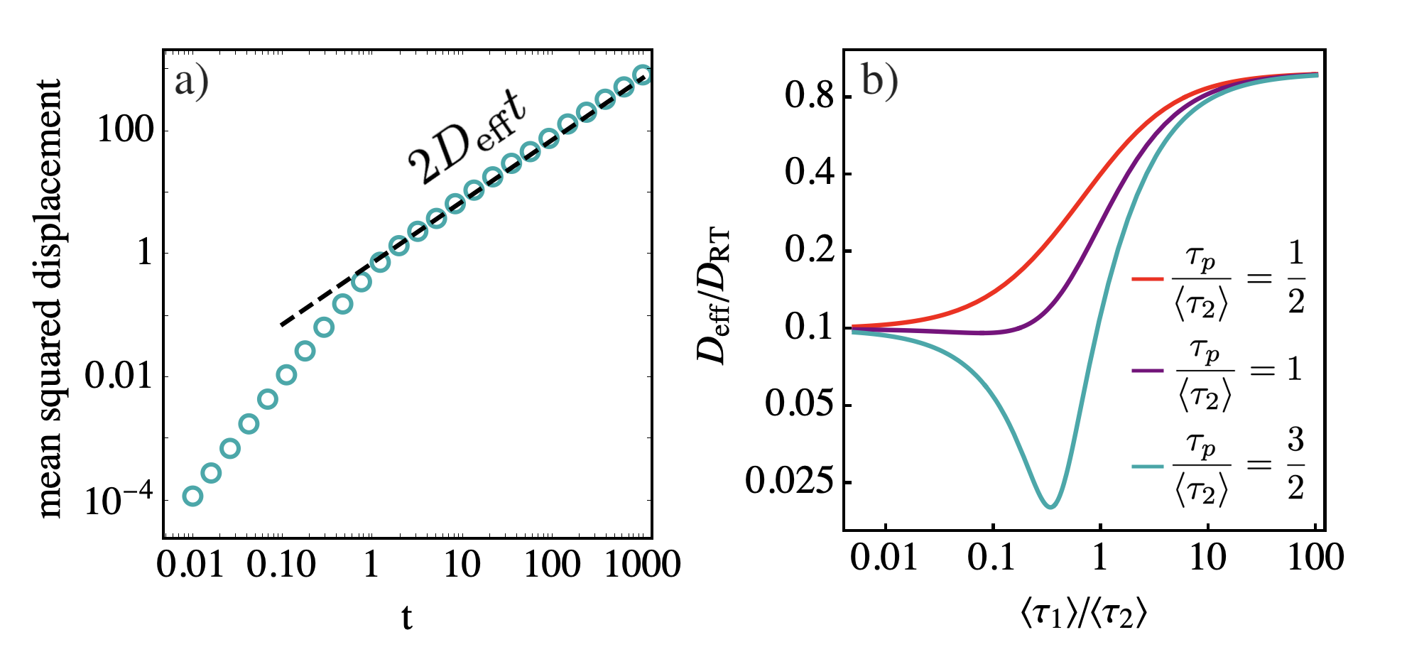
Fig.  2: a) Mean squared displacement of an active run-and-tumble particle intermittently switching to a passive phase. Active durations are drawn from a gamma distribution (32) with shape index $\gamma=3$. The dashed line shows theoretical prediction based on the effective diffusion coefficient [i.e., Eq. (3) with (33)], while circles show numerical simulation data. For simplicity, the passive phases have deterministic duration $\langle\tau_{2}\rangle=1/2$. Remaining parameters used are $v=1,\leavevmode\nobreak\ D=1,\leavevmode\nobreak\ \tau_{\rm p}=0.5$. b) Effective diffusivity rescaled with $D_{\text{RT}}\equiv v^{2}\tau_{\rm p}$ as a function of the ratio of active durations to passive durations, again for the case when active durations drawn from a gamma distribution (32) with shape index $\gamma=3$. In this case, we have set $D/D_{\text{RT}}=0.1$, so that passive phases are slow compared to the active motion.

In the case of intermittent active systems where the motion is interspersed with passive periods, we can use the above general formula (27) together with the known expression for the mean squared displacement of an active particle to obtain the effective diffusion coefficient. We let phase $1$ correspond to the active phase, and phase $2$ to the passive Brownian motion. Active particles are characterized by a persistence time $\tau_{\rm p}$, and the mean squared displacement takes the form ^{91, 92}

$$\langle x^{2}(t)\rangle_{1}=2v^{2}\tau_{\rm p}\left[t+\tau_{\rm p}\left(e^{-t/\tau_{\rm p}}-1\right)\right]\ ,$$ (28)

where $v$ is the self-propulsion speed. As the persistence time becomes smaller, a passive-like behaviour appears. Hence, active-passive switching can be thought of as the motion of an active particle that switched from persistent motion, to less persistent motion, for example as part of an intermittent search strategy.

The passive phase is diffusive with $\langle x^{2}(t)\rangle_{2}=2Dt$ where the passive diffusion coefficient is $D$. Eq. (27) then gives

$$D_{\text{eff}}= \frac{\langle\tau_{1}\rangle}{\langle\tau_{1}\rangle+\langle\tau_{2}\rangle}v^{2}\tau_{\rm p}+\frac{\langle\tau_{2}\rangle}{\langle\tau_{1}\rangle+\langle\tau_{2}\rangle}D$$

$$+\frac{v^{2}\tau_{\rm p}^{2}\left(\tilde{W}_{12}(\tau_{\rm p}^{-1})-1\right)}{\langle\tau_{1}\rangle+\langle\tau_{2}\rangle}\ .$$ (29)

This calculation remains general, and is valid for any waiting time density $W_{12}(t)$ in the active phase.

Therefore, a relevant question is how the choice of distribution of the active phase durations affect the effective diffusion coefficient. Since $\tilde{W}_{12}(\tau_{\rm p}^{-1})=\langle e^{-\tau/\tau_{\rm p}}\rangle$, we note that by Jensen’s inequality, we have $\tilde{W}_{12}(\tau_{\rm p}^{-1})\geq e^{-\langle\tau_{1}\rangle/\tau_{\rm p}}$. At fixed mean durations of the active phase, this inequality is saturated only by the deterministic case $W_{12}(\tau)=\delta(\tau-\langle\tau_{1}\rangle)$. Hence, at fixed durations of the two phases, the effective diffusivity is always smallest when the duration in the active phase is deterministic:

$$D_{\text{eff}}[W]\geq D_{\text{eff}}[\delta]\equiv D_{\text{eff}}^{\text{min}}\ .$$ (30)

Hence, fluctuations in the active phase durations are needed for effective spatial exploration.

Furthermore, since $\tilde{W}_{12}(s)\leq 1$ by monotonicity of integrals, we also have the upper bound

$$D_{\text{eff}}^{\text{max}}=\frac{\langle\tau_{1}\rangle}{\langle\tau_{1}\rangle+\langle\tau_{2}\rangle}v^{2}\tau_{\rm p}+\frac{\langle\tau_{2}\rangle}{\langle\tau_{1}\rangle+\langle\tau_{2}\rangle}D\ .$$ (31)

Hence, the effective diffusion coefficient is bounded as $D_{\text{eff}}^{\text{min}}\leq D_{\text{eff}}\leq D_{\text{eff}}^{\text{max}}$, with the explicit expressions given above (30) and (31).

To illustrate the above results, we specifically consider the case when the active durations are drawn from a gamma distribution:

$$W_{12}(\tau)=\frac{\tau^{\gamma-1}}{\tau_{0}^{\gamma}\leavevmode\nobreak\ \Gamma(\gamma)}e^{-\tau/\tau_{0}}\ ,$$ (32)

where $\Gamma(\cdot)$ is the Gamma-function. Its Laplace transform reads

$$\tilde{W}_{12}(\tau_{\rm p}^{-1})=\left(\frac{\tau_{\rm p}+\tau_{0}}{\tau_{\rm p}}\right)^{-\gamma}\ ,$$ (33)

From this, the effective diffusion coefficient can be easily obtained from Eq. (3). We note that in this case, the dependence on the duration of the passive Brownian phase enters only through its first moment, and is insensitive to further details of the distribution $W_{21}(\tau)$.

Figure 2a shows the mean squared displacement obtained numerically together with the theoretical prediction [i.e., Eq. (3) with (33)], verifying that the system’s long-time behaviour will be diffusive with the effective diffusion coefficient $D_{\rm eff}$ (27).

Figure 2b shows the effective diffusivity rescaled with the late-time pure run-and-tumble diffusion coefficient $D_{\text{RT}}\equiv v^{2}\tau_{\rm p}$, as a function of the ratio $\langle\tau_{1}\rangle/\langle\tau_{2}\rangle$.

4 Model: active particles with intermittent passive phases

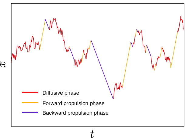
Fig.  3: Trajectory of a generalized run-and-tumble particle (orange and blue) with intermittent passive phases (red).

Section 2 discusses the framework of modelling processes switching between two arbitrary homogeneous dynamical phases. While general properties of such systems can be studied for symmetric processes, such as the effective diffusion coefficients in section 3, the framework is also capable of handling more involved processes with bias. In this section, we consider in detail the case of a (potentially biased) run and tumble particle (RTP) that intermittently switches to passive Brownian motion.

Let us consider the dynamics of an overdamped self-propelled particle in one dimension. Similar to the dynamics of the light-activated Janus particles ⁵⁷, this particle has three phases of motion: (i) A forward propulsion with a speed $v_{\rm f}$, when irradiated by a UV light; (ii) A backward propulsion with a speed $v_{\rm b}$ when irradiated by a green light; and (iii) A diffusive motion in the absence of light. Mathematically, the following equations model these phases:

$$\dot{x}(t)=\begin{cases}v_{\rm f}\quad&\text{forward propulsion},\\ -v_{\rm b}\quad&\text{backward propulsion},\\ \sqrt{2D_{\rm RS}}\eta(t)&\text{passive diffusion},\end{cases}$$ (34)

where $v_{\text{b,f}}\geq 0$, and $\eta(t)$ is a delta-correlated Gaussian white noise with zero mean: $\langle\eta(t)\eta(t^{\prime})\rangle=\delta(t-t^{\prime})$ and $D_{\rm RS}$ is the diffusion coefficient for the phase (iii).

We define the following switching mechanism between the three phases. The switching between the forward to backward propulsion and backward to forward propulsion (i.e., switching between UV and green light, and vice versa, respectively) happens at a rate $\alpha_{\text{fb}}$ and $\alpha_{\text{bf}}$, respectively. The switching from the active propulsion phase to the passive diffusive phase, (i.e., any light being turned off) occurs at a rate $\bar{r}_{\text{ap}}$; while the switching from the passive to the active phase, (i.e., any light being turned on) occurs at a rate $\bar{r}_{\text{pa}}$. Notice that we assume that when the lights are turned on, the particle can be either exposed to the UV or green light with equal probability. Furthermore, for simplicity, we consider a case where the particle always starts from the origin $x=0$ at time $t=0$ from any one of the active phases with equal probability.

It is always convenient to define a characteristic length- $\ell\equiv v_{\rm f}/\alpha_{\text{fb}}$ and a timescale $\mathcal{T}\equiv\ell/v_{\rm f}$. Then, Eq. (34) can be expressed in the dimensionless variables $x^{\prime}=x/\ell$ and $t^{\prime}=t/\mathcal{T}$. For convenience, we drop prime from these variables, and write

$$\dot{x}(t)=\begin{cases}1\quad&\text{forward propulsion},\\ -\theta\quad&\text{backward propulsion}\\ \sqrt{2D}\eta(t)&\text{passive diffusion}\end{cases}\ ,$$ (35)

where $\theta\equiv v_{\rm b}/v_{\rm f}$ measures the asymmetry in the backward to forward speed, and $D\equiv D_{\rm RS}\mathcal{T}/\ell^{2}$ is the dimensionless (rescaled) diffusion coefficient. The noise is again delta-correlated in time $\langle\eta(t_{1})\eta(t_{2})\rangle=\delta(t_{1}-t_{2})$. In the dimensionless units, the relative switching between backward to forward motion occurs at a rate $A=\alpha_{\rm bf}/\alpha_{\rm fb}$, and active-passive switching rates become $r_{\text{ap}}$ and $r_{\text{pa}}$.

In the following sections, we investigate this three-phase dynamics using the general switching formalism. To this end, we divide the dynamics Eq. (35) into (1) an active phase where the particle switches between a forward propulsion state and a backward propulsion state; and (2) a passive diffusive phase. The active phase, a generalized version of the one-dimensional RTP, is itself an example of a switching process, which we first analyze in the following subsection.

4.1 Generalized run-and-tumble particles in one dimension

Here, we discuss the scenario (1). The forward and backward propulsion are given by Eq. (35)(top two lines), they have the respective propagators,

$$P_{\rm f}(x,t) =\delta(x-t)\ ,$$ (36)

$$P_{\rm b}(x,t) =\delta(x-\theta t)\ ,$$ (37)

which in the Fourier-Laplace space read:

$$\tilde{\bar{P}}_{\rm f}(k,s) =\frac{1}{s-ik}\ ,$$ (38)

$$\tilde{\bar{P}}_{\rm b}(k,s) =\frac{1}{s+ik\theta}\ .$$ (39)

Suppose the particle begins in the forward phase. Using Eq. (19) for the exponential switching rate $A$ measuring relative rate with respect to forward-to-backward propulsion rate $\alpha_{\rm fb}$, we have for the Fourier-Laplace transform of the distribution $\tilde{\bar{p}}(k,s|f)$:

$$\tilde{\bar{p}}(k,s|f)=\dfrac{1+s+A+ik\theta}{s+ik\theta+(s-ik)(s+A+ik\theta)}\ .$$ (40)

Similarly, for the particle starting in the backward phase,

$$\tilde{\bar{p}}(k,s|b)=\dfrac{1+s+A-ik\theta}{s+ik\theta+(s-ik)(s+A+ik\theta)}\ .$$ (41)

We assume that the initial propulsion state of the active particle is chosen from the stationary state, $p(f)=A/(1+A)$ and $p(b)=1/(1+A)$. Using this, the Fourier-Laplace transform of the position distribution becomes

$$\tilde{\bar{p}}(k,s)= \tilde{\bar{p}}(k,s|f)p(f)+\tilde{\bar{p}}(k,s|b)p(b)$$ (42)

$$= \frac{k(1-A\theta)+i(1+A)^{2}+i\,s(1+A)}{(1+A)\left(s+ik\theta+(s-ik)(A+s+ik\theta)\right)}\ .$$ (43)

It is difficult to invert the above equation exactly to obtain a closed-form expression for the position distribution at all times. Nevertheless, $n$’th moment of the position fluctuations can be obtained by using Eq. (20). It turns out that the RTP is characterized by a non-zero mean,

$$\langle x(t)\rangle=\dfrac{A-\theta}{(1+A)}\leavevmode\nobreak\ t\ ,$$ (44)

as expected. Interestingly, the mean vanishes when $A=\theta$. We call this the ‘unbiased limit’ of the generalized RTP, where it has a zero mean in spite of having different velocities in the forward and backward propulsion phases. More precisely, the particle spends less time in the propulsion state with higher velocity, and more time in the lower velocity state, such that there is no net drift. This can be intuitively understood as follows. The system is initialized from the stationary probabilities of its forward and backward propulsion states, thus, at any time $t$, the average-time spent by the particle in the forward and backward phase, respectively, is $At/(1+A)$ and $t/(1+A)$, which amounts to the total displacements in the respective phase $At/(1+A)$ and $A\theta t/(1+A)$, respectively. The sum of these two displacements lead to (44). Interestingly, the mean vanishes for $A=\theta$. Notice that this is different from the ‘standard RTP’ limit (i.e., $A=\theta=1$), where again the mean is zero.

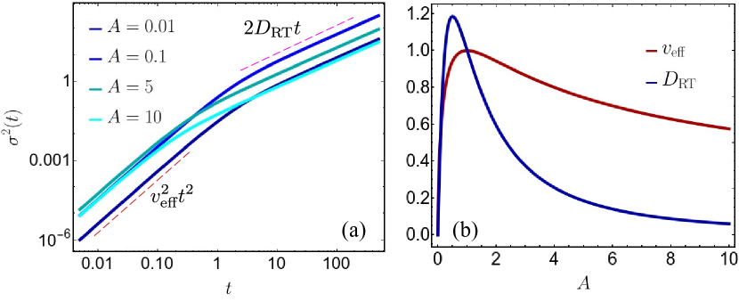
Fig.  4: Position fluctuations of a generalized RTP. Panel (a) shows the variance of the particle for different values of $A$, which crosses over from an initial ballistic phase to a late time diffusive phase at times $t\sim\min(1,A^{-1})$. Color intensity increases with increasing the value of relative switching rate between backward to forward motion, $A$. Panel (b) shows the variation of the effective velocity $v_{\rm eff}$ of the fluctuations and the effective diffusivity $D_{\rm eff}$ with respect to $A.$ For both plots $\theta=1.$

The variance $\sigma(t)^{2}\equiv\langle x^{2}(t)\rangle-\langle x(t)\rangle^{2}$ is obtained as,

$$\sigma^{2}(t)=\dfrac{2A(1+\theta)^{2}}{(1+A)^{4}}\left[e^{-(1+A)t}+t+At-1\right].$$ (45)

Therefore, similar to the usual RTP, the variance shows two dynamical regimes depending on the value of $\tau_{\text{RT}}\equiv\min(1,A^{-1})$,

$$\sigma^{2}(t)\approx\begin{cases}v_{\text{eff}}^{2}t^{2}&\qquad\text{ for }t\ll\tau_{\text{RT}},\\ 2D_{\text{RT}}t&\qquad\text{ for }t\gg\tau_{\text{RT}}\end{cases}\ .$$ (46)

where $v_{\text{eff}}$ and $D_{\text{RT}}$ denote the effective velocity of the fluctuations,

$$v_{\text{eff}}=\sqrt{2A}\frac{(1+\theta)}{(1+A)},$$ (47)

and the diffusion coefficient

$$D_{\text{RT}}=A\frac{(1+\theta)^{2}}{(1+A)^{3}},$$ (48)

respectively. Figure 4a discusses $\sigma^{2}(t)$ for different values of $A$ showing the ballistic and diffusive regimes of the variance. Figure 4b displays $v_{\text{eff}}$ and $D_{\text{RT}}$ as functions of $A$. Both are zero in the limits $A\to 0$ and $A\to\infty$, as in these limits, the particle is almost deterministic with very few tumbling events. However, at the intermediate values of $A$, $v_{\text{eff}}$ and $D_{\text{eff}}$ reach a maximum at $A=1$ and $A=1/2$, respectively. The magnitude of the relative propulsion speed $\theta$ does not influence the position of the maximum; however, it determines their respective maximum values.

We further compute the skewness, $\mathcal{S}(t)=\frac{\langle(x-\langle x\rangle)^{3}\rangle}{\sigma(t)^{3}}$, of the position distribution, which quantifies the asymmetry of a distribution with respect to its mean value. The skewness vanishes at long-time, with the leading order behaviour,

$$\mathcal{S}(t)\approx\frac{3(1-A)}{\sqrt{2(A+A^{2})}}\,t^{-1/2}.$$ (49)

The distribution becomes symmetric about its mean from a positively or negatively skewed distribution depending on $A>1$ or $A<1$. This is because for $A<1$, the time spent in the positive velocity phase is lesser compared to the time spent in the negative velocity phase.

Moreover, the excess kurtosis, $\mathcal{K}(t)=\frac{\langle(x-\langle x\rangle)^{4}\rangle}{\sigma(t)^{4}}-3$, can also be computed exactly and goes to zero as,

$$\mathcal{K}(t)\approx-\frac{6(1-4A+A^{2})}{A(1+A)t}.$$ (50)

The distribution thus tends to a Gaussian distribution from a platykurtic (negative kurtosis) or a leptokurtic side (positive kurtosis) for $2-\sqrt{3}<A<2+\sqrt{3}$, and $A\in(0,2-\sqrt{3})\cup(2+\sqrt{3},\infty)$, respectively. For very small or large $A$, the particle spends more time moving in one direction, thus the distribution approaches the corresponding normal distribution from one which is more sharply peaked, leading to the positive kurtosis. The negative kurtosis for intermediate values of $A$, on the other hand, occurs due to the competition of the time spent in the forward and backward motion, which are of the same order, causing more fluctuations resulting in the approach to the corresponding Gaussian distribution to happen from a flatter side.

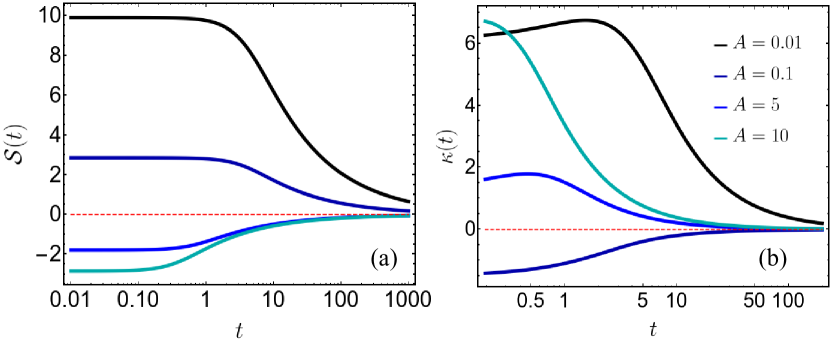
Fig.  5: Approach of the position fluctuations of generalized run and tumble particle to a Gaussian distribution. Skewness (a) and kurtosis (b) as a function of time $t$. Color intensity increases with increasing the value of $A$. We fix the speed asymmetry in backward to forward motion to $\theta=1$.

4.2 Run-and-tumble particles with intermediate passive phases

In the previous section 4.1, we discuss the case of an active particle in one dimension switching its directions (forward $\leftrightarrow$ backward), i.e., the generalized RTP. Herein, following the framework developed in Sec. 2, we extend our analysis to a case of a particle switching its motion between the generalized RTP and a passive (Brownian) dynamics. For convenience, we consider a case in which the particle is initialized in the generalized RTP phase (we refer to this phase as ‘phase 1’). The Fourier-Laplace transform of the propagator reads

$$\tilde{\bar{P}}_{1}(k,s)=\tilde{\bar{p}}(k,s)\ ,$$ (51)

where $\tilde{\bar{p}}(k,s)$ is given in (43). ‘Phase 2’, on the other hand, is a passive diffusion phase with its propagator in the Fourier-Laplace space:

$$\tilde{\bar{P}}_{2}(k,s)=\frac{1}{s+Dk^{2}}\ .$$ (52)

The general formula for the Fourier-Laplace transform of the position distribution (19) for waiting times being governed by Poisson distribution ($W_{ij}(t)\equiv r_{ij}e^{-r_{ij}t}$), is

$$\tilde{\bar{P}}(k,s)=\frac{\tilde{\bar{P}}_{1}(k,s+r_{\text{ap}})[1+r_{\text{ap}}\tilde{\bar{P}}_{2}(k,s+r_{\text{pa}})]}{1-r_{\text{ap}}r_{\text{pa}}\tilde{\bar{P}}_{1}(k,s+r_{\text{ap}})\tilde{\bar{P}}_{2}(k,s+r_{\text{pa}})}\ .$$ (53)

Thus, using the aforementioned $\tilde{\bar{P}}_{1}(k,s)$ (51) and $\tilde{\bar{P}}_{2}(k,s)$ (52) we find $\tilde{\bar{P}}(k,s)$ exactly [see Appendix A]. The expression of $\tilde{\bar{P}}(k,s)$ is rather long, and we relegate it to the Appendix A. Further, it is also difficult to invert this Fourier-Laplace transformed expression. Nonetheless, we compute the first four cumulants to understand the statistics of this switching process (i.e., generalized RTP $\leftrightarrow$ Brownian dynamics).

Employing (20) for Eq. (53), we compute the first position moment:

$$\langle x(t)\rangle=\frac{(A-\theta)}{(1+A)}\dfrac{r_{\text{ap}}[1-e^{-(r_{\text{ap}}+r_{\text{pa}})t}]+r_{\text{pa}}(r_{\text{ap}}+r_{\text{pa}})t}{(r_{\text{ap}}+r_{\text{pa}})^{2}}\ .$$ (54)

The mean position is independent of the diffusion coefficient, $D$, of the passive phase, since the only drift comes due to the particle’s active motion.

At short-time, the mean position retains exactly the same property as the generalized RTP (44):

$$\lim_{t\to 0}\langle x(t)\rangle=\frac{(A-\theta)}{(1+A)}t.$$ (55)

This can be understood as we consider that the particle always begins in the active phase, and in the short-time regime, $t\ll(r_{\text{ap}}$, there are typically no switching events. In the long-time regime, though there have been appreciable number of switching events, the mean is the same as Eq. (55), however, now weighed by the average time spent in the active phase:

$$\lim_{t\to\infty}\langle x(t)\rangle=\frac{r_{\text{pa}}}{r_{\text{ap}}+r_{\text{pa}}}\frac{(A-\theta)}{(1+A)}t\ .$$ (56)

The variance or the second cumulant captures the position fluctuations. In the following, we discuss its asymptotic behaviours [however, the full-time dependent form can be calculated using (20) for Eq. (53)]:

$$\sigma^{2}(t)\approx\begin{cases}\left[Dr_{\text{ap}}+\frac{A(v+1)^{2}}{(A+1)^{2}}\right]t^{2}\quad&t\ll\min\{1,A^{-1}\,r_{\text{ap}^{-1}}\}\\ \\ 2D_{\text{eff}}t\quad&t\gg\max\{1,A^{-1},r_{\text{ap}^{-1}}\},\end{cases}$$ (57)

where the effective diffusive coefficient is

$$D_{\text{eff}} =\frac{Dr_{\text{ap}}}{r_{\text{ap}}+r_{\text{pa}}}+\frac{r_{\text{pa}}(A+1)r_{\text{ap}}^{2}\left(A+\theta^{2}\right)+Ar_{\text{pa}}^{2}(\theta+1)^{2}}{(A+1)^{2}(A+r_{\text{ap}}+1)(r_{\text{ap}}+r_{\text{pa}})^{3}}$$

$$+\frac{r_{\text{pa}}r_{\text{ap}}\left[A^{3}+2Ar_{\text{pa}}(\theta+1)^{2}+\theta^{2}+A^{2}(1-2\theta)+A(\theta-2)\theta\right]}{(A+1)^{2}(A+r_{\text{ap}}+1)(r_{\text{ap}}+r_{\text{pa}})^{3}}\ .$$ (58)

Figure 6a displays the time evolution of the variance for different values of $r_{\text{ap}}$, indicating the short-time ballistic and long-time diffusive regime [see Eq. (57)].

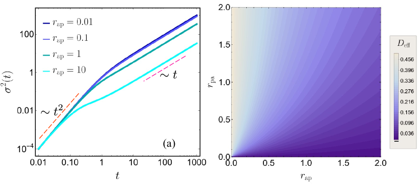
Fig.  6: Position fluctuation of a generalize run-and-tumble particle with intermediate passive phases. (a) Variance as a function of time $t$. The color intensity increases with active to passive switching rate $r_{\rm ap}$. We fix $r_{\text{pa}}=1$. The red and magenta dashed lines, respectively, indicate the short-time ballistic and long-time diffusive behaviour. (b) Effective diffusion coefficient in the $(r_{\text{ap}},r_{\text{pa}})$ plane. Here, we fix $A=1$ and $D=0.01$.

To investigate how the effective diffusion coefficient $D_{\rm eff}$ (4.2) changes with respect to the switching rates, we analyse $D_{\text{eff}}$ in the $(r_{\text{ap}},r_{\text{pa}})$ plane. To this end, we note that, in the limit $r_{\text{ap}}\to 0$, the effective diffusion coefficient $D_{\text{eff}}\to D_{\text{RT}}$. Moreover, since we consider the diffusion coefficient in the active phase $D_{\text{RT}}$ is larger than the diffusive phase (so that the diffusive phase is slower than the active phase), the effective diffusion coefficient of the particle is always peaked at the line $r_{\text{ap}}=0$. For finite values of $r_{\text{ap}}$, $D_{\text{eff}}$ increases with the increase in $r_{\text{pa}}$ as the time spent in the diffusive phases decreases. This is illustrated in Fig. 6b.

For the higher cumulants, we specifically focus on the case where $A=\theta$ (unbiased limit of the generalized RTP). It turns out that the skewness goes to zero in the long-time limit as

$$\mathcal{S}(t)=\frac{3r_{\text{pa}}(\theta-1)\theta\sqrt{r_{\text{ap}}+r_{\text{pa}}}}{\sqrt{2}\sqrt{r_{\text{ap}}+\theta+1}(Dr_{\text{ap}}(r_{\text{ap}}+\theta+1)+r_{\text{pa}}\theta)^{3/2}}t^{-1/2},$$ (59)

indicating the resulting distribution to be a symmetric one. Depending on the case, if $\theta$ is smaller or larger than unity, the distribution becomes symmetric from a positively or a negatively skewed distribution, respectively (Fig. 7a). Thus, though temporal-scaling remain unchanged compared to the generalized RTP model [c.f. (49)], the prefactor is modified.

The kurtosis can also be exactly computed and the leading order behaviour at long-time limit is given by,

$$\mathcal{K}(t) \approx t^{-1}\times\frac{6}{(r_{\text{ap}}+r_{\text{pa}})(r_{\text{ap}}+\theta+1)(Dr_{\text{ap}}(r_{\text{ap}}+\theta+1)+r_{\text{pa}}\theta)^{2}}$$ (60)

$$\Big{[}-D^{2}r_{\text{ap}}(r_{\text{ap}}-r_{\text{pa}})(r_{\text{ap}}+\theta+1)^{3}+Dr_{\text{ap}}\theta(r_{\text{ap}}+\theta+1)$$ (61)

$$\left(r_{\text{ap}}^{2}+r_{\text{ap}}(-5r_{\text{pa}}+\theta+1)-r_{\text{pa}}(2r_{\text{pa}}+3\theta+3)\right)$$ (62)

$$+r_{\text{pa}}\theta\big{(}r_{\text{ap}}^{2}\left(\theta^{2}+1\right)+2r_{\text{ap}}(r_{\text{pa}}(\theta-3)\theta+r_{\text{pa}}+\theta^{2}+\theta)$$ (63)

$$+r_{\text{pa}}^{2}((\theta-4)\theta+1)\big{)}\Big{]}\ .$$ (64)

The $t^{-1}$–coefficient’s sign determines if the kurtosis approaches Gaussian from a platykurtic or leptokurtic distribution. For very small or large $\theta$, the particle when in the active phase spends more time in moving in one of the run phases, leading to sharper distribution than the corresponding Gaussian distribution at long-time; leading to $\mathcal{K}(t)$ approach zero from the positive side. For intermediate $\theta$, on the other hand, the competition between the forward and backward runs are stronger, leading to stronger position fluctuations causing the distribution to approach Gaussianity from the negative side. This is shown in Fig. 7b for different values of $\theta$.

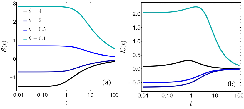
Fig.  7: Approach of the position fluctuations of generalized run and tumble particle to a Gaussian distribution with intermediate passive phases. Skewness (a) and kurtosis (b) as a function of time $t$. Here, we fix $r_{\text{pa}}=0.01$, $r_{\text{ap}}=1$, $D=0.01$ and different values of $\theta=A$.

5 Time evolution of the position distribution

In the previous section, we discussed the cumulants of the two different switching process. Here, we analyse the time-dependence of the density of a large number of non-interacting active particles with intermittent passive phase. For simplicity, we specialized to the case of the standard RTP (i.e., $A=\theta=1$) with $r_{\text{ap}}=r_{\text{pa}}=r$. The Fourier-Laplace transform of the probability distribution (53) in this case has a simpler form:

$$\tilde{\bar{P}}(k,s)=\frac{(r+s+2)\left(Dk^{2}+2r+s\right)}{Dk^{2}\left[k^{2}+(r+s)(r+s+2)\right]+k^{2}(r+s)+s(r+s+2)(2r+s)}.$$ (65)

Since the above (65) Fourier-Laplace transform is difficult to invert, we first discuss the time evolution behavior of the position distribution as seen from numerical simulations. Thereafter, we perform some asymptotic analysis.

Let us first discuss the time evolution of the position distribution qualitatively. From Fig. 8, we see that at short-time $t\ll\{1,r^{-1}\}$, the distribution has two different dynamical regions characterized by an RTP like behavior till $x=\pm t$, followed by non-trivial tail behavior, which we find asymptotically in Eq. (67); at $x=\pm t$, there are two Dirac-delta function-like peaks which can be attributed to the particles that have not changed propulsion states, or switched to passive state, in time $t$. With the increase in time, this peak vanishes, and the two dynamical regions combine, eventually becoming Gaussian-like at long-time, as also predicted from the cumulant analysis in the previous sections, see fig. 5. In the following, we also find the asymptotic distribution at very long-time, starting from Eq. (65).

5.1 Short-time distribution

A standard RTP is always bounded in the domain $[-t,t]$, which corresponds to it travelling ballistically without any tumbles. In this case, however, no such bounds exist and the fluctuations can go beyond $[-t,t]$ due to the intermittent passive phases. At times shorter than the typical switching time-scales, the leading order behaviour of the tails of the distribution can be predicted easily. In this regime $t\ll r^{-1}$, there are very few switches, and most of the contribution comes from the trajectories which have undergone one switching from an active to passive phase. The probability distribution beyond $x=\pm t$, can be written as,

$$P(x,t)\approx\sum_{j=\pm 1}\frac{1}{2}\int dx_{1}\int dt_{1}re^{-rt_{1}}\delta(x_{1}-jt_{1})e^{-r(t-t_{1})}\frac{e^{-\frac{(x-x_{1})^{2}}{4D(t-t_{1})}}}{\sqrt{4\pi D(t-t_{1})}}\ ,$$ (66)

where the particle switched to the diffusive phase at time $t_{1}$, with position $x_{1}$. Performing the delta function integral over $x_{1}$, we get,

$$P(x,t)\approx\sum_{j=\pm 1}\frac{1}{2}\int dt_{1}re^{-rt_{1}}e^{-r(t-t_{1})}\frac{e^{-\frac{(x-jt_{1})^{2}}{4D(t-t_{1})}}}{\sqrt{4\pi D(t-t_{1})}}\ .$$ (67)

An exact closed form of the above integral cannot be obtained. Nevertheless, the integration can be performed numerically and predicts the tail behaviour correctly in the short-time regime. This is compared with the tails of the position distribution at short-times, obtained from numerical simulations, which again shows a good agreement, see Fig. 8.

5.2 Long-time distribution

The behaviour of the distribution near the tails are dominated by contributions coming from small-$k$ behaviour. In this limit, the Fourier-Laplace transform simplifies Eq. (65) to,

$$\tilde{\bar{P}}(k,s)\approx\frac{(r+s+2)\left(2r+s\right)}{(r+s+2)\left[(r+s)\left(Dk^{2}+s\right)+s\right]+k^{2}(s+1)}\ .$$ (68)

Additionally, in the limit $s\to 0$, which corresponds to the long-time behaviour, the above equation (68) simplifies to:

$$\tilde{\bar{P}}(k,s)\approx\frac{1}{s+k^{2}[D+(2+r)^{-1}]/2}\ ,$$ (69)

which by inverting the Fourier and Laplace transform, leads to a diffusive Gaussian scaling of the tails at long-time:

$$P(x,t)=\dfrac{1}{\sqrt{2\pi t[D+(2+r)^{-1}]}}\exp\left(-\frac{x^{2}}{2t[D+(2+r)^{-1}]}\right).$$ (70)

This is compared to the distribution, obtained from numerical simulations at long-time, in Fig. 8, which shows a good agreement.

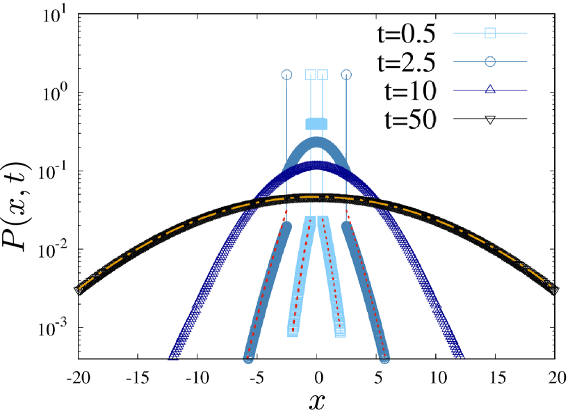
Fig.  8: Time evolution of the position distribution of the standard run-and-tumble particle with intermittent passive phases. Symbols: Numerical simulations. Dashed lines: analytical behavior of the tails (67) at short-times. Dot-dashed lines: Large-time Gaussian behavior (70). Here, we fix $D=1$ and $r=0.1$.

6 Summary

We analyzed a dynamical process characterized by a stochastic switching mechanism. By employing a trajectory-based approach, we derived the Fourier-Laplace transform of the position distribution for a particle undergoing such switching dynamics, with arbitrary waiting times. We calculated the generalized diffusion coefficient for this system, assuming the waiting time distributions possess a finite mean. We then applied this framework to an example of an active particle exhibiting intermittent diffusive phases, where we computed the exact expressions for the first few position cumulants. Additionally, we derived asymptotic expressions for the tails of the probability density function at all times, and our results were corroborated by numerical data.

Although our study focuses on one-dimensional processes, the general formulas we developed are applicable to any number of dimensions and can be utilized to investigate switching processes in higher-dimensional settings. The first-passage properties of these active processes display intriguing characteristics, particularly when compared to standard diffusion ⁹³. It would be interesting to explore whether intermittent diffusive phases could potentially enhance the first-passage times of active particles. Furthermore, another promising direction for future research is to examine the stationary distribution of such processes in the presence of a confining potential ⁹⁴ or under conditions of stochastic resetting ⁶³.

Appendix A Exact expressions used in the main text

In this section we provide the exact expressions for some of the expressions whose asymptotes or derivatives have been shown in the main text, namely skewness and kurtosis for the generalized RTP supplementing Sec. 4.1 and the generating function of the RTP with intermediate passive phases used in Sec. 4.2.

A.1 Generalized RTP

Using the generating function Eq. (43) and (20), the skewness of the position of the generalized RTP is given as,

$$\mathcal{S}(t)=-\frac{3(A-1)e^{-(A+1)t}\left(At+e^{(A+1)t}(At+t-2)+t+2\right)}{\sqrt{2}\sqrt{A}\left(At+e^{-(A+1)t}+t-1\right)^{3/2}}$$ (71)

which at large time, reduces to Eq. (49). Similarly, from the fourth moment of the position distribution, the kurtosis can be obtained as

$$\mathcal{K}(t) =\frac{1}{A\left(e^{(A+1)t}(At+t-1)+1\right)^{2}}\left(3e^{2(A+1)t}-3A\right.$$ (72)

$$\left.\times(-6A^{2}+2(A+1)((A-3)A+1)t+17A-6)+3e^{(A+1)t}\right.$$ (73)

$$\left.\left(A^{2}-1\right)^{2}t^{2}+4(A+1)((A-3)A+1)t+2A(3A-8)+6\right).$$

The above equation at long-times reduces to Eq. (50)

A.2 RTP with intermittent passive phases

The Fourier-Laplace transform of the distribution is given by,

$$\tilde{\bar{P}}(k,s) =\left(Dk^{2}+r_{\text{ap}}+r_{\text{pa}}+s\right)(k-A\theta k+i(A+1)(A+r_{\text{ap}}+s$$ (74)

$$+1))/\Bigg{[}(\alpha+1)z\left(H\left(Dk^{2}+r_{\text{pa}}+s\right)-r_{\text{ap}}r_{\text{pa}}(k-Ak\right.$$ (75)

$$\left.+i(\alpha+1)(A+r_{\text{ap}}+s+1))\right)\Bigg{]}.$$ (76)

Here,

$$H\equiv(A+1)(A(k+i(r_{\text{ap}}+s))+(k+i(r_{\text{ap}}+s+1))(ik\theta+r_{\text{ap}}+s)).$$ (77)