The Bénard–Conway invariant of two-component links
Abstract.
The Bénard–Conway invariant of links in the 3-sphere is a Casson–Lin type invariant defined by counting irreducible SU(2) representations of the link group with fixed meridional traces. For two-component links with linking number one, the invariant has been shown to equal a symmetrized multivariable link signature. We extend this result to all two-components links with non-zero linking number. A key ingredient in the proof is an explicit calculation of the Bénard–Conway invariant for –torus links with the help of the Chebyshev polynomials.
1991 Mathematics Subject Classification:
57K10, 57K311. Introduction
The practice of defining invariants of links in -manifolds using unitary representations of the link group has a long history. Xiao-Song Lin [11] defined an invariant of knots in by counting irreducible representations of the knot group sending the meridians to zero-trace matrices. Herald [8] and Heusener and Kroll [9] extended this construction by allowing matrices of a fixed trace which is not necessarily zero. The construction was further extended to links of more than one component by Harper and Saveliev [7] and Boden and Harper [2] by counting projective unitary representations. These invariants are closely related to gauge theory: for example, Floer homology theories of Daemi–Scaduto [6] and Kronheimer–Mrowka [10] can be viewed as categorifying the invariants of Lin and Harper–Saveliev, respectively.
The latest in this line of link invariants is the multivariable Casson–Lin type invariant of Bénard and Conway [1]. It is defined for colored links by counting irreducible representations of the link group sending the meridians to matrices of a fixed trace away from the roots of the multivariable Alexander polynomial. While this invariant is defined for links of any number of components, it is best studied for two-component links. In particular, for an oriented ordered link with linking number , Bénard and Conway [1, Theorem 1.1] identify with a symmetrized multivariable link signature of Cimasoni and Florens [5].
The purpose of this paper is to extend the result of Bénard and Conway to arbitrary oriented ordered links of two components with linking number . To be precise, we prove the following theorem.
Theorem 1.1.
thm:main-theorem-introduction Let be a two-component oriented ordered link with and, for any choice of , denote . If the multivariable Alexander polynomial of satisfies for all possible then
| (1) |
The proof of this theorem consists of two parts, just like the proof of [1, Theorem 1.1]. The first part shows that a crossing change within an individual component of changes both sides of the formula of \threfthm:main-theorem-introduction by the same amount. This fact was only proved in [1, Theorem 1.1] for links with , but that proof easily extends to links with , as we explain in Section 3. After changing enough crossings within individual components of , we only need to check that equation (1) holds for just one representative in each link homotopy class of . According to Milnor [12], link homotopy classes of two component links are completely characterized by , therefore, it is sufficient to prove \threfthm:main-theorem-introduction for –torus links with .
This second part of the proof occupies Sections 4, 5 and 6 of the paper. We compute the Bénard–Conway invariant directly from its definition and compare the answer with the symmetrized Cimasoni–Florens signature. The invariant , whose definition we recall in Section 2, is in an intersection number of two oriented curves in a -dimensional orbifold, traditionally referred to as a pillowcase. We come up with a parameterization of the pillowcase, in which the intersecting curves are given by explicit equations in terms of the Chebyshev polynomials; see Theorem 5.4. Checking the transversality and computing the intersection signs is then accomplished by a straightforward calculation.
Note that the above argument fails for links with because the base case, which is the link with , has a vanishing Alexander polynomial and hence its Bénard–Conway invariant is not defined.
The following result follows from Theorem LABEL:thm:main-theorem-introduction and the properties of the Cimasoni–Florens signature [5]. It is proved in Section 7 together with \threfthm:main-theorem-introduction.
Theorem 1.2.
thm:second-theorem-introduction For any two-component link as in the statement of Theorem LABEL:thm:main-theorem-introduction, the invariant is independent of the orientation of the link . Moreover, equals minus the Murasugi signature [15] of the link .
Acknowledgments: We thank Hans Boden, Anthony Conway, and Daniel Ruberman for useful discussions and sharing their expertise.
2. Preliminaries
In this section, we will recall the definitions of the Cimasoni–Florens signature [5] and the Bénard–Conway invariant [1] for oriented links in the 3-sphere.
2.1. The Cimasoni–Florens signature
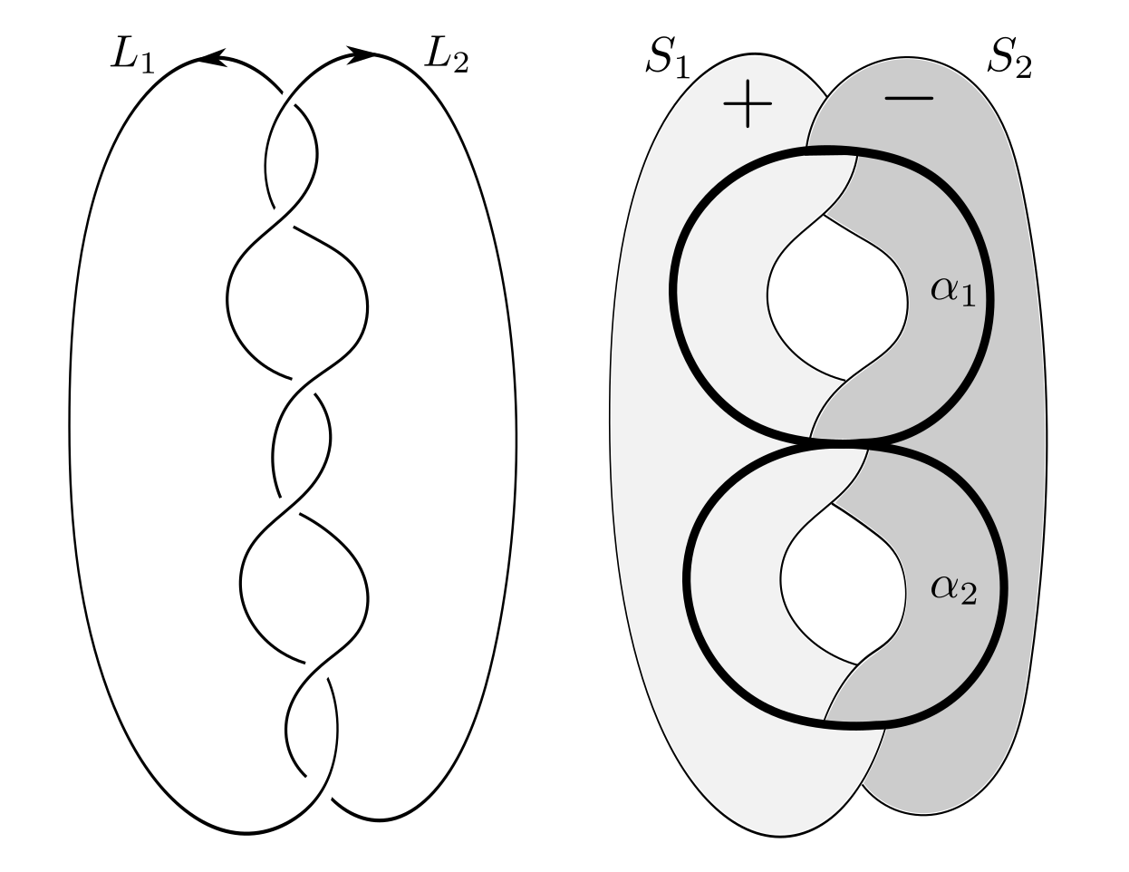
A –colored link is an oriented link whose components are partitioned into sublinks . A C-complex for a -colored link is a union of oriented surfaces in such that
-
(1)
for all , is a Seifert surface for (possibly disconnected, but with no closed components),
-
(2)
for all , is either empty or a union of clasps (see Figure 1), and
-
(3)
for all which are pairwise distinct, is empty.
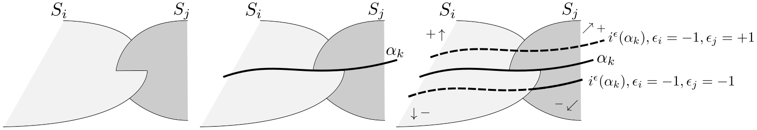
Such a C-complex exists for any colored link, see [4, Lemma 1] for the proof. A -cycle in a C-complex is called a loop if it is an oriented simple closed curve which behaves as illustrated in Figure 1 whenever it crosses a clasp. There exists a collection of loops whose homology classes form a basis of . Define by setting equal the class of the -cycle obtained by pushing in the –normal direction off for ; see Figure 1. Let
be the bilinear form given by where denotes the linking number. Fix a basis of and denote by the matrix of . If , then is the usual Seifert form and is the usual Seifert matrix. Also, note that for any .
Given a -colored link and a C-complex , fix a basis in and consider the associated Seifert matrices . Let be the matrix with coefficients in defined by
where summation runs over the possible sequences of ’s. For , set
| (2) |
Since , the matrix is Hermitian, hence its eigenvalues are real. Define the signature as the number of positive eigenvalues minus the number of negative eigenvalues. This signature does not depend on the choice of basis of , nor the choice of the C-complex of the link, thus it gives a well-defined isotopy invariant of the link ; see [5, Theorem 2.1] for the proof.
Definition 2.1.
Let be a -colored link and . The Cimasoni–Florens signature of is the function given by .
2.2. Colored links and colored braids
Before we go on to define the Bénard–Conway invariant of colored links, we will interpret the latter as the closures of colored braids; see Murakami [14].
Recall that the (Artin) braid group on strands is the finitely presented group with generators subject to the relations for each , and for . Geometrically, a generator can be viewed as the isotopy class of the braid whose -st strand crosses over the -th strand. The closure of a braid is the link obtained from by connecting the lower endpoints of the braid and its upper endpoints with parallel strands. The link is canonically oriented by choosing the downward orientations on the strands of .
A –colored braid is a braid together with an assignment to each of its strands of an integer (called the color) in via a surjective map. A –colored braid induces –colorings and on the upper and lower endpoints of the braid, which are –tuples of integers in . For any –coloring , the –colored braids with form a colored braid group . For example, if , then and is simply the braid group , and if and then is the pure braid group on strands.
The closure of a –colored braid , obtained from by connecting the lower endpoints of the braid with the upper endpoints with colored parallel strands, is a –colored link. A colored version of Alexander’s theorem states that every –colored link is the closure of a –colored braid , and a colored version of Markov’s theorem determines when two –colored braids have isotopic closures.
2.3. The Bénard–Conway invariant
Consider the Lie group of two–by–two unitary matrices with determinant one. We will be identifying it with the Lie group of unit quaternions via
| (3) |
and using the language of matrices and unit quaternions interchangeably.
Let be a free group on generators . The group acts naturally on via
| (4) |
This action induces an action on the representation space . More concretely, every braid induces a homeomorphism by the rule . For example, for the generator .
Let now be an oriented –colored link. Represent it as the closure of a –colored braid on strands. Given a –tuple , consider the representation space
Since the trace is preserved by conjugation, the homeomorphism constructed above restricts to a homeomorphism with the graph
Note that the trivial braid in gives rise to the graph which is just the diagonal
Since the product is preserved by the action of (see formula (4)), one immediately concludes that both and are subspaces of the ambient space
The group acts via conjugation on the spaces , and . We will restrict this action to irreducible representations, where it is free, and denote the quotient spaces by , and . These are smooth open manifolds of dimensions
see [1, Lemma 3.4].
The key observation now is that the points of the intersection are precisely the conjugacy classes of irreducible representations of the link group
| (5) |
sending the meridians to matrices of trace . From this point on, the definition of the Bénard–Conway invariant proceeds by making sense of the intersection number of and in . We will briefly outline the procedure and refer to [1] for detailed proofs.
Let be the multivariable Alexander polynomial of , and, given a –tuple , consider the finite set
| (6) |
Proposition 2.2.
prop:compactness If for all –tuples then the intersection is compact.
Let satisfy the condition of \threfprop:compactness. Since is compact, the graph can be perturbed if necessary using a perturbation with compact support to make the intersection transversal and hence a compact -dimensional manifold.
Next, we will orient all the manifolds in question. Denote by the conjugacy class of matrices in with the trace . Assuming that , the conjugacy classes are naturally homeomorphic to each other and to the standard 2-sphere . Choose an (arbitrary) orientation on . The space is a product of the spheres , , and we will endow it with the product orientation. The spaces and , which are diffeomorphic to via projection onto the first factors, will be endowed with the induced orientations. To orient , consider the map given by . Observe that , so that we can pull back the canonical orientation of to obtain an orientation on . Since the adjoint action of on each is orientation preserving, we can endow , , and with the induced quotient orientation.
The intersection number of and will be denoted by . The following proposition ensures that it only depends on the isotopy class of the closure of .
Proposition 2.3.
prop:markov-moves Under the assumptions of \threfprop:compactness, the intersection number is preserved by the Markov moves.
We will summarize the above construction in the following definition.
Definition 2.4.
def:invariant-def Let be a –colored link in and a –tuple. Let be a colored braid of strands whose closure is . Suppose that for all . Then the Bénard–Conway invariant of is well-defined by the formula
| (7) |
3. Inductive step for two-component links
From now on, we will restrict ourselves to 2-colored links of two components, which are just ordered two-component links. In this section, we will investigate what happens to the two sides of the formula (1) under a crossing change within a single component of .
Theorem 3.1.
thm:inductive-step Under the assumptions of \threfthm:main-theorem-introduction, the two sides of formula (1) stay well-defined and change by the same amount when a crossing change occurs within one of the components of the link.
The rest of this section will be dedicated to the proof of Theorem LABEL:thm:inductive-step. Given a pair , the set defined in (6) becomes
In addition, define the sets
and denote by the multivariable Conway potential function. Recall that equals up to multiplication by the powers of and .
Lemma 3.2.
lmm:inductive-lemma Let be a two-component oriented ordered link and denote by the link obtained from by a negative crossing change within a component of the link . Suppose that is such that, for all , one has , and . If and then
A proof of this lemma can be found in [1, Proposition 5.10 and Remark 5.11].
Lemma 3.3.
Let be an ordered two-component link with and suppose that is not a root of . Then
In addition, suppose that is obtained from by a negative crossing change within one of the components of , and that is not a root of either or . Then is either or .
A proof of this lemma can be found in [1, Lemma 6.2]. The following corollary is an easy consequence of the above lemma.
Corollary 3.4.
cor:inductive-cor Let be an ordered two-component link with and a link obtained from by a negative crossing change within one of its components. Suppose that is such that and . Then
We are now ready to sketch a proof of \threfthm:inductive-step, which will be a straightforward modification of the proof of Theorem 6.4 in [1]. That theorem is first proved under the additional assumption that and are transcendental. This assumption is then removed by showing that the invariant is locally constant in . Only the first part of the proof needs to be modified.
Observe first that a crossing change within one component of does not make the multivariable Alexander polynomial vanish, which ensures that the Bénard–Conway invariant of is well-defined. This follows from the Torres formula [16]
and our assumption that . Next, we will show that the two sides of the equation (1) change by the same amount under the crossing change. Assume without loss of generality that is obtained from by a negative crossing change in . According to \threflmm:inductive-lemma, we have
Note that has exactly two elements, and , where and . It now follows from \threfcor:inductive-cor that
which completes the proof.
4. representations of torus links
To complete the proof of Theorem \threfthm:main-theorem-introduction, it is sufficient to verify the formula (1) for –torus links with . Our convention here is that gives the right–handed torus link and the left–handed one. The verification will take up the rest of the paper. We begin in this section by describing the irreducible representations of the link group of with fixed meridional traces.
4.1. Geometry of
We will continue to identify matrices with unit quaternions as in (3). Any can then be written in the form , where and is a purely-imaginary unit quaternion. This expression is unique except when . We will refer to as the trace of and to as the real part of . Using arbitrary unit quaternions, can be conjugated to . Using only unit complex numbers, can be conjugated to for some . Alternatively, it can be expressed as for and with since the trace is conjugation invariant.
4.2. Counting the representations
Let us first assume that and consider the following presentation of the link group
where and are the meridians of the two components of . For a fixed choice of , we wish to describe the conjugacy classes of irreducible representations sending the meridians of the components of to matrices with the respective traces , .
Since , the relation is equivalent to commuting with . Therefore, we are looking for non-commuting unit quaternions and with prescribed traces such that commutes with .
Conjugate so that and for some . Since , the quaternions and commute only if the former is a complex number. In turn, this implies that because otherwise is a complex number and is reducible.
We end up looking for non-commuting unit quaternions and with prescribed traces such that is an –th root of (different from because otherwise is again reducible). The latter condition means that the real part of equals or, equivalently,
| (8) |
Proposition 4.1.
Given a –torus link with and a choice of , the number of the conjugacy classes of irreducible representations equals the number of integers such that
Proof.
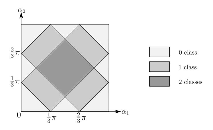
Example 4.2.
The cases of and correspond to the two oriented Hopf links. In both cases, the link group has no irreducible representations. The former case served as the base of induction in [1]. The count of conjugacy classes for is depicted in Figure 2. The diamond shapes in the figure have to do with the Alexander polynomial of the link as discussed in detail in the following subsection.
4.3. The Alexander polynomial
The number of the conjugacy classes of representations in Proposition 4.1 jumps with the change in and . The following proposition shows that these jumps occur at the roots of the multivariable Alexander polynomial, where the Bénard–Conway invariant is not defined.
Proposition 4.3.
prop:non-vanishing-condition Let be a –torus link with and its multivariable Alexander polynomial. Given , let . Then exactly when
| (9) |
Proof.
According to Milnor [13], the Alexander polynomial of is given by the formula
Therefore, exactly when is an –th root of unity that is not , which is equivalent to for some , up to addition or subtraction of . The result now follows. ∎
Remark 4.4.
When , the torus link is just the unlink of two components. Its multivariable Alexander polynomial is identically zero hence its Bénard–Conway invariant is not defined. This is the reason behind our assumption that .
5. The pillowcase and intersection theory
In this section, we will compute the Bénard–Conway invariants of –torus links as the intersection number of the manifolds and inside of . This will involve counting the representations described in Proposition 4.1 with plus/minus signs, after making sure that the intersection in question is transversal.
5.1. The setup
Let be a –torus link and assume that is positive. The case of negative can be treated in a similar manner, and both cases will be discussed in detail when we perform explicit calculations in Section 5.5. Let be such that and for any and . This condition guarantees that the Bénard–Conway invariant of is well-defined; see Proposition LABEL:prop:non-vanishing-condition. We will view the link as a -colored link which is the closure of the –colored braid with the –coloring . The Bénard–Conway invariant of is then the intersection number of and inside of . Our first goal will be to parameterize these manifolds.
5.2. The pillowcase
Recall that is an open 2-manifold obtained by removing the conjugacy classes of reducible representations from the orbifold , where
In the special case of , the orbifold is referred to as a pillowcase; see for instance Lin [11]. We will extend this terminology to the general case.
After conjugation, we may assume that and , where with ; see Section 4.2. Write and , where and are purely imaginary unit quaternions. For any given , the equation can be uniquely solved for if and only if the trace of matches that of , that is,
Write , where , then the above equation is equivalent to
| (10) | ||||
We will handle the case of first. In this case, equation (10) has the form , where and
is a non-zero vector (because its third coordinate is never zero). Therefore, equation (10) describes a plane in the space of purely imaginary quaternions, and our task becomes describing the intersection of this plane with the unit sphere of purely imaginary unit quaternions given by the equation . Note that the point on the plane closest to the origin is given by . One can easily see that the distance from this point to the origin equals
| (11) |
and that this distance is strictly less than one, making the intersection of the plane with the unit sphere a circle for any choice of . Therefore, away from the points with and , the orbifold is homeomorphic to a cylinder . It can be parameterized as follows.
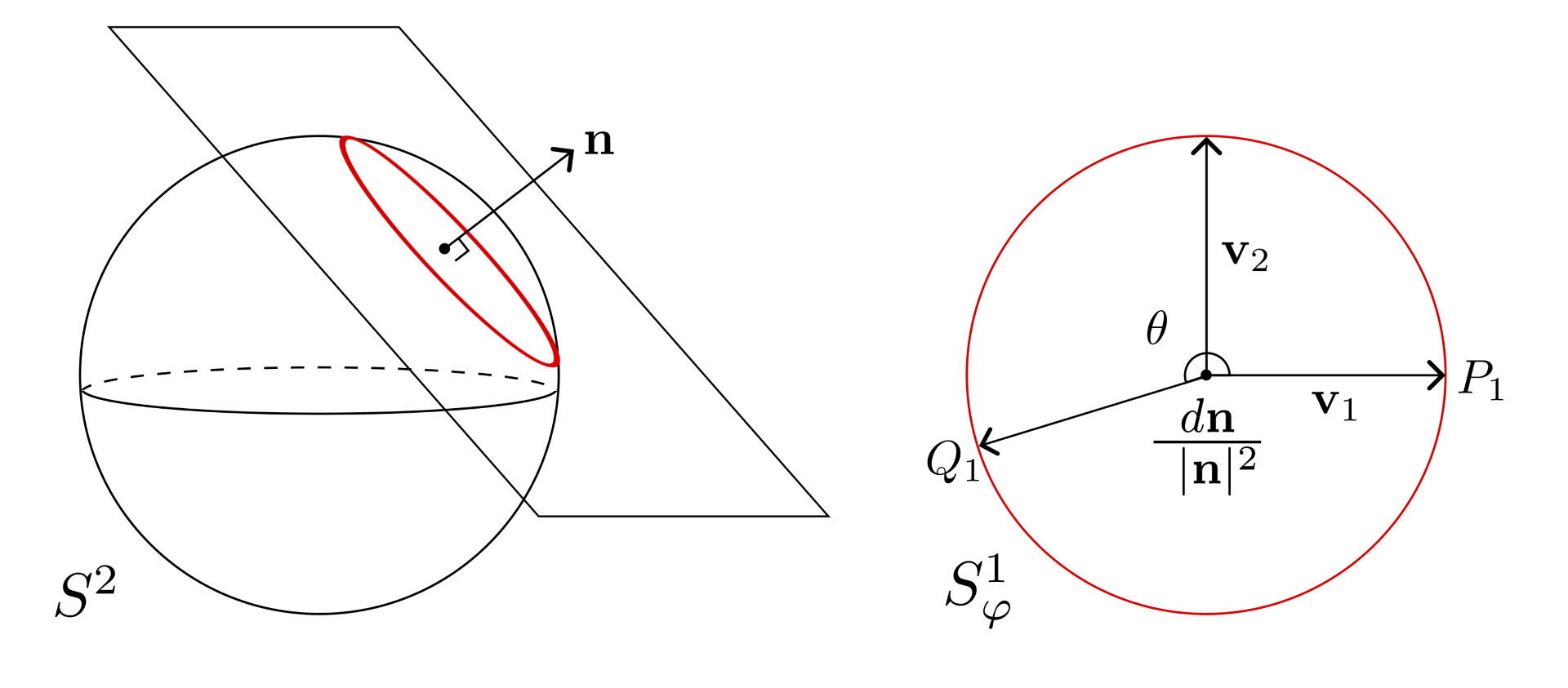
Note that the circle contains the vector , which corresponds to the solution with of the equation (10) . Let
Since the vectors and are orthogonal to each other, we can write
| (12) |
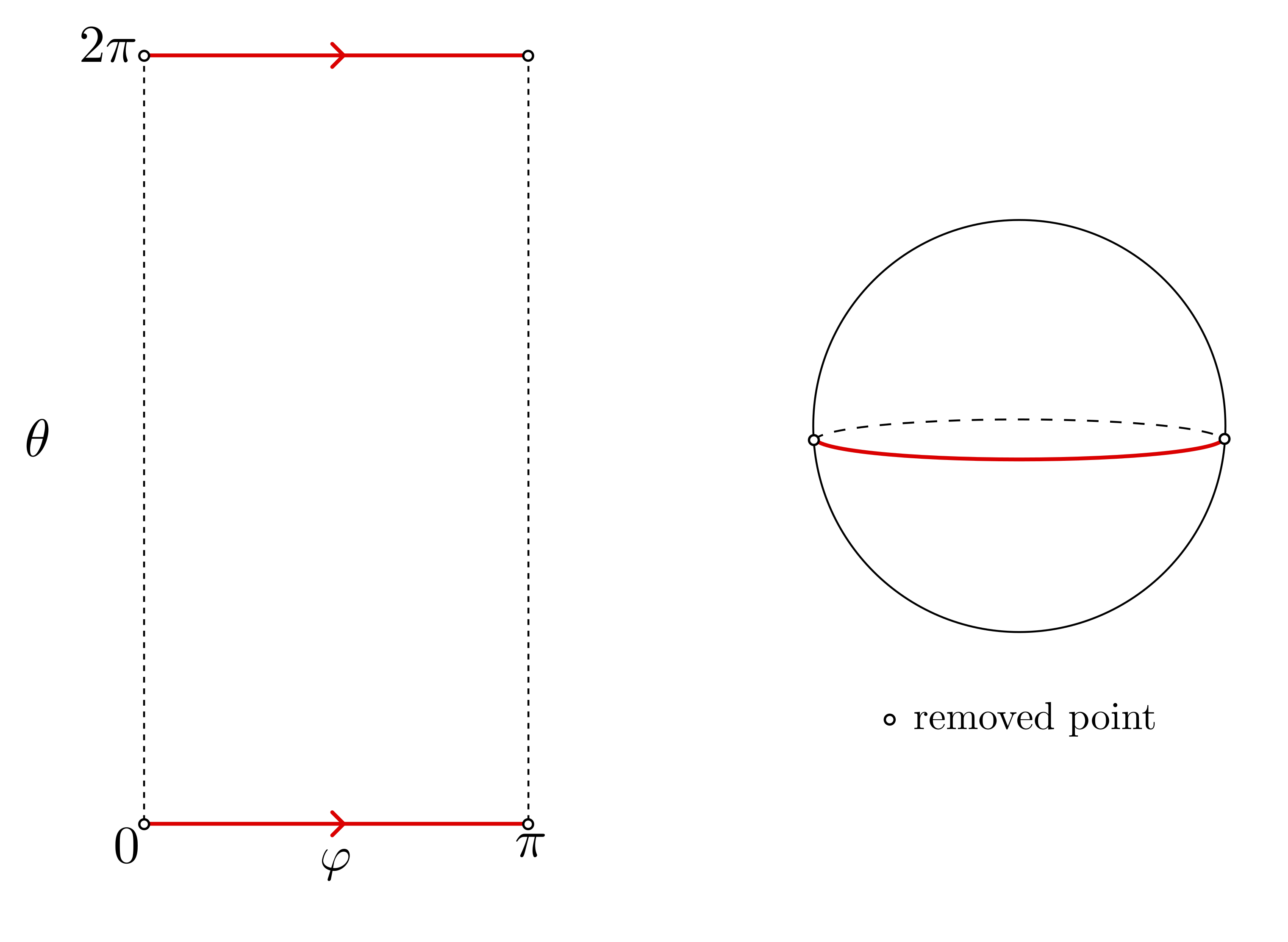
for some ; see Figure 3. Therefore, away from the points with and , the cylinder is parameterized by with the intervals and identified; see Figure 4.
We now turn to the full space . It is a compactification of the cylinder described above by the points with and . The type of compactification one obtains depends on and
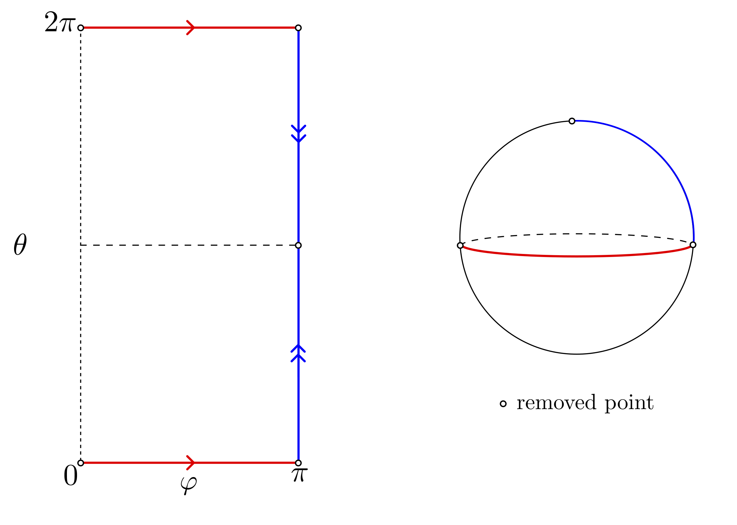
(1) For a generic choice of and with , the above calculation extends to the points with and giving rise in each case to a single reducible representation. In this case, the cylinder compactifies to a 2-sphere, and is a 2-sphere with two points removed; see Figure 4.
(2) The case of , in which but , was investigated in [9]. In this case, all representations with and are irreducible and the points and are identified; see Figure 5. Topologically, is a 2-sphere with three points removed.
(3) In the special case of and we have but . This time around, the representations with and are irreducible and is a mirror image of Figure 5.
(4) The remaining case of is the original case investigated by Lin [11]. The representation with and are now irreducible for all . The resulting is a sphere with four points removed.
All of the resulting orbifolds will be referred to as pillowcases. The calculation that follows will be the same for all of them because it happens away from the points with and .
5.3. Intersection theory in the pillowcase
The diagonal is a subspace of given by the equation . In our parameterization of the pillowcase, is then exactly the subspace where or . It is shown in red in Figure 4.
Next, we will parametrize . Since is the angle between the vectors and , we have
Using formula (11), this simplifies to
| (13) |
The lemmas that follow simplify this formula further and eventually lead to Theorem 5.4, which identifies the right hand side of (13) as a Chebyshev polynomial.
Lemma 5.1.
The right hand side of formula (13) is a polynomial in , which will be denoted by .
Proof.
We will proceed by simplifying (13) while keeping track of its dependence on . By a direct calculation,
| (14) |
where , and are real valued polynomials in of degrees , and . To compute , recall that is the image of under the action of the braid , where ; see Section 2.3. Therefore,
and
Write
where and are complex valued polynomials in of degrees and . Using an induction on one can easily see that
where and are complex valued polynomials in of degrees and . A straightforward calculation then shows that
| (15) |
where , and are real valued polynomials in of degrees , and . By taking the dot product of (14) and (15) we conclude that the numerator of (13) has the form times a polynomial in of degree at most . The factors of in the numerator and the denominator of (13) cancel, thereby finishing the proof. ∎
Lemma 5.2.
The polynomial has degree and its leading coefficient equals .
Proof.
We will follow the proof of the previous lemma but make our calculations more precise. One can check using induction on that
| (16) |
where the dots stand for a polynomial in of degree at most . A tedious but direct calculation of the polynomials in formulas (14) and (15) then yields the following formulas :
and
The brackets in the formulas for , and contain polynomials whose degrees are indicated by the subscripts. Note that the first bracket in the formula for has degree rather than , which follows from (16). Another lengthy calculation shows that
where the dots stand for a polynomial in of degree at most . Using formula (16), this further simplifies to
which is a polynomial of degree . It follows that is a polynomial of degree whose leading term matches that of the polynomial . Another induction shows that the leading term of equals
which completes the proof. ∎
Lemma 5.3.
The polynomial evaluates to, respectively, and at and .
Proof.
We will use formula (13), which defines for , to show that limits to, respectively, and as and . We first calculate the limit as . Once we eliminate the factors as in Lemma 5.1, the calculation reduces to evaluating the expression
at . Here, we use the notation from the proof of Lemma 5.2. It is easy to see that , , evaluate to
To evaluate and , we will keep track of in the formula while setting equal to one. An induction on can be used to show that
| (17) |
where and the dots stand for higher degree polynomials in . Using the identity
the above formulas can be written in trigonometric form. It now follows from the formula
that, when , we have
Finally, a tedious but straightforward trigonometric calculation using the above formulas shows that
which immediately implies that limits to as . The calculation of the limit as is similar. ∎
Recall that the Chebyshev polynomial of the first kind is the unique polynomial of degree satisfying the formula for The following theorem is the main result of this section.
Theorem 5.4.
Let be the Chebyshev polynomial of the first kind of degree . Then the formula (13) is equivalent to
| (18) |
Proof.
The solutions of the equation with are precisely the intersection points of and in the pillowcase . According to (5), these correspond to the conjugacy classes of irreducible representations , which we described as the values of solving equation (8). Note that the function achieves its absolute maximum at all such hence we also know that .
Let us first assume that the values of are in a sufficiently small neighborhood of chosen so that equation (8) has the maximal possible number of solutions, which is . Consider the polynomial
This polynomial has roots , , each of multiplicity at least two. In addition, it has roots by Lemma 5.3. On the other hand, the degree of is at most by Lemma 5.2, while the leading coefficients of and match by Lemma 5.2. Therefore, the degree of is at most so must vanish.
To finish the proof, we observe that both polynomials and are analytic functions in . Since we proved that they equal each other in an open neighborhood of , they must equal each other for all . ∎
5.4. Transversality
In general, need to be perturbed for the intersection number (7) to make sense. However, in the case of –torus links, no perturbation is necessary as the intersection is automatically transversal.
Proposition 5.5.
Let be the braid whose closure is the –torus link with . Then the intersection of and in is transversal, and all the intersections points contribute with the same sign into the algebraic count.
Proof.
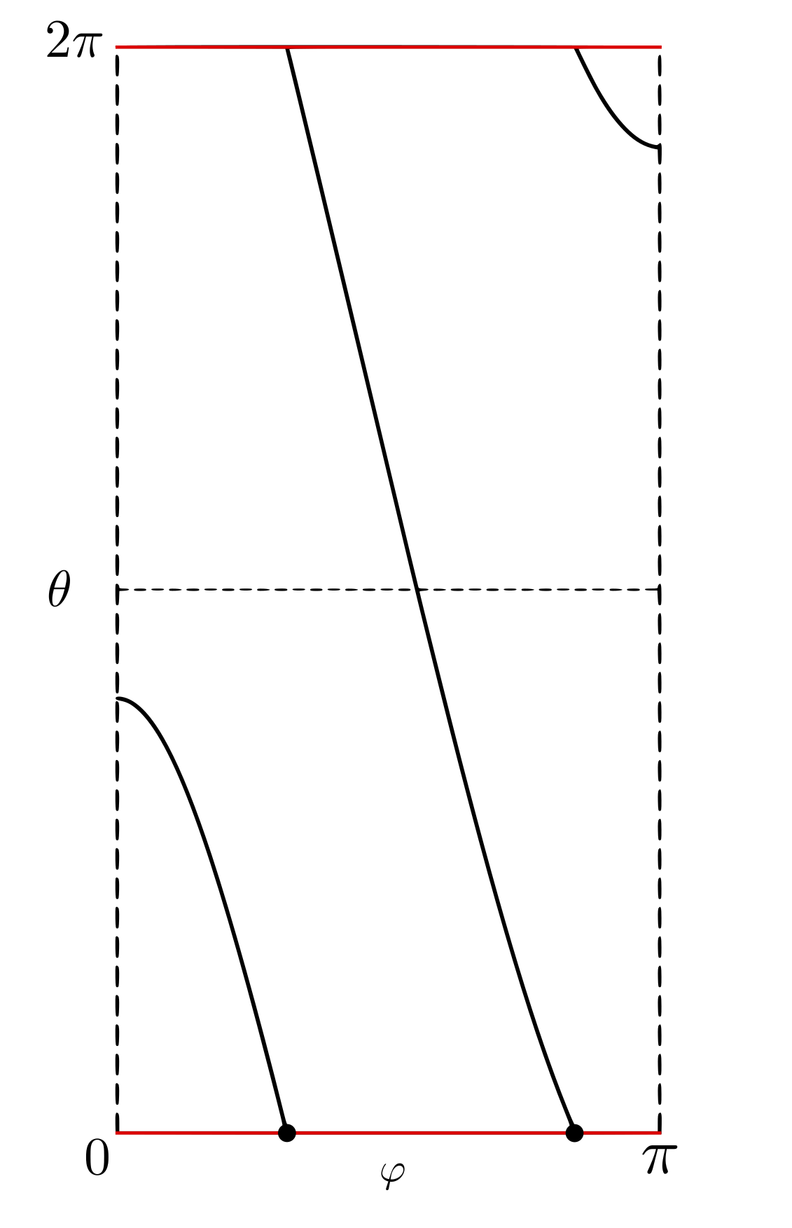
We wil assume that since the case of can be handled similarly. The curves and intersect exactly at the points , where solves the equation
which we have shown happens exactly when
The curve is smooth near each of the intersection points. It is parameterized by , where is a smooth function of found by solving the equation (12). The intersection points give local maxima of the Chebyshev polynomial hence the curve must be decreasing near these points as shown in Figure 6. Therefore, all the intersection numbers will be of the same sign once we prove that the intersections are transversal.
To prove transversality, it suffices to show that the derivative of with respect to is not zero near the intersection points. Differentiating the formula (18) and keeping in mind that , where is the Chebyshev polynomial of the second kind of degree , we obtain
We wish to show that, as from the left, the limit of the right hand side of this equation is non-zero. This is true because of the well known fact that each is a simple root of and a double root of . ∎
5.5. Fixing the overall sign
An immediate corollary of Proposition 4.1 and Proposition 5.5 is that, up to an overall sign, the Bénard–Conway invariant of the –torus link equals the number of integers such that
To determine the sign, we need to get specific about the orientations of , and and to compute at least one intersection number explicitly. We will only compute the intersection number in the special case of . The calculation for general and will be similar, and the case of negative will be addressed later in this section. The following argument is a modification of the argument of Boden and Herald [3].
In the case at hand, intersects at one point , which corresponds to the conjugacy class of in . Consider the function given by and the function given by
The latter is exactly the quadruple used to parameterize the pillowcase , with substituted in the equation. Notice that is the quotient of by conjugation. We will orient and by applying the base–fiber rule.
First, we will consider the map . Two tangent vectors that span the tangent space to at are given by
The tangent space to the orbit through is spanned by the vectors
The vectors form a basis of . Complete it to a basis for using the vectors , where we can choose , , and . Notice that the orientation of the ordered triple is consistent with that of the standard basis of Lie algebra .
The oriented bases and of are related by the matrix
of determinant is . This implies that the ordered pair gives a positively oriented basis in .
Next, consider the one–variable parameterizations and , where is the homeomorphism induced by the braid. Compute the tangent vector
to and the tangent vector
to . The bases and in the tangent space are related by the matrix
Since the determinant of this matrix is positive, we conclude that the intersection number equals .
Corollary 5.6.
For any integer and for any choice of away from the set (9), the Bénard–Conway invariant of the –torus link is well defined and is equal to the number of integers such that
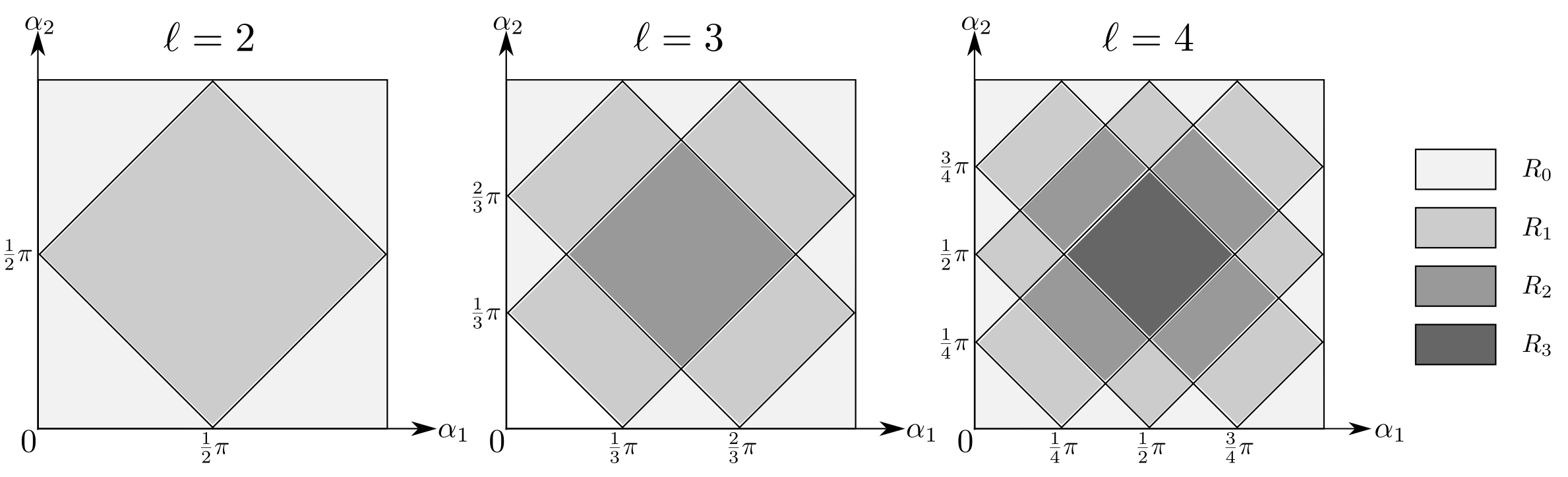
For , we obviously obtain , as established by Bénard and Conway [1]. For the first few , the invariant equals in each of the respective diamond–shaped regions depicted in Figure 7. The boundaries of consist of the values of from the set (9), where the multivariable Alexander polynomial of vanishes and hence the Bénard–Conway invariant is not defined.
We will finish this section by computing the invariant with . The link is the closure of the braid and the above calculation for and can be repeated word for word. The only essential change occurs in parameterizing , which produces the tangent vector
The basis is now related to the basis by the matrix
of negative determinant. This brings us to the following conclusion.
Corollary 5.7.
For any integer and for any choice of away from the set (9) the invariants and are well defined and related by the formula
6. Multivariable signature for torus links
The goal of this section is to calculate the Cimasoni–Florens signature of the –torus link , together with the quantity , and to finish the proof of \threfthm:main-theorem-introduction.
6.1. The positive linking number
We will start by computing the Cimasoni–Florens signature of the 2-colored link with . The signature in question is the signature of the matrix , where
as in formula (2). Using the C-complex shown in Figure 8, we can easily see that and are always zero matrices; is the matrix with on the main-diagonal and on the super-diagonal, and . In particular, the matrices are empty in the case of . Thus, is the matrix with on the main-diagonal, on the super-diagonal, and on the sub-diagonal.
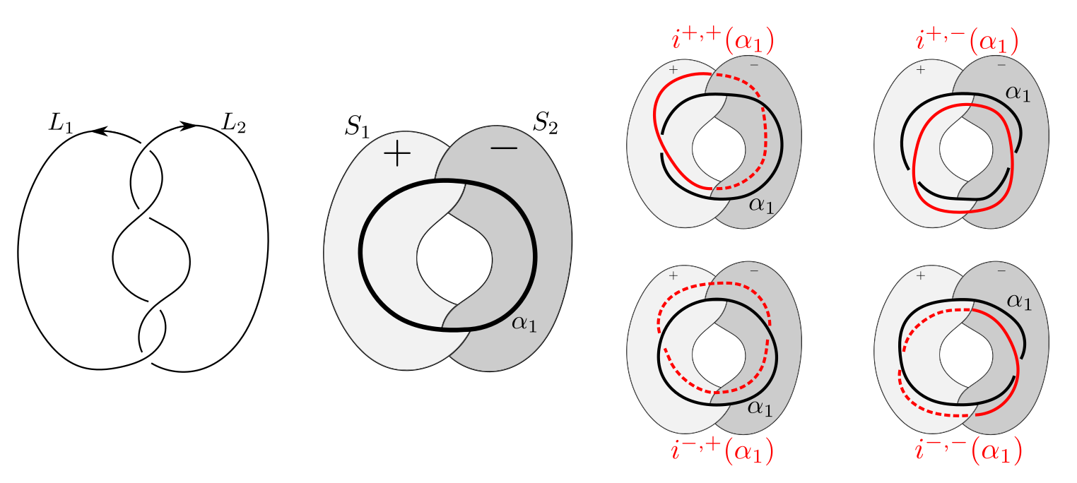
Example 6.1.
A C-complex for the –torus link and the curves are shown in Figure 8. The complex is homotopy equivalent to a circle, with generated by . Thus, for each , the associated Seifert matrix is the matrix . A direct counting gives that , , and thus is the matrix . In particular, or depending on the sign of the real number .
Example 6.2.
A C-complex of the -torus link is shown in Figure 9. The complex is homotopy equivalent to the one–point union , with and forming a basis of . By direct calculation,
Therefore,
Notice that the top-left -minor of is precisely .
We will now move on to the general case. For any let so that , the determinant of empty matrix, etc. In general, we have a recursive relation
Since , we can write with and re-write the above formulas in trigonometric form so that , , plus the recursive relation
This recursive relation has a unique solution
| (19) |
where is the –th Chebyshev polynomial of the second kind, . A direct calculation now shows that the signs of are given by the formula
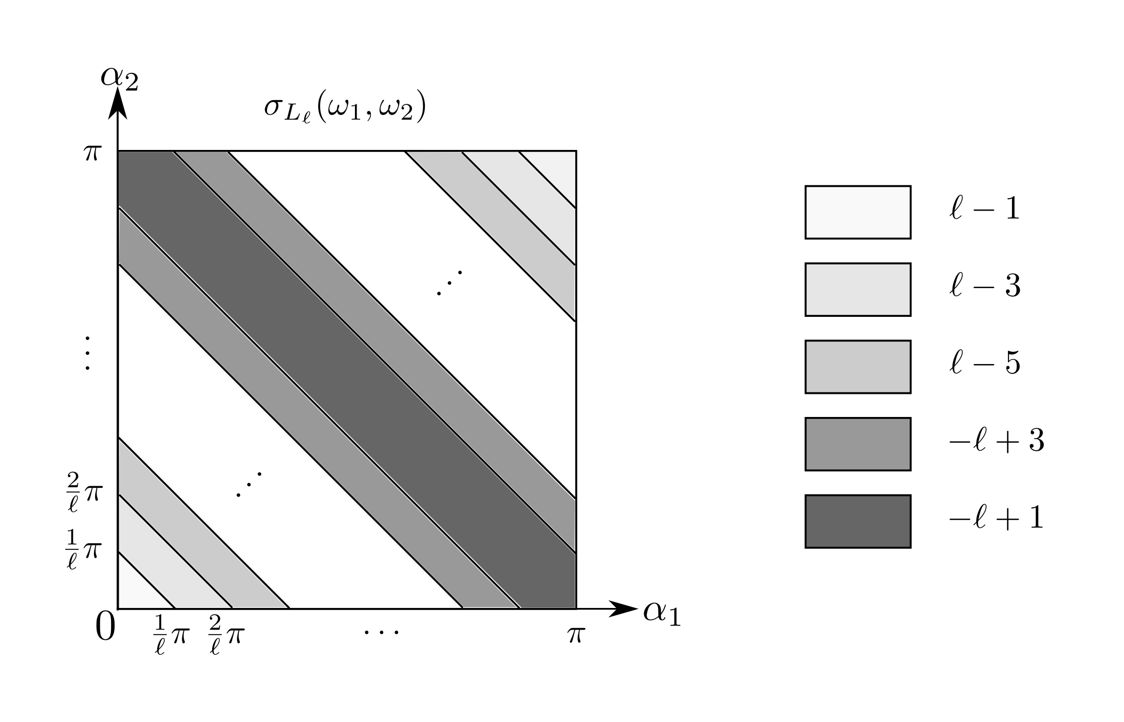
Since the top-left minor of for is precisely , we can use the Sylvester criterion to compute the signature by the formula
which is equivalent to the formula
see Figure 10 for a graphic depiction.
6.2. The negative linking number
For any positive integer and , we calculate , , and we obtain the recursive relation
which has the unique solution
which is obtained by a shift by of the formula (19). In the application of the Sylvester criterion, each of the summands flips the sign compared to the positive linking number case, that is, and for each from to . Thus we obtain
Recall that , see Corollary 5.7. Therefore, the formula (20) at the end of the last subsection extends to the following result.
Theorem 6.3.
thm:base-step Let be the –torus link with and, for any choice of , let . If the multivariable Alexander polynomial of satisfies for all possible , then
7. Proof of Theorems LABEL:thm:main-theorem-introduction and LABEL:thm:second-theorem-introduction
According to [12], the linking number is a complete invariant of link homotopy for two-component links. Therefore, any two-component oriented link with linking number can be obtained from the –torus link via a sequence of crossing changes within individual components. According to \threfthm:base-step, the equality (1) holds for all –torus links with , and according to \threfthm:inductive-step, the equality (1) remains true with each crossing change. Theorem LABEL:thm:main-theorem-introduction now follows.
In order to prove Theorem LABEL:thm:second-theorem-introduction, we will use the following formula of Cimasoni and Florens [5, Proposition 2.8],
where stands for the component with reversed orientation. Together with the formula
which easily follows from the definition of the Cimasoni–Florens signature, it implies that
is independent of the choice of orientation on the link . If , one can use the following formula of [5, Proposition 2.5],
relating the multivariable signature with the Levine–Tristram signature , to obtain
In the special case of , this implies that equals minus the Murasugi signature of .
Remark 7.1.
There does not appear to exist a name in the literature for the quantity nor for a similar quantity for links with more than two components when . Perhaps it should be called the equivariant Murasugi signature.
References
- [1] L. Bénard, A. Conway, A multivariable Casson–Lin type invariant, Ann. Inst. Fourier (Grenoble) 70 (2020), 1029–1084
- [2] H. Boden, E. Harper, The SU(N) Casson–Lin invariants for links, Pacific J. Math. 285 (2016), 257–282
- [3] H. Boden, C. Herald, The SU(2) Casson-Lin invariant of the Hopf link, Pacific J. Math. 285 (2016), 283–288
- [4] D. Cimasoni, A geometric construction of the Conway potential function, Comment. Math. Helv. 79 (2004), 124–146
- [5] D. Cimasoni, V. Florens, Generalzied Seifert surfaces and signatures of colored links, Trans. Amer. Math. Soc. 360 (2008), 1223–1264
- [6] A. Daemi, C. Scaduto, Equivariant aspects of singular instanton Floer homology, Geometry Topol. (to appear) arXiv:1912.08982
- [7] E. Harper, N. Saveliev, A Casson–Lin type invariant for links, Pacific J. Math. 248 (2010), 139–154
- [8] C. Herald, Flat connections, the Alexander invariant, and Casson’s invariant, Comm. Anal. Geom. 5 (1997), 93–120
- [9] M. Heusener, J. Kroll, Deforming abelian -representations of knot groups, Comment. Math. Helv. 73 (1998), 480–498
- [10] P. Kronheimer, T. Mrowka, Khovanov homology is an unknot-detector, Publ. Math. Inst. Hautes Études Sci. 113 (2011), 97–208
- [11] X.–S. Lin, A knot invariant via representations spaces, J. Differential Geom. 35 (1992), 337–357
- [12] J. Milnor, Link groups, Ann. of Math. 59 (1954), 177–195
- [13] J. Milnor, Singular Points of Complex Hypersurfaces. Princeton University Press, 1968
- [14] J. Murakami, A state model for the multivariable Alexander polynomial, Pacific J. Math. 157 (1993), 109–135
- [15] K. Murasugi, On the signature of links, Topology 9 (1970), 283–298
- [16] G. Torres, On the Alexander polynomial, Ann. of Math. 57 (1953), 57–89